Compound and Consecutive Extreme Events in Salzburg Under Different Climate Change Scenarios: Combining Stakeholder Insights with Future Climate Model Projections

Abstract

Compound and consecutive extreme events are increasingly understood as key contributors to climate risk, as their interactions can intensify impacts beyond those produced by individual hazards alone threatening the long-term sustainability of regional infrastructure. Compound coincident events involve multiple climate drivers or hazards that occur simultaneously or in close temporal proximity, exhibiting overlapping spatial and temporal characteristics. For assessing multi-hazards, information on critical thresholds of the events investigated (extreme precipitation and wind gusts in the presented study) is key, as is the time frame needed to determine the probability of event B after an event A. As this data is location-specific, stakeholder integration provides a potential tool for gathering this information to enable socially robust disaster risk management. The presented study displays a potential interdisciplinary approach to how multi-hazards and their occurrence can be investigated locally. Therefore, stakeholder integration is combined with climate model output and a copula-based analysis of compound coincident and consecutive extreme daily wind and precipitation events for the Salzburg region under different climate change scenarios (SSP1-2.6, SSP5-8.5). Through stakeholder integration, relevant thresholds and potential time frames were identified. Our findings indicate that the thresholds critical to the considered assets (properties, transport, energy) are well aligned between different stakeholders; however, the time frame of increased vulnerability due to a previous event differs strongly between them. Compared to the baseline scenarios, the ranges within the climate model used for rainfall and wind speed intensity under SSP1-2.6 and SSP5-8.5 scenarios are examined, and, for rainfall, have expanded to greater values for both compound coincident and consecutive events, highlighting challenges and future research needs for sustainable adaptation and regional policy.

1. Introduction

Compound coincident and consecutive extreme events are increasingly recognized as critical drivers of climate risk, as they can amplify impacts beyond what would be expected from individual hazards considered in isolation. Compound coincident events refer to the combination of multiple climate drivers or hazards occurring simultaneously or in close temporal succession, where the events have overlapping spatial and temporal extents such as concurrent heatwaves and droughts, or storm surge combined with heavy precipitation. Compound consecutive (or sequential) events, in contrast, involve a series of events over time that can erode coping capacity and exacerbate vulnerability through cumulative effects; this could be earthquake followed by flooding or even multiple flood events in succession as examples. The IPCC AR6 highlights that such events can lead to nonlinear and cascading impacts across sectors, particularly in interconnected systems like energy, agriculture, water, and infrastructure [1].

A key challenge in assessing compound and consecutive extremes lies in their multivariate nature and dependence structures, which are often not captured in traditional single-hazard risk assessments. AR6 notes that risks are shaped not only by the probability of individual hazards but also by their joint occurrence and temporal sequencing, which can significantly increase exposure and vulnerability [2,3], thus presenting key aspects for disaster management. For example, simultaneous drought and heat can drastically reduce crop yields while increasing energy demand for cooling, thereby stressing both food and energy systems. Similarly, consecutive events can reduce recovery time between shocks, leading to risk accumulation and the potential for systemic failure.

To better understand the time frame relevant for investigating consecutive events, the time for recovery of the different systems needs to be known. This information can be gained through stakeholder integration. To address the complexity of connected extreme events, it is essential to integrate stakeholder qualitative insights early in the research process and iteratively translate them into model parameters. Because the impacts of such events are highly dependent on local conditions, engaging with domain experts is necessary to identify which hazard combinations pose the greatest systemic risk. According to Zscheischler et al. (2020) [4], applying a formal typology (preconditioned, multivariate, temporal, or spatial) provides a “unified language” that allows these diverse disciplines to communicate effectively across sectors. These detailed exchanges allow researchers to find operational constraints and institutional limitations that cannot be seen from physical datasets. Consequently, stakeholders help define plausible timelines and critical thresholds that quantitative models must respect to remain practically relevant. As argued by Raymond et al. (2020) [5], this collaborative approach ensures that scientific data is aligned with existing strategies, ultimately establishing the realistic recovery windows required to enhance long-term resilience in regions like Salzburg.

Previous studies have outlined both the complexity and necessity of accounting for compound-hazard events, spanning pluvial flooding combined with coastal surges [6,7], windstorms and precipitation [8], and consecutive hazards such as wildfire followed by flooding [9]. The “Strengthening Resilience to Climate Change” report highlights how climate change creates cascading and compounding risks that threaten the EU’s resilience [10]. Whilst such events are important to consider within models due to their potential impacts, the rarity of such events makes it challenging to quantify their likelihood of occurrence. One means of addressing such rarity within data is via the application of copulas. Copulas are functions that link univariate distributions to form multivariate distributions based on their interdependencies [11], and their application within climate and hazard modeling has grown considerably in recent years. Within the scope of defining the occurrence of compound events by Couasnon et al., (2018) [12], Zhou et al., (2025) [13] applied the use of copulas for determining the joint probability of coastal and rainfall pluvial events, and work by Latif & Ouarda (2024) [14] applied copula functions to wind–heatwave interactions to evaluate vulnerabilities in energy-distribution infrastructure.

Within this study we focus on the Salzburg area, one of Austria’s nine federal states, located in the country’s northwest and covering approximately 7155 km², with about 568.346 inhabitants as stated by the Federal State of Salzburg (2022). For this topographic area, heavily affected by flooding and windstorms, we investigate how compound coincident and consecutive events evolve under future conditions, focusing on two emission scenarios: SSP1-2.6 and SSP5-8.5 [15]. This is done by integrating state-of-the art climate simulations [16] with stakeholder participation. Even though hazard assessment has long been provided within Austria through national initiatives such as the ÖKS15 [17], for future climate conditions, as well as based on past observations through the hora platform [18], there is only limited scientific research on compound coincident and consecutive events, though they have gained increased awareness for risk assessment [4]. The study area is chosen based on its geographic location within the Alps, its experience with flood events in the past and the existing critical infrastructure (e.g., electrical infrastructure, pipelines, etc.).

This study focuses on the multi-hazard component of risk; therefore, we do not incorporate specific sector- or asset-related vulnerabilities or exposure.

The research questions tackled within this study are (i) what thresholds related to maximum precipitation per day and wind gusts are considered hazardous for properties, road and energy infrastructure by different stakeholder groups in Salzburg; (ii) how long does it take to ensure the full functionality of the aforementioned assets after the occurrence of an extreme event; (iii) do the intensities of precipitation and wind gusts change over a specific time window under different future conditions and emission scenarios?

Within this paper, we present the methodological approach to stakeholder integration, climate model output and analyzing changes in frequency and intensity of compound and consecutive events. Hence, we ensure the applicability of our results to the region. This section is followed by our methodology, a discussion of the presented results and our conclusions.

2. Materials and Methods

2.1. Stakeholder Integration

To tackle the challenges in the region, we have set up a local Community of Practice (CoP) building upon a transdisciplinary approach. The CoP was established as a collaborative platform that aims to provide specific system requirements, offer continuous feedback on the developed methods, and support the shaping of analytical tools to ensure they are congruent with existing decision-making pathways. All stakeholder engagements were conducted in accordance with the project’s formal ethical framework; participants provided informed consent by signing a Letter of Intent to join the consortium as third-party members. The goal was to bring together a multidisciplinary group of various stakeholder groups including science, policy, civil society, and the private sector in order to address the complexity of the topic.

The composition of the CoP reflects the interconnected nature of Salzburg’s critical infrastructure and environmental services. Local governance and urban planning are represented by the City of Salzburg and the City of Mittersill, the latter of which provides essential insights into high-vulnerability flood zones. Regional adaptation expertise is funneled through the Regional Planning and Housing institute, alongside specialized funding and advisory bodies including local Climate and Energy Model Regions, which focus on climate resilience, resource optimization and sustainability. Additionally, the CoP integrates technical and operational specialists from the Salzburg Provincial Government, covering multiple expertise from hydrology to forestry and disaster management, as well as meteorological experts, who provide local insights for conducting impact and risk assessments necessary for the project. To ensure the iterative translation of stakeholder knowledge into the project’s framework, the CoP followed a structured roadmap consisting of four meetings between 2023 and 2025, with the 2nd focusing on understanding of thresholds and the timing relevant for the integration of consecutive events that were needed to refine the results presented in this study. An average of 12–15 people were present during the different CoPs, with some stakeholders participating in all of them. Stakeholder inputs were recorded through the generation of meeting protocols following each CoP. To ensure accuracy and transparency, these protocols were circulated to all participants for review and validation. The main purpose of the CoPs was to ensure that the hazard (and later risk) analysis set-up reflected the main hazards to the region (CoP 1), to enrich existing or substitute missing data with local expertise (CoP 2) and later to validate the achieved results (CoP 3 and 4). This structure was standardized for all CoPs, in addition to the two other case study areas in the ICARIA project.

2.2. Climate Simulations

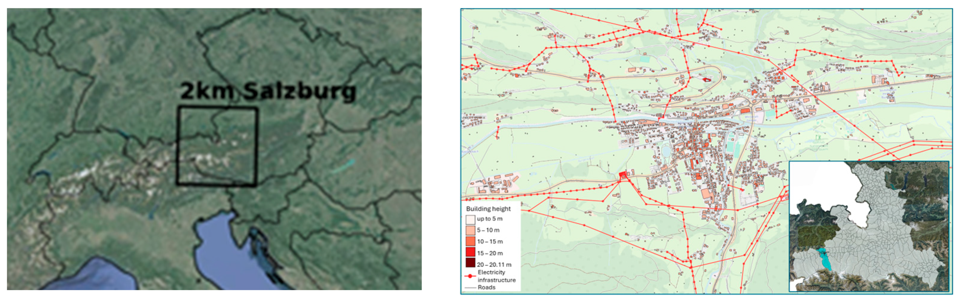
For representing future extreme precipitation and wind gust events, the convection permitting high-resolution regional climate model output computed within the ICARIA project [19] was used, see in Figure 1.

The COSMO-CLM (CCLM, version 4.8_19, [20,21]) was employed for dynamical downscaling of CMIP6 global climate projections covering the SSP scenarios 1-2.6 and 5-8.5, representing a climate scenario according to the Paris agreement (SSP126) and a worst-case scenario following a fossil fuel-driven future development scenario (SSP585) [15], and aligning with observed CO₂ emissions at the time the simulations were started [22]. It was driven by EC-EARTH3-Veg outputs, which are also used within the EURO-CORDEX simulations [23].

CCLM was developed and maintained by the COSMO Consortium (CLM-Community, www.clm-community.eu, accessed on 20 March 2026), an internationally coordinated scientific network dedicated to advancing Climate Limited-area Modeling. COSMO-CLM builds upon the operational COSMO weather prediction model of the Deutscher Wetterdienst [24] and solves the full set of primitive equations governing compressible flow in a moist atmosphere. The model incorporates comprehensive representations of key physical processes, including radiation, turbulence, land–surface interactions, and convection. Its numerical integration relies on a mode-splitting strategy that separates the governing equations into a longer time step for largescale and slowly evolving processes such as advection and physical parameterization tendencies, and a short time step specifically designed to capture rapidly propagating sound waves [25].

All simulations produced hourly output extending from 1981 to 2100. Wind speed was not verified, due to limited availability of suitable observation data [26] and because the focus within this work is to investigate the change in intensity and frequency of the occurrence of events, especially compound and consecutive events. For this task, we decided to not apply a bias correction because many methods applied during the adjustment also alter the climate change signal especially regarding precipitation [27]. To analyze the intensities and frequencies of precipitation and extreme wind, the 240 available years (1981–2100, 2 SSP scenarios) were used.

2.3. Verification and Analysis Criteria

To validate the model set-up, the CLM model was also initialized with ERA5 data covering the historical periods (1981–2010). The ERA5 reanalysis [28] developed by the European Centre for Medium-Range Weather Forecasts (ECMWF) was selected. The precipitation intensities are verified against the CHELSA [26] reanalysis dataset with a spatial resolution of about 1 km² (30 arcsec) and daily frequency which is used to evaluate the model’s skill in representing high-intensity events with the chosen set-up. Thus, the bias of maximum precipitation intensities is especially computed. The BIAS is used as it displays the systematic difference between the simulated and reference values. The BIAS was computed once for the whole domain, as well as for topographic heights above and below 1500 m to represent the impact of the topography on the modeled intensities. Further, a more detailed comparison of the downscaled simulations, the driving GCM and climatological observation data (CHELSA, 2.3) was performed in Bügelmayer et al. [19]. There, the model skill, due to its high spatial resolution with respect to mean temperature and yearly precipitation, was displayed.

2.4. Compound and Consecutive Events

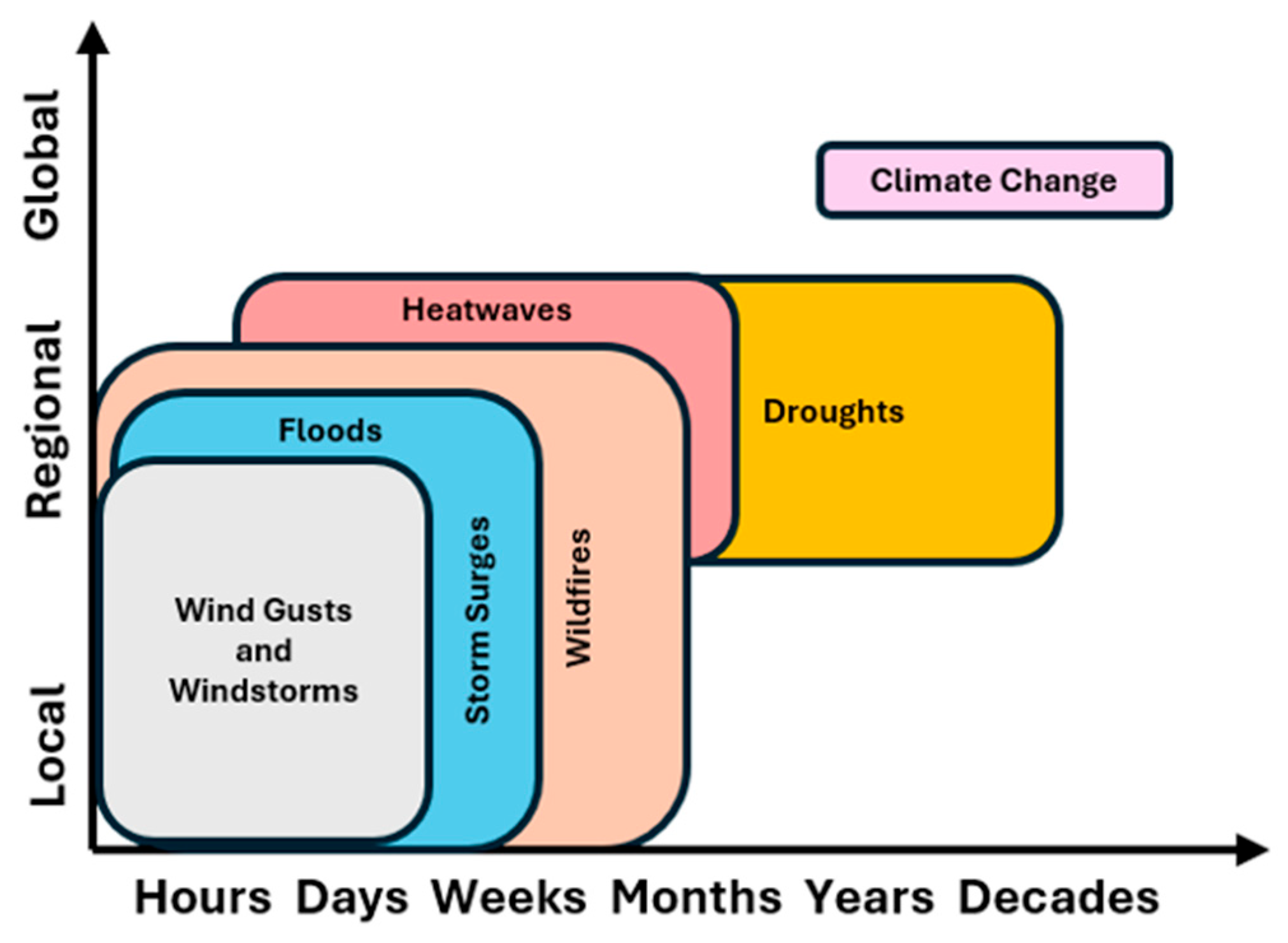
The modeling of compound events begins with defining both the spatial and temporal extents of the hazards of interest. Previous studies ([29,30]) have categorized a range of hazards according to these scales which have been referenced in the ICARIA project to aid in defining the boundaries of hazards being considered across the case studies (Figure 2).

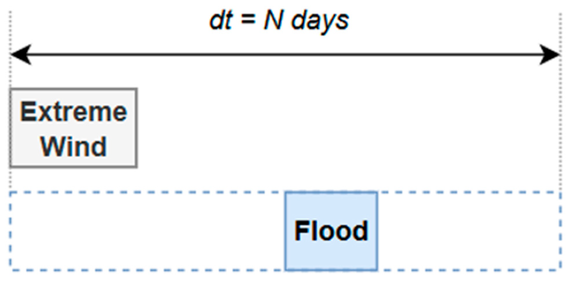
This study specifically focuses on the compound hazards of windstorms and flooding, which are prevalent in the Salzburg region and were prioritized during stakeholder engagement discussions. For these events, the probabilities of both compound coincident and consecutive events are being considered. Within the context of compound events, a crucial step is to define the time frame of which the secondary event must occur for it to be considered a compound event. Here, dt ranges from 0 (representing coincident events) to N days, where N denotes the maximum duration during which the antecedent windstorm may still influence the probability and/or magnitude of the subsequent flooding (Figure 3).

For consecutive events, we re-analyzed the daily joint probability of the maximum precipitation and wind gusts within an N-day window. Assuming everyday has the same likelihood of two hazards happening within the N-day slot, we can further determine the annual exceedance probability of event B occurring within N days of event A. With the climate data being at daily resolutions, the probabilities need to be converted to annual probability and the respective return periods based on the following steps, assuming the daily occurrences are independent events with same probability:

• Define the Joint Probability (P_joint): Determine the probability of event B occurring within N days of event A.

P(B within N days of A) = P_joint

2.

Define the Non-Occurrence Probability:

P(no event in N days) = 1 − P_joint

3.

Calculate the Annual Non-Occurrence Probability:

P(no event in year) = (1 − P_joint) ^(365.25-N)

4.

Determine Annual Exceedance Probability (AEP):

P(at least once per year) = 1 − (1 − P_joint) ^(365.25-N)

5.

Calculate Return Period (RP):

RP = 1/AEP

2.5. Bivariate Copulas for Climate Driver Dependencies

In contrast to single-hazard models, compound-hazard events can have a continuous range of values, for example, a 1-in-10-year compound wind and rainfall event could consist of high winds and medium-intensity rainfall, high-intensity rainfall and medium-strength winds, or a range of combinations in between. In scenarios where there are dependencies between the hazard drivers, these dependencies can be expressed via the use of copulas. Copulas are thus a mathematical function for modeling the dependencies between two or more random variables [31].

The selection of a copula for describing the dependency structure between datasets depends on their respective marginal distributions. For datasets that exhibit greater dependency within the mid-range, a Gaussian copula may describe the dependencies best, whereas for datasets showing stronger correlation at the extreme values, a Clayton copula may provide a more accurate depiction. Within this study, the Python (Version 3.13.) library “Copulae” [32] was used to analyze the marginal distributions of wind gusts and rainfall datasets and map their dependencies via a copula function.

Table 1. The AIC values of copula models (bold value indicates the best-fitting copula selected) and the KS statistic test of the selected copula.

Climate Scenario and Period		Gaussian	Clayton	Gumbel	Kolmogorov–Smirnov (KS) Statistic
					Precipitation		Wind Speed
					D Statistic	p-Value	D Statistic	p-Value
SSP1-2.6	1981–2010	−1095.33	−450.57	−1072.28	0.0020	1.0000	0.0032	1.0000
	2021–2050	−1122.56	−390.38	−1121.37	0.0020	1.0000	0.0033	0.9999
	2041–2070	−1082.85	−390.32	−1054.69	0.0020	1.0000	0.0032	0.9999
	2071–2099	−938.30	−303.02	−959.37	0.0020	1.0000	0.0032	0.9999
SSP5-8.5	1981–2010	−1095.33	−450.57	−1072.28	0.0020	1.0000	0.0032	1.0000
	2021–2050	−1077.97	−374.87	−1064.66	0.0020	1.0000	0.0032	0.9999
	2041–2070	−1113.89	−368.33	−1116.06	0.0031	1.0000	0.0018	1.0000
	2071–2099	−980.93	−286.68	−979.76	0.0022	1.0000	0.0034	0.9999

lists the calculated Akaike Information Criterion (AIC) of Gaussian, Gumbel, and Clayton copula of different climate scenarios and periods, while the bold values indicate the best copula fitting for estimating their daily joint probability of precipitation and wind gusts of each climate scenario period. The Kolmogorov–Smirnov (KS) statistics were further applied to check the goodness-of-fit of the selected copula.

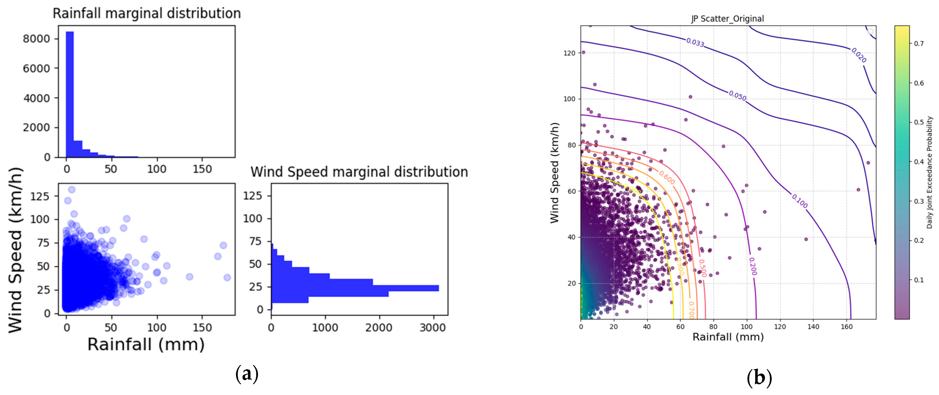
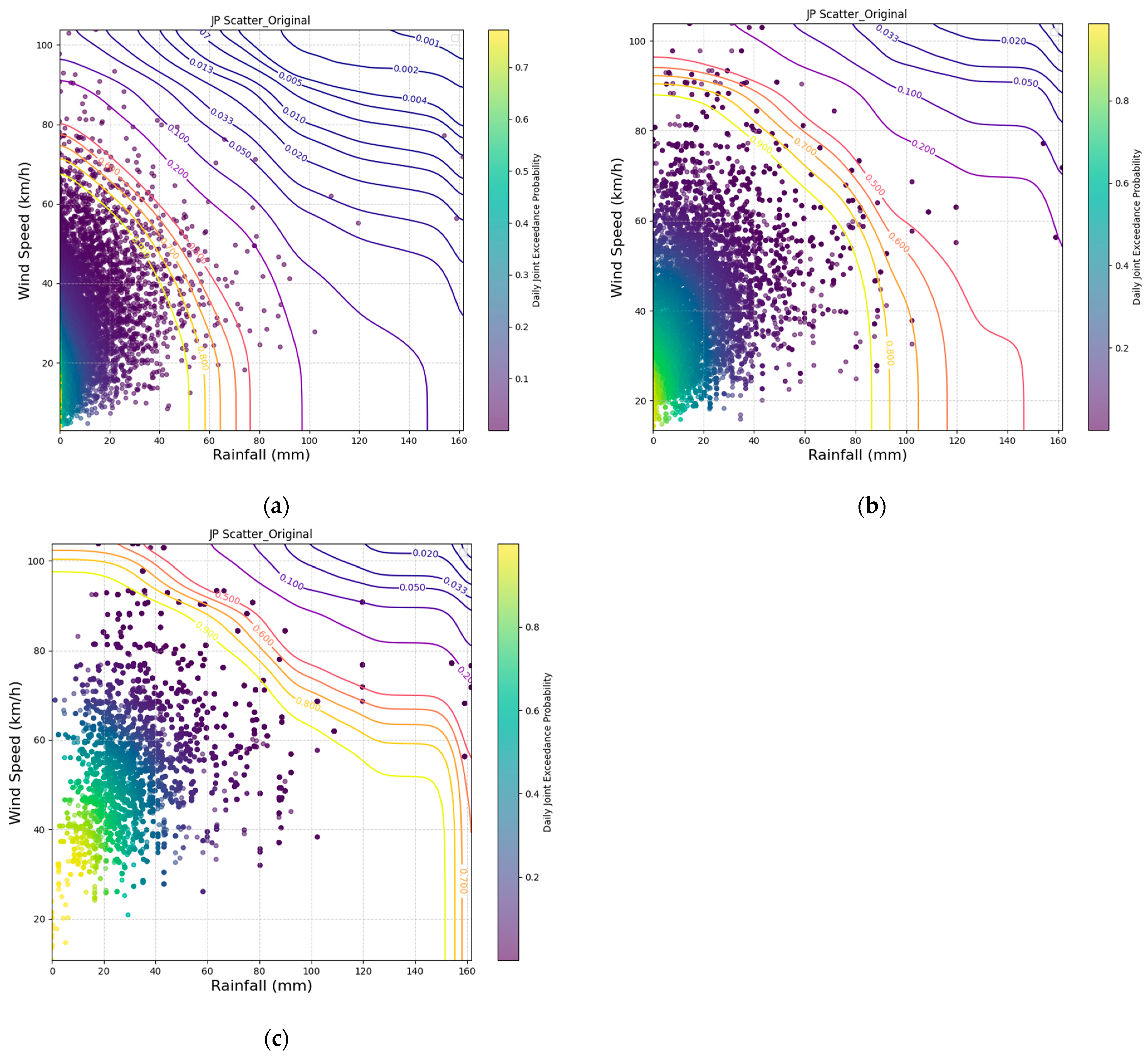
Figure 4a illustrates an example of the marginal distribution of daily rainfall and maximum wind speed of gusts for the SSP1-2.6 1981-2010 scenario. The Gaussian copula was found to be the best fitting (Table 1) and was applied to derive the joint probability of coincident (occurring on the same day) rainfall and maximum wind gust events. The scattered dots in Figure 4 represent the daily joint probability of the coincident events derived from the SSP1-2.6 climate projection data, while the contours illustrate the analyzed annual joint probability of daily rainfall and maximum wind gust combinations.

3. Results

The study examines how stakeholder input and state-of-the art climate model output is necessary in defining and consequently evaluating the occurrence of compound coincident and consecutive events that pose a threat to the community at focus. Thus, first the outcomes of the CoP are displayed, then followed by climate model results and finally the analysis of the events is presented.

3.1. Discussion with Stakeholders—Results CoP

In the second CoP, we discussed compound and consecutive events using two scenarios:

(1)

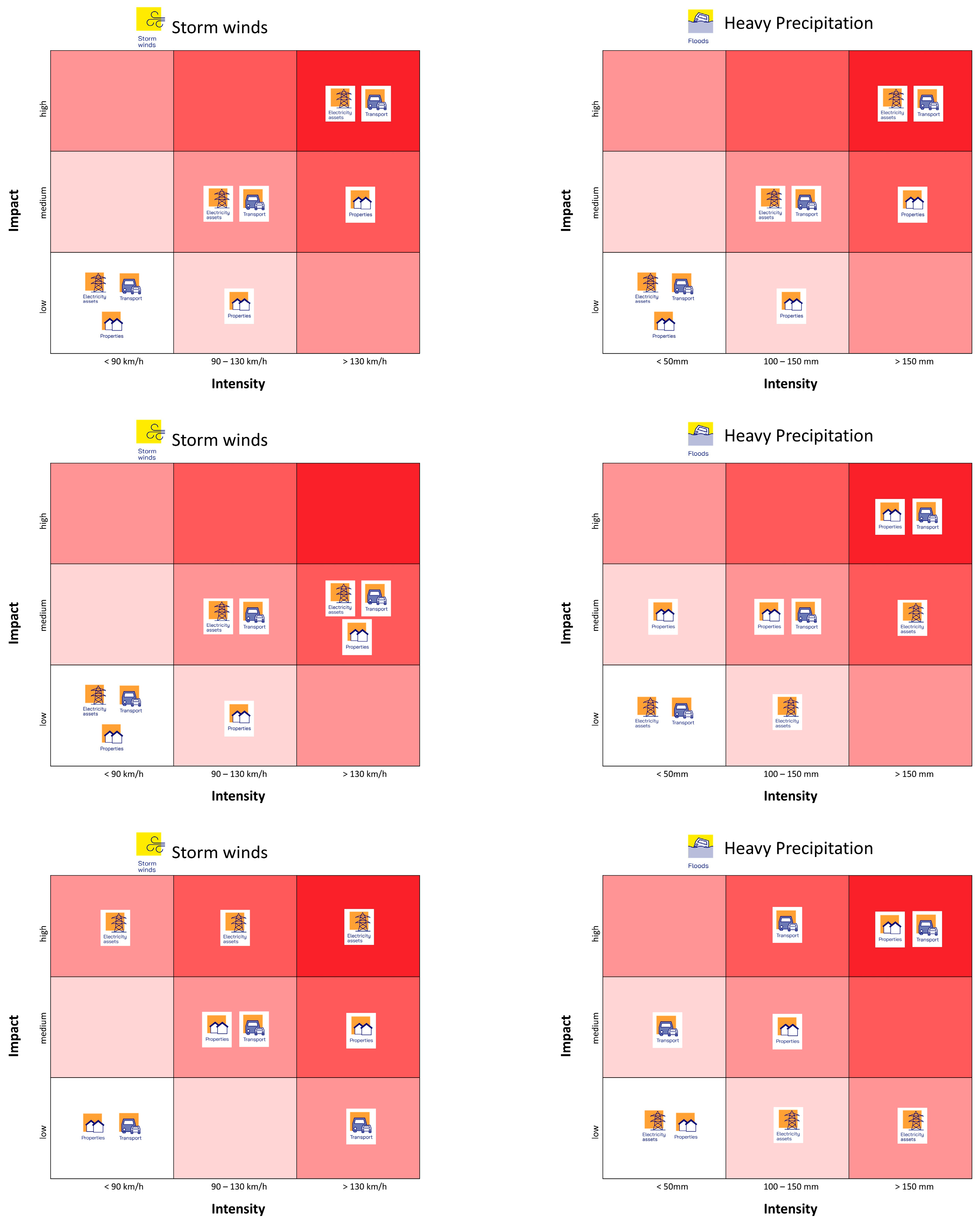
How severely will the assets “Electricity”, “Properties” and “Transport” be affected if (a) a storm is <90 km/h, 90–130 km/h or >130 km/h and (b) if the rain intensity is <50 mm/day, 50–100 mm/day, >150 mm/day?

Scenario 1 was defined as follows: A summer’s day during a warm spell, low soil moisture, location next to a stream in an urban area (high probability of flooding), localized rainfall, localized storm.

The x-axis of the following risk matrix shows the affectedness (little, medium, high) and the y-axis shows the wind speed. Three intensity ranges (little, medium, high) were chosen as this is a common classification scheme (three steps) and it allows us to define thresholds without representing too much granularity to specific speed values that are not reflected within the expertise of the local actors. In the CoP, the stakeholders formed three groups with 3–4 participants each for the discussion. The groups were formed at random, as the participants come from a variety of disciplines as described in 2.1 resulting in a broad range of expertise within the groups. Each group discussed both storm winds and heavy precipitation impacts.

Storm Wind Vulnerability: The stakeholder analysis reveals that wind-induced risk in the Salzburg region is characterized by a critical threshold between 90 and 130 km/h (Figure 5). While two groups adopted a more conservative stance, suggesting that structural damage on the electricity towers only becomes likely at speeds of 150 km/h, one group identified the electricity sector as the most critical point of concern, citing high affectedness even at speeds below 90 km/h. This discrepancy suggests that while physical structures may remain intact, the operational resilience of the power grid is perceived as highly fragile. A key qualitative insight discussed in the groups was the role of windthrow; stakeholders noted that the primary driver of infrastructure disruption is not the direct impact on assets, but rather the secondary impact of falling trees/timber on power lines and transport tracks. Consequently, for the Transport sector, the storm risk is viewed as a temporal cascade: initial blockages are manageable, but affectedness becomes medium or, respectively, high as the duration of the storm prevents rapid clearing and maintenance. Another insight discussed by the stakeholders was that when wind gusts reach around 130 km/h, most people stay at home, which means the impact on the transport system decreases again.

Heavy Precipitation: The risk perception for heavy precipitation is dominated by the 150 mm/day barrier, which all groups identified as a severe tipping point for “Properties” and “Transport” (Figure 5). Below 50 mm/day, stakeholders generally expect minimal impact on the discussed assets with only little effect on transport infrastructure. However, as intensities reach 100 mm, the Electricity sector is viewed as relatively robust against pure rainfall, and the Transport and Property sectors move rapidly into “medium-to-high” affectedness due to localized flooding. In the discussion, the identification of mudslides/landslides emerged as an impact of these hazards: at intensities exceeding 150 mm/day, the geological stability of the Alpine terrain is compromised, leading to impacts where mudslides, rather than just rising water levels, threaten both residential properties and critical infrastructure. This confirms that for the Salzburg region, extreme rainfall acts as a multi-hazard trigger that overwhelms standard flood protection once specific geological thresholds are crossed.

(2)

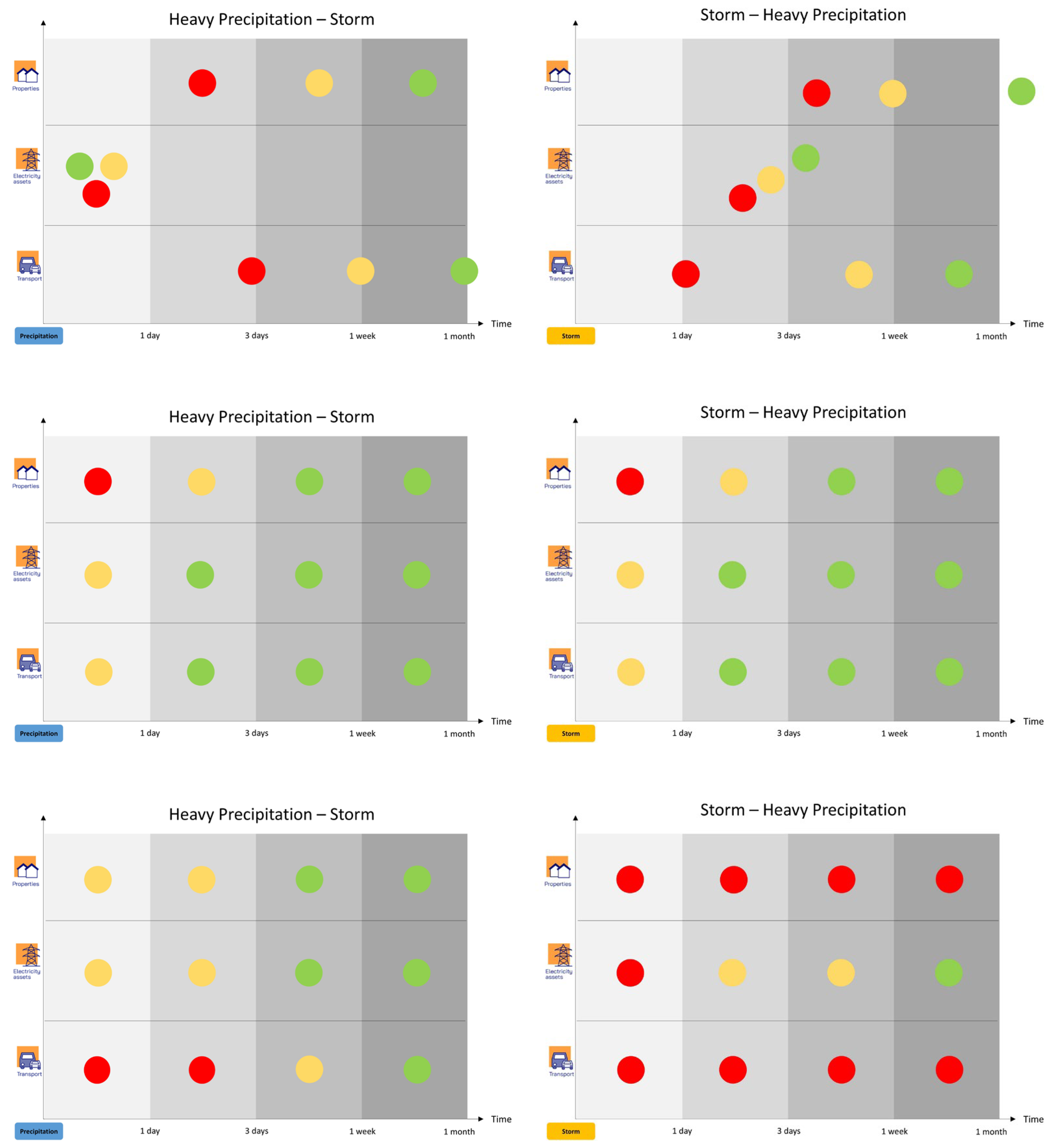
How long does it take for a subsequent event to continue having an impact before the original state (prior to the two events) can be restored? (a) How long does the region remain more vulnerable to rainfall after a storm has passed? (b) How long does the region remain more vulnerable to storms after a heavy rainfall event has occurred?

Scenario 2 was defined as follows: The extreme weather event under consideration has occurred and has already led to negative environmental impacts. The location is adjacent to a stream in a built-up area. High probability of flooding.

The x-axis of the risk matrix shows the time, and the y-axis shows the assets.

Heavy Precipitation Followed by a Storm: While one group remains optimistic, seeing a return to the original state within three to seven days, the others anticipate a little longer period of disruption. Specifically, “Transport” and “Properties” are flagged as the most vulnerable assets, with significant impacts remaining for up to three days and full restoration often taking one month. This suggests that saturated terrain and potential landslides create a highly sensitive state where even moderate winds can trigger systemic failures in infrastructure that would otherwise remain stable (Figure 6).

Storm Followed by Heavy Precipitation: The “Storm–Heavy Precipitation” scenario reveals stronger systemic concerns. One group presents a severe outlook, where the assets “Properties” and “Transport” remain at maximum vulnerability for over a month due to compromised roofing and debris-clogged drainage. While one group sees a gradual recovery over three weeks, all groups agree that the initial storm damage creates a weak system where subsequent rain causes disproportionate harm. “Electricity” assets prove most resilient across all groups, generally stabilizing within one week, though the overall “recovery window” for the region is dictated by the much slower restoration of the built environment.

Overall, the “Heavy Precipitation–Storm” scenario is perceived as less catastrophic than the other way around. This could be because heavy rain events often trigger an immediate high-alert status among disaster management teams, acting rapidly, and the subsequent wind event occurs within a system that is already fully mobilized. In contrast, an initial storm causes structural “openings”—such as damaged roofs or blocked roads—that allow subsequent rain to cause compounding, unmanageable interior and secondary damage before repairs can even begin (Figure 6).

To summarize, the stakeholders, although coming from different disciplines, all regularly encounter extreme events in their daily operations and are therefore well-positioned to evaluate the relevant thresholds. All groups identify one day as a critical time frame, for at least one asset, in both scenarios. However, their specific disciplinary backgrounds influence their perspective on event duration: stakeholders responsible for critical infrastructure tend to focus on short-term impacts, whereas those operating also in rural sectors also account for longer durations. Up to one week is identified as critical for at least one asset by two groups and impacts up to 1 month are still stated as critical by one group. We therefore decided to define the time windows 1 day, 7 days and 1 month to account for the fact that—depending on the asset and its location within Salzburg—it may be affected by storm and more vulnerable towards extreme precipitation for time frames up to one month.

3.1.1. Climate Simulations—Validation of Extreme Precipitation Events as Displayed by CLM

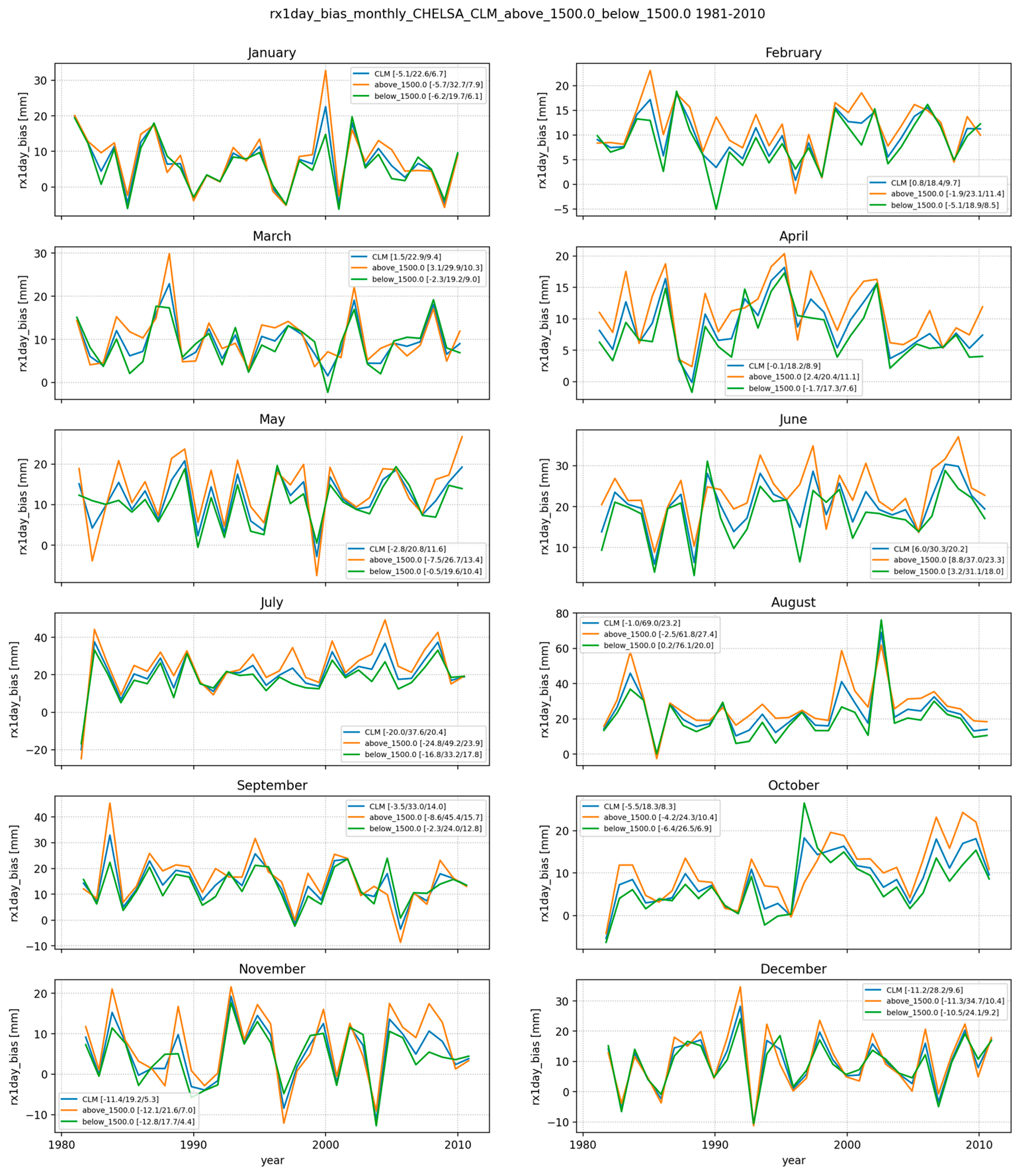
Regarding the past climate, the verification of extreme precipitation, as represented by the indicator of maximum precipitation per day (RX1 day), displays higher intensities in CLM than CHELSA, with maximum BIAS occurring during summer due to convective events (Figure 7). From October to May, the simulated intensities deviate from observation by about −10 to 20 mm, with mostly higher intensities simulated than observed. During summer months (June to September) the BIAS increases, with maximum overestimation of up to 80 mm/day occurring during August at higher altitudes (above 1500 m, Figure 7). The BIAS displays overall higher values in higher altitudes, with the strongest overestimation during August, with a few exceptional events. In general, the BIAS of CLM compared to CHELSA displays an overestimation in the range of 0–20 mm, with a few summer events that display higher intensity overestimation. Nonetheless, the performance of the model displays satisfactory results to be used for assessing future climate conditions under different emission scenarios.

3.1.2. Future Climate Conditions

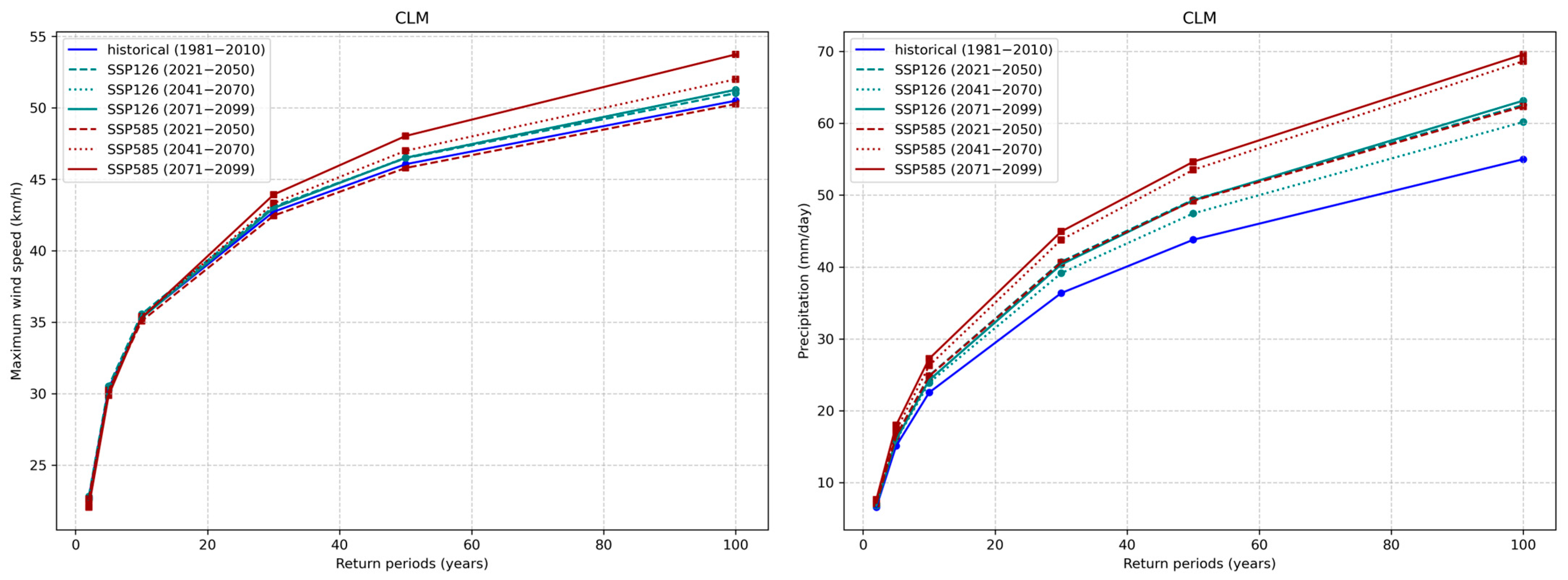
For wind gusts, no telling increase is seen for future periods and low emission scenario compared to the historical time period; independent of the return period, a slight (5 km/h) increase is seen towards the end of the century in the SSP5-8.5 simulation (Figure 8). Yet, maximum precipitation intensities per day increase for all return periods, with an increase of ~10 mm for both emission scenarios, except the late future (2071–2099), which displays up to 20 mm/day increase (Figure 8). These values represent an increasing intensity in future extreme precipitation events, as assessed over 30-year time periods.

3.2. Compound and Consecutive Events

The daily joint exceeding probability, the annual exceeding probability of compound coincident and consecutive rainfall and windstorm events, as represented by wind gusts, under the SSP1-2.6 1980–2010 scenario are analyzed. For compound coincident events, the 0.5 annual joint probability (i.e., equivalent to a 1-in-2-year return period) has a maximum daily rainfall up to 78 mm and a wind speed up to 80 km/h under baseline scenarios (Figure 9a). However, these are conditions when one factor is approaching an extreme value when the other factor is close to zero, therefore representing single rather than multi-hazards. Only within and beyond the 100-year return period (0.01) do single events occur that display extreme precipitation (>150 mm/day) and more intense wind gusts (>70 km/h), although it has to be kept in mind that wind gusts <90 km/h do not represent a threat to the assets investigated within this study.

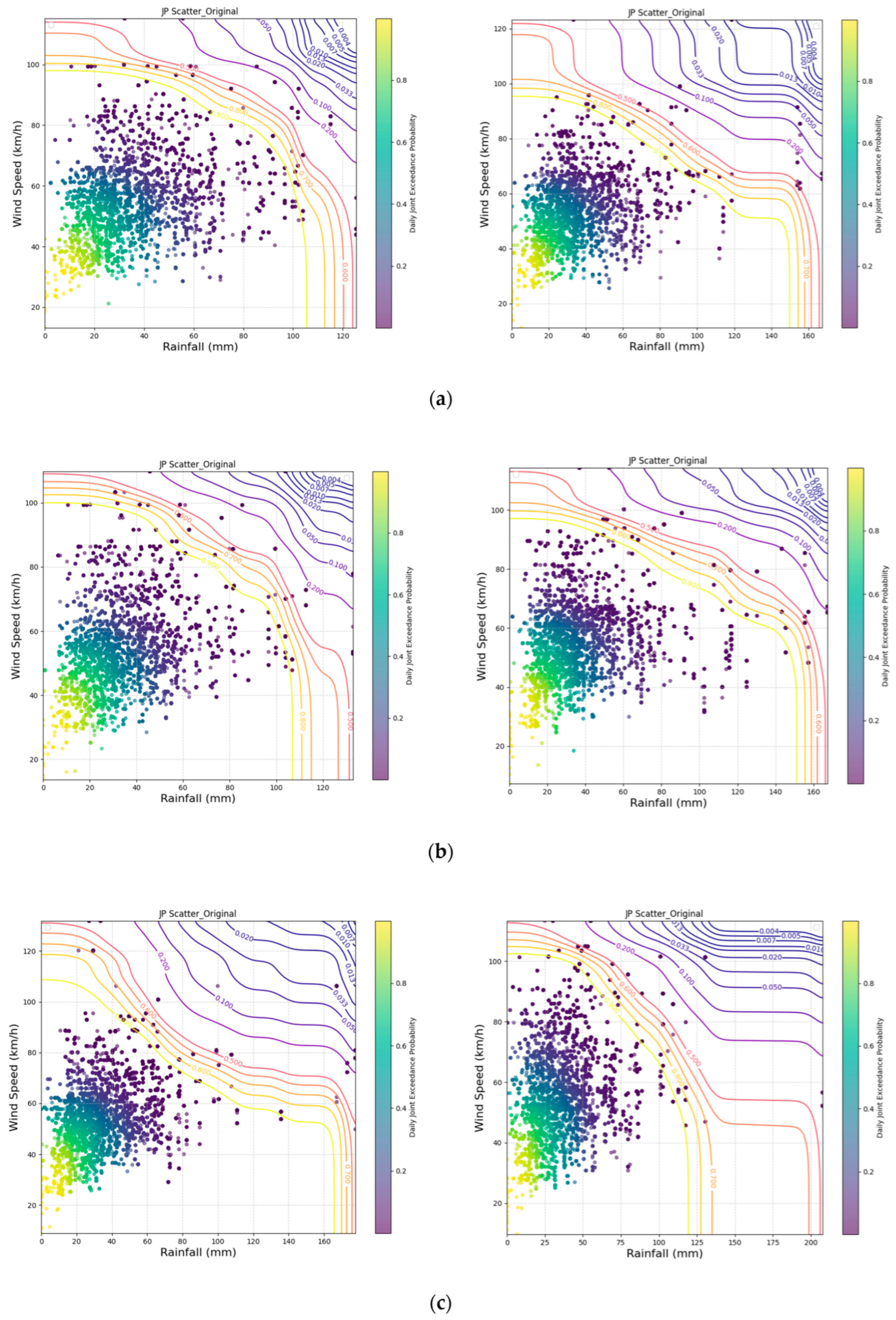
For consecutive events within a 7-day time window (Figure 8), rare events that display strong wind gusts (90–100 km/h) and intense rain (>50 mm/day) occur with a 0.5 annual joint probability. For consecutive events within a 30-day time window, the ranges of both parameters for 0.5 annual joint probability further expand to over 160 mm daily rainfall and over 100 km/h wind speed, or—as the focus is on multi-hazards, the combinations of 60 mm daily rainfall and 92 km/h wind speed (crossing the lowest thresholds identified by stakeholders)—100 mm daily rainfall with 78 km/h wind speed.

The results also show that the larger time window will reduce the combinations of variables to the maximum values within the time span, hence reducing the data points and increasing the daily joint exceeding probability of combinations. The results clearly demonstrate that the time window selection significantly affects estimations of joint probability of compound events.

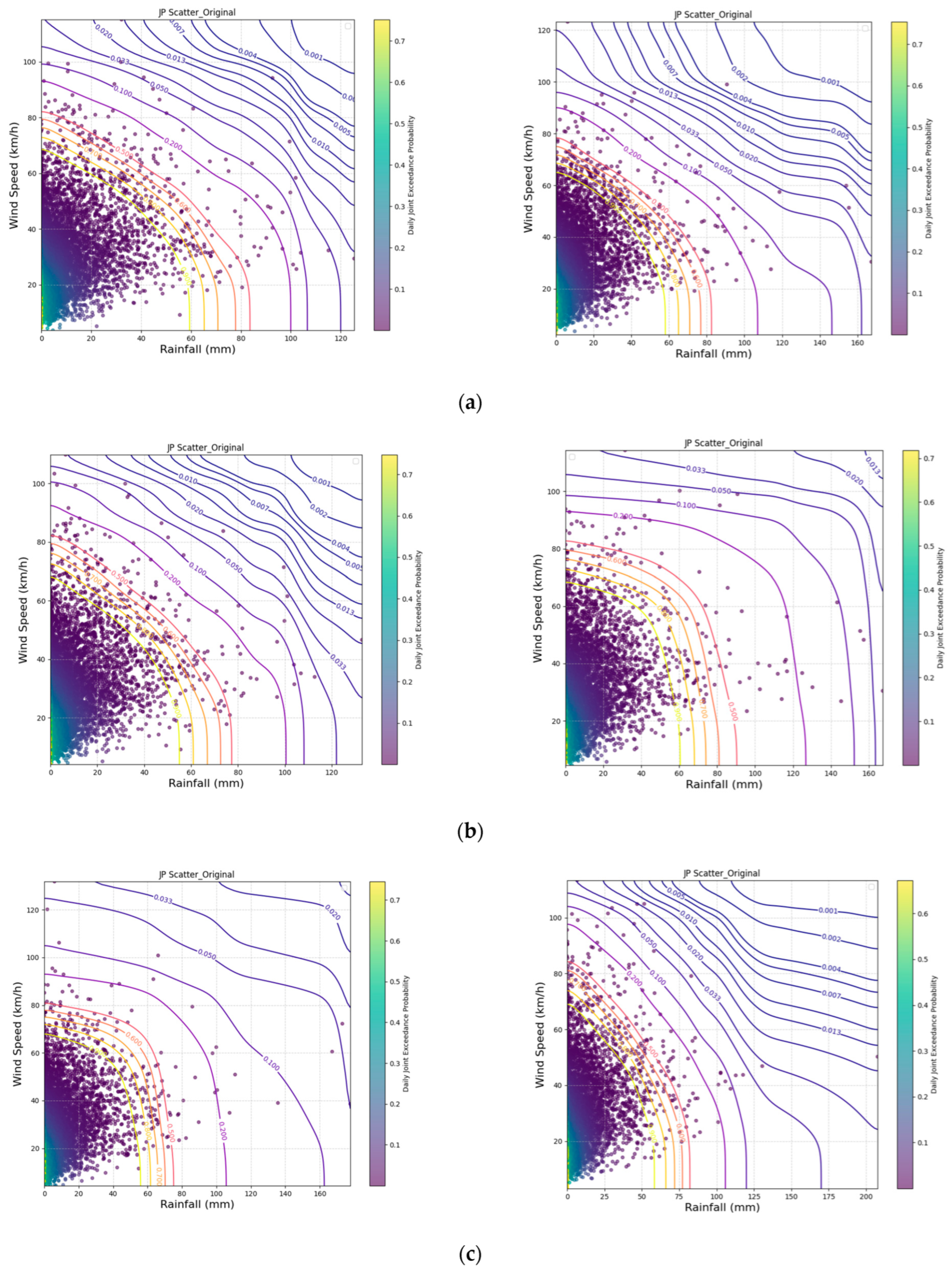
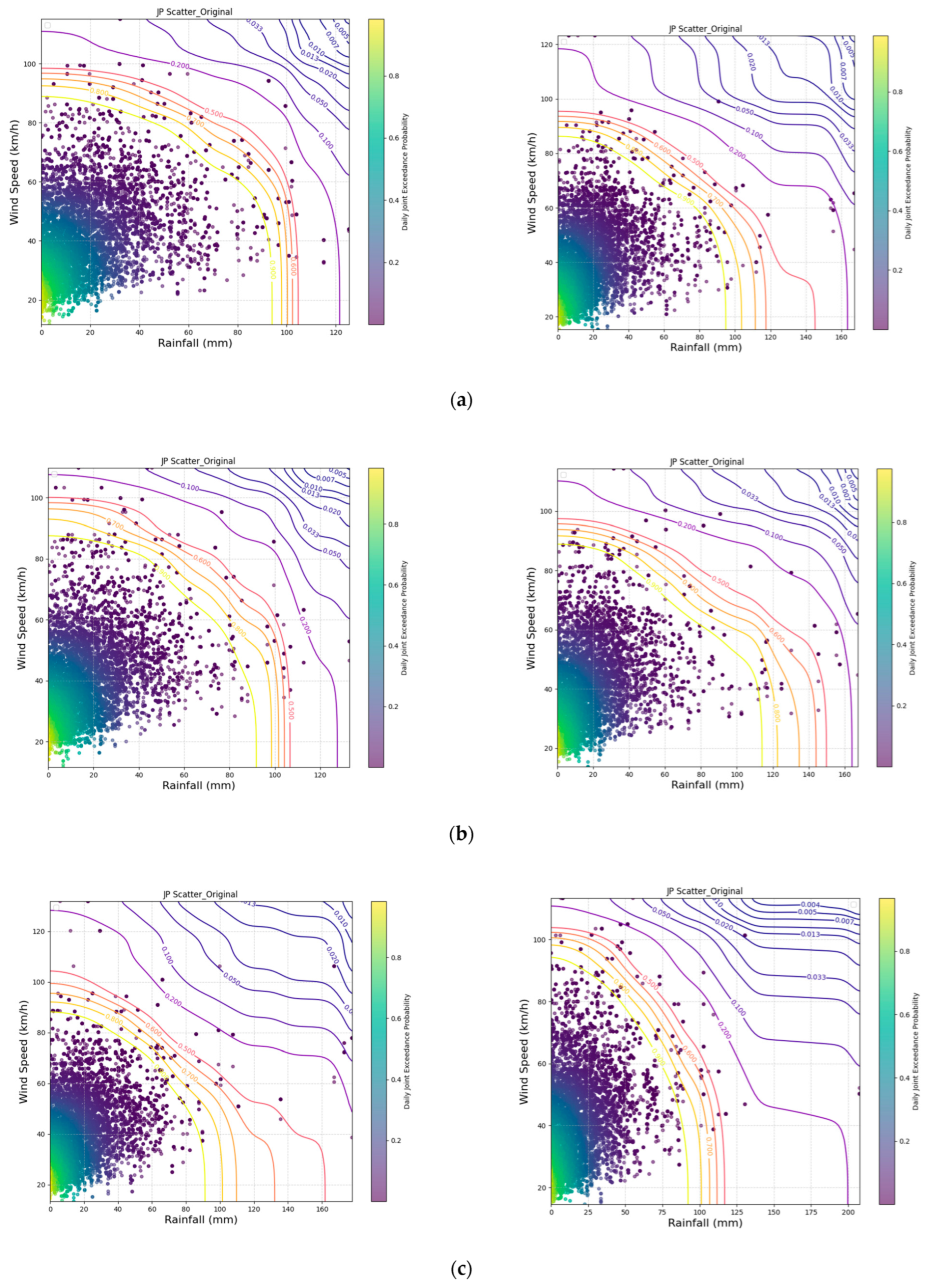
Figure 10, Figure 11 and Figure 12 present the joint probability analysis of compound coincident (Figure 10) and consecutive (7 days, Figure 11; 30 days, Figure 12) rainfall and windstorm events under the SSP1-2.6 and SSP5-8.5 scenarios. The intensities of rainfall and wind gusts in those scenarios are greater than the baseline scenario such that variable axis ranges are used to display the contours properly. The results are similar to the baseline scenario in the sense that the larger the time window, the higher the joint probability of both events occurring. The value combinations of variables with 0.5 annual joint probability in the baseline scenarios will have over 0.9 annual joint probability under the SSP1-2.6 and SSP5-8.5 scenarios, indicating higher frequency or increased severity and impact of future compound coincident and consecutive events. Especially towards the end of the century and SSP5-8.5, the precipitation intensities of single events increase, representing a maximum rainfall of 200 mm/day, and therefore an increase of about 30%.

4. Discussion

The aim of the presented study was to present first insights into relevant thresholds representative of high-impact events in a case study (Salzburg) with respect to daily precipitation and wind gusts, the time that is needed to ensure full functionality of the assets in focus again and how often compound coincident (occurring within 1 day) and consecutive extreme events occur within the time window identified. To answer these questions, a combined approach of stakeholder input, high-resolution climate model output and an analysis suitable for compound and consecutive extreme events was taken. Thereby, it was gathered that the intensity of extreme precipitation and wind relevant to the investigated assets (properties, transport, electricity) was assessed similarly between the involved stakeholders, while the recovery time was estimated quite differently, with time frames ranging from one to a few days, up to one month. These different assessments by local stakeholders indicate that the time assessment depends on professional background and personal experience. For instance, people that are mainly connected to infrastructure of great importance are used to having maintenance happening within a few days, while representatives of rural areas have experienced time frames of weeks or even months. The current stakeholder group consisted of about 15 people, all well experienced with the local impacts of extreme events but with different backgrounds; thus, having more representatives especially for defining the time frame would be beneficial. It must be acknowledged that a different stakeholder group might have reached different conclusions. Future research is required to further refine these thresholds, particularly concerning the temporal dimensions of the recovery windows, to ensure broader applicability and robustness. Additionally, for future multi-hazard assessments, a more detailed distinction between type of asset (critical, location) and, overall, a broader stakeholder group from different regions is suggested to reduce uncertainties in stakeholder responses. Further, the insights gained from the expert-based assessments would benefit from quantitative analysis based on data, in case it is available.

Regarding the intensity of precipitation and wind gusts, it is important to consider that the data used represents potential future conditions but is only based on one model; thus, to strengthen conclusions, the study should be enhanced with additional model data, when available. Within Maier et al. [33], regional downscaled projections of different emission scenarios, including the ones presented in this paper, were put into context with two CMIP6 ensembles for the scenario SSP126 and SSP370; see Figure 7. Compared to the SSP370 ensemble, that represents a lesser increase in CO₂ emissions, our model’s temperature change is along the upper range of the ensemble’s spread especially towards the end of the century. Even though the model put into context of a CMIP6 GCM ensemble showing its climate change signal in temperature behaves as expected and in accordance with the other models of the ensemble, one has to keep in mind that this conclusion cannot be made for precipitation or wind gusts because these parameter’s climate change signal can behave differently for each model [34]. Therefore, the conclusions regarding changes in wind and precipitation cannot be generalized. A comparison with a EURO-Cordex RCM ensemble would help in this regard, but at the time this paper was written, the CMIP6 EURO-Cordex ensemble was still not available. Nonetheless, the model simulations were performed on convection permitting scale, therefore resolving convective processes and enabling insights difficult to draw from coarser projections [35]. Further, the model validation displays satisfactory results for the historical period, since the observed bias of extreme precipitation might also be related to the fact that rain rates in mountainous regions as depicted by observation datasets are prone to errors and undercatchment can amount up to 80% [36]. Further, Outten and Sobolowski [37] found an increase in wind speed per return period, especially towards the end of the century, when analyzing 15 EURO-Cordex simulations, being in line with the findings of increasing intensity compared to the baseline scenario. Bloomfield et al. (2023) [38] showed strong correlation of wind gust and rainfall events ranging from 0.6 to 0.8 for daily and seasonal scales within Great Britian with peaks around 10 days between events. Extending their analyses over the wider Europe area, they showed that countries in central and northern Europe that experience frequent extra-tropical cyclones observe high correlation between windstorms and flood events at weekly to monthly timescales. In Owen et al. (2021) [39], when examining the temporal offset between precipitation and winds across Europe, they highlight that whilst there is an extremal dependence between winds and rain in certain regions either surrounded by or on high elevation, there is a significant time separation between them as extreme precipitation near elevated topography are further away from cyclone centers.

5. Conclusions

As climate change alters the intensity and frequency of extreme events, compound coincident and consecutive extreme events are increasingly recognized as critical drivers of climate risk as they can amplify impacts beyond what would be expected from individual hazards considered in isolation. Therefore, the understanding of their occurrence under present and future climate states is key for sustainable adaptation and decision-making.

Within this study, we present a promising approach combining stakeholder integration with convection permitting model simulations and copula-based analysis of compound coincident and consecutive events to gain better insights into relevant multi-hazards for Salzburg. The implemented Community of Practice (CoP) identified extreme wind gusts and extreme precipitation as key hazards for the region. Since data on hazard intensities that relate to damage for different assets (buildings, transport and electricity network) as well as on the time for repairs were not available, the integration of the local expertise presented a valuable approach for a first assessment. Further, the involvement of local actors facilitated the uptake of the presented results. The stakeholders identified suitable intensity thresholds for precipitation (low: ~50 mm/day; medium: 100–150 mm/day; high: >150 mm/day) and wind gusts (low: 90 km/h; medium: 90–130 km/h; high: >130 km/h). The time it took until all assets considered were repaired was indicated to be between 1 and 7 days, and in specific cases also up to 1 month. These defined the thresholds used for the joint probability analysis.

The convection permitting model projections display only a limited increase in wind gusts and a stronger one in precipitation intensities from the historical to the future periods, with the clearest signal within the high emission scenario (SSP5-8.5 vs. SSP1-2.6). This is represented by the intensities of specific return periods, where maximum rain intensities per day increase for all return periods (up to 100 years) within all emission scenarios. The highest increase of about 30% is seen in SSP5-8.5 in 2071–2100.

Further, the joint probability analysis displays that the intensity of compound coincident, as well as those that are consecutive within 7 days and consecutive within 1 month, increase by ~30% between each time window. The annual exceedance probability shows that, for instance, for the near future, intensities occur as compound coincident about every 10 years, might occur every other year within a 7-day window, and even yearly within a 30-day time frame.

Overall, this study presents the potential of an inter- and transdisciplinary approach in regional climate multi-hazard assessment and related impacts, which are gaining importance for future planning and adaptation strategies.