Impacts of Land Use Patterns and Associated Thresholds on Seasonal Water Quality Dynamics in a Typical Watershed of Qinling Mountains, China

Abstract

Land use and landscape patterns strongly influence water quality and are critical for ecological conservation within watersheds, as well as for effective water resource management. This study analyzed water quality data collected from 11 monitoring sites in the Minjiahe Watershed of Qinling Mountains, China. Redundancy analysis was used to analyze the impact mechanism of multi-scale landscape patterns and land use on seasonal water quality changes, while non-parametric change point analysis was used to quantify the key landscape thresholds that lead to sudden changes in water quality. The results indicated that the concentrations of ammonia nitrogen, available phosphorus, and total nitrogen in the river water were significantly higher during the rainy season than during the dry season (p < 0.05), representing increases of 18.93%, 30.33%, and 37.52%, respectively. The dissolved oxygen levels were 27.76% higher in the dry season than in the rainy season (p < 0.05). Landscape metrics at different spatial scales can strongly explain the spatiotemporal changes in water quality, with an explanatory rate exceeding 76%. The interspersion and juxtaposition index of forestland (IJI_for), largest patch index of forestland (LPI_for), landscape shape index of residential land (LSI_res), and percentage of landscape of farmland (PLAND_far) are the main factors affecting seasonal changes in water quality. Small and discontinuous grasslands did not significantly affect water quality. To effectively mitigate the impact of landscape patterns on water quality, the following thresholds are suggested as effective management targets: at the sub-watershed scale, IJI_for < 80% and LPI_for > 94%; at the 150 m buffer scale, LSI_res < 8 and PLAND_far < 8%. These determined thresholds can be used as indicators for landscape planning to reduce the risk of water quality degradation. The research results provide valuable insights for sustainable land use and multi-scale landscape planning, thereby informing strategies to enhance water quality.

1. Introduction

Clean water resources have been recognized as a key driver of human societal development. As the primary form of surface water, rivers are essential to social progress, environmental protection, and agricultural productivity [1]. Water quality directly impacts public health security and sustainable agricultural development, serving as a critical indicator for assessing the overall health of ecosystems [2]. In recent years, the degradation of river water quality driven by both natural factors (e.g., hydro-meteorological, topography, and soil) and anthropogenic influences (e.g., urban expansion, agricultural, and industrial emissions) has been increasingly observed [3,4]. The landscape pattern, a multidimensional construct shaped by both natural and human elements [5], significantly influences hydrological processes and the transport and deposition of terrestrial nutrients, such as nitrogen and phosphorus, into river systems [6,7]. Therefore, understanding the relationship between landscape indicators and water quality is essential for enhancing water resource management and informing land use planning [8]. Land use practices profoundly affect watershed hydrology and nutrient dynamics [9,10,11]. Specifically, urbanization alters surface hydrology and increases pollutant runoff, exacerbating eutrophication and water degradation [12]. Agricultural activities are often the main cause of nitrogen and phosphorus pollution [13], while forests and natural vegetation play an ecological role in mitigating pollutant inputs [14]. With the advancement of landscape ecology, landscape configuration has served as a robust framework for quantifying land use structures and analyzing spatial landscape patterns. Current research integrates both land use composition and spatial configuration to evaluate how patch size, shape, and distribution influence aquatic environments [15,16].

Extensive research has demonstrated that the influences of land-use configurations and landscape patterns on watershed water quality are scale- and watershed-dependent [17,18], highlighting the necessity to determine critical thresholds for effective watershed management. To address this, change detection techniques are widely employed to capture nonlinear responses and abrupt ecological transitions that conventional linear analyses often fail to detect [19,20,21]. Among these, non-parametric change point analysis (nCPA) was applied in landscape–water quality studies, it identifies statistically significant thresholds directly from empirical data without requiring a predefined functional form [22,23]. Compared with parametric approaches, such as piecewise or segmented regression, which require the number or approximate location of breakpoints to be specified in advance, nCPA provides greater flexibility for complex ecological datasets [24,25]. Bayesian change point analysis has also been used to detect shifts in environmental systems and offers probabilistic estimates of thresholds, but its results can be sensitive to prior assumptions and computational settings, nCPA maintains high sensitivity to abrupt ecological boundaries while avoiding the distributional assumptions required by parametric approaches [26]. Furthermore, machine learning methods such as random forest can rank the importance of landscape predictors but often fail to produce explicit threshold estimates, limiting their direct utility for establishing nutrient or pollution concentration targets [27,28]. While generalized additive models are capable of flexibly fitting nonlinear relationships, they do not provide statistically defined breakpoints, and their smoothing parameters may obscure the detection of sudden ecological transitions [29,30]. By directly locating change points from empirical data without prespecifying functional forms, nCPA offers a more transparent and data-driven framework for identifying critical thresholds in landscape-water quality studies. Additionally, nCPA can be combined with bootstrap resampling to quantify uncertainty around threshold estimates, which enhances its robustness for management applications [31,32]. This combination of distributional flexibility, explicit breakpoint localization, and uncertainty quantification makes nCPA particularly well-suited for informing threshold-based management decisions in complex socio-ecological systems.

In recent years, the abrupt relationship between landscape patterns and water quality has been increasingly recognized, often referred to as landscape thresholds or mutation points [33,34]. A landscape threshold typically refers to a critical value at which a water quality index exhibits an abrupt response to specific landscape indicators. Beyond this threshold, water quality tends to degrade rapidly as landscape characteristics shift. Identifying such thresholds is critical for effective landscape management and the protection of water resources in river watersheds [35,36]. Previous studies have demonstrated that under certain spatial configurations and proportions, the impacts of various land use types such as urban, farmland, and forest on nitrogen and phosphorus pollution, eutrophication, and water quality degradation may exhibit abrupt shifts. For instance, when forest coverage in agricultural regions falls below 47% or the edge density of wetlands drops below 36 m/ha, nutrient concentrations and eutrophication risks tend to increase significantly [37]. Similarly, when urban land patch density exceeds 30–40 patches per 100 ha, the risk of pollutant migration is significantly elevated [38]. Therefore, the selection of appropriate statistical models is essential for threshold identification. Among these, non-parametric point-of-change analysis has demonstrated high accuracy and practical applicability in detecting mutation points between water quality parameters and landscape metrics [39,40,41,42]. By integrating spatiotemporal scale analysis with mutation detection, the thresholds of key landscape indicators across different scales can be evaluated. In turn, a scientific basis can be provided for the development of more effective water quality management strategies and the establishment of ecological security thresholds in river watersheds.

The Danjiang River Watershed, characterized by abundant water resources, is a key supplier for China’s South-to-North Water Diversion Project [43]. Since 2000, the watershed has implemented key ecosystem restoration efforts, namely the “Returning Farmland to Forest and Grassland Project” and the “Natural Forest Protection Project” [44]. These initiatives have altered watershed characteristics, surface morphology, and river hydrology, thereby significantly enhancing the regional ecological environment. However, with ongoing socioeconomic development and population growth, water sources continue to face increasing pressure from rising water demand and intensified human activities, which poses new challenges to the protection of water quality in the watershed. Minjiahe River is a secondary tributary of the Danjiang River. It is an important water source area upstream of the Danjiangkou Reservoir and a typical river watershed for vegetation restoration and slope-to-ridge transformation in Shaanxi Province. Against this backdrop, ensuring water quality while promoting ecological restoration has become a pressing issue requiring urgent attention. To address this, the present study focuses on the Minjiahe sub-watershed, located at the source of the Danjiang River, to investigate the effects of landscape indicators on water quality. Accordingly, the present study was designed with two primary objectives: first, to assess how variations in land use and landscape configuration at different spatial scales affect seasonal dynamics of water quality; and second, to ascertain the spatial scale at which landscape patterns exert maximal influence on water quality, while also quantifying the threshold points corresponding to abrupt shifts in key landscape indicators.

2. Materials and Methods

2.1. Study Area

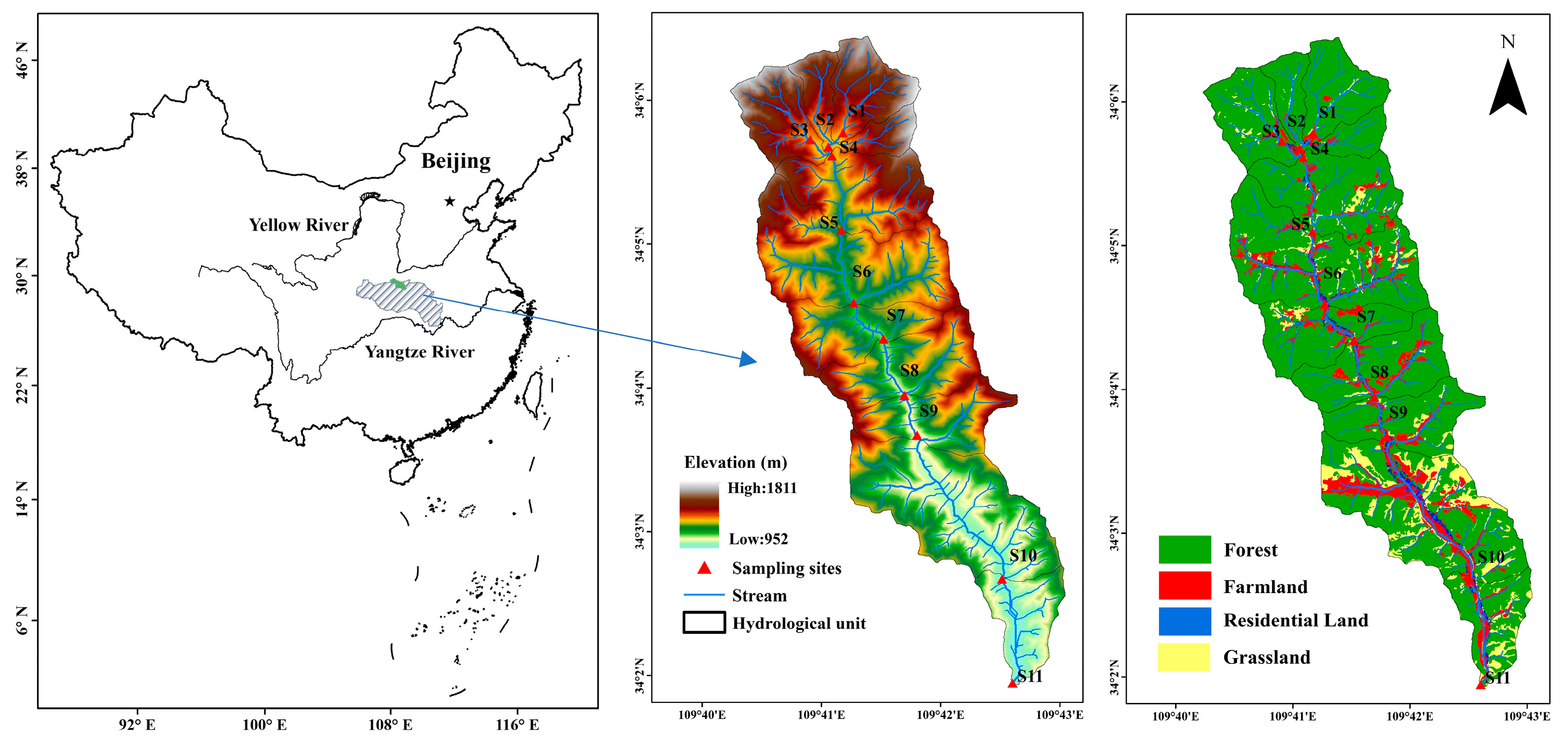
The study area is located in the Minjiahe Watershed of Shaanxi Province, China (109°40′11″–109°43′4″ E, 34°1′58″–34°6′29″ N, Figure 1). As a secondary tributary of the Danjiang River, spans a total length of 9.7 km and a drainage area of 15.04 km². The watershed is situated in the transitional zone between the warm temperate and northern subtropical regions and features a mild climate, abundant solar radiation, sufficient precipitation, and four distinct seasons [24]. The mean annual temperature ranges from 8.3 °C to 18.7 °C, with a multi-year average of 10.3 °C. Annual precipitation varies between 600 mm and 1125 mm, averaging 890.4 mm, with the majority occurring between June and September. The average flow rate values during the dry season and the rainy season are 0.78 m³/s and 1.23 m³/s in 2025, respectively. The highest elevation is 1811 m and the lowest is 952.3 m. Soil types vary significantly, mainly including stone slag soil, mountain brown soil, and silty sand soil. Forest land, farmland, grassland, and residential land are the main land use types.

2.2. Data Preparation

According to field conditions such as stream length and topography, 11 stream water quality sampling sites numbered S1–S11 were set up (Figure 1). Water quality samples were collected during 2020–2021 in an average cycle of 15 days, a total of 825 water samples were collected. Dissolved oxygen (DO) and electrical conductivity (EC) were measured in situ using an HQ30d water quality monitor (HACH, Loveland, CO, USA). At each sampling event, three replicate water samples (500 mL each) were obtained at each site using polyethylene bottles, and subsequently handled under controlled conditions, including labeling, transport to the laboratory, and storage at <4 °C. Total phosphorus (TP), orthophosphate (PO₄^3––P), total nitrogen (TN), and ammonia nitrogen (NH₄⁺–N) were analyzed using an Auto Discrete Analyzer CleverChem 200 (DeChem-Tech, Hamburg, Germany) within 24 h of collection. Samples collected between June and September were classified as rainy season samples, while the rest were dry season samples.

Landscape patterns were analyzed at two scales: sub-watershed and 150 m riparian buffer scales. The sub-watershed scale encompasses the entire catchment area upstream of each sampling point [45,46]. Because the farmland in the watershed is concentrated within a 150 m on both sides of the riverbank, a 150 m riparian buffer scale was chosen, which is a strip extending 150 m to the left and right banks of the river, with bounded by the sub-watershed. Firstly, a 5 m resolution digital elevation model (DEM) was used to delineate the catchment area for each sampling point at sub-watershed and 150 m buffer scales using ArcGIS 10.2 software, and the watershed is of a narrow and elongated shape. Then, land use data at various spatial scales were derived through intersection overlay analysis using ArcGIS 10.2.

The digital elevation model is sourced from the Hydrology and Water Resources Center of Shaanxi Province. The land use data is sourced from Google Earth imagery, dated 1 July 2020, with a resolution of 0.247 m. Based on the field conditions of the study area, there are mainly large areas of forests and grasslands, as well as farmland and residential land on both sides of the riverbank. Therefore, land use classification can be accurately and quickly completed through manual visual interpretation. The image is based on the WGS84 geographic coordinate system, and manual visual interpretation is completed in ArcGIS 10.2. Randomly generate 80, 50, 50, and 20 validation sites in forest land, grassland, cultivated land, and residential land based on the size of each land use area. Use confusion matrix (

Table 1. Accuracy evaluation of confusion matrix.

	Forest	Grassland	Farmland	Residential Land	Sum	User Accuracy
Forest	70	2	0	0	72	97.22%
Grassland	6	45	3	0	54	83.33%
Farmland	4	3	44	2	53	83.02%
Residential land	0	0	3	18	21	85.71%
sum	80	50	50	20	200	-
mapping accuracy	87.50%	90.00%	88.00%	90.00%	-	-

) to evaluate the accuracy of the interpretation results [47]. The results showed that the mapping accuracy and user accuracy of each land use type are both greater than 80%. After calculation, the overall accuracy of the interpretation reached 88.5%, with a Kappa coefficient of 0.8384. The classification accuracy meets the data quality requirements of this study.

2.3. Water Quality Assessment Methods

The Nemerow Pollution Index method is employed to assess water quality. This approach can appropriately account for assessment parameters with better water quality while avoiding subjective weighting bias introduced by human judgment during calculation [48]. The formula is defined as follows:

$$I_i=C_i/C_{oi}$$

(1)

$$\overline{I}={\displaystyle \frac{1}{n}}{\displaystyle {\sum }_{i=1}^n{I}_i}$$

(2)

$$I_p=\sqrt{{\left(I_{max}^i\right)}^2+{\left(\overline{I}\right)}^2/2}$$

(3)

Where I_i represents the pollution index of the i-th evaluation factor; $\overline{I}$ denotes the mean value of pollution indices across all evaluation factors; I_p indicates the Nemerow Pollution Index, with specific classification criteria shown in

Table 2. Nemerow Pollution Index Classification.

Pollution Level	Nemerow Index	Degree of Pollution
1	Ip ≤ 1	Non-polluted
2	1 < Ip ≤ 2	Mildly polluted
3	2 < Ip ≤ 3	Moderately polluted
4	3 < Ip ≤ 5	Heavily polluted
5	Ip > 5	Severely polluted

; $I_{max}^i$ is the maximum pollution index among all evaluation factors; C_i is the measured value of the i-th evaluation factor; C_oi refers to the water quality standard value for the i-th evaluation factor, hereafter the same. This study adopts the Class III surface water quality standards.

Since the dissolved DO indicator differs from other parameters—where higher DO concentration indicates better water quality—its water quality index calculation formula is expressed as:

$$I_{i\_DO}=C_{oi}/C_i$$

(4)

2.4. Data Analysis

The normality of all measured water quality variables was examined using the Kolmogorov–Smirnov test. To evaluate the spatial and seasonal variability of these variables, one-way analysis of variance (ANOVA) was conducted to assess differences among sampling sites, while the t-test was applied to examine seasonal variations. A total of 7 landscape metrics at the class level were selected to describe land cover patterns, which were described in detail in

Table 3. Descriptions of landscape pattern metrics.

Landscape Metrics	Abbreviation	Description
Percentage of Landscape	PLAND	The proportion of the total landscape area occupied by a specific land cover type, expressed as a percentage
Patch Density	PD	The number of patches of a certain type per unit area, reflecting fragmentation and heterogeneity
Largest Patch Index	LPI	The percentage of the total landscape area covered by the largest patch of a given type, indicating dominant patch types and human disturbance intensity
Edge Density	ED	The total length of edge per unit area, measuring landscape fragmentation
Landscape Shape Index	LSI	A measure of patch shape complexity, comparing patch perimeters to a standard shape (e.g., a circle or square)
Interspersion and Juxtaposition Index	IJI	Quantifies the spatial intermixing of different patch types, assessing overall landscape diversity and adjacency patterns
Aggregation Index	AI	Measures the connectivity of patches of the same type; lower values indicate more dispersed and fragmented landscapes

Notes: All landscape metrics at the class level were calculated. Each landscape metric has four classes of calculated values, e.g., AIgra, AIres, AIfor, AIfar represent the AI values for grassland, residential land, forest, and farmland, respectively.

. Landscape metrics were calculated using the FRAGSTATS 4.0 software at multiple spatial scales based on land use data from 2020 to characterize landscape patterns at different scales. Redundancy analysis (RDA) was used to determine relationships between water quality and environmental factors [35]. RDA calculations were performed using CANOCO 5.0 software, and the analysis was based on the Monte Carlo permutation method of forward selection (number = 499) identifying groups of landscape variables that were significant at multiple spatial and temporal scales (p < 0.05).

Non-parametric change point analysis (nCPA) and the deviance reduction method were used to identify specific locations associated with abrupt changes in water quality. This approach has been widely applied to analyze abrupt changes in the relationships between water quality and landscape characteristics [49]. Because observational data are often limited, 1000 bootstrap resamples were generated in MATLAB 2022b following previous studies [36,38,40]. The change-point location was identified for each resampled dataset. The occurrence frequency and cumulative probability of the detected change points were then statistically calculated to quantify the uncertainty of the landscape thresholds. The calculation formula is as follows:

$$A={{\displaystyle {\sum }_{k=1}^n\left(m_k-\mu \right)}}^2$$

(5)

$${\Delta }_i=A-\left(A_{\le i}+A_{>i}\right)$$

(6)

where A is the deviance of the water quality date q₁, q₂, …, q_n, A_≤i and A_>i is the deviance of q₁, q₂, …, q_i and q_i+1, q_i+2, …, q_n, respectively. i = 1, 2,…, n. n is the number of water quality data. μ is the average of the n observations m_k. p₁, p₂, …, p_n is the landscape metrics value ranked from small to large, and q₁, q₂, …, q_n represents the corresponding water quality concentration. The division point i divides the water quality indicators into two groups of q₁, q₂, …, q_i and q_i+1, q_i+2, …, q_n. The deviation calculation for each group is calculated using Equation (5). The deviations of q₁, q₂, …, q_n is always higher than the sum of the deviations of data groups q₁, q₂, …, q_i and q_i+1, q_i+2, …, q_n. Thus, the ${\Delta }_i$ can be calculated for each point i using Equation (6). The position i when the value of ${\Delta }_i$ is maximum is the point that causes the abrupt change in water quality.

3. Results

3.1. Characteristics of Landscape Pattern at Different Scales

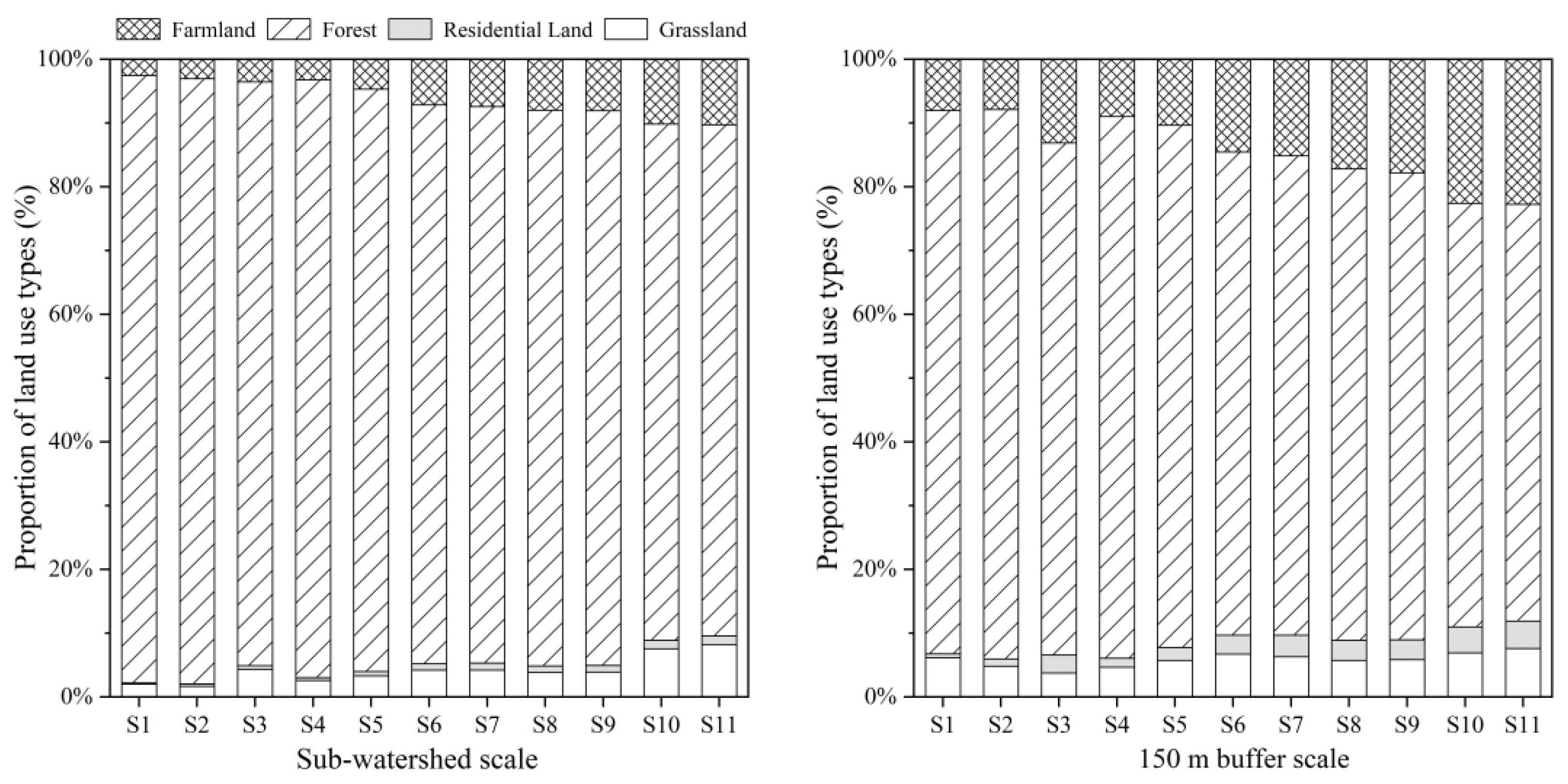
Forestland is the main land use type within the watershed (Figure 2). At the sub-watershed, the proportion of forestland ranges from 80.15% to 95.27% (averaging 88.82%), while grassland, residential land, and agricultural land account for smaller fractions, averaging 4.16%, 0.84%, and 6.18%, respectively. Within the 150 m buffer scales, the land use types are very similar to those of the sub-watershed, with forestland being the dominant type, accounting for more than 65.37%. Overall, the proportions of agricultural land, forestland, residential land, and grassland within the 150 m buffer scales are 14.38%, 2.64%, 77.13%, and 5.85%, respectively. In addition, at both the sub-watershed and 150 m buffer scales, the proportion of agricultural land generally increases from upstream to downstream, while the proportion of residential land shows the opposite trend.

Compared with the 150 m buffer scales, the AI and LSI are higher at the sub-watershed; while the ED, IJI, LPI, and PD are lower (

Table 4. Landscape index characteristics at different scales.

landscape Metrics	Unit	150 m Buffer Scale				Sub-Watershed Scale
		Min	Max	Avg	SD	Min	Max	Avg	SD
AIgra *	%	97.71	98.07	97.84	0.11	97.72	98.62	98.16	0.26
AIres		96.40	98.04	96.76	0.47	96.40	98.04	96.82	0.47
AIfor *		99.40	99.74	99.55	0.13	99.75	99.91	99.83	0.06
AIfar		98.48	99.23	98.71	0.22	98.55	99.24	98.75	0.20
EDgra *	m/ha	72.11	122.37	104.60	14.41	34.05	92.89	60.77	18.08
EDres *		13.96	108.93	74.66	31.91	4.38	36.44	23.50	10.83
EDfor *		148.70	266.24	223.94	47.24	49.30	151.61	109.80	35.91
EDfar *		62.03	212.87	157.28	55.25	19.97	97.69	67.11	30.26
IJIgra	%	25.79	77.85	56.54	16.30	14.36	60.78	45.77	16.44
IJIres		57.70	93.71	84.96	9.55	57.70	93.88	84.54	10.60
IJIfor		63.42	92.38	87.02	8.40	62.64	87.39	82.11	7.38
IJIfar		64.64	81.42	71.67	5.10	61.09	79.35	68.13	5.94
LPIgra	%	0.64	2.62	1.16	0.65	0.31	1.67	0.75	0.43
LPIres *		0.60	3.39	2.07	0.88	0.19	1.09	0.64	0.29
LPIfor *		13.78	84.98	42.21	27.75	65.58	95.20	86.29	9.73
LPIfar *		1.50	5.74	2.86	1.26	0.49	1.80	1.02	0.44
LSIgra	-	6.21	25.79	15.61	6.91	6.38	32.47	18.75	9.04
LSIres		2.67	28.88	16.56	9.16	2.67	29.50	16.55	9.75
LSIfor		3.66	22.45	12.65	6.96	2.66	18.17	9.55	5.52
LSIfar		3.37	25.14	15.45	8.23	3.36	29.57	17.50	10.16
PDgra *	n/km2	16.70	31.82	25.69	4.48	5.24	21.52	13.22	4.49
PDres*		10.02	19.65	15.37	3.91	3.15	7.55	5.33	1.77
PDfor *		11.82	32.23	22.72	7.41	2.75	9.22	5.84	2.10
PDfar *		15.78	40.25	31.25	9.59	5.24	15.46	11.42	4.19
PLANDgra *	%	3.76	7.60	5.85	1.10	1.66	8.16	4.16	2.04
PLANDres *		0.62	4.31	2.64	1.20	0.20	1.43	0.84	0.41
PLANDfor *		65.37	86.17	77.13	7.25	80.15	95.27	88.82	5.13
PLANDfar *		7.85	22.73	14.38	5.36	2.53	10.25	6.18	2.87

Notes: Aggregation Index (AI), Edge Density (ED), Interspersion and Juxtaposition Index (IJI), Largest Patch Index (LPI), Landscape Shape Index (LSI), Patch Density (PD), Percentage of Landscape (PLAND), Grassland (gra), Residential land (res), Forest (for), Farmland (far), Average (Avg), Standard deviation (SD). * indicates a significant difference in the landscape metrics between the Sub-watershed scale and 150 m buffer scale (p < 0.05).

). At both the sub-watershed and 150 m buffer scales, the AI, ED, and LPI are highest in the forest. The PD is highest in agricultural land at the 150 m buffer scales, while it is highest in grassland at the sub-watershed. The LSI and IJI are relatively higher in grassland (18.75) and residential land (84.54%) at the sub-watershed, respectively, while at the 150 m buffer scales, the LSI and IJI are higher in residential land (16.56) and forest (87.02%), respectively. Overall, the sub-watersheds are characterized by uniformly distributed and regularly shaped patches, indicating a highly concentrated landscape with low fragmentation. In contrast, the buffer zones consist mainly of single, large, and homogeneous patches, exhibiting a fragmented landscape distribution. The landscape pattern at the buffer zone scale demonstrates severe fragmentation and high dispersion.

3.2. Seasonal and Spatial Dynamics of Water Quality

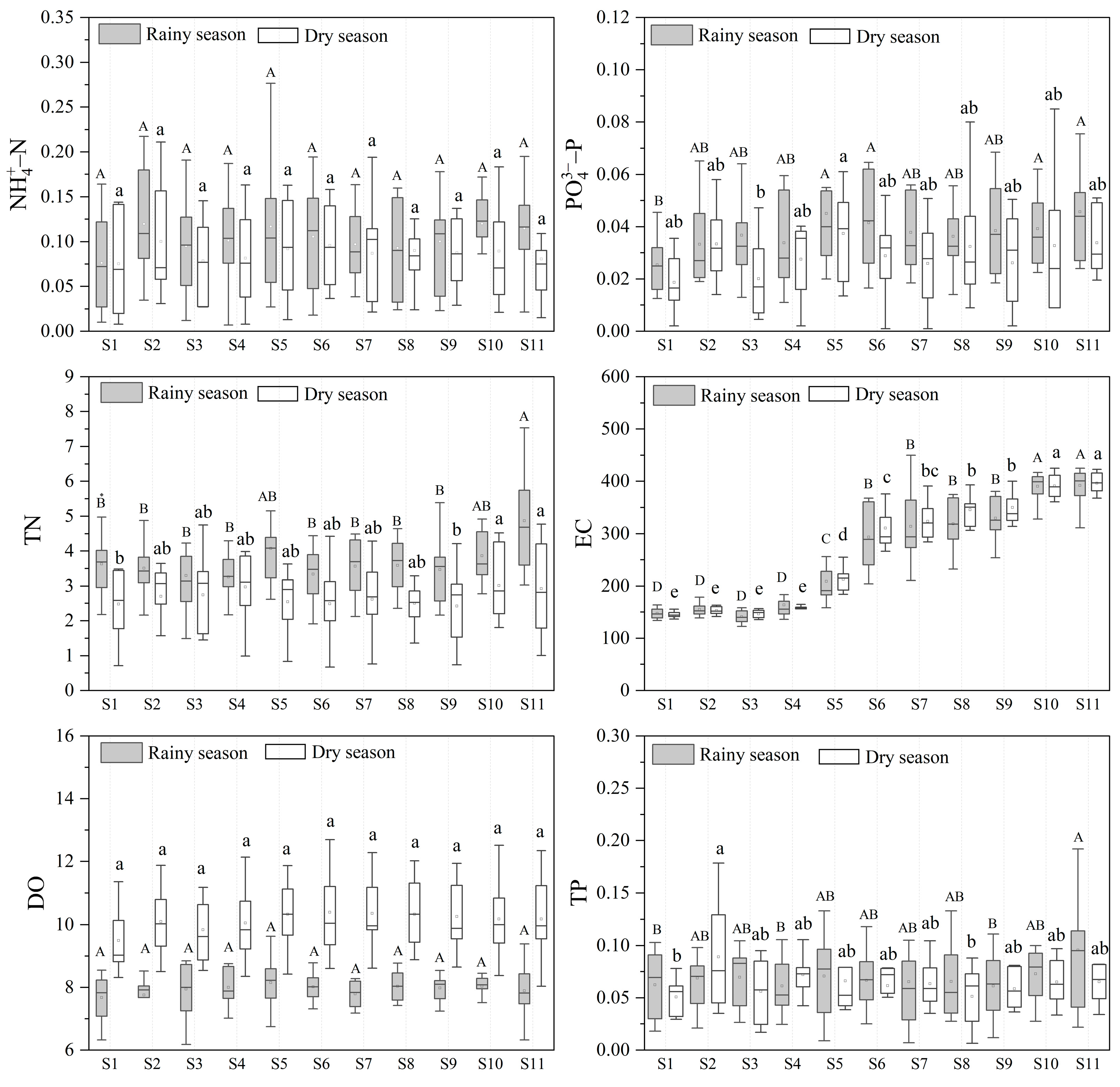
The temporal and spatial variations of water quality parameters across different seasons are illustrated in Figure 3. Significant seasonal differences were detected for all indicators, except for TP and electrical conductivity (EC) (p < 0.05). Concentrations of ammonia nitrogen, orthophosphate, and TN were found to be higher during the rainy season compared to the dry season, whereas EC and dissolved oxygen (DO) exhibited higher values in the dry season than in the rainy season. The average value of DO in the rainy season was 7.93 mg/L (which meets the Class I surface water quality standard; GB3838–2002 [50]), whereas in the dry season, DO was higher, at 10.14 mg/L (Class I). The mean concentration of TN during the rainy season (3.69 mg/L) was higher than that recorded in the dry season (2.66 mg/L) across all sampling sites, with the majority of sites exceeding the Class V water quality standard (2 mg/L). In contrast, the average concentration of TP was similar in the rainy season (0.069 mg/L) and the dry season (0.064 mg/L), both meeting the Class II water quality standard. The average concentrations of ammonia nitrogen in the rainy and dry seasons were 0.10 and 0.088 mg/L, respectively, both meeting the Class I water quality standard. EC increased from upstream to downstream, and its average value was lower in the rainy season (257.54 μS/cm) than in the dry season (268.20 μS/cm).

During the entire study period, no significant spatial variation trend was observed for TN and TP concentrations from upstream to downstream within the watershed. Significant differences in DO concentrations were observed across seasons (dry vs. rainy) (p < 0.05), with higher concentrations at sampling sites S5 to S9 during the rainy season and at sites S3 to S5 in the dry season. The spatial variation trends of ammonia nitrogen and orthophosphate concentrations were not significant, with the lowest concentrations observed at sampling site S1. Additionally, the highest concentration of ammonia nitrogen was observed at sampling site S2, while the highest concentration of orthophosphate was observed at sampling site S11. The spatial variation trend of EC was the most pronounced, with the lowest concentration observed at sampling site S1 and a continuous increase from site S1 to site S11, reaching the highest concentration at site S11.

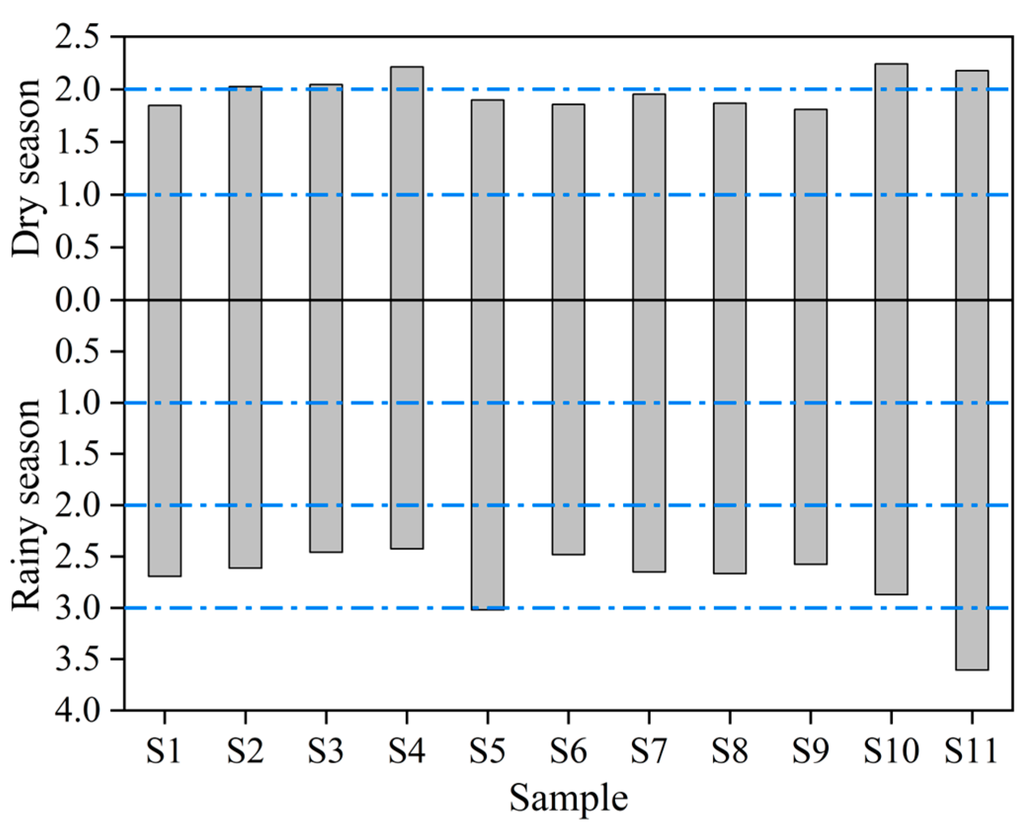
The evaluation results of the Nemerow Pollution Index for each indicator within the watershed are presented in Figure 4, with better water quality conditions observed in the dry season than in the rainy season. In the dry season, except for sampling sites S3, S4, S10, and S11, which were moderately polluted, the remaining sampling sites were mildly polluted. In the rainy season, except for sampling sites S5 and S11, which were severely polluted, the remaining sampling sites were moderately polluted. Combined with Figure 3, it can be seen that the water pollution is attributed to the high concentration of total nitrogen.

3.3. Influences of Landscape Pattern on Water Quality

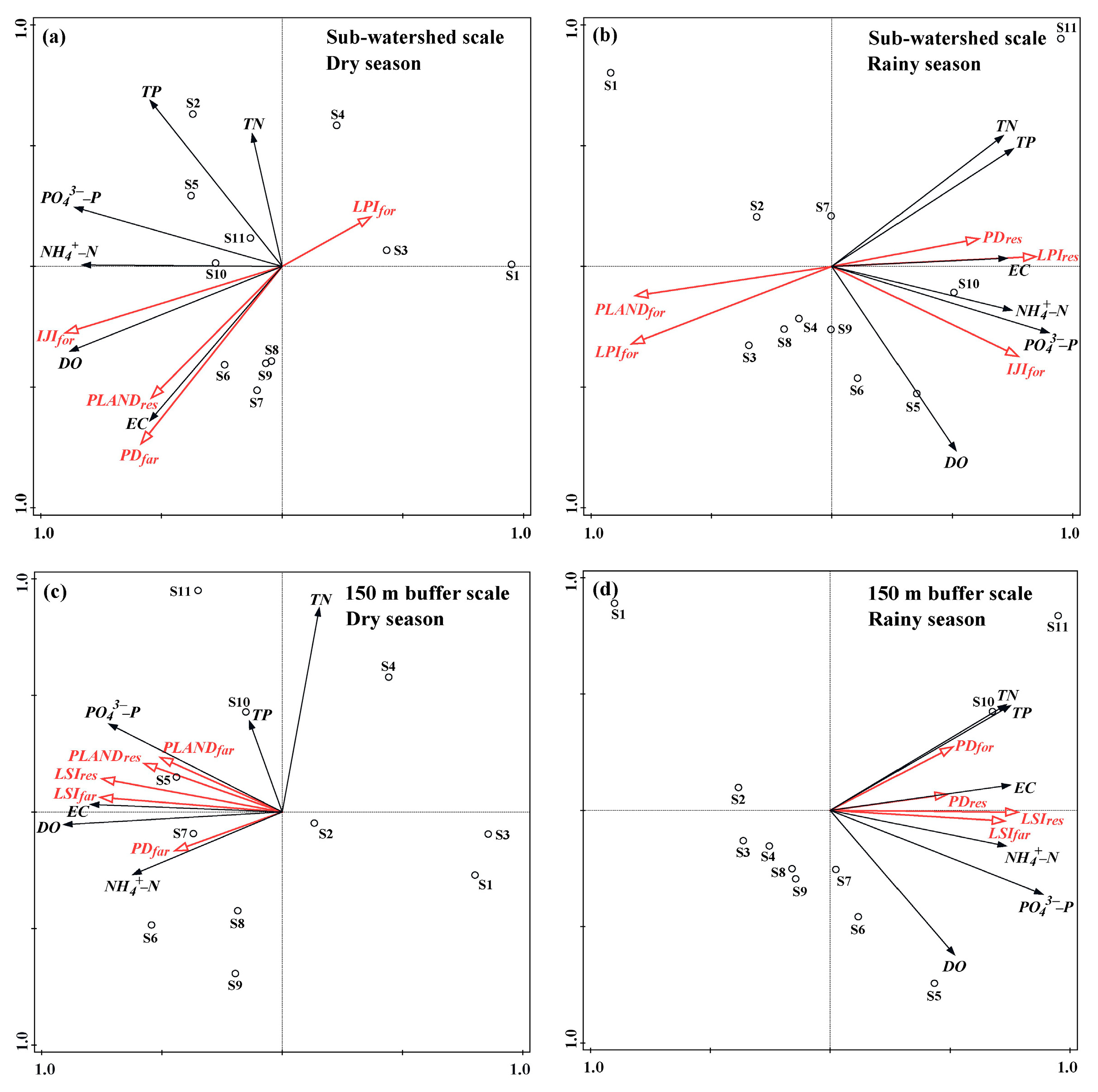
Results from the redundancy analysis (RDA) indicated that landscape pattern indices at both the sub-watershed and 150 m buffer scales accounted for over 76% of spatiotemporal water quality variations, with significant seasonal and spatial-scale differences (p < 0.05) (

Table 5. RDA explains the impact of landscape indicators on seasonal water quality at different spatial scales.

Scales	Season	Total Explanation	Explanatory Rate of Significant Landscape Metrics
Sub-watershed scale	Dry season	88.0%	IJIfor (40.7%), PDfar (19.2%), PLANDres (17.7%), LPIfor (10.3%)
	Rainy season	89.2%	LPIfor (40.1%), IJIfor (17.7%), PDres (15.1%), PLANDfor (9.3%), LPIres (7.1%)
150 m Buffer scale	Dry season	76.1%	LSIres (28.8%), PLANDfar (20.3%), LSIfar (15.2%), PDfar (4.9%), PLANDres (6.9%)
	Rainy season	85.9%	LSIres (36.8%), LSIfar (21.2%), PDfor (14.1%), PDres (8.7%)

and Figure 5). At the sub-watershed scale, the total explanations of landscape indicators for water quality changes reached 88.0% and 89.2% during dry and rainy seasons, respectively. In contrast to the sub-watershed scale, the total explanations of landscape indicators at the 150 m buffer scale decreased by 8.3–11.9%. At the sub-watershed scale, IJI_for, LPI_for, PD_far, PLAND_res, and PD_res were identified as key landscape drivers, exhibiting contributions of 17.7–40.7%, 10.3–40.1%, 19.2%, 17.7%, and 15.1%, respectively. At the 150 m buffer scale, LSI_res, LSI_far, PLAND_far, and PD_for demonstrated substantial explanatory contributions (28.8–36.8%, 15.2–21.2%, 20.3%, and 14.1%, respectively). The RDA ordination diagram revealed that IJI_for, PD_res, PLAND_res, PLAND_far, LPI_res, LSI_res, LSI_far, and PD_for exhibited positive correlations with most water quality parameters whereas PD_far showed negative correlations with TN and TP. Conversely, PLAND_for and LPI_for were negatively correlated with most parameters.

3.4. Threshold Analysis of Landscape Metrics Causing Abrupt Water Quality Changes

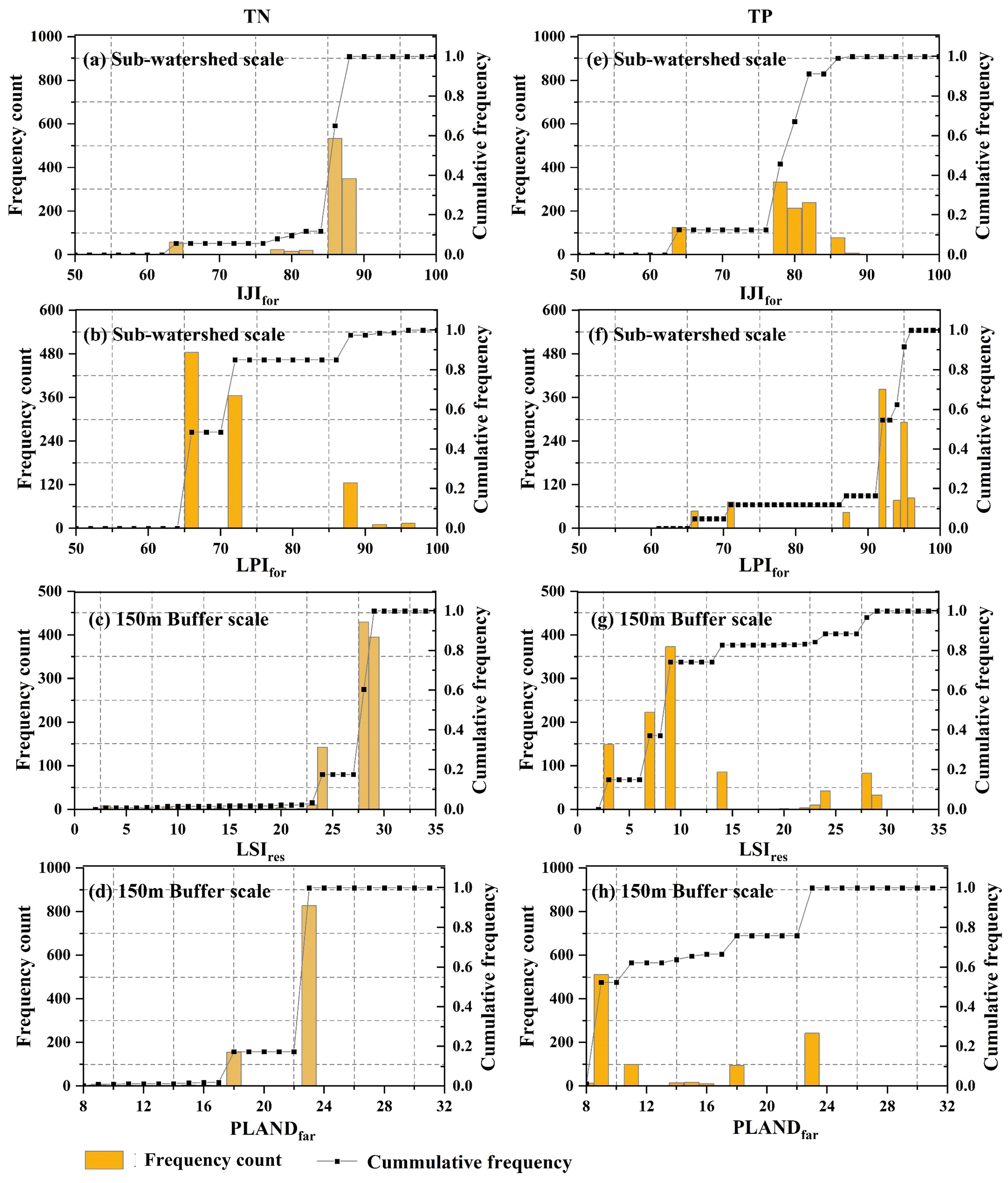
Based on the results of the RDA, the two most influential landscape metrics affecting TN and TP were identified at both the sub-watershed and buffer scales. The cumulative probabilities of abrupt changes in TN and TP along gradients of these metrics were then analyzed across different land use types (Figure 6). The smaller breakpoint value between the two scales (sub-watershed and buffer) was considered the threshold for each metric’s influence on TN and TP. For TN, at the sub-watershed level, the critical range for IJI_for was between 84% and 86%. When IJI_for exceeded 86%, the cumulative probability of abrupt change in TN increased to as high as 99.9%. Similarly, when LPI_for exceeded 70%, the cumulative probability of TN rose from 48.4% to 84.9%. At the 150 m buffer scale, the threshold for LSI_res was determined to be 27, with a corresponding change in the cumulative probability of 42.9% across this threshold. The critical range for PLAND_far was between 21% and 22%, beyond which the probability of abrupt TN changes increased dramatically from 17.3% to 99.9%.

The thresholds for TP were different from TN. At the sub-watershed scale, the threshold for LJI_for was 80%, which was 6% lower than TN. Across this threshold, the cumulative probability of abrupt TP change increased from 67.2% to 91.2%. The critical range for LPI_for was between 93% and 94%, when LPI_for exceeded 94%, the cumulative probability of TP reached 91.6%. At the 150 m buffer scale, both LSI_res and PLAND_far showed threshold values of 8. The cumulative probability of TP changed by 37.2% and 51.1%, respectively, across these thresholds. Overall, to reduce how landscape patterns affect water quality (TN and TP), the following thresholds are suggested as effective management targets: at the sub-watershed scale, LJI_for < 80% and LPI_for > 94%; at the 150 m buffer scale, LSI_res < 8 and PLAND_far < 8%.

4. Discussion

4.1. Influence Factors of Water Quality Variation

A significant correlation exists between water quality and landscape patterns, driven by the influence of landscape configuration on runoff dynamics, which spatially redistribute pollutants and nutrients by altering their transport pathways within river systems [8,51]. Regarding land use, the proportion of forest land (PLAND_for) exhibited negative correlations with TN and TP, aligning with findings by Liu et al. [52]. Forests act as critical sinks for nitrogen and phosphorus, effectively retaining these nutrients within catchments [53]. Consequently, increased PLAND_for can significantly reduce nutrient concentrations in riverine systems [52]. Although grassland was excluded from the RDA analysis due to multicollinearity with other landscape variables, this exclusion reflects statistical redundancy rather than the absence of ecological influence. Numerous studies have demonstrated that grassland, like forest, enhances water quality by reducing runoff, intercepting pollutants, and stabilizing soil, particularly at larger watershed scales [1,3,8,10,17,19]. Therefore, maintaining grasslands of a certain width and area within riparian buffer zones is important for the long-term water quality stability. Residential land (PLAND_res) and farmland (PLAND_far) proportions showed positive correlations with most water quality parameters, indicating that urbanization and agricultural expansion degrade river water quality patterns, consistent with prior studies [54,55]. Untreated domestic sewage and waste from human activities were often discharged directly into rivers due to inadequate centralized treatment infrastructure, exacerbating water quality degradation [56,57]. Agriculture has been well-documented as a major source contributing to nitrogen and phosphorus contamination of aquatic ecosystems [58,59]. Fertilizers and pesticides applied to farmland were transported into water bodies via surface runoff or subsurface drainage [60,61]. Excessive fertilization can also cause soil compaction, accelerating surface runoff convergence, and elevating soil erosion risks [19].

In landscape configuration, LPI_for exhibited negative correlations with most water quality parameters, while PD_far was inversely associated with TN and TP. Elevated LPI_for enhances catchment water quality by promoting nutrient retention [38,52], whereas fragmented farmland landscapes mitigate surface runoff pathways, reducing erosion, sediment transport, and subsequent nitrogen/phosphorus loads in runoff [59]. Furthermore, IJI_for, PD_for, PD_res, LPI_res, LSI_res, and LSI_far showed positive correlations with most parameters, suggesting that higher values of these indices correspond to greater water quality degradation. Increased forest patch fragmentation (PD_for) elevates runoff, while higher patch integrity (IJI_for) enhances nitrogen/phosphorus retention, exacerbating water quality deterioration [62,63]. Consistent with prior research [64], greater residential land fragmentation (PD_res) and human activity intensity were linked to pronounced water quality degradation. The Landscape Shape Index (LSI) quantifies patch shape complexity. Human activities, such as road construction and farmland division, increase LSI values for residential land and farmland by introducing irregular boundaries. This study demonstrated that complex patch shapes in residential and agricultural landscapes negatively influenced the quality of riverine water.

The RDA results revealed that the sub-watershed scale provides a stronger explanation for river water quality variations than the riparian buffer scale. This underscores that water quality management was inherently a regional issue, aligning with findings from prior studies [1,19]. Pollutant dynamics are predominantly driven by large-scale diffusion processes [20,59], which are more effectively captured at the sub-watershed scale than in small-scale riparian buffers. Furthermore, landscape pattern impacts on water quality exhibit distinct scale-dependent effects across land use types. Forest landscapes exert a stronger influence at broader spatial scales, whereas residential land and farmland demonstrate more pronounced effects at smaller scales. At the sub-watershed scale, forest landscape pattern indices explained 51.0–67.1% of water quality variations, accounting for over half of the total explained variance. This likely reflects the dominance of forest land (>80% coverage) as the primary land use within sub-watersheds. Conversely, the pollutant interception capacity of riparian forests may diminish due to their proximity to river channels, which can limit their buffering efficacy [65,66]. In contrast, at the riparian buffer scale, residential and agricultural landscape indices explained 35.5–45.5% and 21.2–35.5% of water quality variations, respectively, surpassing the contributions from forest land. This disparity may arise from elevated proportions of residential land (0.4–2.9%) and farmland (4.8–12.5%) within riparian buffers relative to sub-watersheds.

Cropland and residential land in the study area are mainly distributed along the riverbanks, and their proportions increasing along the upstream to downstream gradient. This riparian distribution pattern shortens the transport distance from pollution sources to the river, making pollutants generated by agricultural activities and domestic sources more likely to be transported into the river by runoff during rainfall events. In addition, the riparian-adjacent areas exhibit a relatively high degree of landscape fragmentation, which may enhance hydrological connectivity between surface runoff and the river channel, thereby increasing the efficiency of pollutant delivery to the river during rainfall events [67]. Under such conditions, the large amount of surface runoff generated during rainfall not only increases pollutant input fluxes but may also exceed the dilution effect of precipitation, ultimately resulting in elevated concentrations of N and P in the river during the wet season. DO serves as a key measure of ecosystem health in water bodies. In this study, DO concentrations were higher in the dry season than in the wet season, which is mainly attributed to seasonal temperature variations [1]. Elevated temperatures during the wet season can stimulate metabolic activity within microbial and aquatic communities, leading to increased oxygen consumption and decreased DO concentrations [68]. In addition, stronger runoff processes during the wet season may increase the input of organic matter and nutrients, further stimulating microbial oxygen consumption [67].

4.2. Key Landscape Threshold Intervals for Stream Risk Management

Landscape thresholds provide explicit ecological risk thresholds and actionable guidance for land use regulation in watershed management, thereby facilitating the development of scientifically informed spatial pattern optimization strategies aimed at protecting water quality and ecosystem functions. The findings underscore the necessity of regulating key landscape metrics at appropriate spatial scales to safeguard water health. Specifically, at the sub-watershed scale, LJI_for < 80% and LPI_for > 94% are recommended. At the 150 m riparian buffer scale, LSI_res < 8 and PLAND_far < 8%. The IJI quantifies the adjacency and intermixing of forest patches with other land use types. A high IJI (>80%) indicates that forest patches are finely interspersed with agricultural, urban, or barren lands. Under such conditions, the interface length between forest and non-forest patches is maximized. This extensive boundary zone facilitates the transfer of pollutants (e.g., fertilizers, livestock waste, eroded soil) from non-forest areas into the forested landscape and ultimately into the stream. More importantly, when LJI_for > 80%, forest patches become increasingly fragmented and spatially dispersed. This heightened landscape heterogeneity can result in greater nutrient losses [69]. Liu et al. [70] reported a higher IJI threshold (<92%) for maintaining water quality, which is higher than the threshold identified in this study. In steep mountainous terrains, excessive mixing of forest with high-risk land uses (e.g., cropland) enhances pollutant transport via slope runoff, accelerating degradation. The LPI reflects the area proportion of the dominant forest patch. When LPI_for is above 94%, the landscape is characterized by an almost continuous, well-connected forest matrix. In such a state, the forest provides optimal hydrological regulation and pollutant retention: rainfall is largely intercepted by canopy, runoff velocity is low, and most nutrients (TN, TP) and sediments are absorbed or filtered before reaching the stream. Once LPI_for drops below 94%, the dominant forest patch becomes fragmented, creating openings or corridors that connect upland non-forest areas (e.g., cropland, residential areas) to the stream network.

Riparian buffer zones, directly adjacent to water bodies, exhibit heightened sensitivity to pollutant interception and attenuation due to their landscape configuration [48,66]. Liu et al. [41] emphasized that water quality is more strongly affected at the riparian buffer scale. Numerous studies have demonstrated that the expansion of agricultural and urban land within these zones significantly degrades river water quality [71]. Minimizing LSI_res and PLAND_far can reduce the interface between residential areas and water bodies while limiting agricultural non-point source pollution. Xu et al. [67] reported that water quality was enhanced when LSI was below 18.5, our findings reveal a substantially lower threshold for LSI_res at the 150 m riparian buffer scale (LSI_res < 8). Despite the differences in spatial scale, both studies consistently indicate that lower landscape shape index reflect more regular and contiguous land-use boundaries, enhancing the ecological filtration capacity of riparian buffers by facilitating the interception of non-point source pollutants. The threshold for PLAND_far also varies across different buffer scales and regions. Qiu et al. [72] identified a 60% farmland coverage threshold in the Yahara watershed, whereas our study identified a substantially lower threshold of 8% for PLAND_far at the 150 m buffer scale. This discrepancy may result partly from regional differences in land use patterns and underlying surface conditions. Additionally, larger spatial scales often introduce greater landscape heterogeneity, which can attenuate the observable impact of farmland proportions. Farmland in close proximity to water bodies typically exhibits greater direct interaction with aquatic systems, characterized by shorter pollutant transport pathways and heightened sensitivity to land use changes.

Previous studies have demonstrated the existence of environmental thresholds associated with abrupt changes in water quality. Nevertheless, due to variations in land use, topography, watershed size, and other environmental factors, the specific types and ranges of these thresholds vary regionally [35,68,70,73]. Therefore, identifying multiscale landscape thresholds is critical for effective watershed management. Regarding forested areas, maintaining moderate landscape heterogeneity (LJI_for < 80%) is recommended to avoid excessive homogenization, while the protection and expansion of large forest patches (LPI_for > 94%) should be prioritized to enhance the mitigation of nitrogen and phosphorus pollution. For residential areas, minimizing boundary complexity (LSI_res < 8) is necessary to prevent unregulated expansion and mitigate direct disturbances to river systems. In agricultural management, strict control of farmland proportion within the 150 m buffer scale (PLAND_far < 8%) is necessary to reduce non-point source pollution and enhance the ecological functions of riparian buffers. These threshold-based strategies provide critical guidance for ecological conservation and water quality management in the Danjiangkou Reservoir source area. Future research should integrate multi-temporal datasets and modeling simulations to further validate the underlying mechanisms and regional applicability of landscape pattern thresholds.

5. Conclusions

Land use and landscape patterns significantly affected river water quality, with spa-tial scale and seasonal variations. Landscape indicators at the sub-watershed scale provided higher cumulative explanations for water quality variations than those at the 150 m buffer scale, and their relationship with water quality was stronger during the rainy season compared to the dry season. LPI_for, IJI_for, LSI_res, and PLAND_far are the most important landscape indicators influencing changes in water quality. Changes along the gradient of key landscape metrics cause a very high probability of abrupt water quality changes. Stream water quality degradation will be significantly accelerated when LPI is below 94% and IJI is above 80% for forested land at the sub-watershed scale, and when LSI is above 8 for residential land and the proportion of farmland land exceeds 8%t at the 150 m buffer scale. In watershed landscape planning and water resource management, maintaining sufficient areas of forest and grassland at the watershed scale especially around water bodies is important. In addition, considering threshold intervals for key landscape indicators in watershed landscape planning and water resource management is vital to reduce the risk of water quality degradation. To prevent water quality deterioration in the watershed, similar areas in the water source region may adopt these thresholds as indicators for landscape planning. These measures aid in curbing non-point source pollution and boosting water conservation capacity.

References

1. Xu, G.C.; Li, P.; Lu, K.X.; Zhang, T.T.; Zhang, J.X.; Ren, Z.P.; Wang, X.K.; Yu, K.X.; Shi, P.; Cheng, Y.T. Seasonal changes in water quality and its main influencing factors in the Dan River basin. Catena 2019, 173, 131–140. [Google Scholar] [CrossRef]
2. Wijesiri, B.; Deilami, K.; McGree, J.; Goonetilleke, A. Use of surrogate indicators for the evaluation of potential health risks due to poor urban water quality: A Bayesian Network approach. Environ. Pollut. 2018, 233, 655–661. [Google Scholar] [CrossRef] [PubMed]
3. Sun, X.W.; Zhang, H.Y.; Zhong, M.F.; Wang, Z.Y.; Liang, X.Q.; Huang, T.S.; Huang, H. Analyses on the temporal and spatial characteristics of water quality in a seagoing river using multivariate statistical techniques: A case study in the Duliujian River, China. Int. J. Environ. Res. Public Health 2019, 16, 1020. [Google Scholar] [CrossRef] [PubMed]
4. Xu, H.X.; Gao, Q.; Yuan, B. Analysis and identification of pollution sources of comprehensive river water quality: Evidence from two river basins in China. Ecol. Indic. 2022, 135, 108561. [Google Scholar] [CrossRef]
5. Bracken, L.J.; Wainwright, J.; Ali, G.A.; Tetzlaff, D.; Smith, M.W.; Reaney, S.M.; Roy, A.G. Concepts of hydrological connectivity: Research approaches, pathways and future agendas. Earth-Sci. Rev. 2013, 119, 17–34. [Google Scholar] [CrossRef]
6. Krupa, M.; Tate, K.W.; van Kessel, C.; Sarwar, N.; Linquist, B.A. Water quality in rice-growing watersheds in a Mediterranean climate. Agric. Ecosyst. Environ. 2011, 144, 290–301. [Google Scholar] [CrossRef]
7. Orwin, J.F.; Klotz, F.; Taube, N.; Kerr, J.G.; Laceby, J.P. Linking catchment structural units (CSUs) with water quality: Implications for ambient monitoring network design and data interpretation. J. Environ. Manag. 2022, 312, 114881. [Google Scholar] [CrossRef] [PubMed]
8. Cheng, X.; Song, J.P.; Yan, J.Z. Influences of landscape pattern on water quality at multiple scales in an agricultural basin of western China. Environ. Pollut. 2023, 319, 120986. [Google Scholar] [CrossRef]
9. Mouri, G.; Takizawa, S.; Oki, T. Spatial and temporal variation in nutrient parameters in stream water in a rural-urban catchment, Shikoku, Japan: Effects of land cover and human impact. J. Environ. Manag. 2011, 92, 1837–1848. [Google Scholar] [CrossRef]
10. Wu, L.; Long, T.Y.; Liu, X.; Guo, J.S. Impacts of climate and land-use changes on the migration of non-point source nitrogen and phosphorus during rainfall-runoff in the Jialing River Watershed, China. J. Hydrol. 2012, 475, 26–41. [Google Scholar] [CrossRef]
11. Shrestha, S.; Bhatta, B.; Shrestha, M.; Shrestha, P.K. Integrated assessment of the climate and landuse change impact on hydrology and water quality in the Songkhram River Basin, Thailand. Sci. Total Environ. 2018, 643, 1610–1622. [Google Scholar] [CrossRef] [PubMed]
12. Wang, R.; Liu, L.; Tao, Z.; Wan, B.; Wang, Y.; Tang, X.; Li, Y.; Li, X. Effect of urbanization and urban forests on water quality improvement in the Yangtze River Delta: A case study in Hangzhou, China. J. Environ. Manag. 2024, 351, 119980. [Google Scholar] [CrossRef]
13. Mehdi, B.; Ludwig, R.; Lehner, B. Evaluating the impacts of climate change and crop land use change on streamflow, nitrates and phosphorus: A modeling study in Bavaria. J. Hydrol. Reg. Stud. 2015, 4, 60–90. [Google Scholar] [CrossRef]
14. Moreno-Mateos, D.; Mander, Ü.; Comín, F.A.; Pedrocchi, C.; Uuemaa, E. Relationships between landscape pattern, wetland characteristics, and water quality in agricultural catchments. J. Environ. Qual. 2008, 37, 2170–2180. [Google Scholar] [CrossRef]
15. Alexakis, D.D.; Grillakis, M.G.; Koutroulis, A.G.; Agapiou, A.; Themistocleous, K.; Tsanis, I.K.; Retalis, A.; Tymvios, F.; Hadjimitsis, D.G. GIS and remote sensing techniques for the assessment of land use change impact on flood hydrology: The case study of Yialias basin in Cyprus. Nat. Hazards Earth Syst. Sci. 2014, 14, 413–426. [Google Scholar] [CrossRef]
16. Liu, T.; Yang, X.J. Monitoring land changes in an urban area using satellite imagery, GIS and landscape metrics. Appl. Geogr. 2015, 56, 42–54. [Google Scholar] [CrossRef]
17. Shi, P.; Zhang, Y.; Li, Z.B.; Li, P.; Xu, G.C. Influence of land use and land cover patterns on seasonal water quality at multi-spatial scales. Catena 2017, 151, 182–190. [Google Scholar] [CrossRef]
18. Zhang, F.; Chen, Y.; Wang, W.W.; Jim, C.Y.; Zhang, Z.M.; Tan, M.L.; Liu, C.J.; Chan, N.W.; Wang, D.; Wang, Z.; et al. Impact of land-use/land-cover and landscape pattern on seasonal in-stream water quality in small watersheds. J. Clean. Prod. 2022, 357, 131907. [Google Scholar] [CrossRef]
19. Zhang, S.; Yan, X.; Feng, T.; Zhang, X.; Qiao, R.X.; Ren, Y.F.; Chen, Q.F. Unraveling nonlinear impacts of land use change on riverine water quality under future scenarios. Ecol. Indic. 2025, 179, 114258. [Google Scholar] [CrossRef]
20. Li, J.; Xi, H.H.; Wang, F.; Ding, X.; Chen, X.F.; Tao, Y.; Huang, C.H.; Tao, Q.; Cheng, X.B.; Ou, W.X. Non-linear responses of ecosystem service trade-offs to landscape heterogeneity: Implications for spatially targeted landscape management in an urbanizing agricultural basin. Landsc. Urban Plan. 2026, 271, 105642. [Google Scholar] [CrossRef]
21. Han, Y.Y.; Zhang, K.; Lin, Q.; Huang, S.X.; Yang, X.D. Assessing lake ecosystem health from disturbed anthropogenic landscapes: Spatial patterns and driving mechanisms. Ecol. Indic. 2023, 147, 110007. [Google Scholar] [CrossRef]
22. Wang, Y.C.; Wu, H.W.; Pan, Z.Q.; Ma, L.D.; Zhang, Y.; Zhou, J.; Hu, M.P.; Cheng, Z.H.; Zheng, X.; Chen, D.J. Influence of land use and landscape pattern on legacy nitrogen pollution in a typical watershed in eastern China. Catena 2025, 256, 109129. [Google Scholar] [CrossRef]
23. Han, H.J.; Yan, X.; Li, X.R.; Yang, X.; Li, X.H.; Huang, Z.L.; Yan, X.Y.; Xia, Y.Q. Prioritizing riparian scale landscape management is a spatially efficient strategy for controlling river water quality in China. Water Res. 2026, 301, 126002. [Google Scholar] [CrossRef] [PubMed]
24. Xu, M.Z.; Xu, G.C.; Li, Z.B.; Dang, Y.T.; Li, Q.S.; Min, Z.Q.; Gu, F.Y.; Wang, B.; Liu, S.B.; Zhang, Y.X. Effects of comprehensive landscape patterns on water quality and identification of key metrics thresholds causing its abrupt changes. Environ. Pollut. 2023, 333, 122097. [Google Scholar] [CrossRef]
25. Su, S.L.; Ma, K.; Zhou, T.H.; Yao, Y.T.; Xin, H.J. Advancing methodologies for assessing the impact of land use changes on water quality: A comprehensive review and recommendations. Environ. Geochem. Health 2025, 47, 101. [Google Scholar] [CrossRef]
26. Liu, S.C.; Ryu, D.; Webb, J.A.; Lintern, A.; Guo, D.L.; Waters, D.; Western, A.W. A Bayesian approach to understanding the key factors influencing temporal variability in stream water quality–a case study in the Great Barrier Reef catchments. Hydrol. Earth Syst. Sci. 2021, 25, 2663–2683. [Google Scholar] [CrossRef]
27. Cushman, S.A.; Wasserman, T.N. Landscape applications of machine learning: Comparing random forests and logistic regression in multi-scale optimized predictive modeling of American marten occurrence in northern Idaho, USA. In Machine Learning for Ecology and Sustainable Natural Resource Management; Springer: Berlin/Heidelberg, Germany, 2018; pp. 185–203. [Google Scholar] [CrossRef]
28. Ma, X.B.; Zhang, J.H.; Wang, P.J.; Zhou, L.Y.; Sun, Y. Estimating the nonlinear response of landscape patterns to ecological resilience using a random forest algorithm: Evidence from the Yangtze River Delta. Ecol. Indic. 2023, 153, 110409. [Google Scholar] [CrossRef]
29. Du, J.F.; Xiao, X.L.; Lin, D.; Zhang, G.L.; Li, H.Y.; Lei, Y.M.; Liu, J.C.; Lu, H.L.; Li, Y.; Hong, H.L. Deciphering Multi-Scale Anthropogenic Drivers of River Water Quality: A Synergistic ML-GAM Cascade Framework with Sentinel-2. Remote Sens. 2026, 18, 840. [Google Scholar] [CrossRef]
30. Murphy, R.R.; Perry, E.; Harcum, J.; Keisman, J. A generalized additive model approach to evaluating water quality: Chesapeake Bay case study. Environ. Model. Softw. 2019, 118, 1–13. [Google Scholar] [CrossRef]
31. King, R.S.; Richardson, C.J. Integrating bioassessment and ecological risk assessment: An approach to developing numerical water-quality criteria. Environ. Manag. 2003, 31, 795–809. [Google Scholar] [CrossRef]
32. Li, B.; Huang, X.L.; Zhong, Q.; Wu, X.X. Impact of forest fragmentation on river water quality: An example from a typical subtropical hilly basin. PeerJ 2025, 13, e19435. [Google Scholar] [CrossRef] [PubMed]
33. Li, Y.; Boswell, E.; Thompson, A. Correlations between land use and stream nitrate-nitrite concentrations in the Yahara River Watershed in south-central Wisconsin. J. Environ. Manag. 2021, 278, 111535. [Google Scholar] [CrossRef]
34. Xu, Q.Y.; Yan, T.Z.; Wang, C.Y.; Hua, L.L.; Zhai, L.M. Managing landscape patterns at the riparian zone and sub-basin scale is equally important for water quality protection. Water Res. 2023, 229, 119280. [Google Scholar] [CrossRef]
35. Wu, J.H.; Lu, J. Landscape patterns regulate non-point source nutrient pollution in an agricultural watershed. Sci. Total Environ. 2019, 669, 377–388. [Google Scholar] [CrossRef]
36. Wu, J.H.; Lu, J. Spatial scale effects of landscape metrics on stream water quality and their seasonal changes. Water Res. 2021, 191, 116811. [Google Scholar] [CrossRef] [PubMed]
37. Clément, F.; Ruiz, J.; Rodríguez, M.A.; Blais, D.; Campeau, S. Landscape diversity and forest edge density regulate stream water quality in agricultural catchments. Ecol. Indic. 2017, 72, 627–639. [Google Scholar] [CrossRef]
38. Shen, Z.Y.; Hou, X.S.; Li, W.; Aini, G.Z.; Chen, L.; Gong, Y.W. Impact of landscape pattern at multiple spatial scales on water quality: A case study in a typical urbanised watershed in China. Ecol. Indic. 2015, 48, 417–427. [Google Scholar] [CrossRef]
39. King, R.S.; Baker, M.E. Considerations for analyzing ecological community thresholds in response to anthropogenic environmental gradients. J. N. Am. Benthol. Soc. 2010, 29, 998–1008. [Google Scholar] [CrossRef]
40. Huo, S.L.; Ma, C.Z.; Xi, B.D.; He, Z.F.; Su, J.; Wu, F.C. Nonparametric approaches for estimating regional lake nutrient thresholds. Ecol. Indic. 2015, 58, 225–234. [Google Scholar] [CrossRef]
41. Liu, X.; Shen, Y.J.; Chang, Y.R.; Shen, Y.J. The spatial scale and threshold effects of the relationship between landscape metrics and water quality in the Hutuo River Basin. J. Environ. Manag. 2024, 372, 123361. [Google Scholar] [CrossRef] [PubMed]
42. Wang, H.; Xiong, Q.Q.; Feng, Q.Y.; Xiao, S.Z.; Mu, D.J.; Sun, X.X.; Wang, S.J. Prediction and impact of Location-Weighted landscape Index on water quality in a typical karst region in southwest China: A case study of the Huanghou basin. Ecol. Indic. 2024, 165, 112186. [Google Scholar] [CrossRef]
43. Wang, S.D.; Liu, Y.Y.; Guo, J.H.; Liu, J.P.; Chai, H.B. Impacts of the Middle Route of the South-to-North Water Diversion Project on Land Surface Temperature and Fractional Vegetation Coverage in the Danjiang River Basin. Remote Sens. 2024, 16, 2665. [Google Scholar] [CrossRef]
44. Li, M.Y.; Liang, D.; Xia, J.; Song, J.X.; Cheng, D.D.; Wu, J.T.; Cao, Y.L.; Sun, H.T.; Li, Q. Evaluation of water conservation function of Danjiang River Basin in Qinling Mountains, China based on InVEST model. J. Environ. Manag. 2021, 286, 112212. [Google Scholar] [CrossRef]
45. Yu, S.; Xu, Z.; Wu, W.; Zuo, D. Effect of land use types on stream water quality under seasonal variation and topographic characteristics in the Wei River basin, China. Ecol. Indic. 2016, 60, 202–212. [Google Scholar] [CrossRef]
46. Zhao, M.; Zeng, C.; Liu, Z.; Wang, S. Effect of different land use/land cover on karst hydrogeochemistry: A paired catchment study of Chenqi and Dengzhanhe, Puding, Guizhou, SW China. J. Hydrol. 2010, 388, 121–130. [Google Scholar] [CrossRef]
47. Fang, S.; Gertner, G.; Wang, G.; Anderson, A. The Impact of Misclassification in Land Use Maps in the Prediction of Landscape Dynamics. Landsc. Ecol. 2006, 21, 233–242. [Google Scholar] [CrossRef]
48. Ariyan, T.N.; Quraishi, S.B.; Alam, M.N.E.; Khan, M.S.R.; Faria, F.F.; Kabir, A. Comprehensive analysis and human health risk assessment of tap water quality in Dhaka city, Bangladesh: Integrating source identification, index-based evaluation, and heavy metal assessment. J. Hazard. Mater. 2025, 5, 485. [Google Scholar] [CrossRef] [PubMed]
49. Qian, S.S.; King, R.S.; Richardson, C.J. Two statistical methods for the detection of environmental thresholds. Ecol. Model. 2003, 166, 87–97. [Google Scholar] [CrossRef]
50. GB3838–2002; Environmental Quality Standards for Surface Water. State Environmental Protection Administration, China: Beijing, China, 2002.
51. Shehab, Z.N.; Jamil, N.R.; Airs, A.Z.; Shafie, N.S. Spatial variation impact of landscape patterns and land use on water quality across an urbanized watershed in Bentong, Malaysia. Ecol. Indic. 2021, 122, 107254. [Google Scholar] [CrossRef]
52. Liu, J.; Liu, X.L.; Wang, Y.; Li, Y.; Jiang, Y.X.; Wang, M.H.; Wu, J.S. Landscape pattern at the class level regulates the stream water nitrogen and phosphorus levels in a Chinese subtropical agricultural catchment. Agric. Ecosyst. Environ. 2020, 295, 106897. [Google Scholar] [CrossRef]
53. Shen, Z.Y.; Chen, L.; Hong, Q.; Qiu, J.L.; Xie, H.; Liu, R.M. Assessment of nitrogen and phosphorus loads and causal factors from different land use and soil types in the Three Gorges Reservoir Area. Sci. Total Environ. 2013, 454–455, 383–392. [Google Scholar] [CrossRef] [PubMed]
54. Ou, Y.; Wang, X.Y.; Wang, L.X.; Rousseau, A.N. Landscape influences on water quality in riparian buffer zone of drinking water source area, Northern China. Environ. Earth Sci. 2016, 75, 114. [Google Scholar] [CrossRef]
55. Namugize, J.N.; Jewitt, G.; Graham, M. Effects of land use and land cover changes on water quality in the uMngeni river catchment, South Africa. Phys. Chem. Earth Parts A/B/C 2018, 105, 247–264. [Google Scholar] [CrossRef]
56. Wang, P.; Liu, J.Z.; Qi, S.H.; Wang, S.Q.; Chen, X.L. Tracing sources of nitrate using water chemistry, land use and nitrogen isotopes in the Ganjiang River, China. Isot. Environ. Health Stud. 2017, 53, 539–551. [Google Scholar] [CrossRef]
57. Hao, Z.; Zhang, X.Y.; Gao, Y.; Xu, Z.W.; Yang, F.T.; Wen, X.F.; Wang, Y.M. Nitrogen source track and associated isotopic dynamic characteristic in a complex ecosystem: A case study of a subtropical watershed, China. Environ. Pollut. 2018, 236, 77–187. [Google Scholar] [CrossRef] [PubMed]
58. Pérez-Gutiérrez, J.D.; Paz, J.O.; Tagert, M.L.M. Seasonal water quality changes in on-farm water storage systems in a south-central U.S. agricultural watershed. Agric. Water Manag. 2017, 187, 131–139. [Google Scholar] [CrossRef]
59. Lei, C.G.; Wagner, P.D.; Fohrer, N. Effects of land cover, topography, and soil on stream water quality at multiple spatial and seasonal scales in a German lowland catchment. Ecol. Indic. 2021, 120, 106940. [Google Scholar] [CrossRef]
60. Zhang, Y.; Li, F.D.; Zhang, Q.Y.; Li, J.; Liu, Q. Tracing nitrate pollution sources and transformation in surface- and ground-waters using environmental isotopes. Sci. Total Environ. 2014, 490, 213–222. [Google Scholar] [CrossRef] [PubMed]
61. Tanaka, M.O.; de Souza, A.L.T.; Moschini, L.E.; de Oliveira, A.K. Influence of watershed land use and riparian characteristics on biological indicators of stream water quality in southeastern Brazil. Agric. Ecosyst. Environ. 2016, 216, 333–339. [Google Scholar] [CrossRef]
62. Udawatta, R.P.; Henderson, G.S.; Jones, J.R.; Hammer, D. Phosphorus and nitrogen losses in relation to forest, pasture and row-crop land use and precipitation distribution in the midwest USA. J. Water Sci. 2011, 24, 269–281. [Google Scholar] [CrossRef]
63. Billmire, M.; Koziol, B.W. Landscape and flow path-based nutrient loading metrics for evaluation of in-stream water quality in Saginaw Bay, Michigan. J. Great Lakes Res. 2018, 44, 1068–1080. [Google Scholar] [CrossRef]
64. Li, K.; Chi, G.Q.; Wang, L.; Xie, Y.J.; Wang, X.R.; Fan, Z.Q. Identifying the critical riparian buffer zone with the strongest linkage between landscape characteristics and surface water quality. Ecol. Indic. 2018, 93, 741–752. [Google Scholar] [CrossRef]
65. Wang, W.; Wu, X.H.; Yin, C.M.; Xie, X.L. Nutrition loss through surface runoff from slope lands and its implications for agricultural management. Agric. Water Manag. 2019, 212, 226–231. [Google Scholar] [CrossRef]
66. Gu, Y.; Zhang, P.; Qin, F.; Cai, Y.; Li, C.; Wang, X. Enhancing river water quality in different seasons through management of landscape patterns at various spatial scales. J. Environ. Manag. 2025, 373, 123653. [Google Scholar] [CrossRef]
67. Xu, Y.; Li, P.; Ma, F.; Liu, X.; Zhang, N.; Pan, J.; Meng, Y. Watershed landscape characteristics and connectivity drive river water quality under seasonal dynamics. J. Clean. Prod. 2024, 473, 143533. [Google Scholar] [CrossRef]
68. Mei, K.; Shi, H.N.; Wu, Y.P.; Dahlgren, R.A.; Ji, X.L.; Yang, M.M.; Guan, Y.R. Impact of landscape patterns on river water quality: Spatial-scale effects across an agricultural-urban interface. Ecol. Indic. 2025, 170, 113019. [Google Scholar] [CrossRef]
69. Pak, H.Y.; Chuah, C.J.; Yong, E.L.; Snyder, S.A. Effects of land use configuration, seasonality and point source on water quality in a tropical watershed: A case study of the Johor River Basin. Sci. Total Environ. 2021, 780, 146661. [Google Scholar] [CrossRef] [PubMed]
70. Liu, H.; Meng, C.; Wang, Y.; Liu, X.; Li, Y.; Li, Y.; Wu, J. Multi-spatial scale effects of multidimensional landscape pattern on stream water nitrogen pollution in a subtropical agricultural watershed. J. Environ. Manag. 2022, 321, 115962. [Google Scholar] [CrossRef]
71. Tan, S.; Zhao, G.; Peng, C.; Ye, W.; Xie, D.; Chen, F.; Ni, C.; Shao, J.; Zheng, L.; Ni, J. Multi-scale effects of landscape on nitrogen (N) and phosphorus (P) in a subtropical agricultural watershed: A case of Qi river basin (QRB), China. Ecol. Indic. 2023, 147, 110017. [Google Scholar] [CrossRef]
72. Qiu, J.; Turner, M.G. Importance of landscape heterogeneity in sustaining hydrologic ecosystem services in an agricultural watershed. Ecosphere 2025, 6, art229. [Google Scholar] [CrossRef]
73. Wu, J.; Yang, Z.; Wang, H.; Xu, J. Scale effects and threshold management in the influence of landscape patterns on non-point source pollution. Ecol. Indic. 2025, 173, 113439. [Google Scholar] [CrossRef]
Figure 1. Schematic diagram of the study area location and sampling points. S1–S11 are the sampling sites, hereafter the same.
Sustainability 18 05426 g001
Figure 2. Proportion of land use at the sub-watershed and 150 m buffer scales.
Sustainability 18 05426 g002
Figure 3. Water quality parameters at 11 monitoring sites: spatiotemporal patterns. Rainy season: number = 495 (15 sampling campaigns × 11 sites × 3 replicates); Dry season: number = 330 (10 sampling campaigns × 11 sites × 3 replicates). Capital and lowercase letters denote statistically significant spatial variations in water quality during the rainy and dry seasons, respectively, at the 0.05 level. The white square in the box plot represent the average value.
Sustainability 18 05426 g003
Figure 4. Water quality assessment results of 11 monitoring points in different seasons. Ip ≤ 1 indicates no pollution; 1 < Ip ≤ 2 indicates slight pollution; 2 < Ip ≤ 3 indicates moderate pollution; 3 < Ip ≤ 5 indicates severe pollution.
Sustainability 18 05426 g004
Figure 5. RDA illustrating the relationship between water quality parameters (black line) and landscape indicators (red line) across seasonal and spatial scales. (a) Sub-watershed scale during dry season; (b) Sub-watershed scale during rainy season; (c) 150 m buffer scale during dry season; (d) 150 m buffer scale during rainy season.
Sustainability 18 05426 g005
Figure 6. The frequency distributions and cumulative curves of landscape metrics reflected water quality parameter abrupt change thresholds across different spatial scales.
Sustainability 18 05426 g006