Does Environmental Governance Specialization Reduce Air Pollution? Evidence from a Staggered Difference-in-Differences Approach in China

Abstract

Establishing specialized environmental adjudication divisions within China’s intermediate courts reduces local air pollution by approximately 3.9%. We examine this governance innovation using satellite-derived PM_2.5 data for 324 prefecture-level cities (2011–2023) and heterogeneity-robust difference-in-differences methods that address biases in conventional estimators under staggered treatment adoption. Under city-level clustering, which reflects the unit of treatment assignment, four complementary estimators (Callaway–Sant’Anna, Sun–Abraham, Borusyak–Jaravel–Spiess, and two-way fixed effects) consistently yield negative and statistically significant treatment effects (ATT ranging from $-0.037$ to $-0.054$, $p<0.05$). With the more conservative province-level clustering (31 clusters), significance attenuates for all estimators, with p-values ranging from 0.078 to 0.289; we interpret this as reflecting the small number of clusters rather than the absence of a true effect, although sensitivity to the clustering level remains a limitation. Event study analysis confirms parallel pre-treatment trends and persistent post-treatment effects. Heterogeneity patterns are directionally consistent but statistically inconclusive ($n=12$ cohorts): reductions appear larger in more industrialized and more polluted cohorts, though the precise mechanism remains unidentified. A spatial analysis finds no evidence of pollution displacement, but SUTVA is violated by concurrent court adoption in neighboring cities; once the neighbor pool is restricted to never-treated cities, the apparent negative spillover attenuates to non-significance, so the direction of bias in our main estimates cannot be determined. These results demonstrate that governance specialization can meaningfully complement regulatory instruments in advancing sustainability goals for air quality.

1. Introduction

China’s PM_2.5 concentrations have declined markedly since 2013, driven largely by command-and-control regulation under the Action Plan on Prevention and Control of Air Pollution [1]. Yet sustaining these gains, and achieving the targets embedded in Sustainable Development Goals 11 and 13, requires institutional mechanisms that go beyond top-down mandates [2]. More broadly, the literature on sustainability transitions emphasizes that durable environmental improvement depends not only on regulatory stringency but also on building effective, accountable, and inclusive institutions at all levels, the core aspiration of SDG Target 16.6 [3]. Whether specific governance innovations actually contribute to pollution reduction, or merely add administrative layers, is an empirical question that has received surprisingly little rigorous attention.

One such innovation is the establishment of specialized Environmental and Resource Adjudication Divisions within China’s intermediate courts. These divisions consolidate environmental cases, such as pollution damage claims, public interest litigation, and regulatory enforcement reviews, that were previously scattered across generalist divisions. Guiyang created the first such division in 2007; after a 2014 national directive, adoption accelerated, and by 2023 more than half of China’s prefecture-level cities had established such specialized divisions. Because cities adopted at different times (17 cohorts spanning 2007 to 2023, of which 12 fall within our analysis window of 2012–2023), the staggered rollout creates a natural experiment for estimating causal effects.

Why might governance specialization matter for pollution? Concentrated expertise may improve adjudication quality [4]; a dedicated division signals commitment to environmental protection and deters would-be polluters [5]; and specialization facilitates environmental public interest litigation (EPIL), opening new avenues for sanctioning violations [6,7]. Our empirical design directly tests the EPIL and administrative-penalty channels, while the deterrence channel, which operates through firm-level anticipation rather than observable state action, is examined only indirectly through cohort heterogeneity. Despite these plausible mechanisms, credible evidence that the reform actually reduces pollution is lacking, for two reasons.

The methodological reason is that existing studies rely on two-way fixed effect (TWFE) regression. Recent econometric work has shown that TWFE can produce biased, even sign-reversed, estimates when treatment effects vary across cohorts [8,9,10,11]. With 17 adoption cohorts spanning 2007 to 2023 (12 of which fall within our analysis window), this bias is a concrete threat here, not an abstract concern.

The data-related reason is that prior studies measure pollution using government statistical yearbooks, which local officials may manipulate [2,12]. Wu et al. [6] explicitly identify this problem, calling for objective measures in future research.

We address both issues. Our outcome variable is satellite-derived PM_2.5 concentration, immune to local manipulation. For causal identification, we apply the Callaway and Sant’Anna [13] staggered DID estimator with doubly robust estimation, complemented by a Goodman–Bacon decomposition, event study analysis, and heterogeneity tests.

Four complementary estimators (Callaway–Sant’Anna, Sun–Abraham, Borusyak–Jaravel–Spiess, and TWFE) all yield negative and statistically significant treatment effects on a harmonized 324-city sample, with ATT estimates ranging from $-0.037$ to $-0.054$ ($p<0.05$). The Goodman–Bacon decomposition confirms that nearly 72% of the TWFE weight comes from clean treated-versus-untreated comparisons, and that the residual attenuation stems from contaminated comparisons using already-treated cities as controls. Event study estimates confirm parallel pre-trends and persistent post-treatment effects. The pollution reduction is concentrated in more industrialized, more polluted cohorts, though the precise mechanism remains unidentified.

These findings make three contributions to the environmental governance literature. First, empirically, we provide, to our knowledge, the first heterogeneity-robust causal estimate of how governance specialization affects air pollution in the Chinese context, moving beyond the correlational TWFE results in prior work [4,14]. Second, methodologically, our use of satellite PM_2.5 data addresses the data integrity concerns that have limited the credibility of Chinese environmental policy evaluation. Third, in policy terms, the results demonstrate that concentrating environmental expertise within dedicated institutional units can complement command-and-control regulation, informing ongoing debates about institutional design for sustainability.

The paper proceeds as follows. Section 2 reviews the literature. Section 3 presents data and methods. Section 4 reports results. Section 5 discusses implications, and Section 6 concludes.

2. Literature Review

2.1. Institutional Design for Environmental Governance

Regulations alone do not guarantee environmental improvement; effective governance depends equally on the institutional mechanisms that enforce them. A growing literature examines how institutional design choices (specialized agencies, dedicated regulatory bodies, focused adjudication units) shape environmental outcomes [7,15]. The rationale for governance specialization is that environmental disputes involve technical complexity spanning ecology, chemistry, public health, and economics that generalist institutions may be less well equipped to handle. Specialized units concentrate this expertise, establish consistent standards, and are expected to improve both governance quality and efficiency.

Globally, many jurisdictions have experimented with dedicated environmental governance institutions, including Australia’s Land and Environment Court (1980), India’s National Green Tribunal (2010), and Kenya’s Environment and Land Court (2011) [15]. While comparative analyses suggest that specialization generally improves environmental governance quality [15], rigorous causal evidence on its effects on pollution reduction remains limited.

In the Chinese context, a growing body of evidence links specialized environmental adjudication divisions to both firm-level behavioral changes and aggregate environmental improvements. On the firm side, governance specialization appears to increase environmental protection expenditure, constrain greenwashing, improve ESG performance, and promote green finance [4,5,16,17]. At the aggregate level, several studies report reductions in PM_2.5, industrial wastewater, SO₂, and NO_x emissions following division establishment [18,19]. Together, these findings provide preliminary evidence that governance specialization has real environmental consequences, though the mechanisms remain debated.

Two gaps stand out. Methodologically, all of these studies use conventional TWFE estimators without addressing the biases now well-documented under staggered adoption with heterogeneous effects. With 17 cohorts spanning 16 years and likely variation in local institutional capacity, this concern is particularly salient in this context. A second gap concerns data quality, as government-reported pollution statistics may be vulnerable to manipulation.

2.2. Environmental Policy and Air Pollution in China

China’s efforts to control air pollution have been among the most closely studied topics in environmental policy. A central challenge is data integrity: local officials have been shown to manipulate environmental statistics in response to regulatory pressure [2], though automated monitoring systems are reducing the scope for such manipulation [12]. The health stakes are substantial, with sustained PM_2.5 exposure linked to significant reductions in life expectancy [20,21] and improved pollution information disclosure shown to reduce mortality through behavioral changes [22].

On the policy front, command-and-control regulations have been the primary instrument, with substantial air quality improvements since 2013 attributable largely to the Action Plan on Prevention and Control of Air Pollution [1]. Yet the role of complementary institutional mechanisms, particularly governance specialization, in sustaining these gains has received comparatively limited systematic attention. This gap matters because enforcement, the “last mile” of environmental governance, depends on institutional capacity to sanction violations and sustain deterrence.

2.3. Methodological Advances in Staggered DID

The recent DID econometrics literature has fundamentally reshaped how researchers should approach settings with staggered treatment adoption. Goodman-Bacon [8] demonstrates that the TWFE DID estimator is a weighted average of all possible $2\times 2$ DID comparisons, with some weights being negative when treatment effects are heterogeneous. This means that TWFE can produce estimates whose sign differs from that of the underlying average treatment effect.

Recent estimators address this weighting problem along two complementary lines. The first disaggregates the TWFE estimand into group-time-specific ATTs whose aggregation uses non-negative weights by construction, either through doubly robust outcome modelling [13] or through saturated interaction-weighted regression [10]. The second reconstructs untreated counterfactuals by imputation, bypassing the contaminated comparisons that drive TWFE bias altogether [9,23]. Under heterogeneous treatment effects, these estimators converge toward the same population target, and their joint application has become standard practice in staggered DID research [11].

In this study, we adopt the Callaway and Sant’Anna [13] estimator for several reasons. First, it provides straightforward group-time ATT estimates that can be aggregated into overall, dynamic, and group-specific summaries. Second, it supports doubly robust estimation, which combines outcome regression and inverse probability weighting for improved robustness [24]. Third, it naturally accommodates the “never-treated” control group that is available in our setting (168 cities that had not established specialized environmental divisions by 2023).

3. Materials and Methods

3.1. Data

3.1.1. Outcome Variable: Satellite-Derived PM_2.5

Our primary outcome variable is the annual mean PM_2.5 concentration ($\mathsf{\mu }$g/m³) at the prefecture-city level, measured using satellite remote sensing data. We use the SciDB 342-city annual PM_2.5 dataset, which provides city-level annual mean concentrations from 2000 to 2024 based on the ACAG (Atmospheric Composition Analysis Group) satellite retrievals [25,26]. Satellite-derived PM_2.5 data offer two critical advantages over ground monitoring station data: (1) complete spatial coverage across all prefecture-level cities, including those with no or sparse monitoring stations, and (2) reduced vulnerability to local official manipulation.

In our analysis sample, the mean PM_2.5 concentration is 40.08 $\mathsf{\mu }$g/m³ (SD = 17.00), with values ranging from 1.86 to 156.60 $\mathsf{\mu }$g/m³. Following standard practice in the literature, we use the natural logarithm of PM_2.5 as the dependent variable, yielding a mean of 3.60 (SD = 0.46). As a robustness check, we also use ground-station PM_2.5 and Air Quality Index (AQI) data from China’s national air quality monitoring network for the 2014–2023 period.

3.1.2. Treatment Variable: Environmental Governance Specialization

The treatment variable is a binary indicator $Treate{d}_{it}$ that equals 1 if city i has established a specialized Environmental and Resource Adjudication Division at the intermediate court level by year t, and 0 otherwise. Establishment years were compiled from administrative data and verified through official websites and government announcements.

Our dataset covers 337 prefecture-level cities across 31 provinces and autonomous regions. Of these, 169 cities (50.1%) had established specialized environmental divisions by 2023, while 168 had not. The staggered adoption process began in 2007 and continued through 2023, with the majority of establishments occurring between 2014 and 2021, coinciding with a national directive promoting environmental governance specialization.

An important data construction choice concerns 10 cities that established specialized divisions before our panel begins in 2011 (e.g., Guiyang in 2007). Because no pre-treatment outcomes are observed for these cities within our panel window, the Callaway–Sant’Anna and Borusyak–Jaravel–Spiess estimators automatically exclude them (identification requires at least one pre-treatment period). To ensure all four estimators operate on the same sample, we exclude these 10 cities from the harmonized main analysis (324 cities). As a sensitivity check, we include them with first treatment year recoded to 2011 for the TWFE and Sun–Abraham estimators that can accommodate them; results are quantitatively similar, confirming that the exclusion is conservative rather than consequential.

3.1.3. Control Variables

We include a set of time-varying city- and province-level control variables to account for confounding factors that may correlate with both environmental governance specialization and air pollution:

• Urbanization rate ($Rate\_Urb$): Province-level urbanization rate (%).
• Industrial structure ($IndStru$): Ratio of secondary to tertiary industry output, capturing the relative importance of pollution-intensive industries.
• Government intervention ($GovItv$): Ratio of government expenditure to GDP, measuring the degree of government involvement in the economy.
• Environmental regulation intensity ($Reg\_Env$): A composite index capturing the stringency of provincial environmental regulation.
• Economic development ($Aver\_GDP$): Province-level per capita GDP (in 10,000 yuan).
• Additional controls (in the full specification): Service sector share ($SerSec$), government fiscal capacity ($GovScl$), financial development ($FinDev$), carbon emissions intensity ($Emi\_CExh$), and solid waste disposal ($Des\_CSol$).

3.1.4. Sample Construction

The initial panel spans 2011 to 2023 for 337 prefecture-level cities. For the main analysis, we exclude 10 cities that adopted specialized divisions before the panel begins in 2011 (the “pre-panel adopters”), because these cities lack pre-treatment observations necessary for identification under the Callaway–Sant’Anna and Borusyak–Jaravel–Spiess estimators. After additionally dropping three cities with no valid satellite PM_2.5 observations in any year, this harmonized sample comprises 324 cities (157 treated across 12 cohorts from 2012 to 2023, 167 never-treated), yielding approximately 4210 city-year observations. Table S1 in the Supplementary Materials documents the distribution of treated cities across the 12 cohorts.

Table 1. Descriptive statistics (harmonized 324-city sample).

Variable	N	Mean	SD	Min	Max
PM2.5 ($\mathsf{\mu }$g/m3)	4210	40.080	16.999	1.856	156.604
ln(PM2.5)	4210	3.596	0.458	0.618	5.054
Treated	4210	0.248	0.432	0	1
Urbanization rate (%)	4171	56.839	9.773	22.81	75.42
Industrial structure	4171	1.132	0.324	0.518	3.214
Government intervention	4171	0.220	0.157	0.083	1.232
Environmental regulation	4171	80.130	25.840	13	159
Per capita GDP (10k yuan)	4171	0.920	0.314	0.452	1.801

This table reports descriptive statistics for the harmonized analysis sample (324 cities, 2011–2023), which excludes 10 pre-panel adopters (cities that established specialized environmental divisions before 2011) and observations with missing satellite PM_2.5 data. PM_2.5 is the annual mean satellite-derived concentration. Treated equals 1 if the city has established a specialized environmental division by year t. Control variable observations (N = 4171) are slightly fewer due to missing province-level data for some city-years.

presents descriptive statistics for the key variables.

3.2. Identification Strategy

3.2.1. Why Not TWFE?

The conventional approach to estimating the effect of environmental governance specialization on pollution would be a TWFE regression:

$$Y_{it}={\alpha }_i+{\gamma }_t+\beta ·Treate{d}_{it}+X_{it}^{\prime }\delta +{\epsilon }_{it}$$

(1)

where $Y_{it}$ is ln(PM_2.5) for city i in year t, ${\alpha }_i$ and ${\gamma }_t$ are city and year fixed effects, $Treate{d}_{it}$ is the treatment indicator, and $X_{it}$ is a vector of time-varying controls. Standard errors are clustered at the city level, reflecting the unit of treatment assignment; province-level clustering is reported as an alternative specification in the robustness analysis (Section 4).

However, Goodman-Bacon [8] shows that ${\hat{\beta }}_{TWFE}$ in Equation (1) is a weighted average of all possible $2\times 2$ DID estimates, and that in settings with staggered treatment adoption, some of these comparisons use already-treated units as controls. When treatment effects are heterogeneous (as is plausible given the varying institutional capacities and pollution contexts across 17 cohorts), some weights can be negative, leading to biased estimates. We present TWFE results as a benchmark but rely on heterogeneity-robust estimators for causal inference.

3.2.2. Callaway–Sant’Anna Estimator

Our primary estimator is the group-time ATT framework of Callaway and Sant’Anna [13]. For each treatment cohort g (defined by the year of establishment of the specialized environmental division) and each time period t, the estimator computes:

$$ATT(g,t)=\mathbb{E}\left[Y_{it}\left(g\right)-Y_{it}\left(0\right)\mid G_i=g\right]$$

(2)

In Equation (2), $Y_{it}\left(g\right)$ and $Y_{it}\left(0\right)$ denote potential outcomes under treatment and no treatment, respectively, and $G_i$ is the treatment cohort of unit i.

We specify the estimator with the following choices:

• Control group: Never-treated cities (167 cities that had not established specialized environmental divisions by 2023 in the harmonized sample).
• Estimation method: Doubly robust (DR) with an intercept-only specification [24]. We do not include time-varying covariates in the propensity score or outcome regression models within the CS-DID framework, because city and year fixed effects already absorb level differences and common temporal shocks. This implies that identification relies on an unconditional parallel trends assumption, meaning that absent treatment, PM_2.5 trends would have been parallel between treatment and control groups without conditioning on observables. The event study analysis (Section 4) provides direct evidence supporting this assumption. As a robustness check, we augment the CS-DID estimator with city-level baseline covariates through the outcome regression formula (reported in Section 4.5); the ATT attenuates only modestly and remains significant, confirming that the unconditional specification is not masking omitted variable bias. The TWFE specifications in

  Table 2. TWFE baseline regression results.

  	(1)	(2)
  	No Controls	Province Controls
  Treated	$-0.037$ **	$-0.028$ *
  	$\left(0.014\right)$	$\left(0.015\right)$
  City FE	Yes	Yes
  Year FE	Yes	Yes
  Province controls	No	Yes
  Observations	4210	4171
  Within $R^2$	0.004	0.016

  Dependent variable is ln(PM_2.5). Province controls include urbanization rate, industrial structure, government intervention, environmental regulation, and per capita GDP. Standard errors (in parentheses) are clustered at the city level. Tables S2–S4 report CR2 small-sample corrections, pre-panel adopter sensitivity, and alternative clustering specifications. * $p<0.10$, ** $p<0.05$.

  include province-level controls to maintain comparability with prior studies, not because a conditional parallel trends assumption is required for identification.
• Base period: Universal, which uses all pre-treatment periods for each cohort.

The group-time ATTs are then aggregated into summary parameters:

• Overall ATT: A weighted average across all group-time cells, representing the average treatment effect across all treated city-years.
• Dynamic ATT: Aggregated by event time (years relative to treatment), producing an event study that reveals the temporal pattern of treatment effects and tests for pre-trends.
• Group-specific ATT: Aggregated by treatment cohort, revealing heterogeneity across cohorts.

3.2.3. Goodman–Bacon Decomposition

To directly illustrate why TWFE estimates differ from the heterogeneity-robust estimates, we implement the Goodman-Bacon [8] decomposition. This decomposes the TWFE coefficient into its component $2\times 2$ comparisons and their weights, making transparent which comparisons drive the overall estimate and whether negative weights are present.

4. Results

4.1. PM_2.5 Trends: Treatment Versus Control Cities

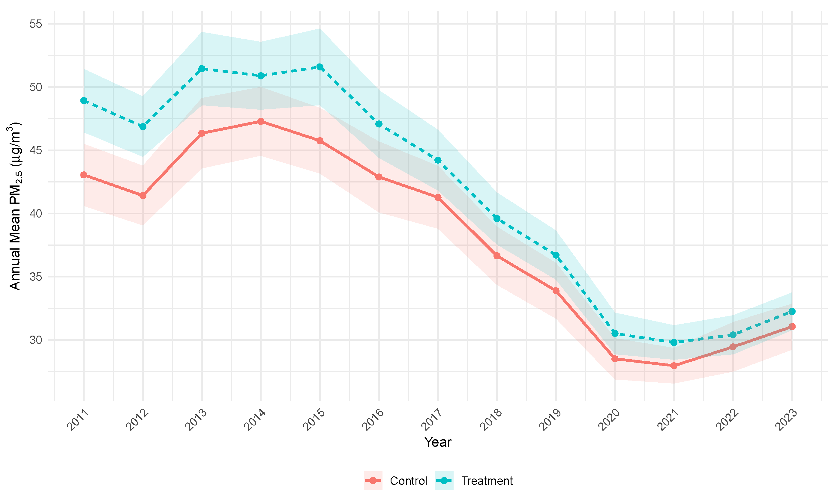
Figure 1 plots the annual mean PM_2.5 concentrations for treatment and control groups from 2011 to 2023. Both groups exhibit a broadly parallel downward trend, consistent with national-level air quality improvements driven by the 2013 Action Plan on Air Pollution Prevention and Control and subsequent policies [1]. The treatment group (cities that eventually established specialized environmental divisions) maintains slightly higher PM_2.5 levels throughout the period, consistent with governance specialization being adopted in more polluted jurisdictions. Visual inspection alone cannot establish causality given the staggered timing of treatment.

4.2. TWFE Baseline Results

Table 2 presents TWFE regression results for the harmonized 324-city sample, excluding the 10 cities with pre-panel adoption; Table S3 reports sensitivity results that recode their first treatment year to 2011. In Model (1), with no control variables, the coefficient on $Treated$ is $-0.037$ (SE $=0.014$, $p=0.011$). Adding basic province-level controls in Model (2) yields a coefficient of $-0.028$ (SE $=0.015$, $p=0.060$). Standard errors are clustered at the city level, reflecting the unit of treatment assignment.

Under city-level clustering, the TWFE estimate in the baseline specification achieves statistical significance at the 5% level. The progressive attenuation when adding controls (from $-0.037$ to $-0.028$) and the sensitivity of statistical significance to the clustering level (see Table S4) are consistent with the TWFE bias identified in the methodological literature. As we demonstrate below, the Goodman-Bacon decomposition reveals that this attenuation is partly driven by contaminated comparisons in which already-treated units serve as controls.

4.3. Callaway–Sant’Anna Main Results

The Callaway–Sant’Anna estimator yields an overall ATT of $-0.040$ (SE $=0.016$, $p=0.0097$), statistically significant at the 1% level. This corresponds to an approximately 3.9% reduction in PM_2.5 concentrations (computed as $exp(-0.040)-1=-0.039$). The result is substantively meaningful: given the mean PM_2.5 of 40.08 $\mathsf{\mu }$g/m³, a 3.9% reduction translates to approximately 1.56 $\mathsf{\mu }$g/m³, which has non-trivial health implications given the epidemiological evidence on PM_2.5 exposure thresholds [20].

4.4. Alternative Estimators

To guard against estimator-specific artifacts, we apply four complementary estimators to the harmonized 324-city sample.

Table 3. Comparison of four estimators on the harmonized 324-city sample.

Estimator	ATT	SE	p-Value
TWFE	$-0.037$ **	$\left(0.014\right)$	$0.011$
Callaway–Sant’Anna (DR)	$-0.040$ ***	$\left(0.016\right)$	$0.010$
Sun–Abraham	$-0.040$ ***	$\left(0.015\right)$	$0.009$
Borusyak–Jaravel–Spiess	$-0.054$ ***	$\left(0.016\right)$	$0.001$
Observations	4210

Dependent variable is ln(PM_2.5). All models estimated on the harmonized 324-city sample (excluding 10 pre-panel adopters). Standard errors (in parentheses) are clustered at the city level. CS-DID uses the doubly robust method with never-treated cities as the control group, universal base period, and multiplier bootstrap (seed = 42). ** $p<0.05$, *** $p<0.01$.

reports the results. All four produce negative, statistically significant treatment effects, with point estimates ranging from $-0.037$ (TWFE) to $-0.054$ (Borusyak–Jaravel–Spiess). The consistency across estimators that make different identifying assumptions strengthens the causal interpretation.

4.5. City-Level Control Robustness

A potential concern is that our baseline specification includes only province-level controls, which may fail to capture city-specific confounders. To address this, we augment the Callaway–Sant’Anna estimator with city-level baseline covariates through the outcome regression formula.

Table 4. CS-DID with city-level baseline controls.

Specification	ATT	SE	Cities
(A) No covariates (baseline)	$-0.040$ ***	$\left(0.016\right)$	324
(B) + Firm density (2011)	$-0.031$ **	$\left(0.015\right)$	313
(C) + GDP, tertiary, HDI (2013)	$-0.035$ **	$\left(0.016\right)$	255

Dependent variable is ln(PM_2.5). All models use the Callaway–Sant’Anna doubly robust estimator with never-treated control group and universal base period. City-level covariates enter through the outcome regression formula (xformla). City counts vary due to covariate availability. Bootstrap standard errors (in parentheses) reported with seed = 42. ** $p<0.05$, *** $p<0.01$.

reports three specifications: (A) the baseline without covariates, (B) adding baseline firm density as a proxy for industrialization, and (C) adding economic baseline characteristics (log GDP, tertiary sector share, and HDI, all measured at 2013 values to avoid bad control problems). The ATT ranges from $-0.031$ to $-0.040$ across specifications and remains statistically significant at the 5% level in all cases, confirming that the main result is not driven by omitted city-level confounders. A balance check in the Supplementary Materials shows that the 69 cities dropped from Spec C due to missing 2013 covariates are systematically less polluted, less urbanized, more industrially concentrated, and less likely to have adopted the reform, a pattern consistent with sparser HDI and tertiary-share coverage in western and inland prefectures. Two non-exclusive interpretations of the selection are available: dropped cities have lower detection power (less baseline pollution and lower treatment share), or they rely on alternative administrative enforcement (reflected in the largest imbalance, government-intervention |SMD| = 0.95) that could suppress PM_2.5 independently of the courts. Because Spec A on the full 324-city sample already yields a larger and statistically stronger ATT than Spec C ($-0.040$ vs. $-0.035$), neither interpretation shifts the main inference in favor of the finding; we anchor the main inference on Spec A and interpret Spec C as a conditional robustness check on a more homogeneous, higher-pollution subsample.

4.6. Event Study Analysis

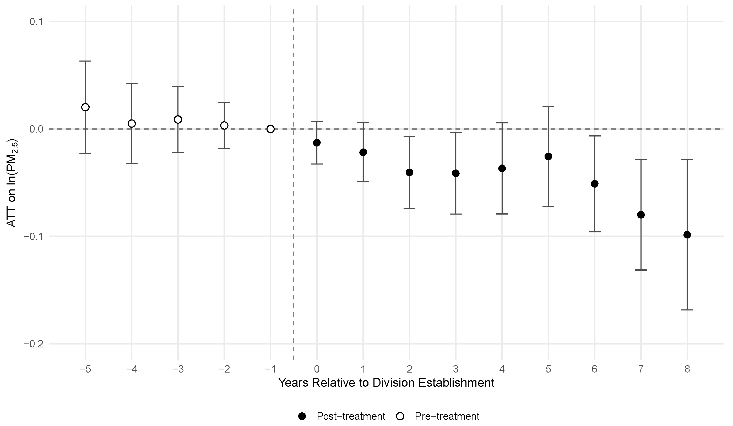
Figure 2 presents the dynamic ATT estimates from the Callaway–Sant’Anna event study, plotting treatment effects by years relative to the establishment of specialized environmental divisions ($e=-5$ to $e=8$).

The pre-treatment coefficients ($e=-5$ to $e=-1$) are small, statistically insignificant, and centered around zero, providing no evidence of differential pre-trends. This supports the parallel trends assumption. After treatment, coefficients turn consistently negative: PM_2.5 reductions appear promptly and persist over the medium term. The point estimates grow modestly over time, consistent with the idea that institutional capacity and reputational deterrence accumulate gradually.

4.7. TWFE Weight Decomposition

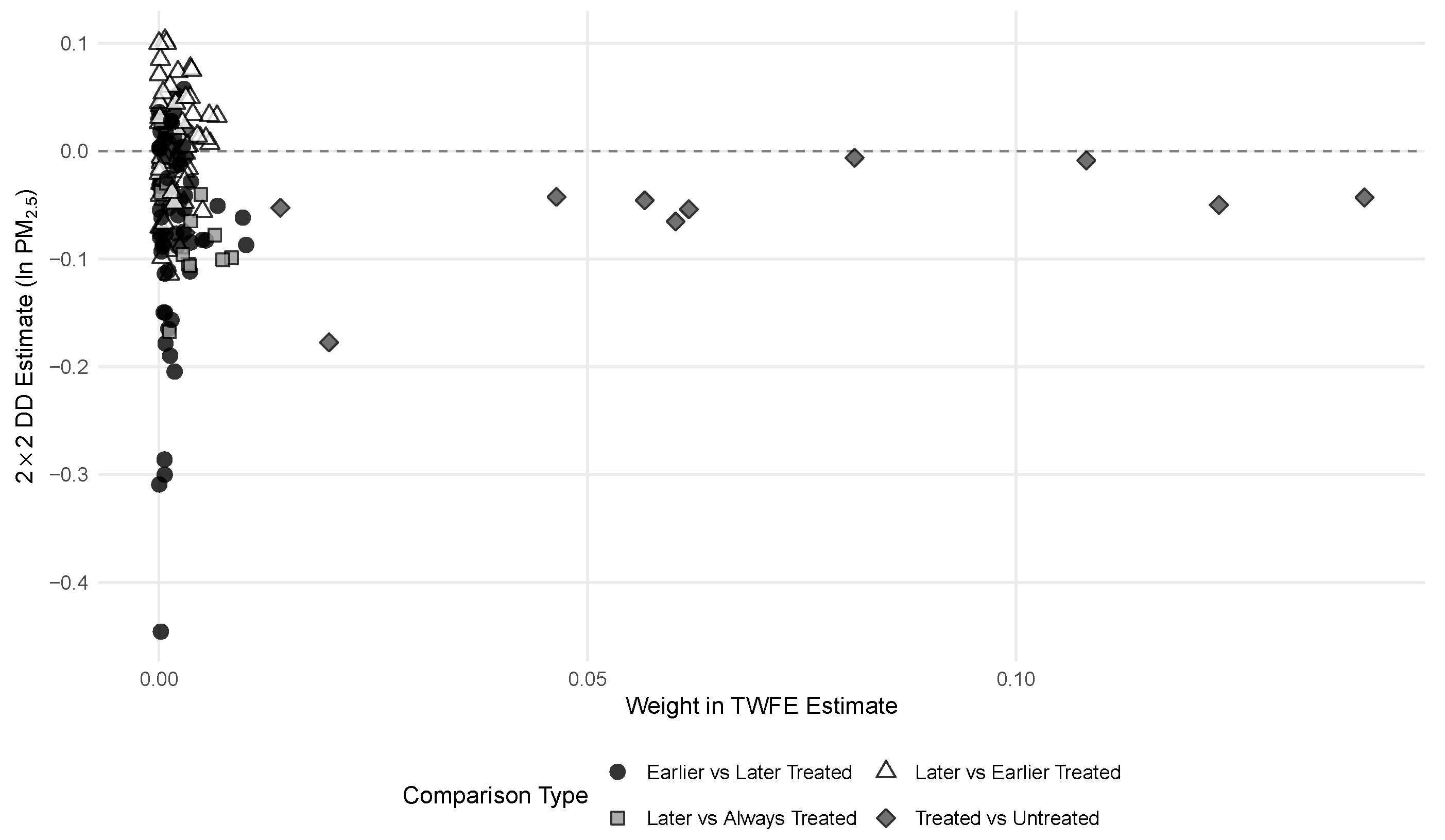
Figure 3 presents the Goodman–Bacon decomposition of the TWFE estimate. The decomposition reveals three types of $2\times 2$ comparisons: (i) treated versus never-treated, (ii) earlier-treated versus later-treated, and (iii) later-treated versus earlier-treated. The key insight is that comparisons using already-treated units as controls (type iii) contaminate the estimand, because those “control” units have already experienced treatment effects of their own. Under heterogeneous treatment dynamics, the resulting TWFE bias is not sign-determined a priori; the heterogeneity-robust estimators avoid this contamination by construction (see Roth et al. [11] for a formal treatment). In our data, the TWFE and heterogeneity-robust estimators nonetheless yield substantively similar negative ATTs (Table 3), suggesting that the decomposition-based concern, while important in principle, does not overturn the qualitative finding.

4.8. Robustness Checks

We subject the main finding to eight robustness dimensions, summarized narratively below; detailed tables appear in the Supplementary Materials.

(1) Alternative estimators. As reported in Table 3, four estimators making different identifying assumptions all yield negative, significant ATTs ($-0.037$ to $-0.054$), ruling out estimator-specific artifacts.

(2) Clustering sensitivity. The significance of the TWFE estimate depends on the clustering level: city-level clustering yields $p=0.011$, and two-way city+year clustering yields $p=0.047$. The Bell–McCaffrey CR2 small-sample correction for the TWFE estimate yields effective degrees of freedom of 20.5 and $p=0.181$ under province clustering (Table S2). Under province-level CR1 clustering, significance attenuates for all estimators: TWFE $p=0.173$, Sun–Abraham $p=0.125$, Borusyak–Jaravel–Spiess $p=0.078$, and CS-DID $p=0.289$ (Table S4). This is expected given only 31 provincial clusters. Both clustering choices have a theoretical basis. City-level clustering aligns with the unit of treatment assignment (each municipal court made its own adoption decision), while province-level clustering reflects the within-province correlation plausibly induced by the 2014 national directive’s role in catalyzing provincial adoption plans. We report city-level clustering as the primary specification given the individual-municipality decision unit, but present province-level results as an alternative baseline with its own defensible basis rather than as a purely conservative lower bound. At both levels, the effect is negative and substantively similar in magnitude; statistical significance is robust under city clustering and attenuated to the marginal range under province clustering given the small number of clusters.

(3) Alternative dependent variables. The CS-DID estimator applied to alternative pollution measures produces consistent results: ln(SO₂) (ATT $=-0.169$ **, $N=3416$), ln(PM_2.5) (ATT $=-0.042$ **, $N=1781$), heavy pollution days (ATT $=-3.83$ **, $N=2452$), and good air quality days (ATT $=+10.85$ ***, $N=2452$). The convergent evidence across pollutants rules out PM_2.5-specific measurement artifacts.

(4) EPL cohort splits. To disentangle the treatment effect from the 2015 Environmental Protection Law, we split the sample by EPL timing. The pre-2015 subsample (25 cities in the 2012–2014 treatment cohorts) yields ATT $=-0.079$ ** ($p=0.029$), while the post-2015 subsample (cohorts 2016 and later) yields ATT $=-0.025$ ($p=0.116$). Excluding the 2014–2015 cohorts entirely yields ATT $=-0.041$ ** ($p=0.012$). The persistence of a significant treatment effect in the pre-2015 subsample, where the EPL had not yet taken effect, is inconsistent with the hypothesis that the EPL alone drives the observed reduction, though the small number of pre-2015 treated cities warrants caution, and the large point estimate may partly reflect estimation noise in sparse cohort-time cells.

(5) Leave-one-cohort-out (LOCO). Sequentially dropping each of the 12 treatment cohorts, the CS-DID ATT remains negative and significant in all 12 specifications, ranging from $-0.029$ (dropping cohort 2013) to $-0.048$ (dropping cohort 2018); all 12 specifications are individually significant (Table S5), and the Supplementary Materials visualize the full set. No single cohort drives the overall result.

(6) Spatial spillover analysis. We report two specifications. Specification 1 uses the leave-one-out mean ln(PM_2.5) of all other same-province cities as the dependent variable; the CS-DID estimator yields a negative neighbor ATT of $-0.036$ ($p<0.001$; Table S6, Panel A; Figure S1). This specification, however, conflates genuine cross-city spillover with the own-treatment effect of neighbors that concurrently adopted the reform. Specification 2 restricts the neighbor pool to never-treated cities only; on this cleaner identification sample (319 of 324 cities; five focal cities are dropped because their province contains no never-treated neighbor) the CS-DID neighbor ATT attenuates to $-0.009$ ($p=0.528$) and the TWFE analogue is similarly null (Panel B). Crucially, on the same 319-city restricted sample the own-PM_2.5 effect remains negative and significant (CS-DID $-0.035$, $p=0.028$; Panel C), confirming the main finding under the cleaner sample. Two conclusions follow. First, there is no evidence of pollution displacement under either specification (displacement would require a positive neighbor ATT). Second, once the neighbor pool is purged of concurrently-treated cities, clean cross-city spillovers cannot be identified, indicating that the initial negative neighbor effect largely reflected neighbors’ own court adoption rather than transmission from the focal city. SUTVA is violated by this concurrent adoption, but the direction of bias on our main ATT is ambiguous rather than demonstrably conservative.

(7) City-level controls. As detailed in Section 4.5 (Table 4), all three covariate specifications retain significance at the 5% level, confirming that the main result is not driven by omitted city-level confounders; a balance check between retained and dropped cities appears in the Supplementary Materials.

(8) Pre-panel adopter sensitivity. Including the 10 cities that adopted before 2011 (recoded to cohort 2011) raises the TWFE ATT to $-0.039$ *** and the Sun–Abraham ATT to $-0.042$ *** on the full 334-city sample (Table S3). The results are quantitatively similar to the harmonized sample, confirming that the exclusion is conservative rather than consequential.

Taken together, six of the eight dimensions confirm robustness to estimator choice, outcome measure, policy confounds, sample composition, covariate specification, and pre-panel adopter inclusion. The clustering sensitivity analysis (dimension 2) reveals that significance depends on the clustering level, with province-level clustering yielding non-significant results for all estimators. The spatial analysis (dimension 6) reveals a SUTVA violation whose direction of bias is ambiguous rather than known-direction conservative, constituting a limitation that qualifies the causal interpretation (see Section 5).

4.9. Heterogeneity Analysis

Rather than splitting the sample into subgroups (which would severely reduce the statistical power of the Callaway–Sant’Anna estimator), we exploit the cohort structure of the CS-DID framework to examine heterogeneity. Specifically, we extract the group-specific ATTs (i.e., the average treatment effect for each cohort defined by the first observed treatment year used in the panel) and correlate them to cohort-level baseline characteristics. This approach maintains full methodological consistency with the main analysis while avoiding the small-sample problems inherent in subsample estimation.

Table 5. Cohort-specific ATTs from the Callaway–Sant’Anna Estimator.

Cohort	Cities	ATT	SE	p-Value	Mean IndStru	Mean PM2.5
2012	2	$-0.076$	$\left(0.066\right)$	$0.253$	0.741	50.89
2013	7	$-0.165$ **	$\left(0.077\right)$	$0.033$	0.849	49.53
2014	16	$-0.038$	$\left(0.033\right)$	$0.257$	0.881	47.46
2015	13	$-0.037$	$\left(0.049\right)$	$0.443$	0.759	54.38
2016	24	$-0.040$	$\left(0.027\right)$	$0.141$	0.690	54.43
2017	26	$-0.023$	$\left(0.027\right)$	$0.399$	0.709	51.82
2018	20	$+0.030$	$\left(0.033\right)$	$0.371$	0.712	43.76
2019	11	$-0.008$	$\left(0.054\right)$	$0.881$	0.799	42.83
2020	10	$-0.112$ ***	$\left(0.027\right)$	<0.001	0.732	47.60
2021	21	$-0.050$	$\left(0.032\right)$	$0.118$	0.713	50.69
2022	5	$-0.058$	$\left(0.044\right)$	$0.186$	0.760	48.66
2023	2	$+0.048$	$\left(0.048\right)$	$0.315$	0.774	45.57

Each row reports the group-specific ATT from the Callaway–Sant’Anna estimator for cities that established specialized environmental divisions in the indicated year. Mean IndStru and Mean PM_2.5 are cohort-level baseline averages calculated for cities in each cohort. Standard errors (in parentheses) are computed using the multiplier bootstrap. ** $p<0.05$, *** $p<0.01$.

reports the cohort-specific ATTs from the Callaway–Sant’Anna estimator. Of the 12 cohorts with estimable ATTs, 10 exhibit negative point estimates. Two cohorts achieve statistical significance: the 2013 cohort ($ATT=-0.165$, $p<0.05$) and the 2020 cohort ($ATT=-0.112$, $p<0.001$). The variation across cohorts (from $-0.165$ to $+0.048$) motivates investigation of what city-level characteristics predict larger treatment effects.

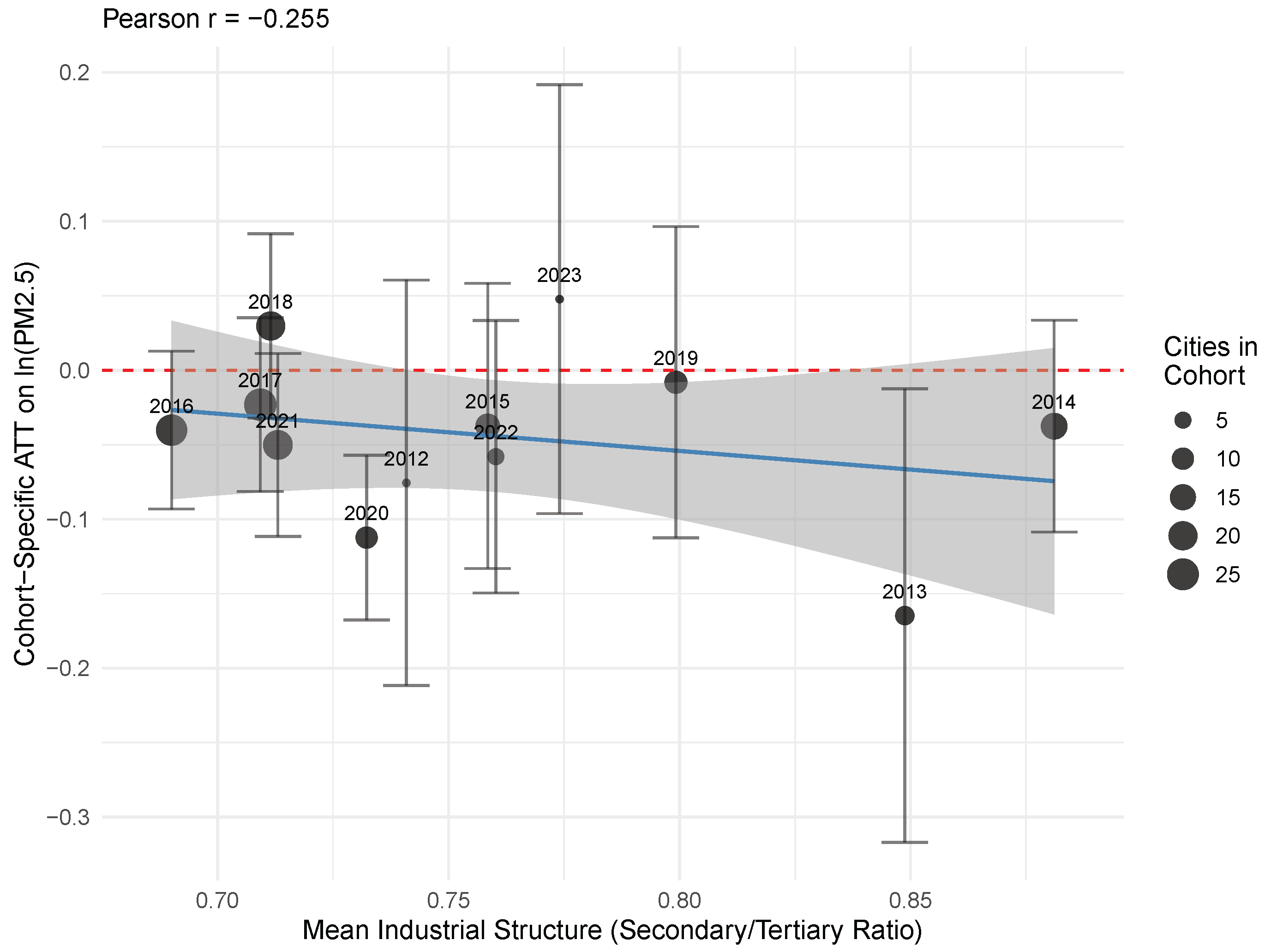
Figure 4 plots the relationship between cohort-level mean industrial structure and the cohort-specific ATT. Cohorts composed of more industrialized cities tend to exhibit larger pollution reductions ($r=-0.255$), and cohorts with higher baseline PM_2.5 concentrations show a similar pattern ($r=-0.360$). However, neither correlation is statistically significant at conventional levels ($n=12$ cohorts; a two-tailed test at $\alpha =0.05$ requires $\left|r\right|>0.576$). When we divide cohorts at the median of industrial structure, the weighted mean ATT for high-industrialization cohorts is $-0.047$, compared to $-0.032$ for low-industrialization cohorts. The direction of these associations is consistent with a deterrence hypothesis, but the small number of cohorts precludes definitive inference.

We emphasize that these correlations are suggestive rather than definitive, given the small number of cohorts ($n=12$) and the inherent imprecision of cohort-level averages. Nevertheless, the directional patterns are consistent with theory: environmental governance specialization appears to be most effective in cities with heavier industrial bases and higher baseline pollution levels, where the scope for deterrence and enforcement is greatest.

5. Discussion

5.1. Main Finding: Environmental Governance Specialization Reduces PM_2.5

Four complementary estimators consistently indicate that establishing specialized environmental adjudication divisions reduces PM_2.5 (Callaway–Sant’Anna point estimate: approximately 3.9%; the full range across the four estimators is 3.6–5.3%, with $p<0.05$ in all cases). Taking the Callaway–Sant’Anna point estimate of $-0.040$, the average city in our sample (PM_2.5 = 40.08 $\mathsf{\mu }$g/m³) would experience a decrease of roughly 1.56 $\mathsf{\mu }$g/m³. To put this in perspective, epidemiological studies estimate that a 10 $\mathsf{\mu }$g/m³ reduction in PM_2.5 can extend life expectancy by 0.6 years [20,21]. Even a partial improvement in this size carries real health consequences at scale.

5.2. Methodological Implications: TWFE Versus Robust Estimators

The divergence between TWFE and heterogeneity-robust estimates is not merely a technical issue. Under province-level clustering (a common choice given China’s administrative structure), TWFE estimates lose statistical significance; under city-level clustering, they are significant but attenuated relative to the robust estimators. The Goodman–Bacon decomposition traces the attenuation to “bad comparisons” in which already-treated cities serve as controls [8,11].

This matters beyond our specific application. Many environmental policy evaluations use TWFE to assess staggered rollouts (emissions trading, inspection regimes, clean production standards). Under heterogeneous treatment effects across adopting cohorts, as is likely in such settings, TWFE can produce biased estimates whose direction is not sign-determined a priori. Researchers evaluating staggered environmental policies should routinely apply heterogeneity-robust estimators as a diagnostic check regardless of the expected direction of bias.

5.3. Mechanisms and Channels

Our data do not support formal mediation analysis, but we provide limited evidence on two candidate channels. The most direct is environmental public interest litigation (EPIL). EPIL case count data are available only for 2018–2022, which severely limits what can be inferred. A TWFE specification restricted to this five-year window yields a positive but insignificant coefficient on governance specialization ($p=0.620$), reflecting limited statistical power over a short panel. We also attempted a CS-DID specification imputing pre-2018 EPIL counts as zero, but this approach is methodologically invalid because the zero-imputation mechanically generates a level shift at 2018 regardless of the treatment’s true effect, and we do not report it as evidence. In contrast, the effect on administrative penalties is small and statistically insignificant regardless of specification (ATT $=0.064$, $p=0.629$ for penalty counts; ATT $=0.009$, $p=0.964$ for penalty amounts). The mechanism regressions reported here cluster standard errors at the province level, following the original mechanism-analysis pipeline. A sensitivity check with city-level clustering (matching the main analysis) yields qualitatively identical null results on both penalty measures (smallest $p=0.37$) and an essentially identical EPIL TWFE null; see Supplementary Table S7. The insignificant penalty result, combined with the inability to credibly test the EPIL channel due to data limitations, means that the precise mechanism remains unidentified. We can rule out administrative penalties as the primary channel, but cannot affirmatively establish litigation as the driver.

A second candidate channel is deterrence. A specialized division credibly raises the expected cost of environmental violations, inducing firms to reduce emissions proactively [5]. The heterogeneity results offer directionally consistent but statistically inconclusive support: cohorts composed of more industrialized cities and those with higher baseline PM_2.5 tend to show larger pollution reductions ($r=-0.255$ for industrial structure, $r=-0.360$ for baseline pollution), but neither correlation is statistically significant at conventional levels given only 12 cohort-level observations. The pattern is consistent with a deterrence mechanism but cannot be treated as confirmatory evidence.

5.4. Addressing the 2015 Environmental Protection Law Confound

The revised Environmental Protection Law (EPL), effective January 2015, coincides with the peak period of governance specialization reform (2014–2021), raising potential confounding concerns. The 2014–2021 period witnessed a cascade of environmental policy instruments: the Air Pollution Prevention and Control Action Plan (2013), the revised EPL (2015), the Environmental Protection Tax Law (2018), and the revised Atmospheric Pollution Prevention and Control Law (2018). We address this multi-policy confound through four strategies.

First, year fixed effects absorb any nationwide policy shock that affects all cities uniformly, including the EPL and subsequent legislation. Second, the event study (Figure 2) shows no structural break around 2015; pre-treatment coefficients remain insignificant, and post-treatment effects accumulate gradually rather than jumping at EPL implementation. Third, our identification exploits city-level variation in the timing of division establishment, which the national policy timeline does not determine.

Fourth, and most directly, we split the sample by EPL timing. The pre-2015 subsample (25 cities in the 2012–2014 treatment cohorts) yields ATT $=-0.079$ ** ($p=0.029$), larger than the post-2015 subsample (cohorts 2016+; ATT $=-0.025$, $p=0.116$). The pre-2015 finding is informative: these cities experienced the pollution reduction before the EPL took effect, which is inconsistent with the hypothesis that the EPL alone drives the observed pollution reduction. The larger pre-2015 point estimate may partly reflect selection into early adoption by jurisdictions with stronger environmental commitments. Excluding 2014–2015 cohorts entirely yields ATT $=-0.041$ ** ($p=0.012$), virtually identical to the full-sample estimate.

5.5. Comparison with Existing Literature

Our study relates to, but differs from, several prior contributions. Zhang et al. [4] show that specialized divisions increase firm-level environmental expenditure, an important firm-level result that our city-level pollution evidence complements. Qi et al. [14] estimate a similar DID model but without heterogeneity-robust methods, leaving their estimates vulnerable to the biases we document. Wu et al. [6] find an association between environmental public interest litigation and urban pollution using yearbook data and explicitly call for objective measures and stronger identification, which our satellite-based approach provides. Among studies most closely related to ours, He and Qi [18] and Deng et al. [19] also document pollution reductions but rely on TWFE estimation; our heterogeneity-robust estimates confirm their directional findings while addressing the methodological limitations they share.

5.6. Limitations

Several limitations qualify our findings. The parallel trends assumption, though supported by the event study, remains untestable. We observe whether a city established a specialized division, but not how actively or competently it operates; operational quality surely varies across cities and over time, and our ATT averages over this heterogeneity. Satellite PM_2.5, while manipulation-proof, carries measurement error that may differ across regions [27]. Some controls are measured at the province rather than city level, leaving room for residual confounding, though our city-level baseline controls robustness check (Table 4) mitigates this concern. The 2020 treatment cohort contributes the largest and most significant cohort-specific ATT ($-0.112$, $p<0.001$), and we cannot fully rule out that COVID-19-related industrial shutdowns, which disproportionately affected manufacturing-intensive cities, contributed to this cohort’s estimated effect. Year fixed effects absorb the national component of the COVID-19 shock, but city-level heterogeneity in COVID-19 disruption remains a potential confound for this specific cohort.

The spatial analysis (Section 4, dimension 6) shows that neighbor PM_2.5 also declines under the unrestricted leave-one-out specification, but this effect disappears once the neighbor pool is restricted to never-treated cities only. This pattern indicates that most of the original negative neighbor effect reflected concurrent court adoption in neighboring cities rather than genuine spillover from the focal city; SUTVA is violated by this concurrent adoption, but the direction of bias on the main estimates is ambiguous rather than known-direction conservative. We therefore cannot assert that our main ATT is attenuated toward zero. Future work could exploit variation in caseload, staffing, or judicial quality, employ spatial econometric models, or use geographic discontinuities around province boundaries to separately identify direct and spillover effects.

5.7. Policy Implications

The policy takeaway is that institutional design choices matter for pollution outcomes. A PM_2.5 reduction of roughly 3.9% (3.6–5.3% across the four estimators) may sound modest in isolation, but applied across hundreds of cities over a decade, the cumulative health and economic benefits are substantial. The heterogeneity results sharpen the message: the largest gains come from prioritizing governance specialization in industrial cities with high baseline pollution, where the marginal abatement potential is greatest.

From a sustainability governance perspective, these findings illustrate a broader principle: durable environmental improvement requires not only stringent regulations but also institutional infrastructure capable of enforcing them. Governance specialization represents what the sustainability transitions literature terms “institutional innovation at the regime level” [3], embedding environmental expertise within the judicial system rather than relying solely on executive-branch enforcement. Whether province-level clustering of reform adoption generates genuine cross-city externalities, as distinct from concurrent provincial-level policy rollouts, is a question our data cannot cleanly resolve and warrants dedicated spatial-identification strategies in future work.

Beyond China, the finding that concentrating environmental expertise in dedicated units improves outcomes is relevant to any jurisdiction considering governance reform. Australia’s Land and Environment Court, India’s National Green Tribunal, and Kenya’s Environment and Land Court reflect similar institutional design choices [15]. The prerequisites–adequate technical training, sufficient caseload to sustain specialization, and complementary legal standing (such as public interest litigation)–are not unique to the Chinese system. The transferability of our results is limited, however, by China’s specific administrative structure, in which intermediate courts occupy a particular position within a unitary-state hierarchy. Whether similar reforms would be effective in federal systems or common-law jurisdictions requires separate investigation.

6. Conclusions

Under the identifying assumptions of our staggered difference-in-differences design, establishing specialized environmental adjudication divisions in China’s intermediate courts is associated with a reduction in local PM_2.5 of approximately 3.9% on average. Using satellite PM_2.5 data for 324 Chinese prefecture-level cities (2011–2023) and four complementary DID estimators, we consistently estimate PM_2.5 reductions ranging from 3.6% to 5.3% across estimators ($p<0.05$ in all cases under city-level clustering). The Goodman-Bacon decomposition attributes the modest gap between the TWFE and heterogeneity-robust estimates to contaminated comparisons in staggered adoption, while city-level controls and alternative dependent variables leave the result unchanged.

The parallel trends assumption is supported by event study evidence. Six of the eight robustness dimensions confirm the main finding: alternative estimators, alternative dependent variables, EPL cohort splits, leave-one-cohort-out, city-level controls, and pre-panel adopter inclusion. The remaining two dimensions qualify rather than overturn the result: province-level clustering attenuates significance given the small number of provincial clusters, and the spatial analysis reveals a SUTVA violation whose direction of bias cannot be determined. The effect is concentrated in more industrialized, more polluted cities, though the precise mechanism remains unidentified. Spatial analysis of same-province neighbors finds no evidence of pollution displacement; however, once the neighbor pool is restricted to never-treated cities, the apparent spillover disappears, indicating that the unrestricted negative neighbor effect largely reflected concurrent provincial adoption rather than cross-city transmission from the focal city. These results demonstrate that institutional design is a viable lever for improving air quality alongside command-and-control regulation, contributing to the broader sustainability transitions agenda by showing that governance specialization can complement regulatory instruments in achieving SDG targets for clean air. Tracking whether effects grow or decay as institutions mature and identifying the precise channels through which specialization operates are priorities for future work.

References

1. Geng, G.; Liu, Y.; Liu, Y.; Zheng, B.; Tong, D.; Li, M.; Zhang, Q.; He, K. Efficacy of China’s Clean Air Actions to Tackle PM2.5 Pollution between 2013 and 2020. Nat. Geosci. 2024, 17, 987–994. [Google Scholar] [CrossRef]
2. He, G.; Wang, S.; Zhang, B. Watering Down Environmental Regulation in China. Q. J. Econ. 2020, 135, 2135–2185. [Google Scholar] [CrossRef]
3. Markard, J.; Raven, R.; Truffer, B. Sustainability Transitions: An Emerging Field of Research and Its Prospects. Res. Policy 2012, 41, 955–967. [Google Scholar] [CrossRef]
4. Zhang, Q.; Yu, Z.; Kong, D. The Real Effect of Legal Institutions: Environmental Courts and Firm Environmental Protection Expenditure. J. Environ. Econ. Manag. 2019, 98, 102254. [Google Scholar] [CrossRef]
5. Zhang, L.; Su, L.; Liu, B.; Dai, Y. The Impact of Environmental Judicial Specialization on Corporate Greenwashing: Evidence from China. Sustainability 2026, 18, 1896. [Google Scholar] [CrossRef]
6. Wu, W.; Chan, P.C.H.; Lin, X. Urban Pollution Governance, Prosecutor-led Environmental Public Interest Litigation and Regional Environmental Disparities in China: Evidence from 282 Cities. China Int. J. 2024, 22, 73–95. [Google Scholar] [CrossRef]
7. Stern, R.E. Environmental Litigation in China: A Study in Political Ambivalence; Cambridge Studies in Law and Society, Cambridge University Press: New York, NY, USA, 2013. [Google Scholar] [CrossRef]
8. Goodman-Bacon, A. Difference-in-Differences with Variation in Treatment Timing. J. Econom. 2021, 225, 254–277. [Google Scholar] [CrossRef]
9. de Chaisemartin, C.; D’Haultfoeuille, X. Two-Way Fixed Effects Estimators with Heterogeneous Treatment Effects. Am. Econ. Rev. 2020, 110, 2964–2996. [Google Scholar] [CrossRef]
10. Sun, L.; Abraham, S. Estimating Dynamic Treatment Effects in Event Studies with Heterogeneous Treatment Effects. J. Econom. 2021, 225, 175–199. [Google Scholar] [CrossRef]
11. Roth, J.; Sant’Anna, P.H.C.; Bilinski, A.; Poe, J. What’s Trending in Difference-in-Differences? A Synthesis of the Recent Econometrics Literature. J. Econom. 2023, 235, 2218–2244. [Google Scholar] [CrossRef]
12. Greenstone, M.; He, G.; Jia, R.; Liu, T. Can Technology Solve the Principal-Agent Problem? Evidence from China’s War on Air Pollution. Am. Econ. Rev. Insights 2022, 4, 54–70. [Google Scholar] [CrossRef]
13. Callaway, B.; Sant’Anna, P.H.C. Difference-in-Differences with Multiple Time Periods. J. Econom. 2021, 225, 200–230. [Google Scholar] [CrossRef]
14. Qi, X.; Wu, Z.; Xu, J.; Sha, B. Environmental justice and green innovation: A quasi-natural experiment based on the establishment of environmental courts in China. Ecol. Econ. 2023, 205, 107700. [Google Scholar] [CrossRef]
15. United Nations Environment Programme. Environmental Courts and Tribunals—2021: A Guide for Policy Makers; Technical Report; UNEP: Nairobi, Kenya, 2021. [Google Scholar]
16. Meng, Y.; Yang, X. Environmental Justice Specialization and Corporate ESG Performance: Evidence from China Environmental Protection Court. Sustainability 2024, 16, 9531. [Google Scholar] [CrossRef]
17. Zheng, Y. Establishment of environmental protection courts, green finance, and corporate operating performance. Financ. Res. Lett. 2026, 90, 109301. [Google Scholar] [CrossRef]
18. He, L.Y.; Qi, X.F. Environmental Courts, Environment and Employment: Evidence from China. Sustainability 2021, 13, 6248. [Google Scholar] [CrossRef]
19. Deng, J.; Li, M.; Li, Y.; Lu, J. Effect of Environmental Courts on Pollution Abatement: A Spatial Difference-in-Differences Analysis. Sustainability 2024, 16, 1452. [Google Scholar] [CrossRef]
20. Ebenstein, A.; Fan, M.; Greenstone, M.; He, G.; Zhou, M. New Evidence on the Impact of Sustained Exposure to Air Pollution on Life Expectancy from China’s Huai River Policy. Proc. Natl. Acad. Sci. USA 2017, 114, 10384–10389. [Google Scholar] [CrossRef]
21. Chen, Y.; Ebenstein, A.; Greenstone, M.; Li, H. Evidence on the Impact of Sustained Exposure to Air Pollution on Life Expectancy from China’s Huai River Policy. Proc. Natl. Acad. Sci. USA 2013, 110, 12936–12941. [Google Scholar] [CrossRef]
22. Barwick, P.J.; Li, S.; Lin, L.; Zou, E. From Fog to Smog: The Value of Pollution Information. Am. Econ. Rev. 2024, 114, 1338–1381. [Google Scholar] [CrossRef]
23. Borusyak, K.; Jaravel, X.; Spiess, J. Revisiting Event-Study Designs: Robust and Efficient Estimation. Rev. Econ. Stud. 2024, 91, 3253–3285. [Google Scholar] [CrossRef]
24. Sant’Anna, P.H.C.; Zhao, J. Doubly Robust Difference-in-Differences Estimators. J. Econom. 2020, 219, 101–122. [Google Scholar] [CrossRef]
25. Hammer, M.S.; van Donkelaar, A.; Li, C.; Mudway, I.; Burnett, R.T.; van Erp, A.M.M.; Martin, R.V. Global Estimates and Long-Term Trends of Fine Particulate Matter Concentrations (1998–2018). Environ. Sci. Technol. 2020, 54, 7879–7890. [Google Scholar] [CrossRef] [PubMed]
26. van Donkelaar, A.; Hammer, M.S.; Bindle, L.; Brauer, M.; Brook, J.R.; Garay, M.J.; Hsu, N.C.; Kalashnikova, O.V.; Kahn, R.A.; Lee, C.; et al. Monthly Global Estimates of Fine Particulate Matter and Their Uncertainty. Environ. Sci. Technol. 2021, 55, 15287–15300. [Google Scholar] [CrossRef] [PubMed]
27. Wei, J.; Li, Z.; Cribb, M.; Huang, W.; Xue, W.; Sun, L.; Guo, J.; Peng, Y.; Li, J.; Lyapustin, A.; et al. Reconstructing 1-km-resolution High-Quality PM2.5 Data Records from 2000 to 2018 in China: Spatiotemporal Variations and Policy Implications. Remote Sens. Environ. 2021, 252, 112136. [Google Scholar] [CrossRef]
28. Cameron, A.C.; Miller, D.L. A Practitioner’s Guide to Cluster-Robust Inference. J. Hum. Resour. 2015, 50, 317–372. [Google Scholar] [CrossRef]
Figure 1. PM2.5 trends for treatment and control cities, 2011–2023. Shaded areas represent 95% confidence intervals. Treatment cities are those that established specialized environmental divisions at any point during the sample period.
Sustainability 18 05374 g001
Figure 2. Event study: dynamic treatment effects of environmental governance specialization on ln(PM2.5). Estimated using the Callaway–Sant’Anna (2021) estimator with doubly robust method. Error bars represent 95% confidence intervals based on the multiplier bootstrap. The dashed vertical line marks the treatment onset ( e = 0 ).
Sustainability 18 05374 g002
Figure 3. Goodman–Bacon decomposition of the TWFE estimate. Each point represents a 2 × 2 DID comparison, with horizontal position indicating its weight in the overall TWFE estimate and vertical position indicating the comparison-specific treatment effect estimate.
Sustainability 18 05374 g003
Figure 4. Cohort-specific ATT versus mean industrial structure. Each point represents a treatment cohort, with size proportional to the number of cities. The fitted line shows the OLS relationship ( r = 0.255 ). Error bars represent 95% confidence intervals. Cohorts with higher industrial structure (more pollution-intensive economies) tend to exhibit larger PM2.5 reductions.
Sustainability 18 05374 g004