Article

Electromobility Market Development in Selected European Countries: Long-Term Forecasts to 2035

by
Paweł Piotrowski
Electrical Power Engineering Institute, Warsaw University of Technology, Koszykowa 75 Street, 00-662 Warsaw, Poland
Sustainability 2026, 18(11), 5340; https://doi.org/10.3390/su18115340
Submission received: 3 April 2026 / Revised: 12 May 2026 / Accepted: 19 May 2026 / Published: 26 May 2026
(This article belongs to the Section Economic and Business Aspects of Sustainability)

Abstract

The article examines forecasts of electromobility development across seven European countries over a ten-year horizon (until 2035). The introduction provides a characterization and statistical analysis of the electromobility market within the framework of sustainable development. The analysis includes both leading electromobility markets and lower-income countries with relatively small electromobility sectors. First, forecasts for the total number of registered passenger vehicles of all drive types will be generated for each country, followed by forecasts for the number of passenger electric vehicles (Battery Electric Vehicle (BEV) and Plug-in Hybrid Electric Vehicle (PHEV)). Based on this data, the degree of electromobility development—defined as the percentage of passenger electric vehicles among all registered passenger vehicles through 2035—will be established. The forecasts will be conducted using an artificial intelligence model, a deterministic chaos theory model and selected trend extrapolation methods. The multi-stage approach applied to the problem, together with the use of single-type models within ensembles and the model selection procedure, constitutes an original, proprietary solution. To the author’s knowledge, a similar approach has not been reported for a forecasting task in the context of electromobility. Three ensemble projections will be presented: low, middle, and high. The article concludes with findings regarding the implementation of European Union (EU) sustainable development goals, specifically the degree of passenger vehicle electrification.

1. Introduction

The European Union’s electromobility objectives form part of the broader strategy of the European Green Deal and the “Fit for 55” legislative package [1,2]. Their overarching goal is to achieve climate neutrality by 2050.
The ban on the sale of new internal combustion engine vehicles (2035) is the EU’s most important and most concrete target. From 1 January 2035, all new passenger cars and light commercial vehicles sold on the EU market must be zero-emission [3]. In practice, this means a ban on the registration of new petrol- and diesel-powered vehicles (including both conventional hybrids and plug-in hybrids). An exception applies to synthetic fuels: following pressure from, among others, Germany, the possibility of selling internal combustion vehicles after 2032 was allowed, provided that they are powered exclusively by climate-neutral synthetic fuels (e-fuels), although this technology is currently still under development.
The second objective concerns CO2 emissions reduction. The EU has established intermediate milestones intended to compel manufacturers to gradually expand their electric vehicle offerings before 2035 [4]. In the case of passenger cars, a 55% reduction in CO2 emissions (relative to 2021 levels) is expected by 2030, while a 100% reduction in CO2 emissions is expected by 2035. An important element of this strategy is the Alternative Fuels Infrastructure Regulation (AFIR), which requires Member States to ensure that, by 2026, charging areas for passenger cars are located at intervals of no more than 60 km along the main trans-European transport network (TEN-T) corridors. In addition, for every registered battery electric vehicle (BEV), each Member State must provide 1.3 kW of power in the public charging network. These requirements are, unfortunately, difficult and costly for many European countries, particularly the less affluent ones.
Naturally, the risks and barriers cannot be overlooked. These include, among others, energy prices—high electricity costs in some countries (e.g., Germany) may slow the pace of fleet replacement; electricity grids—the need to modernize the grid so that it can withstand the simultaneous charging of millions of vehicles, particularly in cities, constitutes a major challenge; and the expansion of costly charging infrastructure. Another important issue is the impact of the growing share of EVs on power systems. Article [5] examines this issue in several European countries and shows that the climate benefits of electromobility depend strongly on the carbon intensity of the electricity mix.
Forecasts for the development of electromobility in Europe by 2032 point to a historic turning point. According to scenarios, 2032 will be the year in which the sales of fully electric vehicles (BEVs) will, for the first time, exceed a 50% share of the new car market across Europe [6]. This, of course, does not refer to the number of active passenger vehicles, but rather to the percentage of new registrations in 2032. In the case of Europe’s leader, Norway, the share of newly registered EVs had already exceeded 90% by 2025. Moreover, by 2030, the country plans to implement a complete ban on the sale of internal combustion vehicles. According to current plans, the primary market will be 100% electric by 2032 in Norway. The United Kingdom is currently surpassing Germany in terms of growth dynamics among the large markets. Owing to the British Zero-Emission Vehicle (ZEV) mandate, the United Kingdom has adopted some of the most stringent requirements in Europe: 80% of new cars and 70% of new vans are to be zero-emission by 2030, and 100% by 2035 [7]. Furthermore, BloombergNEF [8] indicates that the UK is the leader among large European markets, and that the share of EVs in new car sales there may reach 40% as early as 2026.
The development of electromobility across different countries has been the subject of extensive research. In the recent literature (2022–2025), forecasting the number of electric vehicles has evolved along three main lines of inquiry: sales forecasting, stock/ownership forecasting, and integrated models that link the growth of the EV fleet with charging infrastructure or energy demand. In the sales-oriented stream, both statistical models and machine-learning approaches have been applied. By contrast, studies concerned with forecasting the number of EVs in use are dominated by approaches combining grey models, Bass diffusion, system dynamics, or Long Short-Term Memory (LSTM)/Seasonal AutoRegressive Integrated Moving Average (SARIMA) methods. These studies indicate that the growth in EV numbers depends not only on historical data, but also strongly on public policy, cost-related factors, and infrastructure constraints.
In article [9], the authors propose a model to forecast EV sales volume and growth rates worldwide and in China (up to and including 2028), using both statistical and machine-learning methods by combining principal component analysis with a general regression neural network, based on the previous 11 years of EV sales data. A comprehensive review of forecasting methods for the number of EVs, including a comparison of past forecasts with their actual realization, is provided in article [10]. The study reported in [11] uses monthly EV sales data for India from 2018 to 2023 and compares AutoRegressive Integrated Moving Average (ARIMA) models with exponential smoothing methods. The bibliometric study presented in [12] organizes the main research streams related to EV adoption and sustainability on the basis of literature indexed in the Scopus database. Although it does not provide its own forecast of EV numbers, it is methodologically valuable for identifying dominant forecasting approaches and research gaps. In turn, the study described in [13] proposes a three-stage method for forecasting EV penetration in countries where motorization has not yet reached saturation. For Turkey, it was estimated that the number of electric passenger cars could range from 19.2 to 51 million by 2060, depending on the economic growth scenario. The study presented in [14] forecasts the stock of battery electric vehicles (BEVs) and plug-in hybrid electric vehicles (PHEVs) in the United States up to 2030 using an optimized grey model DGM (1,1,α). The authors estimate that the EV stock in the United States may reach approximately 30 million vehicles. In study [15], an Improved Bass Model based on Product Value (IBMPV) was developed for forecasting sales of new energy passenger vehicles. The authors demonstrate that including the variable “product value” improves model fit and predictive performance relative to the classical Bass, Gompertz, and Logistic models. The authors of article [16] analyse EV sales data, market volatility, and short-term forecasting, emphasizing the importance of transparent data and the limitations of long-term forecasting in a highly regulated market. Study [17] combines the grey model GM (1,1) with Bass diffusion and estimates the medium- and long-term number of EVs used by urban residents. Article [18], in turn, models future vehicle stocks and transport energy demand under different EV penetration and public-policy scenarios. Meanwhile, the authors of article [19] propose the deep-learning model EVs-PredNet for forecasting EV demand and compare it with classical regression-based methods. Study [20] estimates the number of electric vehicles and charging stations in Sakarya Province, Türkiye, for 2030 using advanced artificial-intelligence time-series methods and statistical approaches. Finally, study [21] explores the influential factors affecting electric vehicle sales through an extensive literature review and identifies the relative importance of these factors in EV sales forecasting.
In this study, BEVs and PHEVs are analysed jointly as active registered electric passenger vehicles. This aggregation was adopted to ensure cross-country comparability and to focus on the overall degree of passenger-vehicle electrification. Nevertheless, BEVs and PHEVs may follow different future trajectories, especially because policy frameworks increasingly distinguish between zero-emission vehicles and plug-in hybrid vehicles. Therefore, separate BEV and PHEV forecasting would be a valuable extension of the present study, provided that harmonized and sufficiently long country-level time series are available.
The empirical analysis covers seven European countries: Germany, Poland, France, Norway, Spain, the Czech Republic, and the United Kingdom. These countries were selected to represent different stages of electromobility development: relatively low EV penetration markets, medium-penetration large European markets, and Norway as a highly advanced benchmark case. The historical analysis is based on annual data for 2010–2025 inclusive (16 years), while the forecasting horizon covers 2026–2035. The analysed variable is the number of active registered electric passenger vehicles, defined as the combined stock of BEVs and PHEVs. In the final stage, this series is related to the total number of active registered passenger vehicles across all drivetrain types in order to calculate the projected EV share. The country-level historical time series used in this analysis are provided in the Supplementary Materials.
The primary objectives of this study are:
(I)
To conduct a statistical analysis comparing the dynamics and degree of electromobility development across seven selected European countries using historical data from 2010 to 2025 inclusive.
(II)
To perform forecasts of total passenger vehicle registrations across all drivetrain types for the period 2026 to 2035 inclusive.
(III)
To generate electromobility development forecasts (number of active registered EVs, including BEVs and PHEVs) for 2026–2035 using an original methodology based on three different ensemble models derived from five out of seven distinct single models across three ensemble projections.
(IV)
To analyse the percentage share of EVs (BEVs and PHEVs) in individual countries and to assess the feasibility of these forecasts across three distinct time horizons (1, 5, and 10 years ahead).
The multi-stage approach applied to the problem, combined with the use of single-type models within ensembles and the model-selection procedure, constitutes an original methodological solution.

2. A Statistical Assessment of Electromobility Development Levels and Growth Dynamics for Selected European Countries

Throughout this section, the term electric passenger vehicles refers to active registered passenger BEVs and PHEVs. The analysis therefore concerns vehicle stock rather than annual new sales or new registrations.
The development of electromobility across the analysed countries is not uniform. On the one hand, the situation can be assessed in terms of the absolute number of registered electric passenger vehicles (BEVs and PHEVs), in which case Germany, the United Kingdom, and France lead among the countries considered—Figure 1. However, the level of advancement is more accurately reflected by the share of these vehicles within the total passenger car fleet, irrespective of powertrain type. From this perspective, the seven analysed countries can be grouped into three categories:
  • A low level of electromobility development (Poland, 1.1%; Czech Republic, 1.4%; Spain, 2.6%);
  • A medium level of electromobility development (Germany, 6.4%; France, 6.2%; United Kingdom, 7.5%);
  • A high level of electromobility development (Norway, 35.6%).
As a preliminary analysis, Pearson linear correlation coefficients (R) were calculated between all seven countries to identify the pairs exhibiting the highest and lowest R values. Table 1 presents the results in the form of a cross-correlation matrix for the seven analysed countries. The six largest R values are highlighted in blue, while the six smallest R values are highlighted in red. All R values are statistically significant at the 0.05 level (p < 0.05).
Based on the results presented in Table 1, the following conclusions can be drawn by observing the correlations highlighted in blue (highest values) and red (lowest values): Norway’s correlations with other countries are the lowest; Spain exhibits the highest correlation values with the Czech Republic, France, and the United Kingdom; Germany has the highest correlation with France, while Poland shows its strongest correlation with the Czech Republic. Since the analysis concerns cumulative time series that increase over time, such a correlation matrix has, to some extent, limited interpretive value: it is difficult to infer from it the actual similarity of development mechanisms, although at the same time it is clear that examining the largest and smallest values of R produced logically consistent results.
To enable a robust comparison of the variability patterns (dynamics) of time series that differ by orders of magnitude (e.g., hundreds of thousands of registered electric passenger vehicles (BEVs and PHEVs) in Poland versus millions in Germany), the most effective approach is to map them onto a common scale without distorting the underlying trend structure. For this reason, three distinct time-series normalization methods were applied to assess cross-country differences among the analysed cases.
The first method is Min–Max normalization (0–1 scaling). This is the most suitable approach for comparing the stage of development along an S-shaped diffusion trajectory across countries. Its key advantage is that each series is anchored at 0 and capped at 1, which allows for a direct overlay of trajectories and facilitates assessing whether, for example, Poland in 2024 follows a similar growth shape to Germany in 2015. The Min–Max normalisation is defined by Equation (1).
x n o r m = x x m i n x m a x x m i n
where x is the original (raw) value of the variable to be normalized, x m i n is the minimum value of x in the reference set, x m a x is the maximum value of x in the reference set and x n o r m is the normalized value.
Figure 2 shows Min–max-normalized time series of the number of active registered electric passenger vehicles (BEVs and PHEVs) from 2010 to 2025 (inclusive) for seven analysed European countries. In Figure 2, it is clearly evident that Norway is at a completely different stage of the development cycle than the other analysed countries—the country’s curve exhibits a distinct shape, suggesting the initiation of a transition from a phase of rapid growth to a phase of gradual saturation of the process. Another observation is the lower position of the curves for Poland, Czech Republic, and Spain (i.e., countries with a low level of electromobility development) relative to the remaining countries. The trajectory for Germany also differs slightly (with a higher placement) compared with France and the United Kingdom, indicating the onset of a shift from rapid growth toward gradual market saturation.
The second normalization approach applied is indexing (base year = 100). This method converts an absolute time series into a relative measure of change, which facilitates the comparison of growth dynamics across countries or indicators that differ in units and magnitude. The procedure is scale-invariant: multiplying all raw values by a constant does not affect the index, because the constant cancels out in the ratio. However, the results are sensitive to the choice of the base year. The indexing normalization (base year = 100) is defined by Equation (2).
I t = x t x 0 · 100
where I t is the index value at time t, expressed relative to the base year where the index equals 100, x t is the original (raw) value of the indicator in period t, x 0 is the raw value in the base year (baseline period), t is time period (year) and 0 is the base year (2010).
Figure 3 shows Indexing-normalized time series of the number of active registered electric passenger vehicles (BEVs and PHEVs) from 2010 to 2025 (inclusive) for seven analysed European countries.
When analysing the dynamics and growth rates since 2010, Poland stands out clearly among the seven analysed countries, exhibiting the highest dynamics and the fastest growth of the process. France ranks second in this respect, followed by the Czech Republic and Spain. The remaining countries (Norway, Germany, and the United Kingdom) display markedly lower growth dynamics than the other analysed countries.
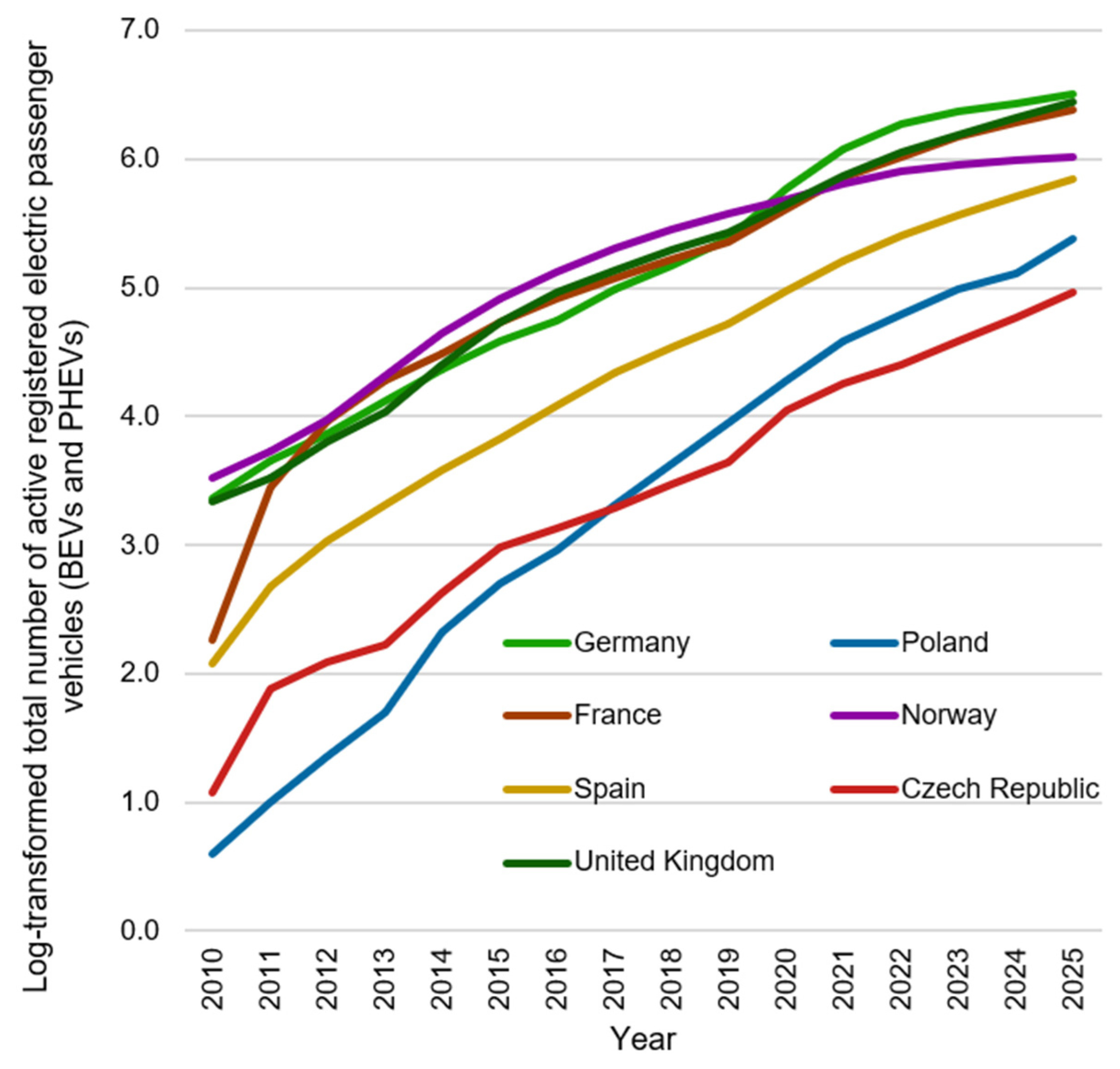
The third normalization method applied is the logarithmic scale (log transformation). It is useful for comparing percentage growth rates rather than absolute increases [22]. On a logarithmic scale, a constant growth rate (e.g., +20% year-on-year) appears as a straight line, which enables a direct comparison of the trend “slope”. If the lines for different countries are approximately parallel, this indicates that they are growing at the same percentage rate despite substantial differences in absolute levels. The logarithmic-scale normalization (log transformation) is defined by Equation (3).
y t = l o g b ( x t )
where y t is the log-transformed value at time t, x t is the original (raw) value of the indicator in period t, l o g b is logarithm with base b (b = 10) and t is time period.
Figure 4 shows log-transformed (logarithmic-scale) time series of the number of active registered electric passenger vehicles (BEVs and PHEVs) from 2010 to 2025 (inclusive) for seven analysed European countries. When examining the stability of the growth rate in Figure 4, it can be observed that Poland and the Czech Republic have exhibited similar growth rates over the last five years, and these rates are higher than, for example, in the case of Spain. The growth rate has declined most markedly over the last ten years in Norway. In the case of Germany, substantial changes in the trajectory are visible from 2020 onward—over the last five years, the pace of development has clearly slowed. The United Kingdom stands out from the other analysed countries by exhibiting a very stable and steady growth rate.
It should be emphasized that the normalization procedures were used only for exploratory and comparative purposes. They were not used as input transformations in the forecasting models, which were estimated separately for each country using the original EV-stock time series. Min–Max normalization was applied to compare the relative stage and shape of diffusion trajectories, indexing was used to compare cumulative growth dynamics relative to the base year, and logarithmic transformation was used to compare approximate percentage-growth patterns. Thus, normalization was not required for forecasting itself, but it provided additional insight into cross-country differences before the modelling stage. Stationarity testing was considered but not used as a decisive modelling criterion, because the analysed variables are cumulative EV-stock series and therefore represent a non-stationary diffusion process by construction.

3. Methods and Results

The forecasting procedure in this study consists of three clearly separated stages. First, the total number of active registered passenger vehicles, irrespective of drivetrain type, is forecast for each country for 2026–2035. This provides the denominator for the final EV-share calculation. Second, the number of active registered electric passenger vehicles, defined as BEVs and PHEVs, is forecast using seven single models and three ensemble variants. This provides the numerator for the final EV-share calculation. Third, the projected share of EVs in the total active passenger vehicle fleet is calculated as the ratio between the forecasted EV stock and the forecasted total passenger-vehicle stock. Thus, the study does not forecast three independent phenomena, but rather applies a sequential procedure leading from vehicle-stock forecasts to EV-share projections.
This section briefly describes the proposed forecasting methods and presents the results for 11 models. The Method of Constant Annual Growth (CAG), the first of the described approaches, was applied to forecast the total number of active passenger vehicle registrations for both internal combustion engine (ICE) and electric vehicle (EV) drivetrains from 2026 to 2035. This model was consistently utilized for each of the seven analysed countries. The subsequent group consists of seven individual (single) formula-based models. The parameters for these models were calibrated using optimization techniques, followed by a 10-step forward extrapolation to generate projections for the 2026–2035 period.
For each of the seven models used to forecast the development of electromobility with a 10-year horizon, the procedure was as follows:
  • In the first step, after calibrating the model parameters using an optimizer (through RMSE minimization over the 2010–2021 period), the model was employed to forecast the total number of active passenger electric vehicle registrations (BEV and PHEV) for 2022–2025, which served as a four-year validation horizon. The purpose of this step was to assess model performance over the last four observed years by evaluating the RMSE for that period and, if necessary, decide whether the model should be discarded,
  • In the second step, following the decision to retain the model, the parameters were recalibrated using an optimizer (through RMSE minimization over the full historical period of 2010–2025). The model was subsequently used to forecast the total number of active passenger electric vehicle registrations (BEV and PHEV) for the 2026–2035 period.
All forecasts using single-type models were performed using the Python version 3.9.7 environment. The final three methods are ensemble models, each incorporating five out of the seven individual models. For each country, the ensemble selection was performed by discarding the models that generated the highest and lowest forecast values. Each of the three ensemble models employs a unique weighting scheme to aggregate the outputs of the five constituent individual models. The sequential steps of the performed research are shown in Figure 5.
It should be emphasized that the forecasting framework adopted in this study is intentionally univariate. The models use historical time series of active registered passenger EVs, and the final EV-share calculations additionally use forecasts of the total number of registered passenger vehicles. Other potentially important explanatory variables, such as electricity prices, charging-infrastructure costs, subsidy schemes, vehicle prices, household purchasing power, fuel prices, and policy changes, are not included directly in the model equations.
This decision results primarily from the limited availability of long, harmonized, and comparable annual datasets for all seven countries over the full historical period. These factors are therefore treated as contextual drivers and sources of uncertainty rather than as quantitative predictors. Consequently, the forecasts should be interpreted as trend-based projections conditional on the continuation of the historical development mechanisms embedded in the observed EV time series.
To facilitate comparison of the forecasting methods, Table 2 summarizes the intuition, key parameters, optimization method, and role of each model in the forecasting framework.
To assess the quality of particular forecasting models within their parameter estimation ranges, the evaluation criterion Root Mean Square Error (RMSE) is used [23]. Root Mean Square Error is calculated by Equation (4). RMSE is sensitive to large errors and is more useful when large errors are particularly undesirable.
R M S E = 1 n i = 1 n ( y i y ^ i ) 2
where y ^ i is the predicted value, y i is the observed value, and n is the number of prediction points.
Although the present study uses RMSE for model estimation and weighting, future extensions may report normalized RMSE or another percentage-based error measure to improve cross-country comparability of model performance.

3.1. Method of Constant Annual Growth (CAG)

Method of Constant Annual Growth is described by Equation (5) [23]. Annual growth is the average annual growth rate based on historical data of the forecasting exercise. Forecasts are conducted by a Stepwise Method (2026–2035).
y ^ t = y ^ t 1 + j = 2 k ( y j y j 1 ) k 1
where k is the number of the data points in the time series and y j 1 is the previous value (or forecast) from the time series.
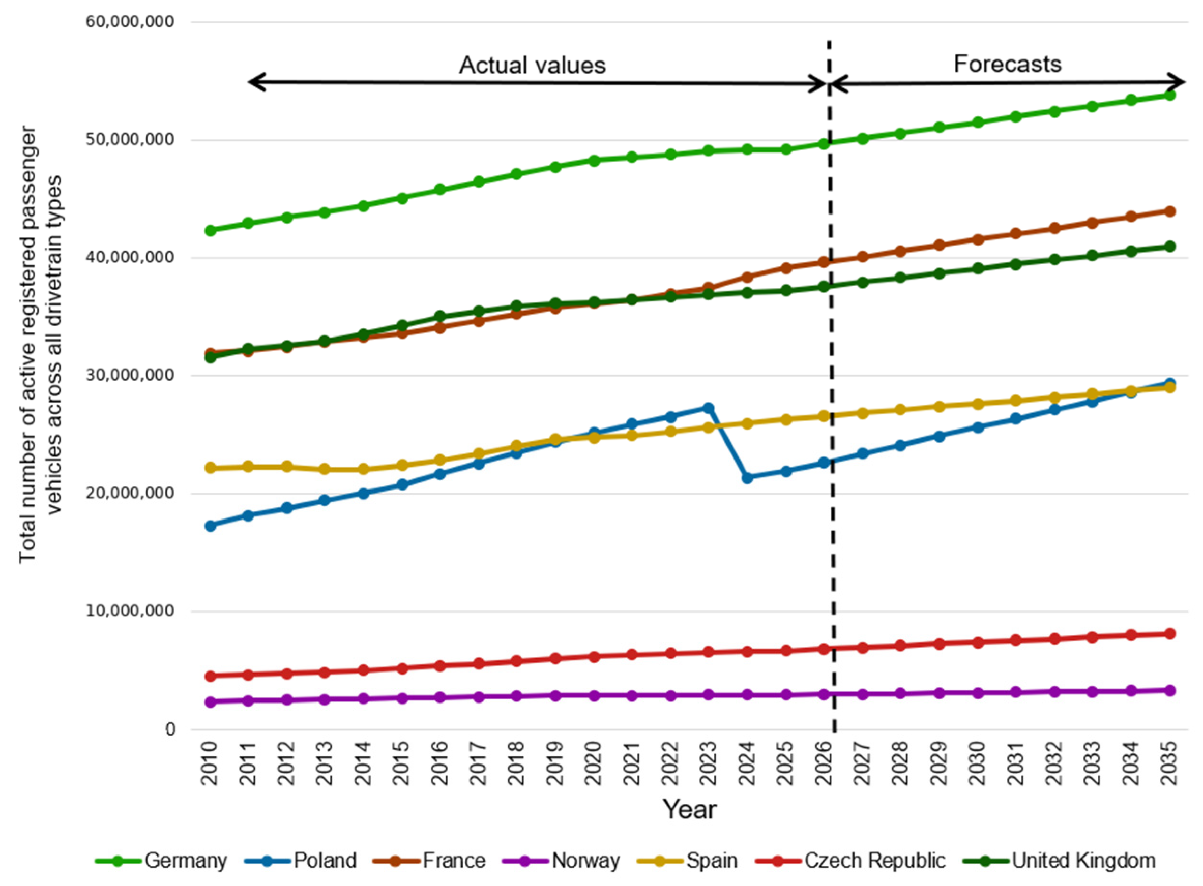
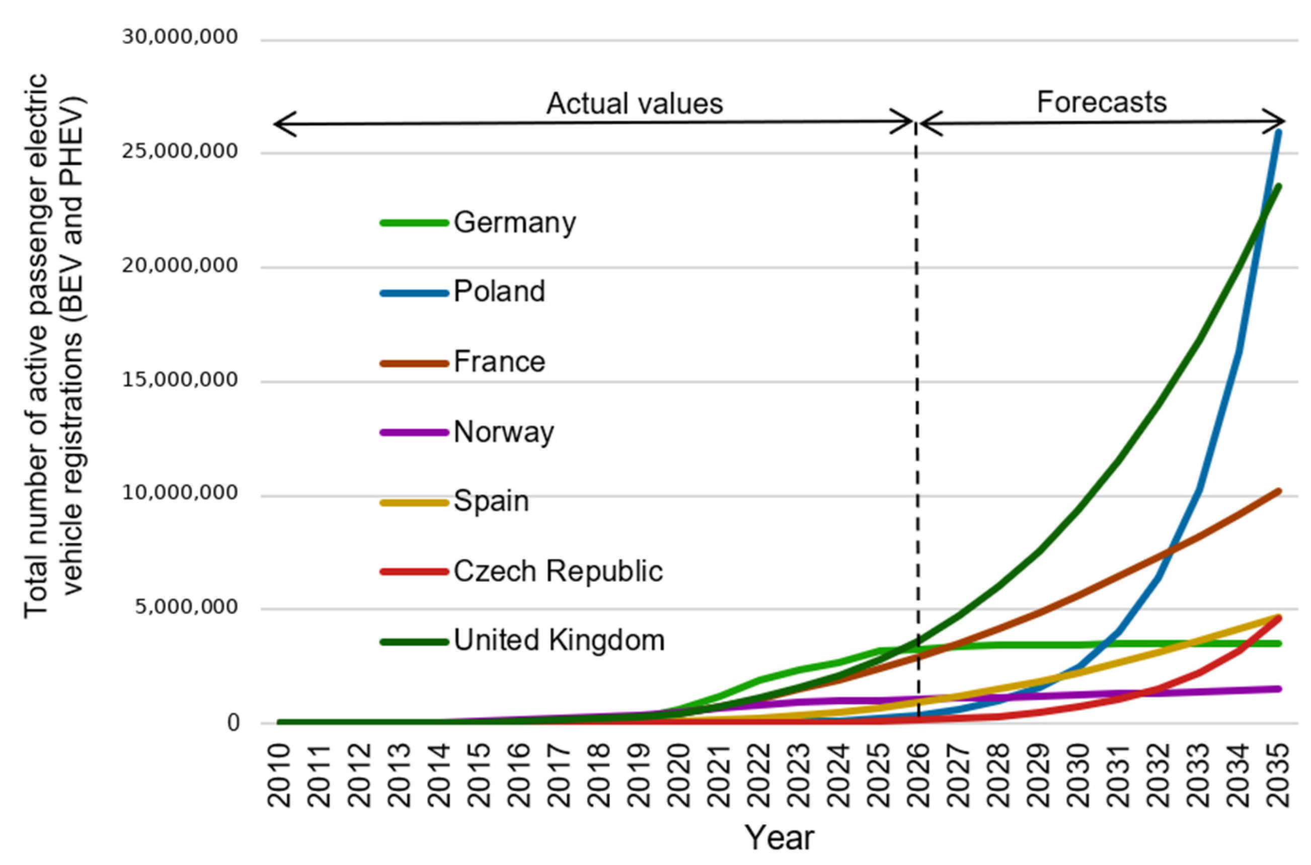
In the first step (Phase 1), the CAG model was used to forecast the total number of active registered passenger vehicles across all drivetrain types for the 2026–2035 period, based on historical data from 2010 to 2025 inclusive. The model was applied independently using data from seven countries. Given the relatively similar temporal variability and the slow growth dynamics of active passenger vehicle registrations across all seven countries, it was deemed appropriate to employ the same CAG model for all analysed jurisdictions. Figure 6 depicts the actual values and the forecasts for the total number of active registered passenger vehicles across all drivetrain types, as generated by the CAG model for the seven European countries under study.
Based on the historical data analysis of the seven studied countries, Germany and Poland demonstrate the most significant growth momentum. In the case of Poland, a notable and atypical decline in the number of registered passenger vehicles was observed in 2024. This phenomenon resulted from a regulatory decision to terminate inactive registrations. The Central Vehicle and Driver Register (CEPiK) automatically purged records of vehicles that had lacked both a valid technical inspection and mandatory third-party liability insurance for more than 10 years (referred to as ‘archival records’). Consequently, nearly 6 million entries were removed from the database, leading to a drastic statistical reduction in the total vehicle fleet size. It is important to note that although this represents a sharp numerical drop, these vehicles had physically been inactive and out of service for a prolonged period. To ensure the stability of the CAG model, the one-time negative differential between 2024 and 2023 was excluded from the calculations. Moreover, historical data from the period preceding the year in which the abrupt change occurred in Poland were adjusted accordingly in order to ensure a more appropriate (more realistic) value of the average annual change calculated using Equation (5). It should be also emphasized that the study did not compute the EV market penetration rate using historical data through 2023. Doing so would inevitably understate the historical level of electromobility development in Poland prior to 2024.

3.2. Damped Trend Exponential Smoothing Model (DTES)

The standard Holt’s linear method often tends to over-extrapolate trends indefinitely, which leads to unrealistic results for physical markets (such as the automotive industry). The Damped Trend Method (Holt’s method with damping) is defined by the following equation [23,24,25]:
L t = Y t + ( 1 ) ( L t 1 + φ T t 1 ) T t = β L t L t 1 + ( 1 β ) φ T t 1 y ^ t + h = L t + i = 1 h φ i T t
where L t is the estimate of the level of the series at time t, T t is the estimate of the trend (slope) of the series at time t, y t is the observed value at time t, α is the smoothing parameter for the level (0 < α < 1), β is the smoothing parameter for the trend (0 < β < 1), φ is the damping coefficient (0 < φ < 1), h is the forecast horizon (number of periods ahead) and y ^ t + h is the forecast for h steps ahead.
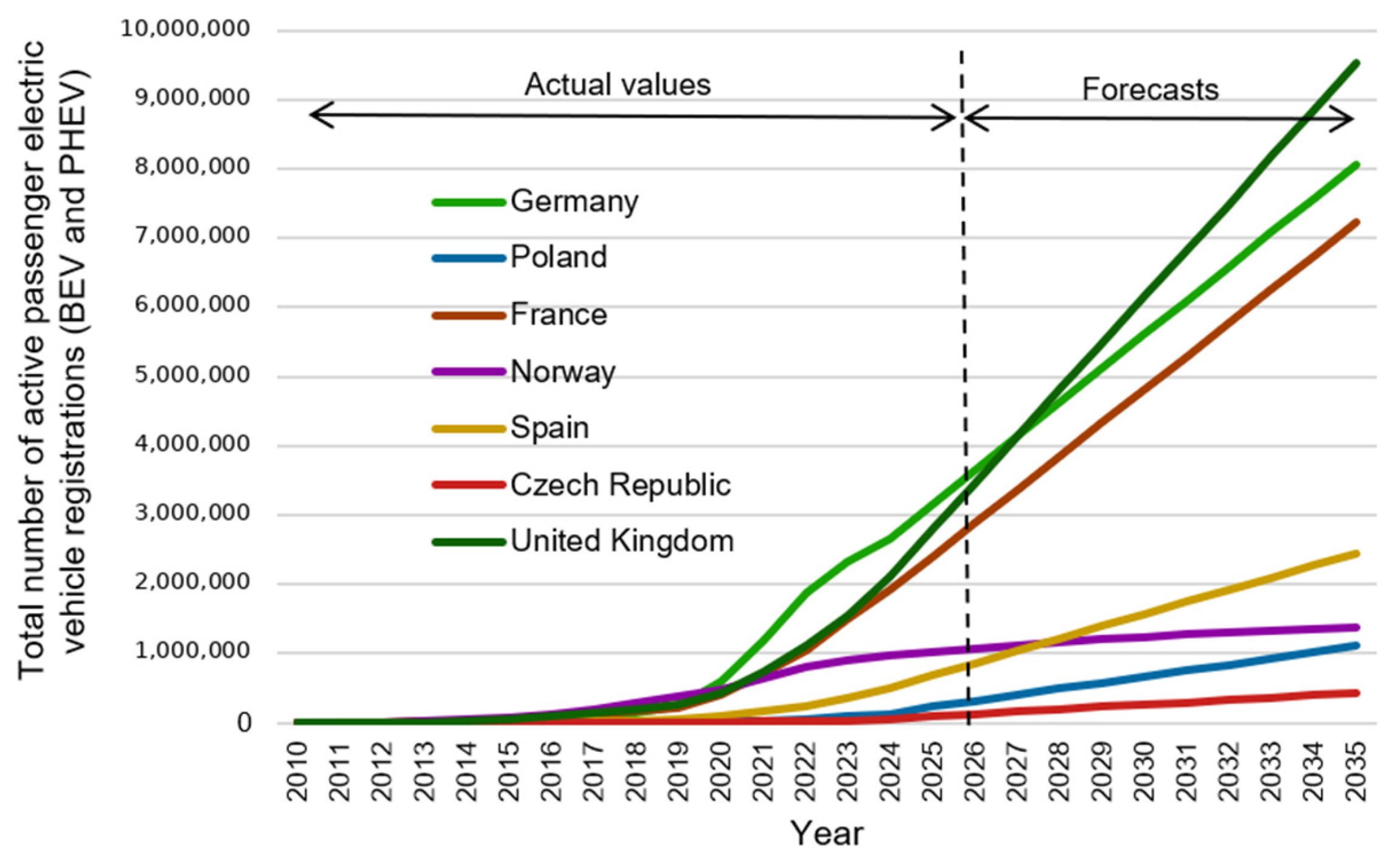
Damping allows the model to ‘decelerate’ growth, providing a better simulation of market saturation. This method introduces a damping parameter φ which causes the trend to converge toward a horizontal asymptote in the long-term horizon instead of increasing linearly. If φ = 1, the method is identical to the standard Holt’s method. Conversely, the smaller the φ parameter, the more pronounced the trend damping. The method optimizes model parameters with respect to the Sum of Squared Errors (SSE) using the Limited-memory Broyden–Fletcher–Goldfarb–Shanno with Box constraints (L-BFGS-B) algorithm. The DTES model was utilized to forecast the total number of active passenger electric vehicle registrations (BEV and PHEV) for the 2026–2035 period, based on historical data from 2010 to 2025 inclusive.
The model was applied independently using data from seven countries. Figure 7 depicts the actual values and the forecasts of the total number of active passenger electric vehicle registrations (BEV and PHEV) generated by the DTES model for the seven European countries under study. As a result of parameter optimization, optimal values were obtained that minimize the RMSE error over the historical data range. Regarding the damping parameter φ, it is noteworthy that a value of φ = 1 was achieved for six countries, with the exception of Norway, where φ = 0.9.

3.3. Modified Prigogine Logistic Model (MPL)

The modified Prigogine logistic equation is a discrete-time model based on deterministic chaos theory [26]. It describes the development of a population or a nonlinear system far from equilibrium, allowing for the observation of rapid demand increases, oscillations, bifurcations, and potential chaotic states. The model is used to describe the non-linear development of systems tending towards a state of saturation. It is a systemic model that incorporates a self-regulation mechanism; the model assumes that the growth rate is proportional to the current state of the system, while simultaneously being inhibited by the degree of saturation. The equation is defined as follows:
X t + 1 = X t [ 1 + R 1 X t K ]
where X t is the system state (e.g., number of adopters or demand) at time t, X t + 1 is the forecasted system state at time t + 1, R is the growth factor (speed of diffusion) and K is the carrying capacity (the asymptotic limit of the system’s development).
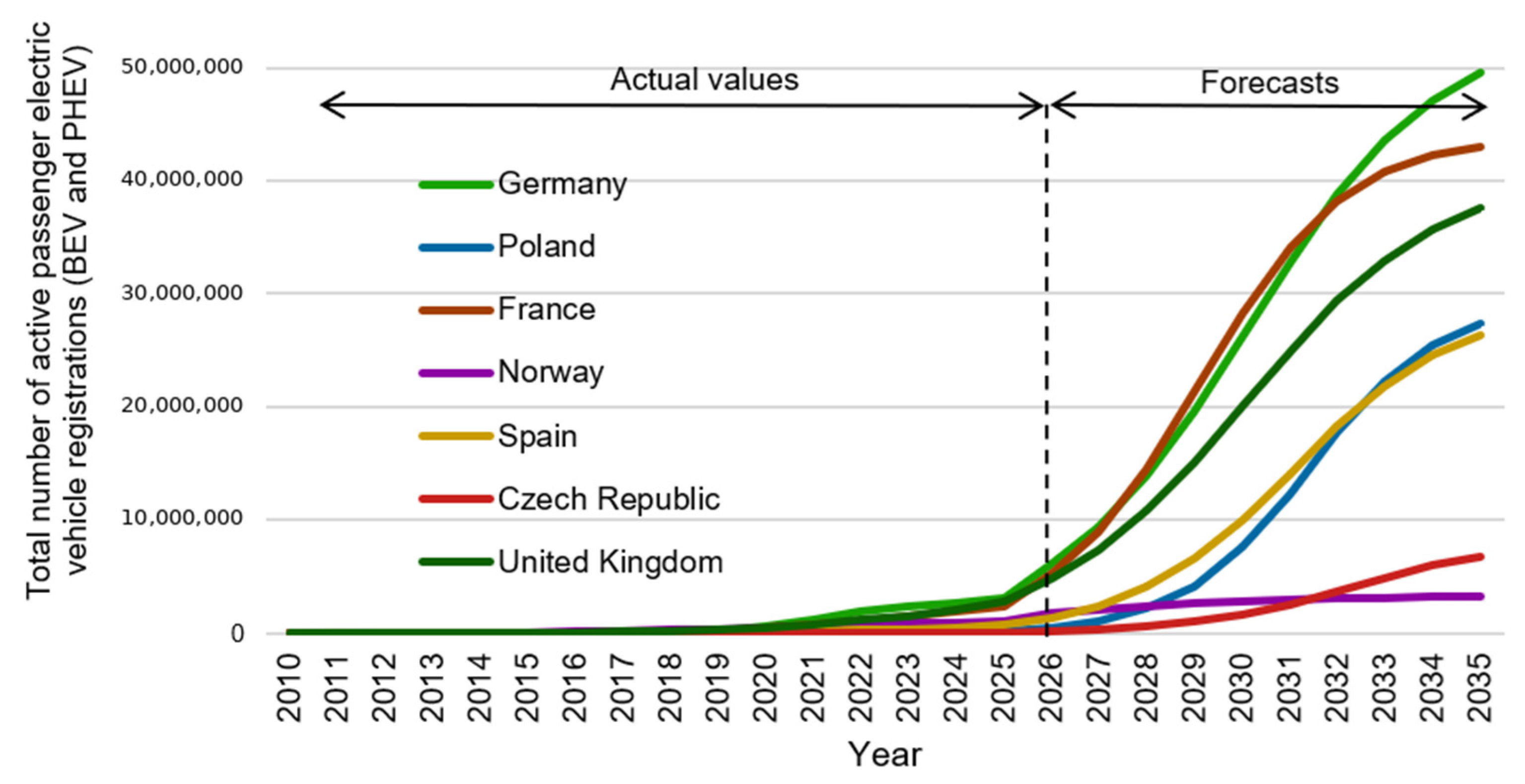
The primary advantage of the modified Prigogine model is its ability to capture complex, non-monotonic dynamic behaviors using a computationally simple structure. This makes it particularly useful for forecasting systems experiencing rapid, nonlinear technological shocks. However, its main disadvantage is extreme sensitivity to the growth parameter R and initial conditions.
The MPL model was used to forecast the total number of active passenger electric vehicle registrations (BEV and PHEV) for the 2026–2035 period, based on historical data from 2010 to 2025 inclusive. The model was applied independently using data from seven countries. Figure 8 depicts the actual values and the forecasts of the total number of active passenger electric vehicle registrations (BEV and PHEV) generated by the MPL model for the seven European countries under study. The L-BFGS-B algorithm was employed to optimize parameter R and K.

3.4. Continuous Logistic Model—Verhulst Equation (VLM)

The Continuous Logistic Model, introduced by Pierre François Verhulst, describes population growth or technological diffusion constrained by a carrying capacity. It results in a symmetric S-shaped (sigmoid) curve [27,28]. The differential equation and its explicit analytical solution are defined as follows:
N t = K 1 + ( K N 0 N 0 ) e r t
where N(t) is the cumulative number of adopters (or population size) at time t, r is the intrinsic growth rate, K is the carrying capacity (maximum market saturation limit) and N 0 is the initial population size or number of adopters at time t = 0.
The primary advantage of the continuous logistic model is its structural simplicity and the clear empirical interpretation of its parameters (growth rate and market capacity), which robustly models the entire life cycle of technology adoption. This model, much like the Modified Prigogine Logistic Model, features a physical interpretation of the saturation level. However, both models rely on a relatively rigid assumption regarding growth symmetry. The inflection point for both models occurs exactly at 0.5 K, and the terminal dynamics consist of a rapid convergence toward the value K.
The VLM model was used to forecast the total number of active passenger electric vehicle registrations (BEV and PHEV) for the 2026–2035 period, based on historical data from 2010 to 2025 inclusive. The model was applied independently using data from seven countries. Figure 9 depicts the actual values and the forecasts of the total number of active passenger electric vehicle registrations (BEV and PHEV) generated by the VLM model for the seven European countries under study. The L-BFGS-B algorithm was employed for model parameter optimization—r and K.

3.5. Grey Model (GM)

The basic Grey Model, known as GM(1,1), is derived from the grey system theory formulated by Julong Deng in 1982. It is a mathematical model designed for analysing systems with a “small sample and poor information,” where internal mechanisms are only partially known. The core idea of the model is to transform a chaotic time series into a series with an exponential structure through an accumulation operation, which allows for the application of differential equations. This model is more frequently applicable to the analysis of processes in less wealthy countries. Grey Model GM(1,1) is described by Equation (9) [29]. In this model, the order of the Grey Differential Equation and the number of variables are equal to 1. This model is recommended by Ref. [30], especially for very short time series and where the process evolution is in its initial phase.
y ^ ( t ) = y ^ ( 1 ) ( t ) y ^ ( 1 ) ( t 1 ) , y ^ ( 1 ) ( t ) = y ( 1 ) ( 1 ) u a · e ( a ( t 1 ) ) + u a y ^ ( 1 ) ( t ) = i = 1 t y ( i ) ,   t = 1,2 , , n
where n 4 is the length of time series, a is the evolution parameter, u is the grey variable and y ^ ( t ) is the forecast in period t.
The evolution parameter a determines the dynamics of the system’s changes. If a < 0 , the system grows; if a > 0 , the system exhibits a downward trend. The control constant (grey variable) u reflects the influence of external factors on the system (the so-called background).
The GM model was used to forecast the total number of active passenger electric vehicle registrations (BEV and PHEV) for the 2026–2035 period, based on historical data from 2010 to 2025 inclusive. The model was applied independently using data from seven countries. Figure 10 depicts the actual values and the forecasts of the total number of active passenger electric vehicle registrations (BEV and PHEV) generated by the GM model for the seven European countries under study. Three different optimizers were employed to optimize parameters a and u: L-BFGS-B, Nelder–Mead (a derivative-free simplex method), and Powell (a conjugate direction method). The latter exhibited the highest RMSE errors, and its results were consequently excluded from further analysis. For Poland, Spain, and the Czech Republic, the L-BFGS-B optimizer yielded the lowest RMSE values, while for the remaining four countries, the Nelder–Mead optimizer proved to be the most effective.

3.6. Bass Diffusion Model (BASS)

This model represents a benchmark in technology marketing and innovation diffusion analysis. Unlike the Verhulst model, the Bass Diffusion Model categorizes the population into two distinct groups: ‘Innovators’ (whose adoption is driven by external influences such as mass media) and ‘Imitators’ (whose adoption is driven by internal influences such as word-of-mouth). The Bass Diffusion Model is a widely utilized mathematical framework for forecasting the adoption of new products and technologies. The model is defined by the equation:
F t = M p ( 1 e p + q t ) p + q e p + q t
where N(t) is the cumulative number of adopters at time t, M is the market potential (the total number of potential adopters), p is the coefficient of innovation (external influence, such as advertising) and q is the coefficient of imitation (internal influence, such as word-of-mouth effects).
This model helps assess whether the growth of passenger electric vehicles (EVs) in a given country is being propelled by ‘early adopters’ (parameter p) or if the system has already transitioned into a phase of mass imitation (parameter q). In summary, the model elucidates the underlying cause of growth by distinguishing between external advertising and social interaction. However, a significant disadvantage is the assumption that the market potential (M) remains constant over time, which fails to account for market expansion, price fluctuations, or major policy shifts that frequently occur in the energy sector.
The BASS model was used to forecast the total number of active passenger electric vehicle registrations (BEV and PHEV) for the 2026–2035 period, based on historical data from 2010 to 2025 inclusive. The model was applied independently using data from seven countries. Figure 11 depicts the actual values and the forecasts of the total number of active passenger electric vehicle registrations (BEV and PHEV) generated by the BASS model for the seven European countries under study. Three different optimizers were employed to optimize parameters: M, p and q: L-BFGS-B, TNC (Truncated Newton), and SLSQP (Sequential Least Squares Programming). The latter optimizer, SLSQP, exhibited the highest RMSE values, and its results were consequently excluded from the analysis. For the United Kingdom, the TNC optimizer proved to be the most effective, while for the remaining six countries, the L-BFGS-B optimizer yielded the most favourable results.

3.7. Gompertz Growth Model (GOMP)

The Gompertz curve is a type of mathematical model for a time series, where growth is slowest at the start and end of a time period [31]. Unlike the logistic model, the Gompertz curve is characterized by an asymmetric sigmoid shape. The model is defined by the following equation.
N t = K · e a e b t
where N(t) is the cumulative number of adopters or population size at time t, K is the upper asymptote (market potential or carrying capacity), a is a constant related to the initial value of the series (displacement parameter) and b is the growth rate coefficient (determines the speed of diffusion).
The defining feature of the Gompertz model is its asymmetry, with the inflection point occurring relatively early in the diffusion process (at approximately 36.8% of the saturation level). This makes it highly advantageous for modeling technological adoptions that exhibit rapid initial growth followed by a long, slow maturation period. However, its primary disadvantage is the fixed position of the inflection point at 1/e, which may lack the flexibility required to fit empirical data where the peak growth occurs at different stages of the market life cycle.
The GOMP model was used to forecast the total number of active passenger electric vehicle registrations (BEV and PHEV) for the 2026–2035 period, based on historical data from 2010 to 2025 inclusive. The model was applied independently using data from seven countries. Figure 12 depicts the actual values and the forecasts of the total number of active passenger electric vehicle registrations (BEV and PHEV) generated by the GOMP model for the seven European countries under study. Three different optimizers were employed to optimize parameters K, a and b: L-BFGS-B, TNC, and SLSQP. The latter optimizer, SLSQP, exhibited the highest RMSE values, and its results were consequently excluded from the analysis. For Spain, the TNC optimizer proved to be the most effective, while for the remaining six countries, the L-BFGS-B optimizer yielded the most favourable results.

3.8. Multilayer Perceptron Neural Network as a Function Extrapolator (MLP)

The MLP model was used to forecast the total number of active passenger electric vehicle registrations (BEV and PHEV) for the 2026–2035 period, based on historical data from 2010 to 2025 inclusive. The model was applied independently using data from seven countries. MLP is typically utilized for regression (including forecasting [32]) and classification tasks [33], and it generally requires a large volume of training data. In this study, the MLP was first employed for nonlinear function approximation. In this context, there is no explicit analytical formula; instead, the mapping is embedded within the neural network’s architecture, its weights (parameters), and the activation functions of specific layers. Subsequently, the MLP was applied to extrapolate values beyond the training range [23].
The BFGS optimization algorithm was applied to optimize the weights (model parameters). Hyperparameter tuning was conducted to select the most appropriate models for each of the seven countries independently. The investigated number of hidden neurons ranged from 1 to 3, while the number of training epochs was evaluated for the values of 5, 10, and 20. The number of epochs had a significant impact on the ‘smoothness’ of the approximated function. Too many training epochs led to overfitting, causing the MLP to fit the historical observations too rigidly, thereby compromising its generalization capability. For the hidden layer, a hyperbolic tangent activation function was selected. In contrast, an exponential activation function was employed for the output layer—an unconventional yet deliberate choice, given the application of the MLP network to extrapolate functions characterized by exponential growth. Figure 13 depicts the actual values and the forecasts of the total number of active passenger electric vehicle registrations (BEV and PHEV) generated by the MLP model for the seven European countries under study.
The lowest RMSE was achieved for Germany, Poland, and the Czech Republic using an MLP architecture with a single neuron in the hidden layer. In turn, for France, Spain, Norway and the United Kingdom, the lowest RMSE was obtained with an MLP configuration featuring two hidden neurons.
It is worth noting that using an MLP model for a problem with a small number of samples is risky; however, a strong limitation on the number of training epochs, combined with the very small number of neurons tested in the hidden layer and the use of an exponential activation function in the output layer, provides justification for employing this model. A neural network constructed in this way has a very small number of weights (parameters). In the case of a single input and a single neuron, the model contains only one weight (the optimized parameter). The RMSE errors of this model were not extremely small for the seven forecasted countries over the weight-estimation period (2010–2025), which would otherwise suggest overfitting.

3.9. Ensemble Models

This subsection presents three different ensemble models utilizing the results of the previously described single-model forecasts (Phase 3). The analysis of RMSE values over the validation horizon (2022–2025), conducted for each model and by country, indicated that, according to expert assessment, none of the single-model specifications yielded RMSE errors sufficiently large to justify model rejection. The trimming procedure was introduced to improve the robustness of long-horizon ensemble forecasts. To mitigate the risk of model-specific instabilities—particularly evident in non-linear logistic growth models and neural networks when extrapolated—the extreme minimum and maximum 2035 forecasts were excluded for each country. This procedure ensures that the final ensemble (SAE, G-IRWE, L-IRWE) is not skewed by outlier trajectories, focusing instead on the consensus of the best-performing models. Table 3 summarizes the forecasted values for active passenger EV registrations (BEV and PHEV) in 2035. The two models rejected for each country are indicated in red with a strikethrough. Consequently, in the subsequent step, only five selected single models were used to construct the ensemble models for each country. This procedure ensured that the least realistic forecasts, acting as outliers, were not incorporated into the ensemble models. In summary, the exclusion procedure applied before ensemble construction was based on the extremeness of the 2035 forecast values, not directly on RMSE. For each country, the single model producing the lowest 2035 forecast and the single model producing the highest 2035 forecast were removed. This trimming step was introduced to reduce the influence of potentially unstable long-term extrapolations on the ensemble forecasts. RMSE values were then used only in the weighting procedures of the G-IRWE and L-IRWE ensembles for the five retained models. Therefore, Table 3 reports the 2035 forecast values used for identifying extreme projections, while Table 4 and Table 5 report the RMSE and RMSE5 values used in the subsequent weighting procedures.
The excluded models are not interpreted as universally invalid; rather, their 2035 projections were treated as country-specific outliers relative to the remaining model pool.

3.9.1. Simple Averaging Ensemble (SAE)

The Simple Averaging Ensemble is described by Equation (12). The final forecast within this ensemble is calculated as the arithmetic mean of the projections from five out of the seven models (under the assumption of discarding the two extreme models—specifically, those yielding the highest and lowest forecast values for the year 2035). Averaging the predictive results across diverse models is intended to enhance the overall reliability of the forecasting [12].
y ^ t = 1 k i = 1 k y ^ t i
where y ^ t is the final ensemble forecast for time t, k is the total number of individual models included in the ensemble, y ^ t i is the forecast generated by the i-th individual model for time t, and i is the index of the specific model (i = 1, 2,…, k).
The primary advantage of this approach is the reduction in the variance of the forecast error and the mitigation of the risk associated with selecting a single, poorly performing model (the “wisdom of the crowd” effect). It is computationally efficient and prevents overfitting by smoothing out the idiosyncratic biases of individual methods. However, its main disadvantage is that it treats all models as equally reliable, potentially lowering the overall accuracy if one of the constituent models is significantly less precise than the others.
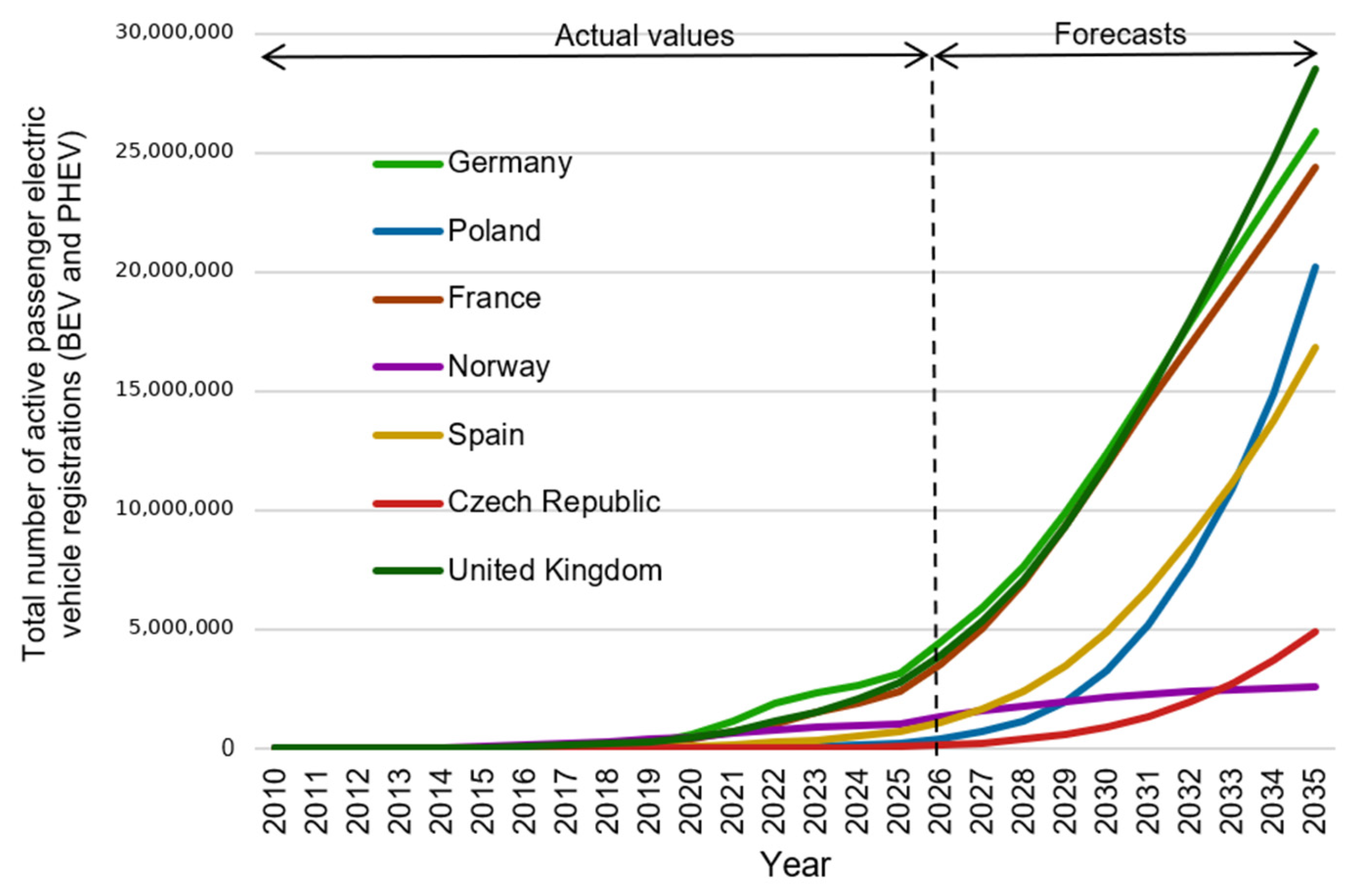
In the construction of the SAE model using five single models, each model is assigned an equal weight of 0.2 within the ensemble. Figure 14 depicts the actual values and the forecasts of the total number of active passenger electric vehicle registrations (BEV and PHEV) generated by the SAE model for the seven European countries under study.

3.9.2. Global Inverse RMSE-Weighted Ensemble (G-IRWE)

The forecast of the weighted ensemble model at time t is defined as the convex combination of the individual forecasts, where the sum of all weights equals exactly 1 [34]. The model is defined by the following equation.
y ^ t = i = 1 k w i y ^ t i
where y ^ t is the final ensemble forecast for time t, k is the total number of individual models included in the ensemble, y ^ t i is the forecast generated by the i-th individual model for time t and w i is the weight assigned to the i-th model, subject to the constraint i = 1 k w i = 1 .
In this variant (G-IRWE), the weights are inversely proportional to the Root Mean Square Error (RMSE) calculated over the entire available historical dataset. This approach favors models with long-term global stability. The weight for the i-th model is calculated as follows:
w i = 1 R M S E i j = 1 k 1 R M S E j
where R M S E i is Root Mean Square Error of the i-th model calculated over the entire historical in-sample period.
The G-IRWE model was developed utilizing the five previously selected single models. The weight of each single model was calculated according to Equation (14). Table 4 provides a comprehensive summary of the RMSE values calculated across the entire historical period (2010–2025) for each of the seven countries and the five selected single models (following the prior exclusion of the two models generating extreme 2035 forecasts—see Table 2).
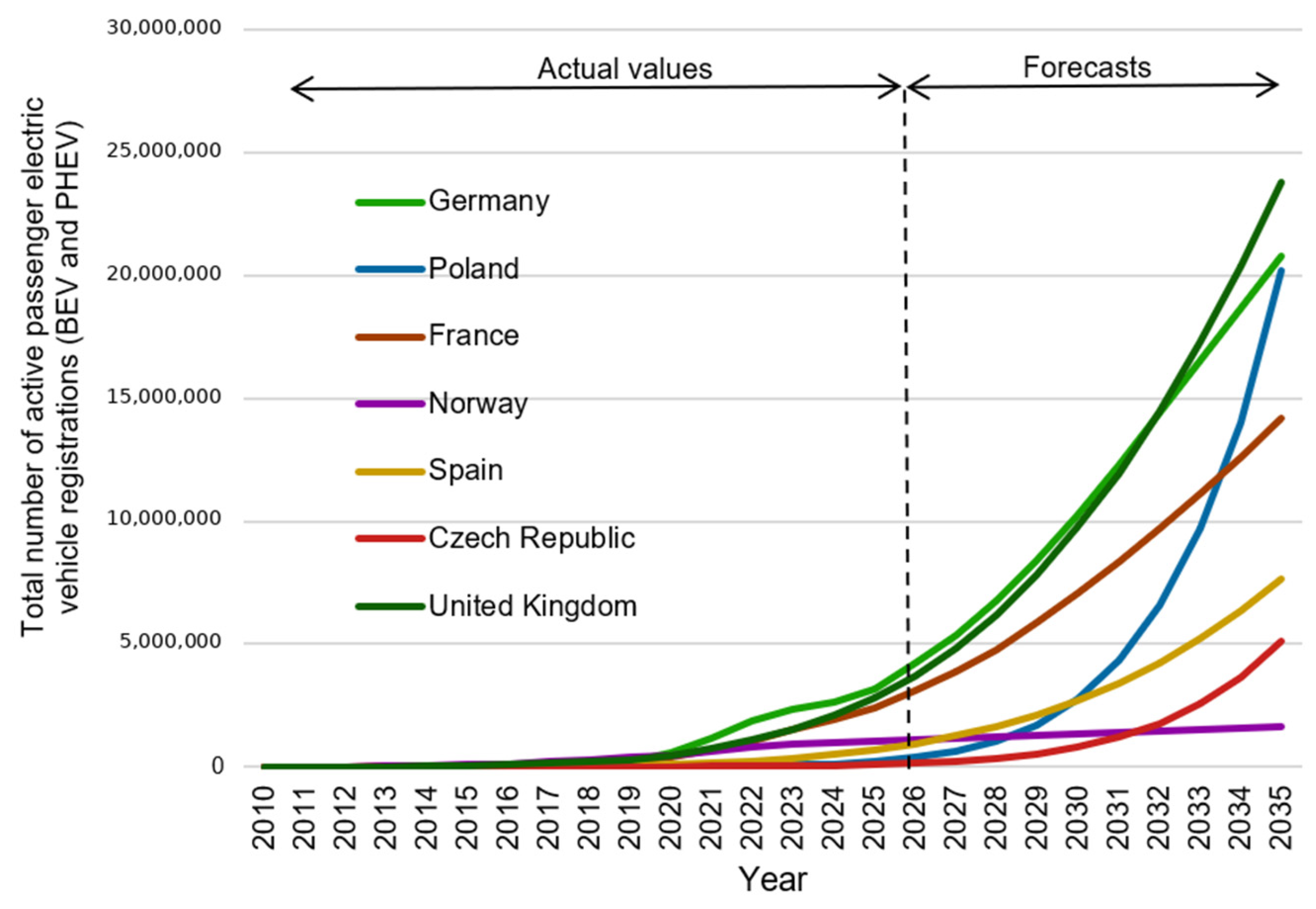
Figure 15 depicts the actual values and the forecasts of the total number of active passenger electric vehicle registrations (BEV and PHEV) generated by the G-IRWE model for the seven European countries under study.

3.9.3. Local Inverse RMSE-Weighted Ensemble (L-IRWE)

In this variant of the weighted ensemble model (L-IRWE), the weights are dynamically adjusted based on the models’ performance in the most recent periods. The weights are inversely proportional to RMSE5, calculated solely from the last five historical observations. This approach favors models that quickly adapt to recent structural changes or local trends. However, the main limitation of this approach is that assigning model weights based on a short error-estimation window (N = 5), while targeting a 10-year forecasting horizon (through 2035), makes the procedure sensitive to random end-of-sample noise. This, in turn, undermines the asymptotic stability of the resulting forecast. Nevertheless, the model was deemed worth applying and was subsequently benchmarked against alternative results. The weight for the i-th model is calculated as follows:
w 5 , i = 1 R M S E 5 , i j = 1 k 1 R M S E 5 , j
where R M S E 5 , i is Root Mean Square Error of the i-th model calculated strictly over the window of the five most recent historical observations prior to the forecast origin and w 5 , i is weight assigned to the i-th model based on its recent performance.
The L-IRWE model was developed utilizing the five previously selected single models. The weight of each single model was calculated according to Equation (15). Table 5 provides a comprehensive summary of the RMSE5 values, calculated exclusively based on historical data from the final five years of the known period (2021–2025), for each of the seven countries and the five selected single models (following the prior exclusion of the two models generating extreme 2035 forecasts—see Table 2).
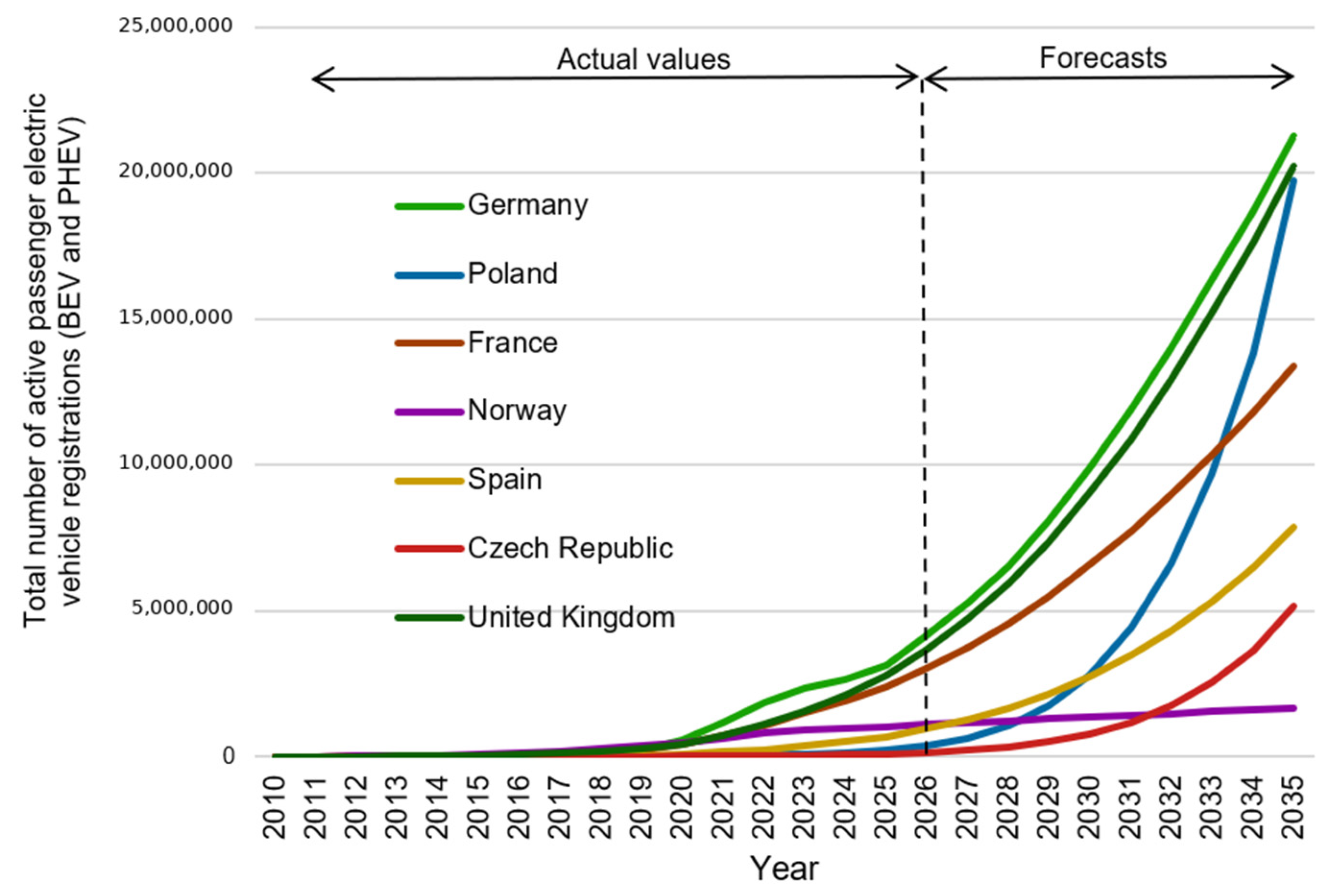
Figure 16 depicts the actual values and the forecasts of the total number of active passenger electric vehicle registrations (BEV and PHEV) generated by the L-IRWE model for the seven European countries under study.
It is worth emphasising that the L-IRWE variant should therefore be interpreted as a sensitivity-oriented ensemble rather than as a universally superior weighting scheme. Its advantage is that it can react to recent structural changes in the EV market, which may be relevant in a rapidly evolving sector. However, because the weighting window contains only five observations, it may also amplify random end-of-sample fluctuations. For this reason, the L-IRWE results are interpreted jointly with the SAE and G-IRWE results. In particular, when L-IRWE-based forecasts diverge substantially from the other ensemble projections, the corresponding long-term forecast should be treated with increased caution.
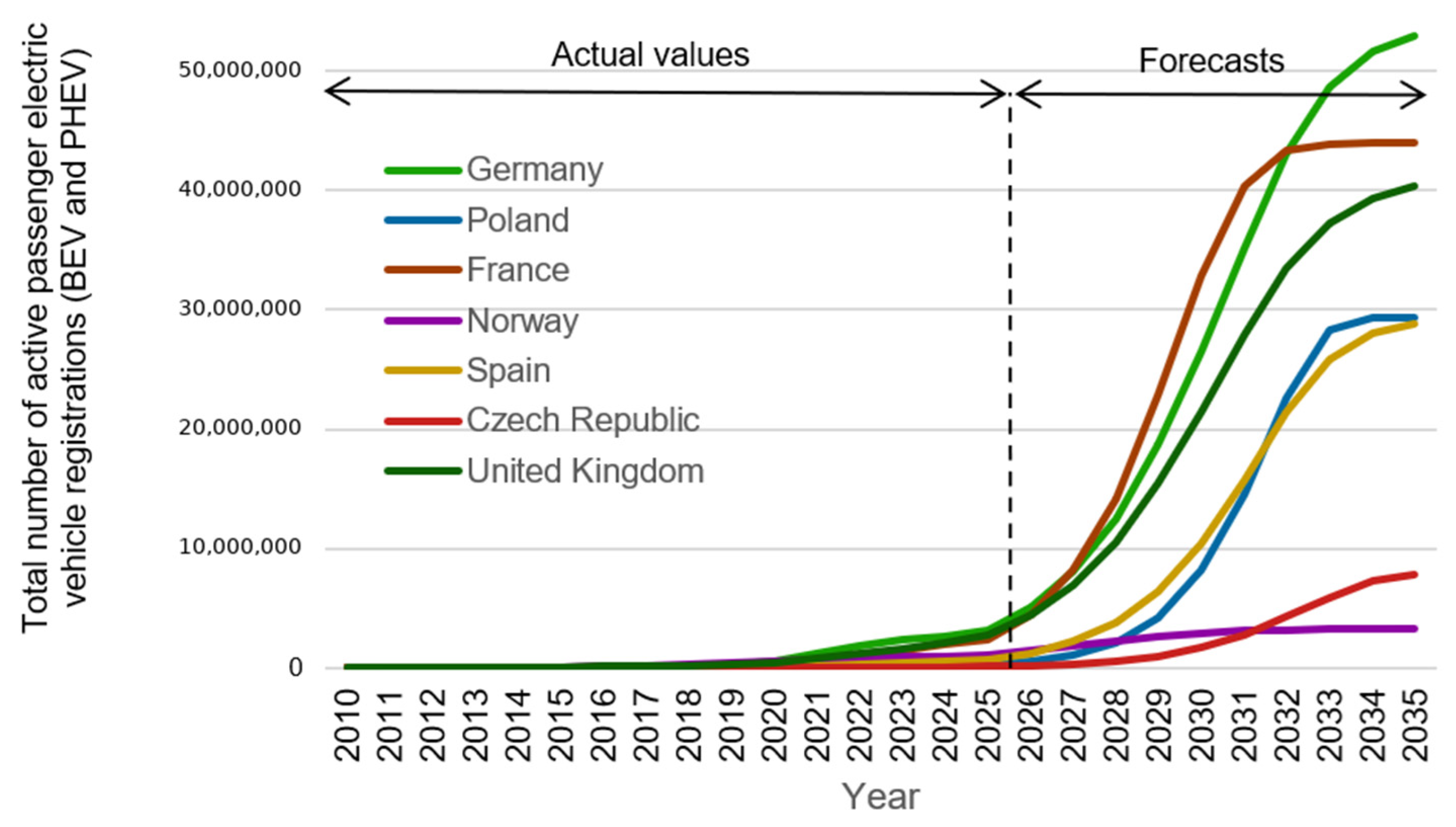
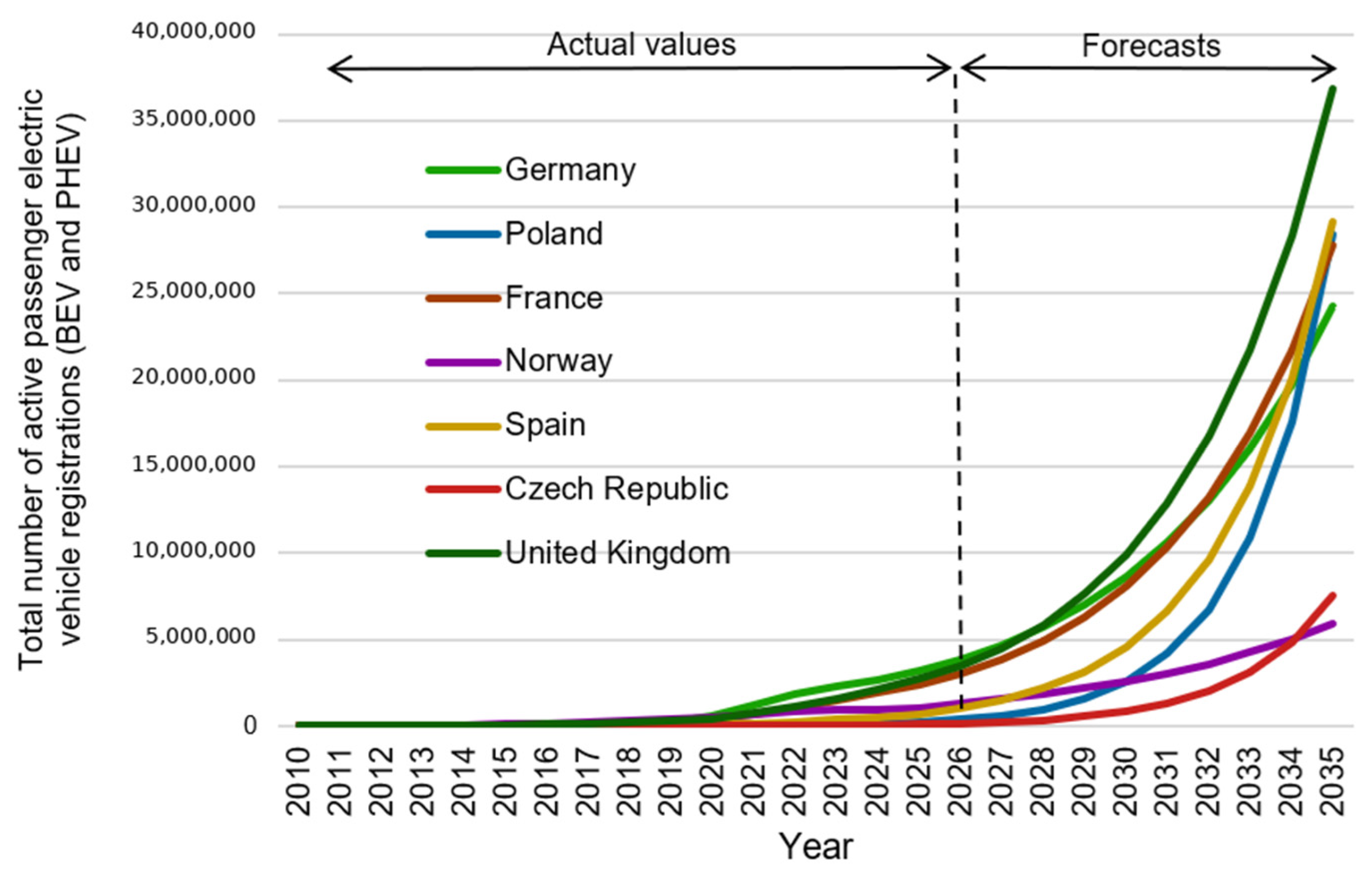
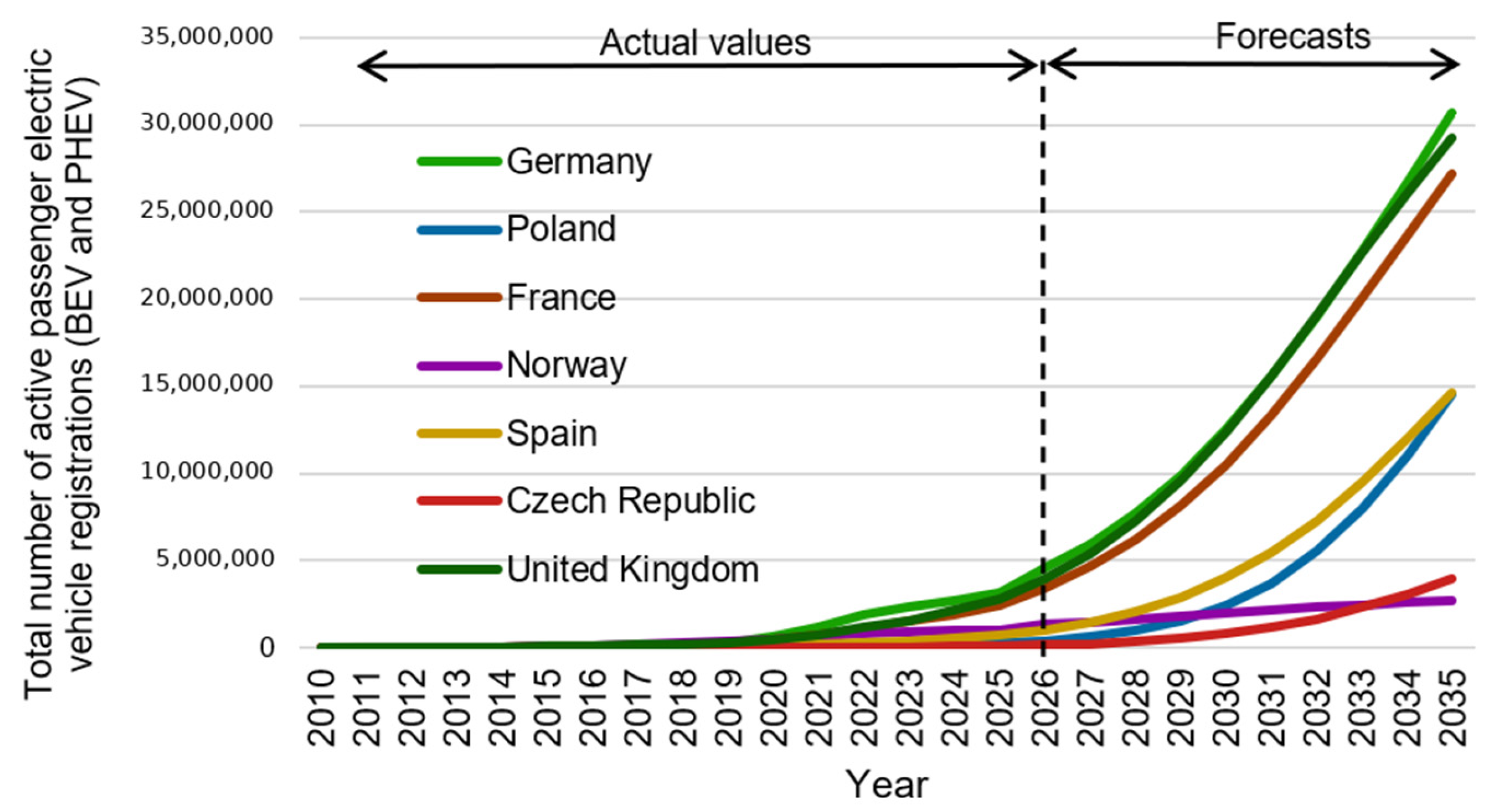
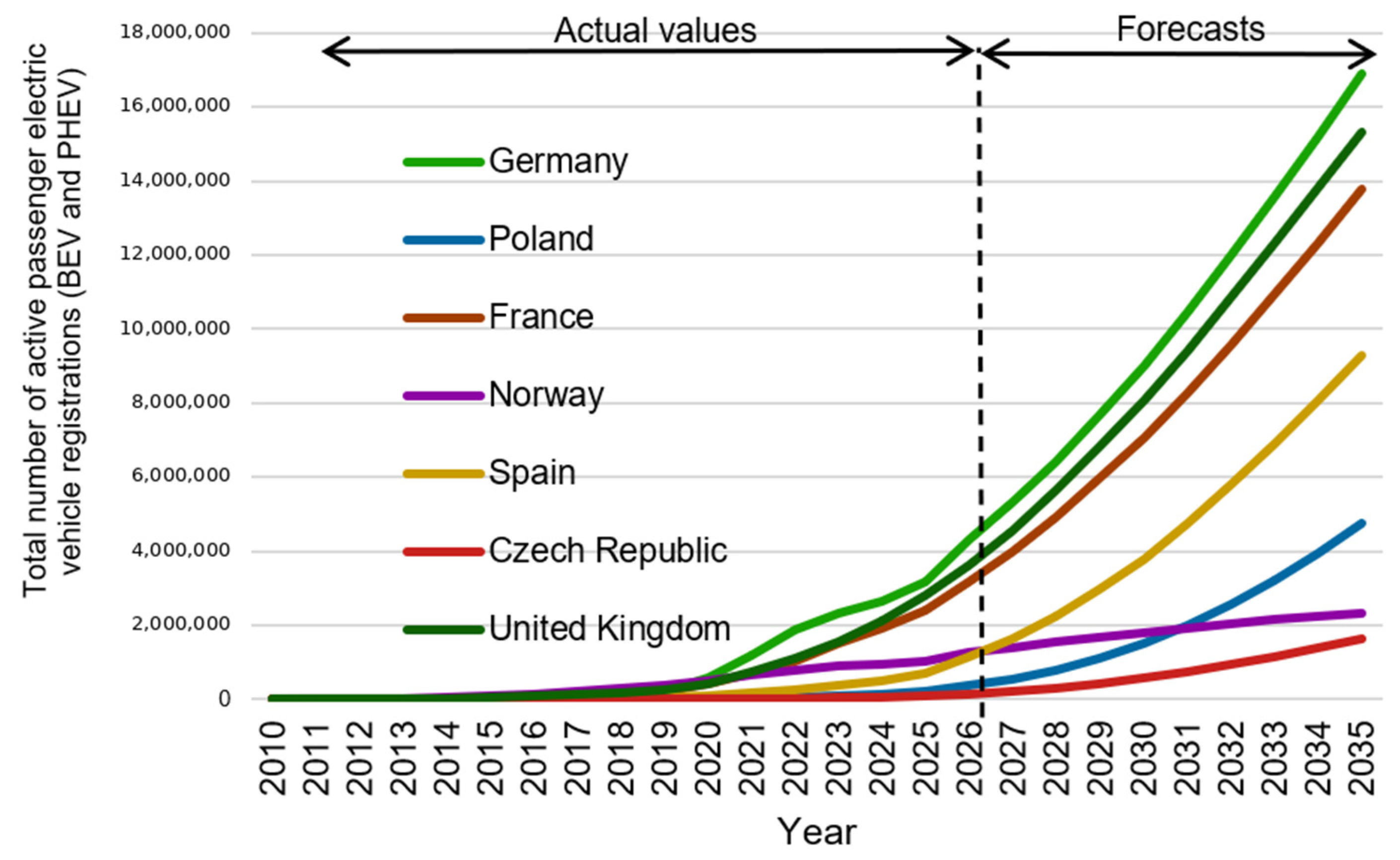
In the next step (Phase 4), three forecast ensemble projections were selected for each of the seven countries based on the results of the three ensemble models (SAE, G-IRWE, and L-IRWE). The low ensemble projection is defined as the ensemble model yielding the lowest 2035 forecast value, while the high ensemble projection corresponds to the model with the highest 2035 forecast value. The middle ensemble projection represents the ensemble model with the intermediate (non-extreme) 2035 forecast value. Table 6 presents the results of this ensemble projections selection for each country, derived from the 2035 projections of the three ensemble models.
The three ensemble projections may be interpreted as trend-based counterparts of conservative, central, and optimistic variants. However, they should not be understood as full policy scenarios in the strict sense, because no explicit assumptions are imposed regarding future electricity prices, charging-infrastructure costs, subsidy schemes, vehicle prices, income growth, or regulatory changes. Instead, the low, middle, and high projections reflect the range of outcomes generated by alternative ensemble-weighting mechanisms applied to the same historical EV time series. Thus, the projection framework captures methodological uncertainty, while externally defined scenario analysis remains a natural extension for future research.
The low, middle, and high projections should not be interpreted as probability-based scenarios or confidence intervals. They are model-based projection variants obtained from the three ensemble methods. For each country, the lowest, intermediate, and highest 2035 ensemble forecasts were labelled as low, middle, and high projections, respectively. Thus, the projection range reflects methodological uncertainty associated with alternative ensemble constructions rather than probabilistic uncertainty or explicitly defined policy pathways.
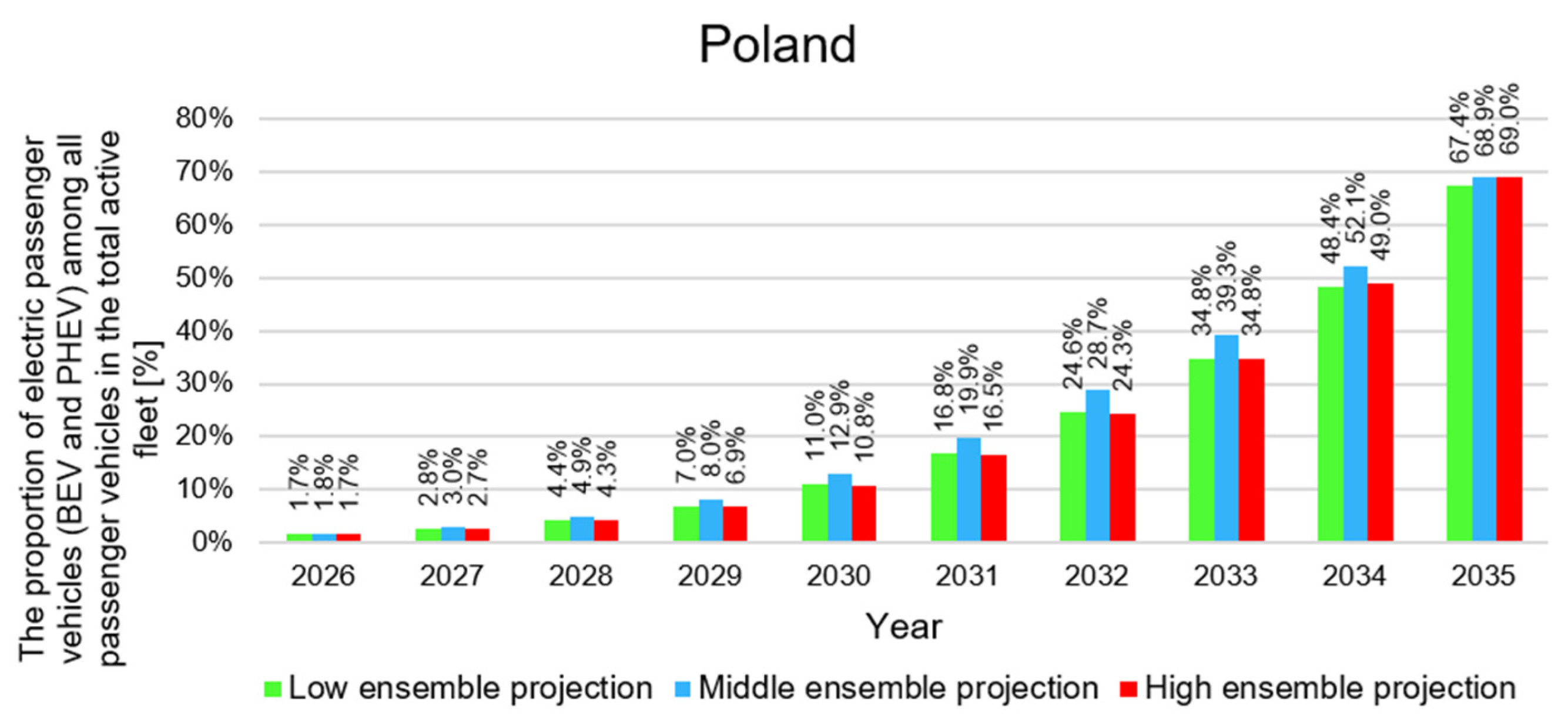
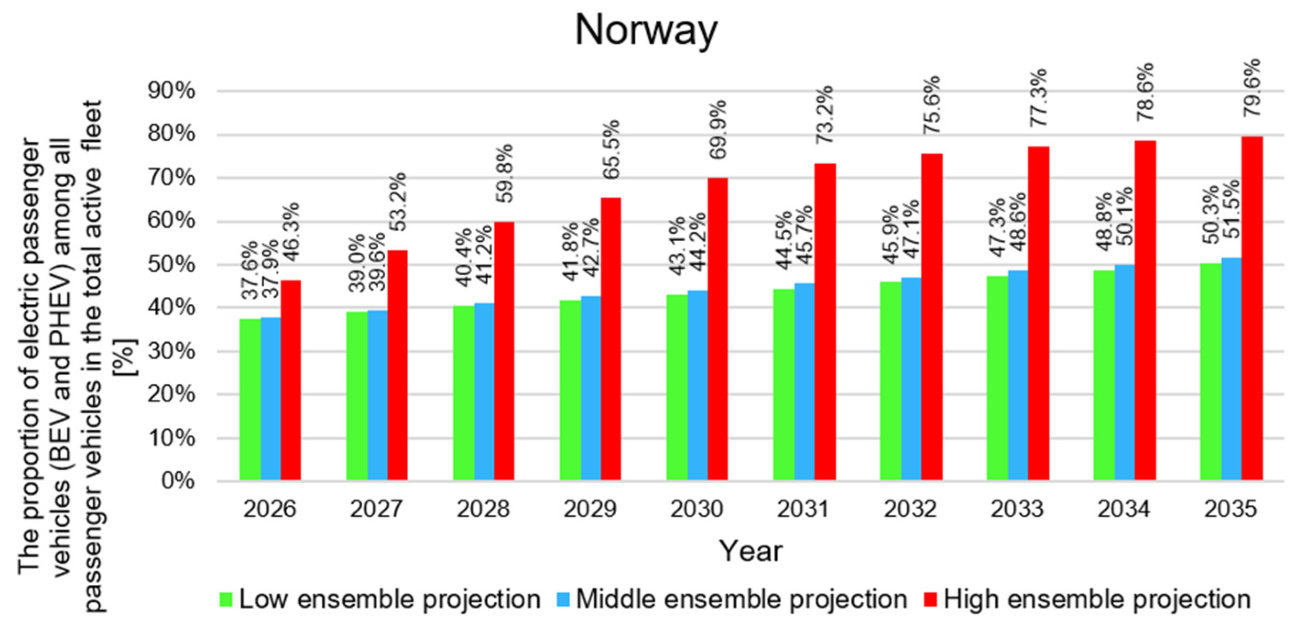
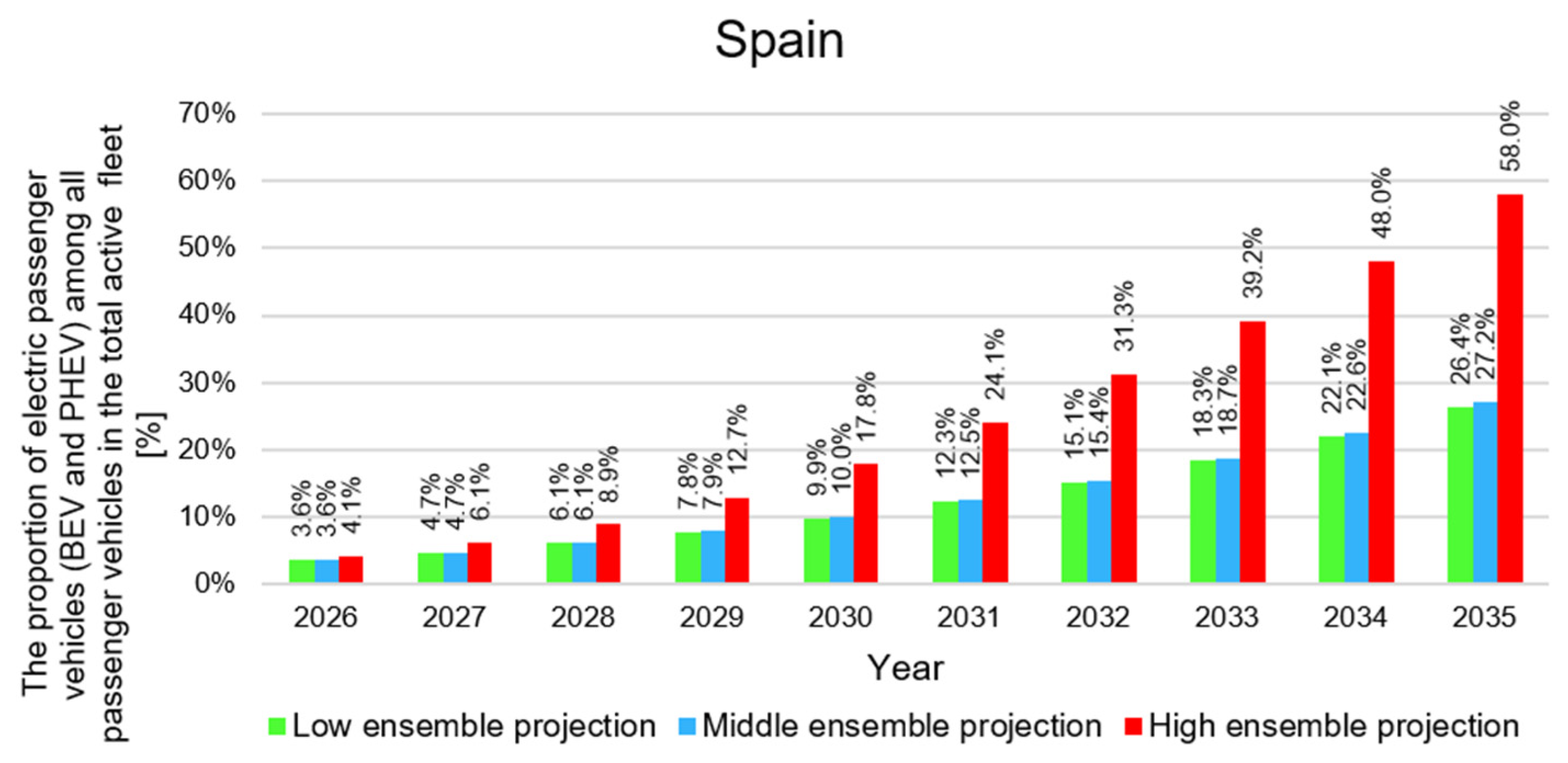
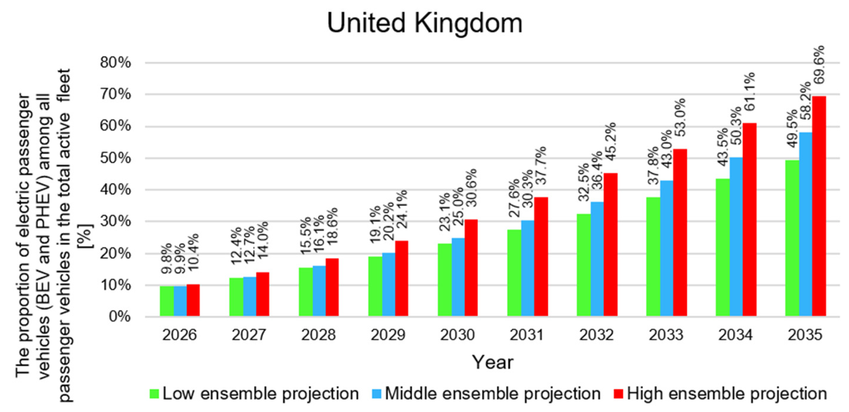
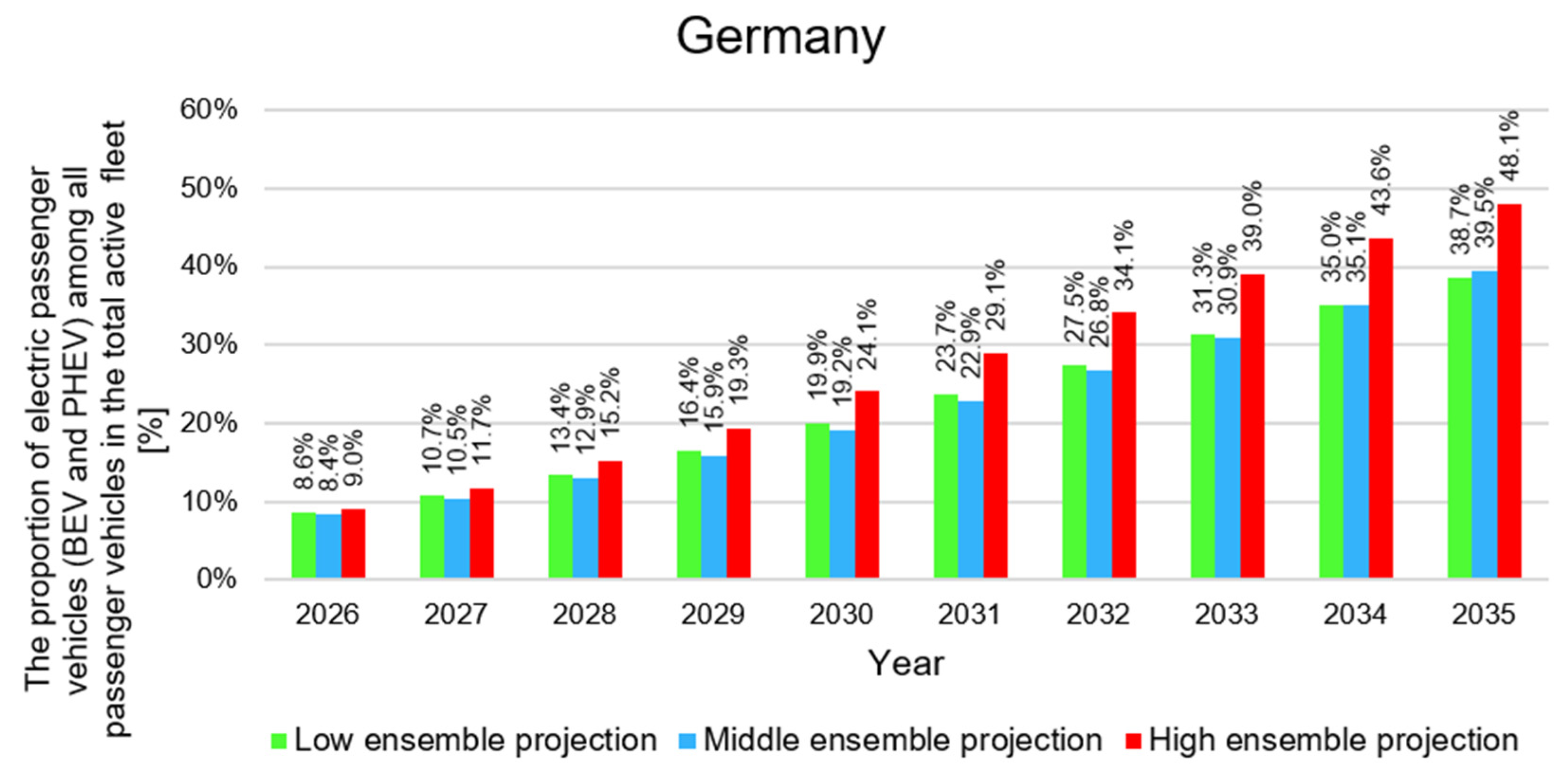
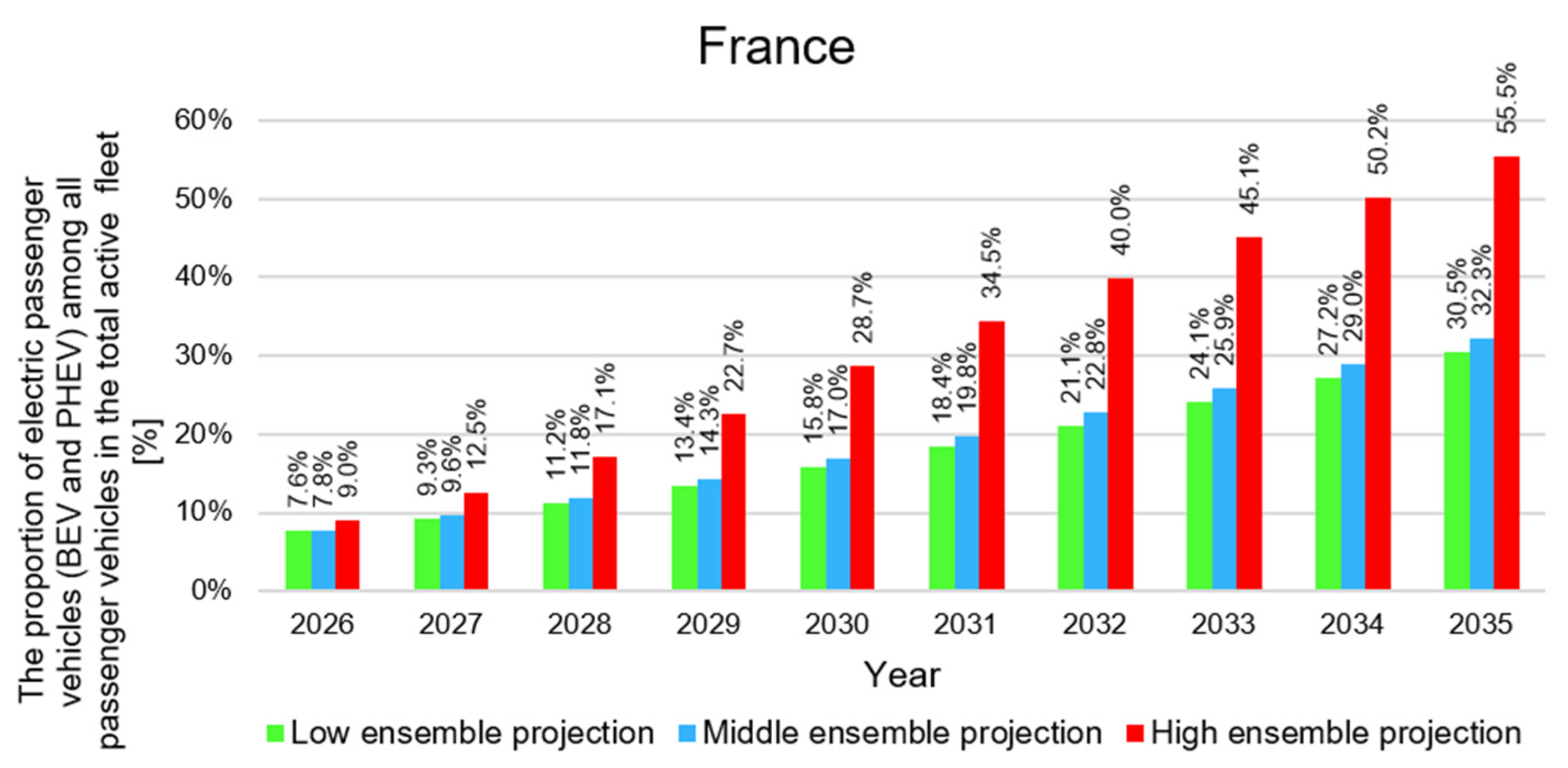
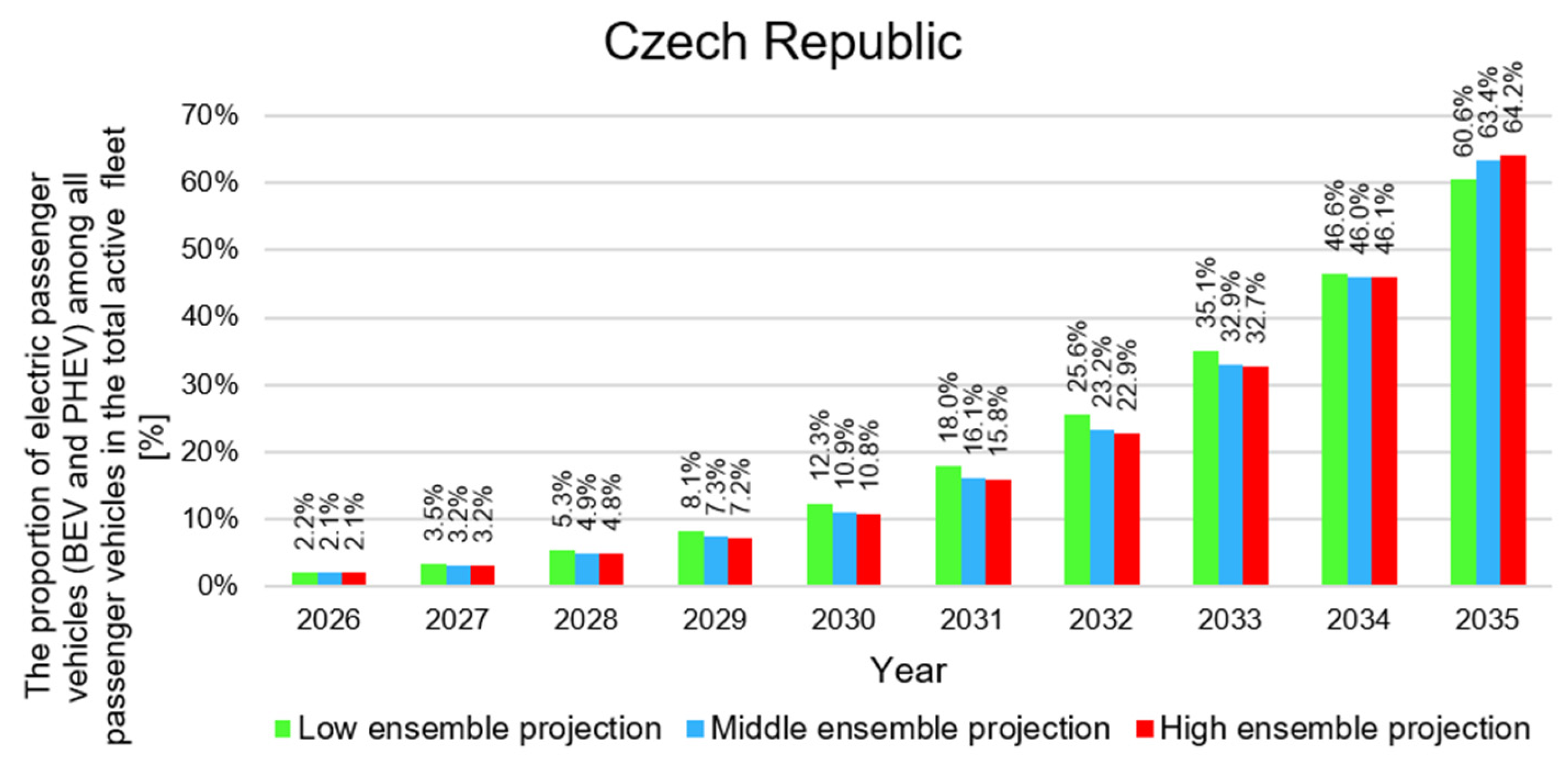
In the final step (Phase 5), the EV (BEV and PHEV) share of the total active passenger vehicle registrations for each of the seven countries (2026–2035) was determined. These calculations were based on the results from the ensemble models for the three ensemble projections and the forecast results (2026–2035) for the total number of passenger vehicle registrations across all drivetrain types. Figure 17, Figure 18, Figure 19, Figure 20, Figure 21, Figure 22 and Figure 23 illustrate the final results of the study, namely the three-projection forecasts for the 2026–2035 period across the seven analysed countries.

4. Discussion

4.1. Analysis and Interpretation of Projection Results

The statistical analysis conducted prior to the forecasting stage—based on three different normalization approaches—provided an alternative perspective on the development of electromobility across the seven analysed countries. Nevertheless, the most informative results were obtained from Min–Max normalization, which, for example, revealed a clear separation of the analysed countries into three groups according to the level of electromobility development. An analogous outcome was obtained by calculating the percentage share of active registered electric passenger vehicles (BEVs and PHEVs) within the total passenger-car fleet, irrespective of powertrain type.
Single-model forecasts were produced using seven models, two of which incorporated a development ceiling (MPL and VLM). This provided a broader view of the prospective evolution of electromobility in the passenger-car segment. Among the analysed single forecasting models, DTES and MPL performed least favourably (i.e., they generated the largest number of outlying forecasts relative to the remaining models across the seven countries). In contrast, the VLM, BASS, and GOMP models merit particular attention: for none of the seven countries did forecasts produced by these models constitute extreme projections (i.e., candidates for exclusion in ensemble forecasting). It is worth noting that the GM model—recommended for the early phase of process development—was rejected in the case of Norway, which is logically consistent given Norway’s highest level of electromobility development. Another noteworthy observation is that the same two models (DTES and MLP) were rejected for the three countries characterised by a low level of electromobility development (Poland, Czech Republic, and Spain).
An analysis of preferred-model selection among the three ensemble models across three development ensemble projections showed that, under the low ensemble projection, no single ensemble model dominated across the seven analysed countries. A similar pattern was observed for the middle ensemble projection. By contrast, under the high ensemble projection, the SAE model was selected most frequently (five selections). Importantly, SAE was chosen almost exclusively for countries with a high level of electromobility development (Germany, France, Norway, and the United Kingdom). Spain constituted the exception, as SAE was also selected for this country. Overall (21 ensemble-model selections), no model dominated the others: each of the ensemble models—SAE, G-IRWE, and L-IRWE—was selected seven times.
When analysing the final results for the share of total active passenger vehicle registrations in each of the seven countries (2026–2035), it can be observed that there are substantial cross-country differences, both in the achieved percentage levels and in the magnitude of ensemble projection-related variation within a given country. For Germany, the conservative and middle ensemble projections are nearly identical, whereas the high ensemble projection is more than 8 percentage points higher. A markedly different pattern is observed for Poland, where all three ensemble projections yield almost identical results in 2035, which may indicate increased forecast robustness for this country. A similar convergence of ensemble projection outcomes is also found for the Czech Republic; both countries share a relatively low level of electromobility development in 2025. In the case of the United Kingdom, the three ensemble projections diverge in 2035, but only to a limited extent—these results appear typical for an ensemble projection-based forecasting framework. By contrast, France, Norway, and Spain exhibit a comparable pattern of differentiation across ensemble projections, with conservative and balanced results being very close, and the high ensemble projection producing nearly double the values. Such strongly divergent outcomes may be regarded as outliers relative to the other two ensemble projections and, consequently, as the least credible.
When, in turn, analysing the share of total active passenger vehicle registrations (2026–2035) in terms of electromobility growth dynamics between 2025 and 2035—focusing on the middle ensemble projection—the country-specific trajectories remain heterogeneous. Table 7 summarizes the stages of electromobility development starting from the end of 2026 (a 1-year-ahead forecast), through the end of 2030 (a 5-year forecast horizon), and up to the end of 2035 (a 10-year forecast horizon).
The analysis of the forecast results presented in Table 6 indicates that the largest percentage increase in electromobility is projected for Poland, Czech Republic, and the United Kingdom, whereas the smallest increase is projected for Germany and Spain. The result for Norway is notable, as it suggests a transition into the saturation phase of the process. In terms of development dynamics—comparing the forecasts for 2026 and 2035—the largest change is observed for Poland and Czech Republic. The smallest dynamics of change occur in Norway. For Germany and France, the growth dynamics are considerably lower than, for example, in the Czech Republic and Poland.
The interpretation of country-specific forecasts should also take into account jurisdiction-specific regulatory and policy contexts. Norway represents a mature EV market in which adoption has been strongly supported by long-standing fiscal incentives, taxation rules favouring zero-emission vehicles, and a national objective for new passenger cars to be zero-emission. The United Kingdom is influenced by the ZEV mandate, which sets binding annual targets for the share of new zero-emission cars and vans. The EU Member States analysed in this study are subject to common EU-level CO2 standards for new cars and vans and to the Alternative Fuels Infrastructure Regulation, but national implementation conditions, purchasing power, charging-infrastructure availability, electricity prices, and fiscal incentives differ substantially. These differences may explain why countries with similar historical EV-stock growth may diverge in future observations. The Polish case additionally requires caution because the 2024 statistical decline in the total passenger-vehicle fleet resulted from an administrative clean-up of inactive registrations rather than from an actual physical reduction in the active vehicle stock.
The proposed approach can be compared with several related forecasting strategies used in EV-market and technology-diffusion studies. Single-model approaches, such as logistic, Gompertz, Bass, grey, exponential-smoothing, and ARIMA/SARIMA, usually require the analyst to select one preferred specification. By contrast, the present method first generates forecasts from several structurally different models and then constructs trimmed ensembles after excluding the lowest and highest 2035 projections. This procedure reduces dependence on any single model and limits the impact of unstable extrapolations. Compared with standard equal-weight ensembles, the G-IRWE and L-IRWE variants additionally incorporate information on historical forecasting errors through inverse-RMSE weighting. Compared with more data-intensive machine-learning or multivariate econometric methods, the proposed framework is better suited to very short annual time series, but it does not explicitly model exogenous drivers. Therefore, its main contribution lies in providing a transparent and robust trend-based ensemble procedure for small-sample long-horizon EV-stock forecasting. Table 8 shows a conceptual comparison of the proposed method with related forecasting approaches.
The proposed method has several advantages and limitations. Its main advantage is that it is transparent and applicable under severe data constraints, especially when only short annual EV-stock time series are available. By combining structurally different models and excluding the two most extreme 2035 projections before ensemble construction, the approach reduces dependence on a single model specification and limits the influence of unstable long-term extrapolations. The use of three ensemble variants also makes it possible to assess the sensitivity of results to alternative weighting assumptions. At the same time, the method remains trend-based and univariate. It does not explicitly incorporate explanatory variables such as energy prices, charging-infrastructure availability and costs, EV purchase prices, subsidy schemes, taxation, household income, or restrictions on new internal combustion engine vehicle sales. These factors may substantially affect future EV adoption, especially over a 10-year horizon. Consequently, the forecasts should be interpreted as conditional projections based on historical EV-stock dynamics rather than as full policy or market scenarios.
The method does not impose an explicit assumption that the number of BEVs and PHEVs must grow faster than the total passenger-vehicle fleet. The EV stock and the total passenger-vehicle stock are forecast separately, and the projected EV share is obtained only in the final step as their ratio. Nevertheless, because the historical EV-stock trajectories grow much faster than the total vehicle-stock trajectories, this difference is naturally reflected in the extrapolated results. The framework therefore captures the continuation of historical growth dynamics, but it does not explicitly simulate future restrictions on new ICE vehicle sales, EV purchase incentives, taxation changes, or other policy instruments.
A limitation of trimming is that it reduces the range of model-generated uncertainty. Therefore, the trimmed ensembles should be interpreted as robust central projection variants rather than as a full representation of all possible model outcomes. Future work could compare trimmed and untrimmed ensembles explicitly as an additional sensitivity test.

4.2. Policy Implications of the Projection Variants

The low, middle, and high projections are not probability-based scenarios, but they can still inform policy discussion. They indicate the range of EV-stock shares that may result if historical adoption dynamics continue under alternative ensemble assumptions. From a policy perspective, the low projection may be interpreted as a warning that current adoption dynamics may be insufficient to meet long-term decarbonisation expectations. The middle projection represents the most balanced trend-based outcome and may be the most useful for infrastructure planning. The high projection indicates the level of pressure that could arise on charging infrastructure, distribution grids, parking facilities, and public support schemes if EV adoption accelerates strongly.
For countries with currently low EV shares, such as Poland and the Czech Republic, even a moderate continuation of recent growth could imply a rapid increase in infrastructure needs. This would require accelerated deployment of public and residential charging, distribution-grid reinforcement, and stable regulatory incentives. For medium-development countries such as Germany, France, Spain, and the United Kingdom, the main policy challenge is to align EV uptake with charging-network expansion, electricity-system readiness, and affordability. In the United Kingdom, this is particularly relevant because the ZEV mandate creates a binding regulatory pathway for new zero-emission vehicle sales. For Norway, where EV adoption is already advanced, the policy challenge is less about initiating adoption and more about managing a mature EV system, including charging reliability, grid integration, incentive redesign, and the transition from purchase stimulation to efficient system operation.
These implications should be interpreted cautiously. The projections do not directly model future policy interventions, energy-price shocks, subsidy changes, or infrastructure bottlenecks. They therefore indicate potential planning pressures under trend continuation rather than providing a complete policy-scenario assessment.


5. Conclusions

The final results obtained from the ensemble models are, admittedly, somewhat surprising. However, it should be emphasized that the models applied in this study rely exclusively on information contained in the time series of the forecasted process itself. From this perspective, it appears, first, that the forecasts generated by the ensemble models under the middle ensemble projection are the most credible and, second, that these forecasts appear realistic for the 5-year horizon (up to the end of 2030).
In the case of forecasts with a 10-year horizon (up to the end of 2035), the degree of uncertainty increases. The 2035 projections should not be interpreted as deterministic point forecasts. Rather, they represent conditional trend-based extrapolations derived from the historical EV-registration trajectories observed in 2010–2025. Some of the long-term outcomes, especially where the high projection diverges strongly from the low and middle projections, should therefore be treated as indicators of model-based uncertainty rather than as the most probable market outcome. This is particularly important because the models intentionally do not include explicit assumptions regarding future energy prices, EV prices, charging-infrastructure deployment, policy changes, income dynamics, or technological breakthroughs. For this reason, the results for the 5-year horizon, up to 2030, should be regarded as substantially more credible than the 10-year projections to 2035. The latter are useful mainly for illustrating possible long-term implications of historical trends and for identifying countries where trend-based extrapolation becomes unstable or produces results requiring careful interpretation. Consequently, the main contribution of the paper is not to provide definitive 2035 market shares, but to present a transparent ensemble-based framework for assessing EV-stock development under severe data limitations.
The use of seven single models, followed by the elimination of extreme forecasts and the application of three ensemble models, suggests that the results may be considered relatively robust over the 5-year horizon, when modelling the process solely on the basis of the process time series (2010–2025). The additional use of the time series for the total number of registered passenger vehicles, covering all propulsion types, to forecast their number up to 2035, and subsequently to calculate the percentage share of active registered electric passenger vehicles (BEVs and PHEVs), increased the credibility of the obtained results in comparison with the assumption of no change in the total number of passenger vehicles up to 2035.
Among the three ensemble variants, the L-IRWE model is the most sensitive to recent-data noise and should primarily be viewed as an indicator of how strongly recent market dynamics may affect the forecast, rather than as an independently decisive long-term projection.
A major limitation of the present approach is that medium- and long-term EV adoption may be strongly affected by policy shocks. These include changes in purchase subsidies, taxation, charging-infrastructure regulation, restrictions on new internal combustion engine vehicle sales, electricity-price regulation, and national implementation of EU climate and transport policy. The models used in this study extrapolate historical EV-stock dynamics and therefore implicitly assume that the combined effect of past policies and market conditions continues in the forecast horizon. Actual future observations may deviate substantially from the projections if major policy changes accelerate, delay, or redirect the adoption process.

Supplementary Materials

The following supporting information can be downloaded at: https://www.mdpi.com/article/10.3390/su18115340/s1.

Funding

This research received no external funding.

Institutional Review Board Statement

Not applicable.

Informed Consent Statement

Not applicable.

Data Availability Statement

The original contributions presented in this study are included in the article/Supplementary Material. Further inquiries can be directed to the corresponding author.

Acknowledgments

The author thanks the Gemini 3.1 Pro Large Language Model (Google) for assistance with the translation from Polish to English, and for improving the clarity and grammatical structure of the manuscript. All scientific conclusions and findings remain the sole responsibility of the author.

Conflicts of Interest

The author declares no conflicts of interest.

Abbreviations

The following abbreviations are used in this manuscript:
AFIRAlternative Fuels Infrastructure Regulation
ARIMAAutoRegressive Integrated Moving Average
BASSBass Diffusion Model
BEVBattery Electric Vehicle
CAGConstant Annual Growth
CEPiKCentral Vehicle and Driver Register
DTESDamped Trend Exponential Smoothing Model
EUEuropean Union
EVElectric Vehicle
G-IRWEGlobal Inverse RMSE-Weighted Ensemble
GMGrey Model
GOMPGompertz Growth Model
IBMPVImproved Bass Model based on Product Value
ICEInternal Combustion Engine
L-BFGS-BLimited-memory Broyden–Fletcher–Goldfarb–Shanno with Box constraints
L-IRWELocal Inverse RMSE-Weighted Ensemble
LSTMLong Short-Term Memory
MLPMultilayer Perceptron
MPLModified Prigogine Logistic Model
PHEVPlug-in Hybrid Electric Vehicle
RPearson’s linear correlation coefficient
RMSERoot Mean Square Error
SAESimple Averaging Ensemble
SARIMASeasonal AutoRegressive Integrated Moving Average
SLSQPSequential Least Squares Programming
TEN-Ttrans-European transport network
TNCTruncated Newton
VLMContinuous Logistic Model—Verhulst Equation
ZEVZero-Emission Vehicle

References

  1. Schlacke, S.; Wentzien, H.; Thierjung, E.-M.; Köster, M. Implementing the EU Climate Law via the “Fit for 55” package. Oxf. Open Energy 2022, 1, oiab002. [Google Scholar] [CrossRef]
  2. Safarzadeh, H.; Di Maria, F. How to Fit Energy Demand Under the Constraint of EU 2030 and FIT for 55 Goals: An Italian Case Study. Sustainability 2025, 17, 3743. [Google Scholar] [CrossRef]
  3. European Parliament; Council of the European Union. Regulation (EU) 2023/851 of the European Parliament and of the Council of 19 April 2023 amending Regulation (EU) 2019/631 as regards strengthening the CO2 emission performance standards for new passenger cars and new light commercial vehicles in line with the Union’s increased climate ambition. Off. J. Eur. Union 2023, L 110, 5–20. Available online: https://eur-lex.europa.eu/eli/reg/2023/851/oj/eng (accessed on 23 March 2026).
  4. Council of the European Union. ‘Fit for 55’: Council Adopts Regulation on CO2 Emissions for New Cars and Vans. 2023. Available online: https://www.consilium.europa.eu/en/press/press-releases/2023/03/28/fit-for-55-council-adopts-regulation-on-co2-emissions-for-new-cars-and-vans/ (accessed on 23 March 2026).
  5. Ali, Q.; Di Silvestre, M.L.; Lombardi, P.A.; Riva Sanseverino, E.; Zizzo, G. Electrifying the Road to Net-Zero: Implications of Electric Vehicles and Carbon Emission Coefficient Factors in European Power Systems. Sustainability 2024, 16, 5084. [Google Scholar] [CrossRef]
  6. EY. Europe Recalibrates as China Races Ahead and US Stalls in EV Transition: EY Analysis; EY: Dublin, Ireland, 2025; Available online: https://www.ey.com/en_ie/newsroom/2025/09/europe-recalibrates-as-china-races-ahead-and-us-stalls-in-ev-transition (accessed on 23 March 2026).
  7. Department for Transport. Government Sets Out Path to Zero Emission Vehicles by 2035; GOV.UK: London, UK, 2023. Available online: https://www.gov.uk/government/news/government-sets-out-path-to-zero-emission-vehicles-by-2035 (accessed on 23 March 2026).
  8. BloombergNEF. Electric Vehicle Outlook 2025: Executive Summary; BloombergNEF: London, UK, 2025; Available online: https://assets.bbhub.io/professional/sites/24/202506-EVO2025-Executive-Summary.pdf (accessed on 23 March 2026).
  9. Wu, M.; Chen, W. Forecast of Electric Vehicle Sales in the World and China Based on PCA-GRNN. Sustainability 2022, 14, 2206. [Google Scholar] [CrossRef]
  10. Domarchi, C.; Cherchi, E. Electric vehicle forecasts: A review of models and methods including diffusion and substitution effects. Transp. Rev. 2023, 43, 1118–1143. [Google Scholar] [CrossRef]
  11. Dhankhar, S.; Dhankhar, N.; Sandhu, V.; Mehla, S. Forecasting electric vehicle sales with ARIMA and exponential smoothing method: The case of India. Transp. Dev. Econ. 2024, 10, 32. [Google Scholar] [CrossRef]
  12. Singh, G.; Misra, S.C.; Daultani, Y.; Singh, S. Electric vehicle adoption and sustainability: Insights from the bibliometric analysis, cluster analysis, and morphology analysis. Oper. Manag. Res. 2024, 17, 635–659. [Google Scholar] [CrossRef]
  13. Dalkic-Melek, G.; Saltik, E.C.; Tuydes-Yaman, H. Electric vehicle (EV) market penetration in countries with rising motorization rates. Int. J. Civ. Eng. 2025, 23, 461–480. [Google Scholar] [CrossRef]
  14. Javed, S.A.; Mahmoudi, A.; Tao, L.; Dong, W. Electric vehicle stock forecasting and planning in the USA. Environ. Dev. Sustain. 2025. advance online publication. [Google Scholar] [CrossRef]
  15. Han, Z.; Zhao, D.; Sun, F.; Zhu, H. A study on the diffusion model of new energy passenger vehicles with consideration of product value. PLoS ONE 2025, 20, e0323316. [Google Scholar] [CrossRef] [PubMed]
  16. Pelegov, D.V.; Chanaron, J.-J. Electric Car Market Analysis Using Open Data: Sales, Volatility Assessment, and Forecasting. Sustainability 2023, 15, 399. [Google Scholar] [CrossRef]
  17. Xiao, Z.-X.; Jia, J.-W.; Liu, X.-Y.; Bai, H.-K.; Li, Q.-Y.; Hua, Y.-P. Medium- and Long-Term Electric Vehicle Ownership Forecasting for Urban Residents. World Electr. Veh. J. 2024, 15, 212. [Google Scholar] [CrossRef]
  18. Mao, N.; Ma, J.; Chen, Y.; Xie, J.; Yu, Q.; Liu, J. Forecasting Motor Vehicle Ownership and Energy Demand Considering Electric Vehicle Penetration. Energies 2024, 17, 5094. [Google Scholar] [CrossRef]
  19. Simsek, A.I.; Koç, E.; Tasdemir, B.D.; Aksöz, A.; Turkoglu, M.; Sengur, A. Deep Learning Forecasting Model for Market Demand of Electric Vehicles. Appl. Sci. 2024, 14, 10974. [Google Scholar] [CrossRef]
  20. Yapıcı, A.T.; Abut, N.; Yıldırım, A. Estimation of Future Number of Electric Vehicles and Charging Stations: Analysis of Sakarya Province with LSTM, GRU and Multiple Linear Regression Approaches. Appl. Sci. 2025, 15, 11462. [Google Scholar] [CrossRef]
  21. Kumar, S.; Singh, V.; Goel, R. Strategic forecasting for electric vehicle sales: A cutting edge holistic model leveraging key factors and machine learning technique. Transp. Dev. Econ. 2024, 10, 23. [Google Scholar] [CrossRef]
  22. Ha, T.N.; Lubo-Robles, D.; Marfurt, K.J.; Wallet, B.C. An in-depth analysis of logarithmic data transformation and per-class normalization in machine learning: Application to unsupervised classification of a turbidite system in the Canterbury Basin, New Zealand, and supervised classification of salt in the Eugene Island minibasin, Gulf of Mexico. Interpretation 2021, 9, T685–T710. [Google Scholar] [CrossRef]
  23. Piotrowski, P.; Baczyński, D.; Kopyt, M. Medium-Term Forecasts of Load Profiles in Polish Power System including E-Mobility Development. Energies 2022, 15, 5578. [Google Scholar] [CrossRef]
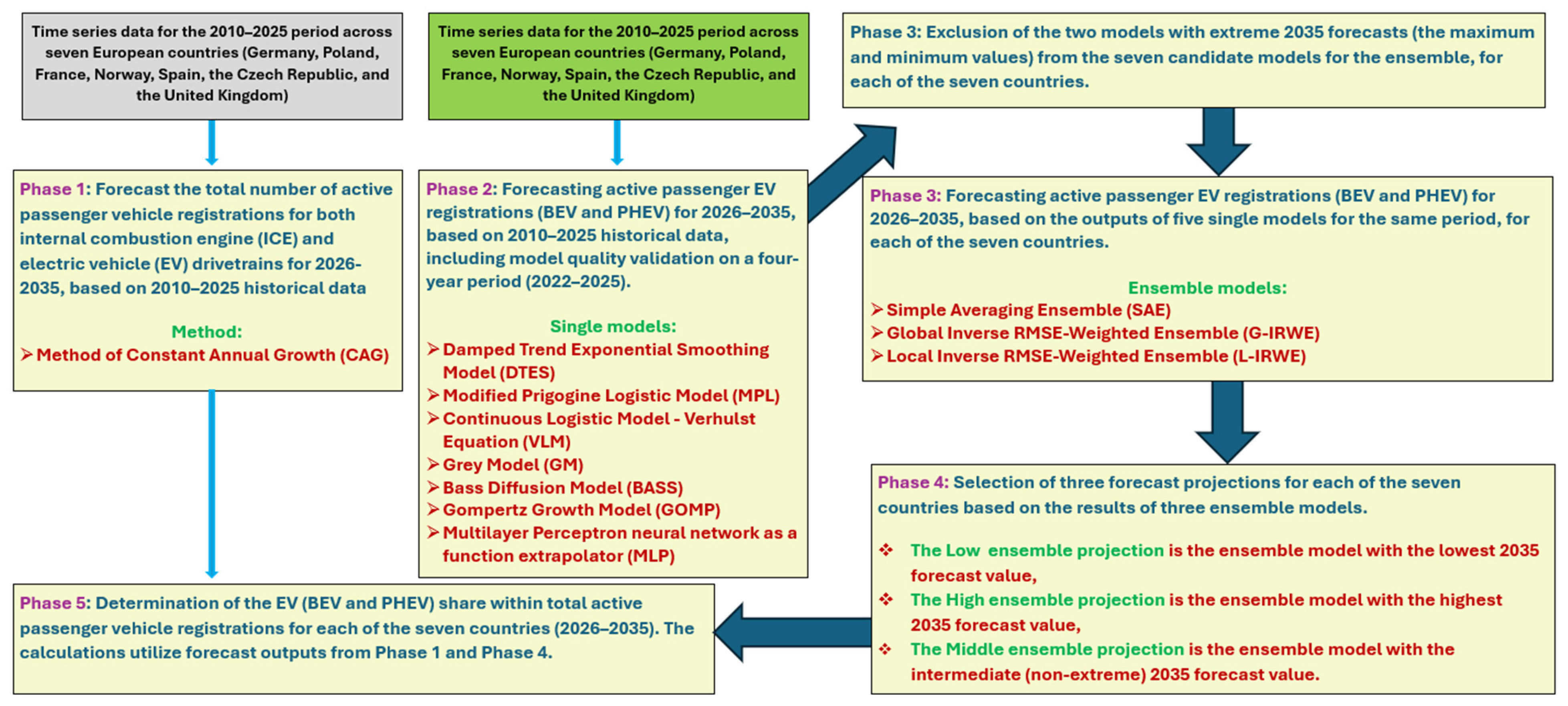
  24. Sbrana, G.; Silvestrini, A. Forecasting with the damped trend model using the structural approach. Int. J. Prod. Econ. 2020, 226, 107654. [Google Scholar] [CrossRef]
  25. Gardner, E.S.; Acar, Y. Fitting the damped trend method of exponential smoothing. J. Oper. Res. Soc. 2019, 70, 926–930. [Google Scholar] [CrossRef]
  26. Piotrowski, P.; Baczyński, D.; Kapler, P. Multi-variant forecasts of the number of electric vehicles in Poland until 2025 and their impact on annual electric energy demand. Przegląd Elektrotech. 2020, 96, 138–141. [Google Scholar] [CrossRef]
  27. Duan, H.; Luo, X. Grey optimization Verhulst model and its application in forecasting coal-related CO2 emissions. Environ. Sci. Pollut. Res. 2020, 27, 43884–43905. [Google Scholar] [CrossRef]
  28. Tong, M.; Duan, H.; He, L. A novel Grey Verhulst model and its application in forecasting CO2 emissions. Environ. Sci. Pollut. Res. 2021, 28, 31370–31379. [Google Scholar] [CrossRef] [PubMed]
  29. Piotrowski, P.; Baczyński, D.; Robak, S.; Kopyt, M.; Piekarz, M.; Polewaczyk, M. Comprehensive forecast of electromobility mid-term development in Poland and its impacts on power system demand. Bull. Pol. Acad. Sci. Tech. Sci. 2020, 68, 697–709. [Google Scholar] [CrossRef]
  30. Liu, S.; Lin, Y. Grey Systems. Theory and Applications; Springer: Berlin/Heidelberg, Germany, 2010. [Google Scholar]
  31. Tattershall, E.; Nenadic, G.; Stevens, R.D. Modelling trend life cycles in scientific research using the Logistic and Gompertz equations. Scientometrics 2021, 126, 9113–9132. [Google Scholar] [CrossRef]
  32. Dudek, G. Multilayer perceptron for short-term load forecasting: From global to local approach. Neural Comput. Appl. 2019, 32, 3695–3707. [Google Scholar] [CrossRef]
  33. Géron, A. Hands-on Machine Learning with Scikit-Learn, Keras, and TensorFlow, 2nd ed.; O’Reilly Media, Inc.: Sevastopol, CA, USA, 2019. [Google Scholar]
  34. Hammam, I.M.; El-Kharbotly, A.K.; Sadek, Y.M. Adaptive demand forecasting framework with weighted ensemble of regression and machine learning models along life cycle variability. Sci. Rep. 2025, 15, 38482. [Google Scholar] [CrossRef]
Figure 1. Time series of the number of active registered electric passenger vehicles (BEVs and PHEVs) from 2010 to 2025 (inclusive) for the seven analysed European countries.
Sustainability 18 05340 g001
Figure 2. Min–max-normalized time series of the number of active registered electric passenger vehicles (BEVs and PHEVs) from 2010 to 2025 (inclusive) for seven analysed European countries.
Sustainability 18 05340 g002
Figure 3. Indexing-normalized time series of the number of active registered electric passenger vehicles (BEVs and PHEVs) from 2010 to 2025 (inclusive) for seven analysed European countries.
Sustainability 18 05340 g003
Figure 4. Log-transformed (logarithmic-scale) time series of the number of active registered electric passenger vehicles (BEVs and PHEVs) from 2010 to 2025 (inclusive) for seven analysed European countries.
Sustainability 18 05340 g004
Figure 5. The workflow of the research stages.
Sustainability 18 05340 g005
Figure 6. Actual values and forecasts of the total number of active passenger vehicle registrations across all drivetrain types, generated by the CAG model for seven European countries.
Sustainability 18 05340 g006
Figure 7. Actual values and the forecasts of the total number of active passenger electric vehicle registrations (BEV and PHEV) generated by the DTES model for the seven European countries.
Sustainability 18 05340 g007
Figure 8. Actual values and the forecasts of the total number of active passenger electric vehicle registrations (BEV and PHEV) generated by the MPL model for the seven European countries.
Sustainability 18 05340 g008
Figure 9. Actual values and the forecasts of the total number of active passenger electric vehicle registrations (BEV and PHEV) generated by the VLM model for the seven European countries.
Sustainability 18 05340 g009
Figure 10. Actual values and the forecasts of the total number of active passenger electric vehicle registrations (BEV and PHEV) generated by the GM model for the seven European countries.
Sustainability 18 05340 g010
Figure 11. Actual values and the forecasts of the total number of active passenger electric vehicle registrations (BEV and PHEV) generated by the BASS model for the seven European countries.
Sustainability 18 05340 g011
Figure 12. Actual values and the forecasts of the total number of active passenger electric vehicle registrations (BEV and PHEV) generated by the GOMP model for the seven European countries.
Sustainability 18 05340 g012
Figure 13. Actual values and the forecasts of the total number of active passenger electric vehicle registrations (BEV and PHEV) generated by the MLP model for the seven European countries.
Sustainability 18 05340 g013
Figure 14. Actual values and the forecasts of the total number of active passenger electric vehicle registrations (BEV and PHEV) generated by the SAE model for the seven European countries.
Sustainability 18 05340 g014
Figure 15. Actual values and the forecasts of the total number of active passenger electric vehicle registrations (BEV and PHEV) generated by the G-IRWE model for the seven European countries.
Sustainability 18 05340 g015
Figure 16. Actual values and the forecasts of the total number of active passenger electric vehicle registrations (BEV and PHEV) generated by the L-IRWE model for the seven European countries.
Sustainability 18 05340 g016
Figure 17. Three projection sets for Germany’s EV share (BEV and PHEV) of total active passenger vehicle registrations (2026–2035), derived from ensemble modeling.
Sustainability 18 05340 g017
Figure 18. Three projection sets for Poland’s EV share (BEV and PHEV) of total active passenger vehicle registrations (2026–2035), derived from ensemble modeling.
Sustainability 18 05340 g018
Figure 19. Three projection sets for France’s EV share (BEV and PHEV) of total active passenger vehicle registrations (2026–2035), derived from ensemble modeling.
Sustainability 18 05340 g019
Figure 20. Three projection sets for Norway’s EV share (BEV and PHEV) of total active passenger vehicle registrations (2026–2035), derived from ensemble modeling.
Sustainability 18 05340 g020
Figure 21. Three projection sets for Spain’s EV share (BEV and PHEV) of total active passenger vehicle registrations (2026–2035), derived from ensemble modeling.
Sustainability 18 05340 g021
Figure 22. Three projection sets for the Czech Republic’s EV share (BEV and PHEV) of total active passenger vehicle registrations (2026–2035), derived from ensemble modeling.
Sustainability 18 05340 g022
Figure 23. Three projection sets for the UK’s EV share (BEV and PHEV) of total active passenger vehicle registrations (2026–2035), derived from ensemble modeling.
Sustainability 18 05340 g023
Table 1. The results in the form of a cross-correlation matrix for the seven analysed countries.
GermanyPolandFranceNorwaySpainCzech RepublicUnited Kingdom
Germany1.000
Poland0.9411.000
France0.9910.9711.000
Norway0.9580.8520.9381.000
Spain0.9790.9850.9970.9121.000
Czech Republic0.9510.9970.9810.8710.9931.000
United Kingdom0.9840.9800.9980.9270.9990.9891.000
Table 2. Comparison of the forecasting methods.
ModelIntuitionKey ParametersOptimizer/EstimationRole in Framework
CAGLinear continuation of average annual changeAverage annual incrementDirect calculationForecasts total passenger vehicle fleet
DTESExponential smoothing with damped trendα, β, φL-BFGS-BSingle EV-stock forecast candidate
MPLNonlinear saturation model based on modified Prigogine/logistic dynamicsR, KL-BFGS-BSingle EV-stock forecast candidate
VLMClassical logistic diffusion with carrying capacityr, KL-BFGS-BSingle EV-stock forecast candidate
GMGrey model for short and incomplete time seriesa, uL-BFGS-B/Nelder–Mead/PowellSingle EV-stock forecast candidate
BASSInnovation–imitation technology diffusionM, p, qL-BFGS-B/TNC/SLSQPSingle EV-stock forecast candidate
GOMPAsymmetric S-shaped diffusionK, a, bL-BFGS-B/TNC/SLSQPSingle EV-stock forecast candidate
MLPConstrained nonlinear function extrapolatorWeights, hidden neurons, activation functionsBFGSSingle EV-stock forecast candidate
SAEEqual-weight trimmed ensembleEqual weightsArithmetic averagingFinal ensemble variant
G-IRWEGlobally RMSE-weighted trimmed ensembleInverse RMSE weightsRMSE over full historical periodFinal ensemble variant
L-IRWELocally RMSE-weighted trimmed ensembleInverse RMSE5 weightsRMSE over last five observationsSensitivity-oriented ensemble variant
CAGLinear continuation of average annual changeAverage annual incrementDirect calculationForecasts total passenger vehicle fleet
Table 3. Forecasted values from seven distinct single models for active passenger EV registrations (BEV and PHEV) in 2035 across seven countries.
Model NameGermanyPolandFranceNorwaySpainCzech RepublicUnited Kingdom
DTES8,063,053------
MPL---3,258,232---
VLM49,534,30927,359,87143,036,5903,212,72226,327,7656,751,48337,551,429
GM24,228,64828,417,40527,819,779-29,148,7457,503,89636,835,316
BASS30,733,27714,534,93227,200,9332,675,09814,655,9713,957,40029,264,791
GOMP16,902,1054,748,80913,780,9782,341,1609,301,0321,655,09615,325,241
MLP-25,959,57010,181,7501,527,4464,652,7954,594,91323,564,561
Table 4. A comprehensive summary of the RMSE values calculated across the entire historical period (2010–2025) for each of the seven countries and the five selected single models.
Model NameGermanyPolandFranceNorwaySpainCzech RepublicUnited Kingdom
DTES123,744------
MPL---184,629---
VLM407,38615,490313,489170,31557,2934545173,316
GM352,3685434157,446-15,473940154,427
BASS216,901542675,78754,74314,09891952,105
GOMP172,135784844,67240,55741,825329523,619
MLP-543731,80331,65013,34096323,100
Table 5. A comprehensive summary of the RMSE5 values, calculated exclusively based on historical data from the final five years of the known period (2021–2025), for each of the seven countries and the five selected single models.
Model NameGermanyPolandFranceNorwaySpainCzech RepublicUnited Kingdom
DTES179,463------
MPL---232,104---
VLM652,46425,134523,810219,98696,6076559276,198
GM194,42510,99291,742-23,10474097,081
BASS279,83211,059124,98978,14420,97777570,808
GOMP229,90812,73876,07967,63260,84129587453
MLP-11,09248,46153,71022,25198911,574
Table 6. The results of ensemble projection selection for each country, derived from the 2035 projections of the three ensemble models.
Forecast ProjectionGermanyPolandFranceNorwaySpainCzech RepublicUnited Kingdom
Low ensemble projectionG-IRWEL-IRWEL-IRWEG-IRWEG-IRWESAEL-IRWE
Middle ensemble projectionL-IRWESAEG-IRWEL-IRWEL-IRWEG-IRWEG-IRWE
High ensemble projectionSAEG-IRWESAESAESAEL-IRWESAE
Table 7. Share of total active passenger vehicle registrations for each of the seven countries (2026–2035) across three forecast horizons—middle ensemble projection.
Forecast HorizonGermanyPolandFranceNorwaySpainCzech RepublicUnited Kingdom
2026 (1 year)8.4%1.8%7.8%37.9%3.6%2.1%9.9%
2030 (5 year)19.2%12.9%17.0%44.2%10.0%10.9%25.0%
2035 (10 year)39.5%68.9%32.3%51.5%27.2%63.4%58.2%
Table 8. Conceptual comparison of the proposed method with related forecasting approaches.
Model CategoryDescription
Single diffusion modelsTransparent and interpretable, but sensitive to model choice and saturation assumptions
Grey modelsSuitable for short and incomplete time series, but may produce unstable long-term extrapolations
Neural-network modelsflexible, but data-demanding and prone to overfitting in very short annual samples
Standard equal-weight ensemblesReduce model-selection risk, but treat all models as equally reliable
Proposed trimmed IRWE frameworkCombines several model families, removes extreme long-term forecasts, and tests alternative weighting schemes; however, it remains trend-based and does not include exogenous explanatory variables
Disclaimer/Publisher’s Note: The statements, opinions and data contained in all publications are solely those of the individual author(s) and contributor(s) and not of MDPI and/or the editor(s). MDPI and/or the editor(s) disclaim responsibility for any injury to people or property resulting from any ideas, methods, instructions or products referred to in the content.