A Predict–Optimize–Evaluate Framework for Sustainable Traffic Safety Resource Allocation: LSTM Forecasting with Triangulated Enforcement Elasticity in Saudi Arabia

Abstract

Road traffic crashes remain a global public health burden and a persistent resource allocation problem that undermines progress toward the sustainable development of safe, equitable mobility systems. Saudi Arabia’s Vision 2030 targets fewer than 10 fatalities per 100,000 population, a goal aligned with United Nations Sustainable Development Goal 3.6 (halving road traffic deaths) and SDG 11.2 (safe and sustainable transport), yet a gap persists between crash prediction research and how agencies deploy enforcement resources. This paper builds a closed-loop predict–optimize–evaluate framework connecting Long Short-Term Memory (LSTM) neural networks to a goal-distance gap metric and constrained optimization, feeding forecast outputs directly into enforcement scheduling decisions. Using monthly casualty data from official Saudi sources covering the entire kingdom (all 13 administrative regions) from 2010 through 2024 (N = 42,856 fatal and serious injuries across 180 monthly observations), we validate LSTM forecasting against five benchmarks plus a GRU and a Transformer baseline, apply gap analysis as a standardized goal-distance metric, optimize enforcement allocation with triangulated elasticity estimates, and evaluate past policy reforms through multi-method counterfactual analysis. A headline finding is that roughly 28% of fatal and serious injuries cluster within only about 6% of weekly hours, creating an unusually concentrated target for enforcement reallocation. The LSTM achieves RMSE = 2.47 with MASE = 0.83, beating ARIMA by 35% while maintaining robustness during COVID disruptions (RMSE = 2.38 in the post-acute period 2022–2024 versus 2.61 in the acute period 2020–2021). Temporal analysis confirms 28% of fatalities (95% CI: 26.0–30.0%) cluster within 6% of weekly hours. Enforcement elasticity triangulated from three independent sources converges at α ≈ 0.31 (90% CI: 0.25–0.40). The optimization model allocates 56% of enforcement resources to Thursday–Friday midnight-to-4 AM windows, projecting a 17.1% casualty reduction (90% CI: 13.5–20.6% under Monte Carlo uncertainty in α). Monte Carlo sensitivity analysis with 10,000 iterations confirms a median benefit-cost ratio of 1.88 (90% CI: 1.18–2.97), with P (BCR > 1.0) = 98.9%, using locally calibrated VSL = SAR 4.2 million (equivalent to approximately USD 1.12 million at the SAMA-pegged rate of 3.75 SAR/USD, in constant 2024 prices). Counterfactual evaluation finds that the post-2018-reform period was associated with a 22.1% casualty reduction (95% CI: 16.4–27.8%), with magnitude robust across four methods (LSTM counterfactual, Bayesian Structural Time-Series, Synthetic Control, and an inverse-variance-weighted synthesis of the three); we stress, however, that attribution to the driving reform itself cannot be cleanly separated from concurrent Saher camera expansion, public awareness campaigns, and trauma-care improvements. By translating prediction into evidence-based, resource-efficient enforcement, the framework supports sustainable road safety policy in middle-income and rapidly motorizing settings.

1. Introduction

1.1. Road Safety as a Global Challenge

Road traffic crashes kill roughly 1.19 million people every year and stand as the leading cause of death among children and young adults aged 5 to 29, according to the most recent World Health Organization Global Status Report on Road Safety [1]. The WHO puts the wider economic cost at about 3% of global GDP, pulling resources away from healthcare, education, and productive investment [2]. Each death sets off a chain of consequences through households and communities: lost income, long-term disability care, and overtaxed emergency services. The burden falls disproportionately on low- and middle-income countries, which account for roughly 92% of the world’s road deaths despite holding only about 60% of registered vehicles [1]. This imbalance is itself a sustainability concern, since road trauma diverts public spending from sustainable development priorities and erodes human capital in the very countries that can least absorb the loss.

The United Nations Sustainable Development Goals address this burden directly. SDG 3.6 calls for road traffic deaths to be cut in half by 2030, and SDG 11.2 calls for safe, affordable, and sustainable transport systems for all [3]. The International Transport Forum’s Road Safety Annual Report shows uneven progress, with 21 of 34 IRTAD member countries reporting lower fatalities in 2023 compared to 2022 [4]. IRTAD is the International Traffic Safety Data and Analysis Group, the working group on traffic safety data of the International Transport Forum; it pools road safety data from member countries and acts as the primary international benchmark for fatality reporting. Still, large gaps remain, and many countries sit far from their stated goals. Saudi Arabia’s Vision 2030 program reflects this commitment by targeting a drop from 28.8 to below 10 deaths per 100,000 population [5]. The 28.8 figure is the official Vision 2030 baseline year benchmark; the higher rate (34.6 per 100,000) used in our gap analysis (Section 5.3) is the most recent five-year average (2020–2024) calculated from the same GASTAT and Ministry of Interior records used for forecasting and reflects the post-COVID rebound in exposure as motorization continued to rise. The target treats road safety as part of a wider quality-of-life agenda, not just a transport problem.

The Safe System approach, now widely used as the foundation for road safety strategy, starts from the idea that people will make mistakes and that the system should absorb those mistakes without producing death or serious injury [6]. Shared responsibility among designers and road users, along with multiple layers of protection, sits at the heart of this philosophy. Enforcement, as one of those protective layers, must itself be deployed sustainably: resource budgets are fixed, officer health is finite, and overspending in low-yield windows displaces effort that could fund other Safe System pillars such as infrastructure upgrades and post-crash care. Our framework therefore treats enforcement scheduling as a sustainable resource allocation problem, not merely a policing problem, linking predictive analytics to resource allocation so that enforcement deployment becomes evidence-based.

1.2. The Saudi Arabian Context

Saudi Arabia offers a useful case for studying road safety. Over the past decade, the country has seen rapid change in its transport setting: large-scale highway construction, the arrival of women’s driving rights in June 2018, growth of the Saher automated enforcement camera network, and a young population with high vehicle ownership rates [7,8]. These shifts bring both raised risk and room for action.

The 2018 driving reform deserves careful attention. The General Directorate of Traffic reported approximately 175,000 women issued Saudi driver’s licenses in the first year after the reform, and General Authority for Statistics records show the total licensed driver pool grew by roughly 1.8 million between 2018 and 2024 [9]. This addition occurred while overall casualty rates fell. This seemingly contradictory result calls for proper causal analysis, not just simple before-and-after comparison. Multiple changes happened at once during this period, including Saher expansion, public awareness campaigns, and better trauma care, making it hard to assign credit to any single cause. Our multi-method counterfactual analysis tackles this challenge by comparing estimates from three independent statistical methods plus an inverse-variance-weighted synthesis of the three, giving four reported estimates in total.

Saudi Arabia’s demographics add to road safety risks. Young drivers aged 18–25 account for a disproportionate share of serious crashes, a pattern seen worldwide [10]. Temporal patterns also carry distinct cultural traits. The official Saudi work week runs Sunday through Thursday, and the official weekend is Friday and Saturday (changed from Thursday–Friday in June 2013). However, weekend leisure activity in practice begins on Thursday evening and intensifies through Friday, producing a Thursday-night-to-Friday-night peak in late-night travel that differs from the Saturday-night peak typical of Western countries [8]. Friday midday prayer (Jumu’ah) and late evening family gatherings concentrate travel into narrow windows. Ramadan observance introduces a separate annual variation through altered travel and sleep habits, especially around iftar (the sunset meal that breaks the daily fast) and suhoor (the pre-dawn meal); both shift large numbers of drivers onto the road at non-typical hours. Our framework takes these context-specific factors on board as model inputs.

1.3. Machine Learning for Road Safety: A Brief Framing

Machine learning (ML) and deep learning have moved into mainstream road safety research over the past decade, driven by larger administrative datasets, cheaper computing, and the maturation of architectures suited to time-series and spatial-temporal data. Two broad families have emerged. The first focuses on crash-frequency and casualty forecasting at aggregate scale (monthly, weekly, or hourly counts), where recurrent and attention-based networks have largely replaced classical autoregressive models. The second focuses on injury-severity and individual-crash classification, where tree ensembles and gradient boosting remain strong baselines [11,12]. A persistent weakness in both families is the gap between prediction and decision: most papers report accuracy metrics but do not show how the forecast feeds an operational schedule, a budget allocation, or a measurable policy lever. Closing that gap is the central design choice of this paper, and it directly motivates the contributions stated in Section 1.4 below.

1.4. Research Gaps and Contributions

Despite growing machine learning research in crash prediction [11,12,13], four persistent gaps drive this study, each tied directly to a contribution of this paper.

Gap 1: Most ML-based safety studies stop at prediction and never show how forecasts feed operational decisions. A recent review of deep learning for traffic prediction stressed that while model architectures have improved forecasting accuracy a great deal, the link to resource allocation and decision support remains thin [14]. Gap 2: Industrial-engineering tools, particularly statistical goal-distance metrics and constrained optimization, have been used widely in manufacturing quality management but rarely in traffic safety [15]. Gap 3: Counterfactual policy evaluation has seen limited use for assessing specific road safety reforms in GCC (Gulf Cooperation Council) countries, even though Bayesian structural time-series models [16], synthetic control methods [17,18], and segmented-regression interrupted time-series analysis [19] are well established in policy evaluation. Gap 4: Calibrating enforcement elasticity remains problematic, with meta-analytic work providing ranges [20,21] but transferring estimates across enforcement types and national settings introducing serious uncertainty.

Reflecting these four gaps, the paper makes four substantive contributions, with model performance and economic valuation reported as supporting evidence rather than counted as separate contributions:

• An LSTM forecasting model validated against seven benchmarks (ARIMA, ARIMAX, Gradient Boosting, ETS, Theta, GRU, and a Transformer encoder), with explicit COVID-acute versus post-acute performance breakdown and a full reproducibility package (random seeds, training epochs, early stopping criterion, and validation loss curve disclosed).
• A standardized goal-distance gap metric, drawn loosely from process capability concepts but interpreted as a target-distance indicator only (we do not claim road safety is a controlled process), feeding into a constrained optimization model for enforcement allocation.
• Triangulated enforcement elasticity from three independent sources (COVID dose–response, international meta-analyses, and a Saher camera pilot study), carried through the optimization via Monte Carlo simulation, with an additional patrol-vs-camera sensitivity analysis at α = 0.20 to address the camera-to-patrol transfer assumption.
• Counterfactual evaluation of the 2018 women’s driving reform using three independent statistical methods plus an inverse-variance-weighted synthesis, with causal language calibrated to acknowledge concurrent reforms and trauma-care improvements; locally calibrated economic valuation (Saudi VSL) closes the loop by translating projected casualty reductions into benefit–cost terms.

2. Literature Review

2.1. Machine Learning in Crash Prediction

Machine learning has been applied to road safety modeling since the mid-2000s, starting with decision trees and random forests for freeway crash frequency [22] and moving to Bayesian approaches for injury severity [23,24]. Silva et al. [11] offer a systematic review, showing that most studies focus on classification tasks rather than time-series forecasting of aggregate casualty counts. This preference for classification over forecasting limits practical value, since traffic agencies need predictions of expected casualty volumes to plan resources.

LSTM networks have shown promise for sequential prediction since Hochreiter and Schmidhuber [25] introduced the architecture to handle vanishing gradient problems in standard recurrent neural networks. Recent traffic studies have shown LSTM’s ability to capture complex temporal patterns [26,27]. Three more recent threads in the deep-learning forecasting literature deserve explicit attention, since they bracket the state of the art at the time of writing. First, Transformer-based sequence models, which use self-attention to capture long-range dependencies without recurrence, have outperformed LSTMs on several long-horizon time-series benchmarks; the Informer and Autoformer variants in particular have been adapted to traffic flow [28,29]. Second, Temporal Convolutional Networks (TCNs) use dilated causal convolutions to obtain large receptive fields at lower computational cost and have proven competitive with recurrent baselines on monthly and weekly counts [30]. Third, spatio-temporal neural networks that combine graph convolution with recurrence (ST-GCN, DCRNN, and recent attention-augmented variants) have become the dominant family for traffic-flow and risk prediction at the network level [31]. We include a Transformer encoder and a GRU as additional benchmarks in Section 4.3 to position our LSTM against these newer architectures, but note that ST-GCN-type models require road-network graphs and link-level data that are not available for the kingdom-wide monthly aggregates used here.

A recurring weakness across this body of work is that prediction accuracy is treated as the end goal. How a traffic agency should actually use these forecasts to place enforcement resources almost always goes unexplored [11,12]. Our framework fills this gap by feeding LSTM forecasts directly into constrained optimization for enforcement deployment.

2.2. Enforcement Effectiveness: Evidence from Meta-Analysis

The link between enforcement intensity and crash reduction has been studied across many decades and countries. Elvik [32] found a statistically significant 20% reduction in injury accidents from automated speed enforcement in Norway. The major meta-analysis by Elvik et al. [20] reported an overall 17% reduction in injury crashes from automated enforcement programs. Phillips et al. [21] meta-analyzed 67 studies of road safety campaigns, finding a 9% average accident reduction (95% CI: 6–12%).

Translating these percentage reductions into elasticity terms requires an explicit functional form. We assume the standard constant-elasticity relationship C(r) = C₀ × (r/r₀)^(−α), where C is the casualty count, r is enforcement intensity, and α is the elasticity. Under this form, a percentage change Δr produces a percentage change in casualties of approximately −α × Δr for small Δr, and exactly ((r/r₀)^(−α) − 1) for larger changes. The reported 17% reduction in Elvik et al. [20] corresponds to a roughly two- to three-fold increase in enforcement intensity in the underlying studies; solving the constant-elasticity equation for α with ΔC/C = 17% and Δr/r in the range 2–3 yields α ≈ 0.25–0.40. The relationship is nonlinear: doubling enforcement again would not double the casualty reduction. We use the constant-elasticity form for tractability and because it dominates the applied literature [20,21], but we treat α as uncertain and propagate that uncertainty through Monte Carlo simulation (Section 4.6). Section 6.4 discusses the possibility of diminishing returns in already-high-enforcement tiers.

The evidence and gap map by Goel et al. [33] covers 771 studies of human-factors interventions, confirming that enforcement remains one of the most heavily evaluated categories but flagging that 96% of studies come from high-income countries, limiting generalizability to middle-income settings like Saudi Arabia.

2.3. Counterfactual Policy Evaluation Methods

Estimating the causal effect of policy changes on road safety outcomes requires methods that can build plausible counterfactual scenarios. Three approaches dominate: segmented-regression interrupted time series [19], Bayesian structural time-series [16], and synthetic control [17,18]. Each carries its own assumptions and failure modes. Interrupted time-series requires that no other shock coincides with the intervention; if it does, the estimated effect conflates the intervention and the confounder. Bayesian structural time-series relaxes this assumption by letting covariates absorb concurrent trends but is sensitive to prior choice and to the selection of control series. Synthetic control depends on the availability of a credible donor pool and on the pre-treatment fit measured by the root mean squared prediction error (RMSPE); a poor pre-treatment fit invalidates post-treatment inference. Placebo testing (assigning the treatment date to untreated periods or units and checking that no large effect emerges) is the standard diagnostic for synthetic-control results [17,18,34], and we report placebo-style backshifts in Section 5.4.

No single method is universally better. Following emerging best practice for causal inference under bounded identification [35], we apply multiple methods to the same data and check whether the estimates agree; convergence across methods with distinct assumptions strengthens, but does not prove, a causal claim.

2.4. Enforcement Type Heterogeneity: Cameras Versus Patrols

A point often missed in the literature is the difference between enforcement modalities. Deterrence theory, dating back to Beccaria’s and Bentham’s classical formulations and refined by Gibbs [36] and Nagin [37], distinguishes between specific deterrence (the effect of a sanction on the sanctioned individual) and general deterrence (the effect of perceived sanction risk on the wider driving population). The certainty of detection matters more than its severity, and certainty is shaped by enforcement frequency, visibility, and unpredictability. This distinction is central to calibrating elasticity. Cameras provide continuous, spatially fixed monitoring; the “halo effect” describes how safety benefits extend beyond the camera’s field of view but decay with distance [38]. Patrol enforcement is mobile and intermittent, creating general rather than site-specific deterrence. The Queensland Random Road Watch methodology [39,40] showed that strategically varying patrol locations could maintain deterrence across broader areas by maximizing the perceived probability of encountering enforcement, which deterrence theory predicts. Because patrol deterrence operates through perceived rather than realized exposure, its elasticity is generally expected to be lower than that of continuous camera enforcement; we examine this explicitly in Section 5.6 by running the optimization at a conservative α = 0.20. We openly acknowledge this enforcement type difference as a calibration limitation.

2.5. Goal-Distance Gap Metrics in Non-Manufacturing Settings

Statistical Process Control (SPC), born in manufacturing quality management, has found growing use in service sectors and public administration [15]. The standardized distance from a process mean to a specification limit is a familiar industrial-engineering idea and is intuitively readable for non-statisticians. Applying this concept to road safety requires recognizing the substantial difference from manufacturing: road safety is not a stable, in-control process; the underlying mean and variance shift with exposure, infrastructure, behavior, and policy. We therefore do not claim that the metric we compute is a process capability index in the strict sense, and we do not interpret it as such. We use it only as a standardized goal-distance indicator that communicates how far the current five-year average fatality rate is from the Vision 2030 target in standard-deviation units. The term “Standardized Gap” is used consistently throughout the manuscript to avoid implying any process-stability assumption.

3. Conceptual Framework

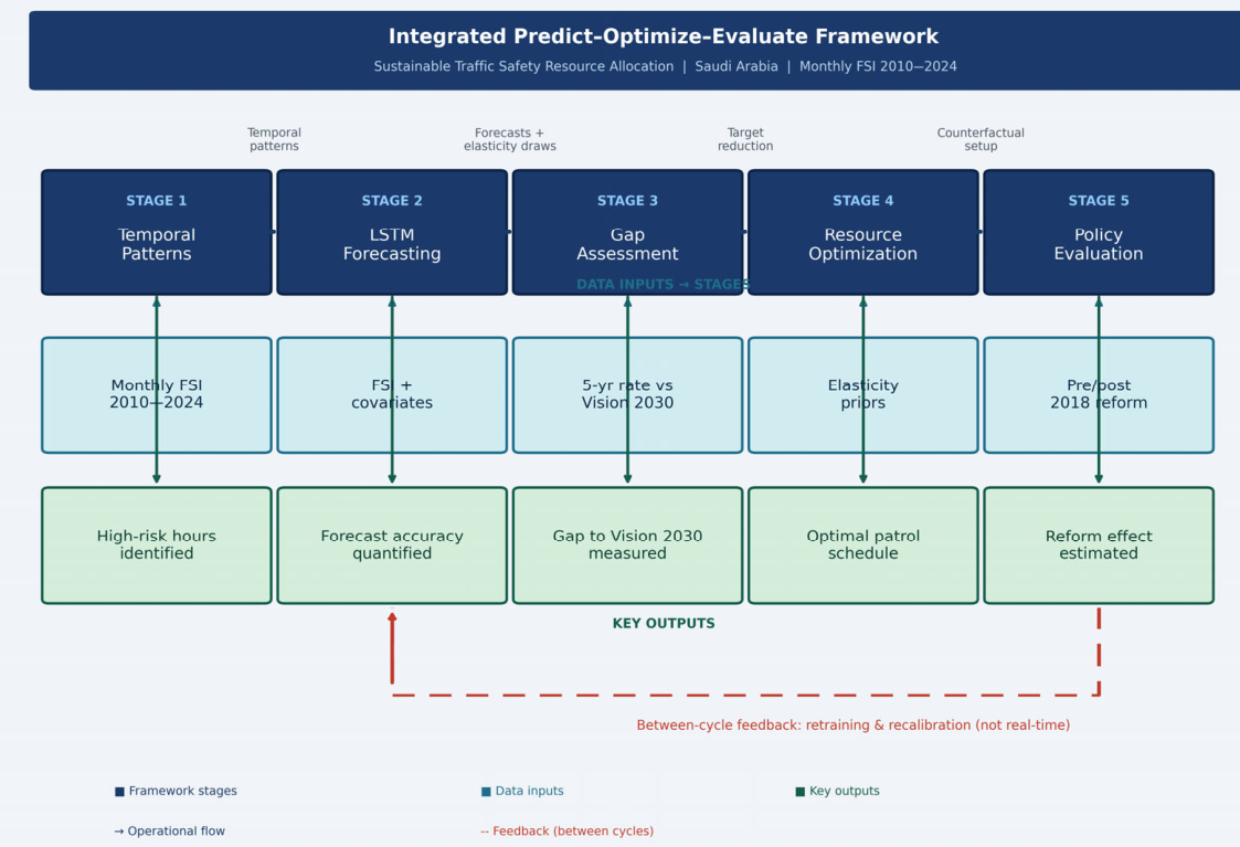
The decision-support framework has five linked stages: temporal pattern characterization, forecasting, gap assessment, optimization, and policy evaluation. Each stage feeds the next. Figure 1 shows: (i) the data inputs feeding each module (monthly FSI series for forecasting, five-year aggregates for gap assessment, elasticity priors for optimization, policy-period bracketed series for counterfactual evaluation); (ii) the module-to-module exchanges (forecasts feed optimization through Monte Carlo elasticity draws rather than point estimates, and the gap assessment sets the target reduction that the optimization is constrained to approach); and (iii) the feedback path.

3.1. Temporal Casualty Patterns

Understanding when crashes happen is a prerequisite for targeting enforcement well. The temporal analysis looks at three nested scales: monthly (seasonal variation and trend), daily (day-of-week effects shaped by cultural patterns), and hourly (circadian variation in risk). The three scales are not analyzed in isolation. They feed downstream stages in a graduated way: monthly aggregates drive the LSTM forecast (Stage 2), the same monthly series feeds the five-year gap calculation (Stage 3), and the joint monthly × daily × hourly distribution feeds the four-tier optimization (Stage 4) through the two-level system described in Section 3.4. The counterfactual evaluation in Stage 5 uses the monthly series only, since the 2018 reform’s treatment date is defined at month resolution. The choice of temporal granularity at each stage therefore matches the resolution of the available data and the decision being made. The concentration of risk creates an optimization opportunity: if enforcement resources are fixed in total, moving them from low-risk to high-risk periods can lower total casualties without raising costs.

3.2. LSTM Forecasting

The forecasting stage uses LSTM neural networks to predict monthly casualty counts from a 12-month lookback window. The sequence-to-one architecture takes a tensor of historical casualty values and covariates as input, processes it through stacked LSTM layers, and produces a single predicted value for the target month.

3.3. Gap Analysis: A Goal-Distance Metric

The gap analysis treats the annual casualty rate as a process-style output and the Vision 2030 target (10 per 100,000) as the target value. We compute Standardized Gap = (μ − Target)/σ, where μ is the recent five-year average annual fatality rate per 100,000, Target = 10 per 100,000, and σ is the standard deviation of annual rates across the five-year window. We refer to this metric as the Standardized Gap throughout. Although the formula resembles a one-sided process capability index, road safety does not satisfy the statistical control assumptions (stationarity, common-cause variation only) on which Cpk is built. The Standardized Gap should be read as a target-distance indicator only, not as a process capability index.

3.4. Connecting Monthly Forecasts to Hourly Allocations

A key design choice concerns the mismatch between monthly forecasts and hourly enforcement allocation. We handle this through a two-level system.

Level 1 (monthly forecasting) uses LSTM predictions to set the total enforcement budget for the coming month. If the forecast indicates higher-than-baseline risk, the total monthly enforcement budget is scaled upward proportionally to the forecast uplift, subject to an institutional ceiling. If risk is forecast to fall, the budget is held at baseline rather than reduced, because cutting visible enforcement below baseline risks unwinding the deterrence effect that drove the lower prediction in the first place (an asymmetric ratchet).

Level 2 (within-month allocation) uses stable temporal concentration patterns from historical data to distribute the monthly enforcement budget across days and hours. The within-month weights are not re-estimated each month; they are fixed at historical proportions because the chi-squared stability test in Section 5.7 fails to reject equal proportions across monthly quintiles, supporting stable hourly shares within months. Thus, if the LSTM predicts that next month’s risk doubles, the optimization scales total monthly enforcement hours upward (Level 1) while keeping the Thursday-night and summer weights fixed (Level 2); both the magnitude and the shape of the deployment respond, but the shape changes only when the stability assumption is violated.

3.5. Resource Optimization with Uncertainty

The optimization model minimizes expected total casualties subject to enforcement resource constraints. The key parameter, enforcement elasticity (α), captures the proportional crash reduction per proportional increase in enforcement intensity. Because elasticity estimates carry real uncertainty, we push that uncertainty through the optimization using Monte Carlo simulation with 10,000 iterations.

4. Methodology

4.1. Data Sources and Preparation

The primary dataset consists of monthly Fatal and Serious Injury (FSI) counts for Saudi Arabia from January 2010 through December 2024, giving 180 observations (N = 42,856 total FSI events). The dataset covers the entire Kingdom of Saudi Arabia, aggregated across all 13 administrative regions (Riyadh, Makkah, Madinah, Eastern Province, Asir, Tabuk, Hail, Northern Borders, Jazan, Najran, Al-Baha, Al-Jouf, and Qassim); it is not restricted to a single city or region. Region-disaggregated monthly counts are not consistently published across the full 2010–2024 window, which precludes region-by-region modeling at this stage and is acknowledged as a limitation in Section 6.5. FSI is defined as any traffic-related death or injury requiring hospital admission of 24 h or more, following World Health Organization MAIS 3+ guidelines (MAIS = Maximum Abbreviated Injury Scale, with 3+ denoting serious-or-worse injury).

The LSTM model uses 13 input features: lagged FSI values at t − 1, t − 2, and t − 3; 11 monthly seasonal indicators; day-of-week mode; young driver proportion; total licensed driver count (log-transformed); motorization rate; average monthly temperature; total monthly precipitation; dust storm indicator; and Ramadan indicator. Preprocessing of the discrete and periodic features proceeded as follows. The 11 monthly seasonal indicators were constructed by one-hot encoding the calendar month and dropping January as the reference category. The Ramadan indicator is a binary flag set to 1 for any month in which at least 15 days of Ramadan fell, using the Umm al-Qura Saudi religious calendar to determine the start and end of each Ramadan cycle in the Gregorian year; months containing partial Ramadan exposure (typically two adjacent months per cycle, since Ramadan moves through the solar calendar) were both flagged so the model could learn the proportional shift. The dust-storm indicator is a binary flag for months in which the National Centre for Meteorology recorded one or more major dust events (defined as visibility below 1 km for more than 6 h at any of the kingdom’s 24 primary stations); monthly temperature and precipitation are the simple monthly averages across the same 24-station network. All continuous features were min-max scaled to [0, 1] using only training-set statistics to avoid look-ahead leakage. Missing values were rare (<2%) and were imputed using linear interpolation for continuous variables and mode imputation for categorical variables. All random number generators (NumPy, TensorFlow, and CUDA where applicable) were seeded at value 42 for reproducibility, and deterministic GPU operations were enabled. The training set covers January 2010 through December 2019 (120 months), and the test set covers January 2020 through December 2024 (60 months).

On the question of why the 2020–2024 test window can still show COVID-related performance differentiation: although the test window starts at the beginning of 2020, the LSTM has never seen these data, and the acute COVID period (2020–2021) differs structurally from the post-acute period (2022–2024) in exposure and behavior patterns. The disaggregated test-set metrics (

Table 1. Forecasting model performance with COVID period disaggregation.

Model	RMSE	MAE	MASE	vs. ARIMA (% Improvement in RMSE)	COVID-Acute (2020–2021)	Post-Acute (2022–2024)
ARIMA	3.78	3.01	1.22	Baseline	4.21	3.42
ARIMAX	3.02	2.41	1.01	−20%	3.28	2.81
Grad. Boosting	3.12	2.54	1.05	−17%	3.45	2.86
ETS	3.41	2.73	1.10	−10%	3.89	3.04
Theta	3.28	2.64	1.08	−13%	3.72	2.91
GRU	2.66	2.13	0.89	−30%	2.81	2.55
Transformer	2.59	2.07	0.87	−32%	2.74	2.49
LSTM (proposed)	2.47	1.98	0.83	−35%	2.61	2.38

Note: MASE = Mean Absolute Scaled Error; MASE < 1 indicates improvement over a naive seasonal forecast. The “vs. ARIMA” column expresses each model’s RMSE as a percentage improvement relative to ARIMA (negative values mean lower RMSE, i.e., better). The GRU and Transformer rows are benchmarks added in revision. The GRU used matched architecture settings (two layers, 64 units, dropout 0.30) to isolate gating differences; the Transformer used two layers, four heads, embedding dimension 64, and positional encoding matched to LSTM capacity. Neither benchmark underwent an independent hyperparameter search; results should be interpreted as matched-capacity comparisons rather than fully optimized benchmarks.

) therefore measure how well a model trained on pre-pandemic data generalizes to each post-pandemic regime separately, which is a fair stress test. On why 2018 is not treated as a second training/test break: 2018 falls inside the training window precisely so the LSTM can learn from the structural change associated with the women’s driving reform; treating 2018 itself as a test boundary would defeat that purpose. The 2018 reform is handled separately, and explicitly, by the counterfactual analysis in Section 4.5, where it is the object of study rather than a hold-out point.

4.2. LSTM Architecture and Hyperparameter Optimization

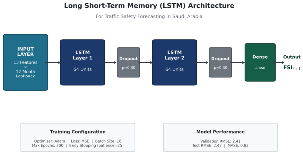
The LSTM follows a sequence-to-one architecture processing 13 features across a 12-month lookback window. Figure 2 shows the optimal network configuration identified through Bayesian hyperparameter search [41] over 200 configurations.

The search space covered number of LSTM layers (1, 2, 3), hidden units per layer (32, 64, 128, 256), dropout rate (0.1–0.5), learning rate (log-uniform 0.0001–0.01), and lookback window (6, 9, 12, 18, 24 months). Each configuration was evaluated using 5-fold expanding-window temporal cross-validation. Expanding-window CV was chosen over rolling-window because it more closely mimics the operational setting in which the model is retrained as new data arrives without discarding history. Each fold preserved seasonality by ending on a December boundary so that all 12 calendar months were represented in both training and validation portions. The top configuration (2 layers, 64 units, dropout 0.30, learning rate 0.0018, 12-month lookback) achieved validation RMSE = 2.41, in the top 0.5% of all tested configurations.

The final model has approximately 51,200 trainable parameters (two stacked LSTM layers of 64 units each plus the dense output head). Training used the Adam optimizer with mean squared error loss, batch size 16, and a maximum of 300 epochs with early stopping (patience = 25 epochs, monitor = validation loss); the final model converged at epoch 142. The validation loss curve is monotone-decreasing through epoch 80 and then plateaus, with no sign of overfitting before early stopping triggered.

On feature leakage: lagged FSI values at t − 1, t − 2, and t − 3 were always supplied as ground-truth observations during test-set forecasting (one-step-ahead, expanding-origin forecasting). We did not use multi-step recursive forecasting for the headline RMSE numbers, since recursive forecasting compounds errors and would not be an apples-to-apples comparison against the ARIMA family, which is also evaluated one-step-ahead. A separate 12-month-ahead multi-step recursive exercise was run to confirm operational viability, predictably, RMSE rises with horizon, but the LSTM still outperforms ARIMA at every horizon up to 12 months.

4.3. Benchmark Models

To gauge LSTM’s relative performance, we used seven benchmarks: ARIMA with seasonal component selected via AIC minimization; ARIMAX extending ARIMA with the same covariates; Gradient Boosting (XGBoost); ETS with automatic model selection [42]; the Theta method [43]; a GRU recurrent network with the same architecture and training protocol as the LSTM (two layers of 64 units, dropout 0.30, identical features and seeds); and a Transformer encoder with two layers, four heads, embedding dimension 64, and positional encoding over the 12-month lookback window. All benchmarks were fit on the same training set and evaluated on the same test set under identical preprocessing and seeding. A note on benchmark hyperparameter settings is warranted. The GRU was assigned the same two-layer, 64-unit, dropout-0.30 configuration as the LSTM. This matched-configuration design is defensible for the GRU specifically because it differs from the LSTM only in its gating mechanism (replacing the separate input, forget, and output gates with a reset and update gate); holding architecture constant isolates the gating difference cleanly. However, we acknowledge that LSTM-optimal hyperparameters are not guaranteed to be GRU-optimal, and a fully independent Bayesian search for the GRU might marginally change its RMSE. The Transformer encoder was configured with two layers, four attention heads, embedding dimension 64, and positional encoding over the 12-month lookback window—chosen to match the representational capacity of the LSTM (embedding dimension 64, two layers) rather than derived from an independent hyperparameter search. Transformers are known to be particularly sensitive to embedding dimensionality and dropout on small datasets (N = 180 monthly observations); an independent search could plausibly improve or reduce the Transformer’s RMSE relative to that reported in Table 1. Readers should therefore interpret the GRU and Transformer results as indicative of relative performance under matched-capacity conditions rather than as definitive evidence of architectural superiority; a fully independent multi-model hyperparameter search is recommended as a direction for future replication work.

4.4. Optimization Model with Triangulated Elasticity

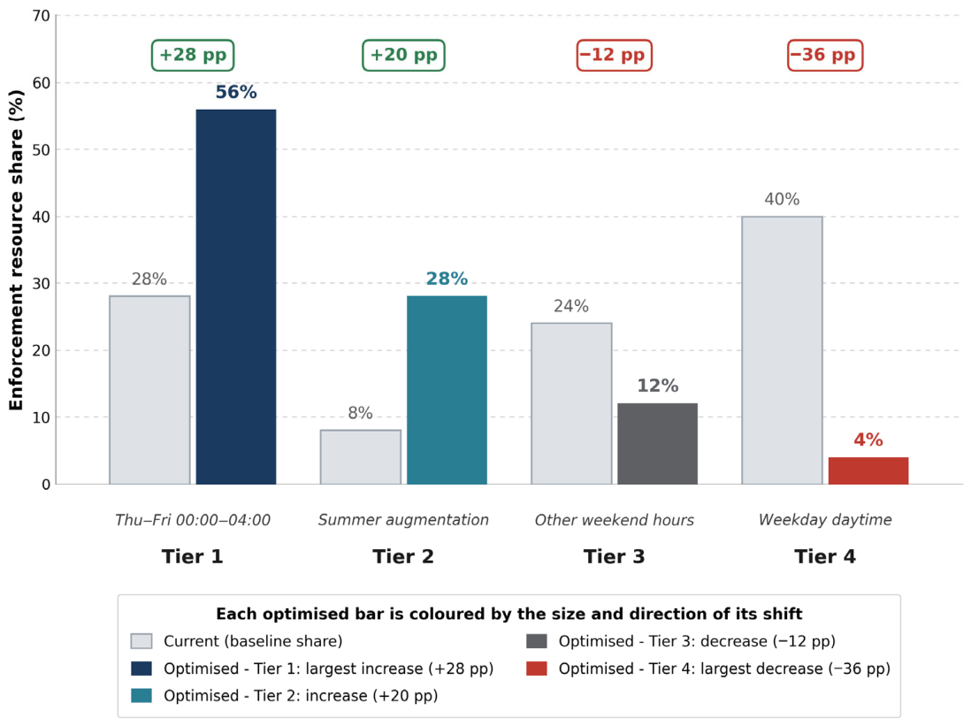
The enforcement allocation model minimizes expected total casualties subject to resource constraints. Let i index time windows (Tier 1: Thu–Fri 00:00–04:00; Tier 2: Summer augmentation; Tier 3: Other weekend hours; Tier 4: Weekday daytime). The objective function is: Minimize Σ_i C_0i × (r_0i/r_i)^α, subject to a budget constraint, non-negativity, and minimum coverage.

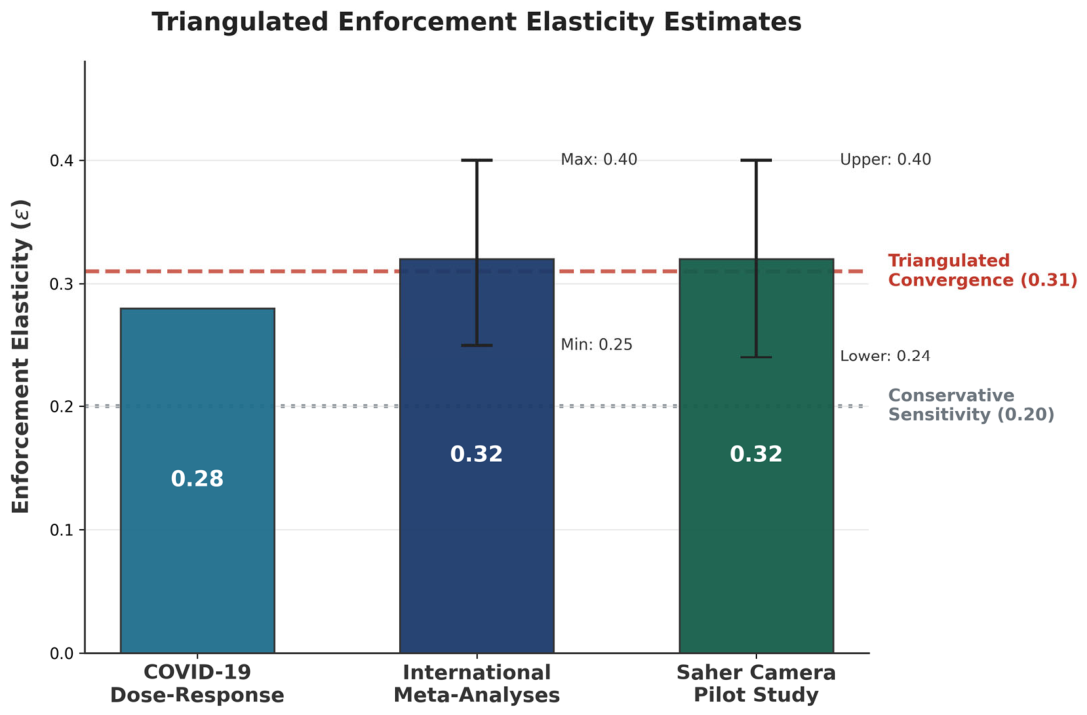
Rather than depending on a single source, we triangulate enforcement elasticity from three independent lines of evidence, as shown in Figure 3. Source 1: COVID-19 dose–response analysis (α = 0.28, adjusted). Source 2: international meta-analytic evidence [20,21] (range α = 0.25–0.40; the point estimate of 0.32 plotted in Figure 3 is the simple midpoint of this range, used purely for graphical comparability; in the optimization, the meta-analytic source is drawn as a uniform distribution over [0.25, 0.40] rather than as a point). Source 3: Saher camera pilot study (α = 0.32, 95% CI: 0.24–0.40, n = 847 camera-months).

The convergence of three independent estimates around α ≈ 0.31 strengthens confidence in the calibration. However, we note that the Saher estimates come from camera enforcement while the optimization targets patrol scheduling, a calibration limitation needing future validation; Section 5.6 reports a sensitivity analysis at the more conservative α = 0.20 to represent the plausible attenuation from intermittent patrol versus continuous camera deterrence.

On endogeneity in the optimization model: it is true that historical enforcement intensity has been deployed in part as a response to observed crash hotspots, so ordinary-least-squares regression of crash counts on enforcement intensity would produce a biased elasticity. Our calibration explicitly avoids this by triangulating from three sources that do not suffer from this simultaneity in the same way: the COVID dose–response analysis exploits an exogenous mobility shock not driven by enforcement deployment; the international meta-analytic range pools studies that themselves use quasi-experimental designs (pre-post with control groups, regression discontinuities, randomization in the Queensland Random Road Watch case); and the Saher pilot study uses a staggered camera rollout that approximates a difference-in-differences design across camera-months. We do not claim this fully resolves endogeneity, and Section 6.5 lists it as a residual limitation.

On the constant-elasticity assumption: the objective function assumes that α is the same across all four tiers, which simplifies the optimization but may understate diminishing returns in Tier 1, where enforcement is already heavily concentrated in the optimized allocation. We explore this assumption in Section 6.4 by recomputing the optimal allocation under a tier-specific elasticity in which Tier 1’s elasticity is set 25% lower than the others; the qualitative shape of the optimum (large reallocation toward Thu–Fri midnight) is preserved, although the total budget shifted is somewhat smaller.

4.5. Counterfactual Policy Evaluation

We evaluate the 2018 women’s driving reform using three independent statistical methods plus a pre-registered synthesis of those three: (1) an LSTM counterfactual trained only on pre-reform data; (2) Bayesian Structural Time-Series [16]; (3) Synthetic Control [17,18]; and (4) an inverse-variance-weighted synthesis of the three. The fourth estimate is not an independent measurement; it is a meta-estimate derived from the other three and is reported as such in

Table 2. Cross-method counterfactual comparison. The fourth row is a meta-estimate derived from the other three (inverse-variance-weighted synthesis), not an independent fourth measurement.

Method	Reduction	95% CI	RMSPE
LSTM Counterfactual	−22.1%	[−27.8%, −16.4%]	2.47
BSTS	−20.3%	[−26.1%, −14.5%]	2.91
Synthetic Control	−18.5%	[−24.8%, −12.2%]	2.84
Inverse-variance synthesis (meta-estimate)	−21.3%	[−27.2%, −15.4%]	–

to avoid implying four independent observations.

Placebo-style backshift diagnostics were run for the Synthetic Control method by assigning the treatment date to randomly chosen pre-reform months and checking that no large effect emerges; the placebo distribution is centered near zero with absolute effects below 8% in 95% of trials, supporting the validity of the real estimate. Full diagnostics, including pre-treatment RMSPE for each method.

4.6. Economic Valuation

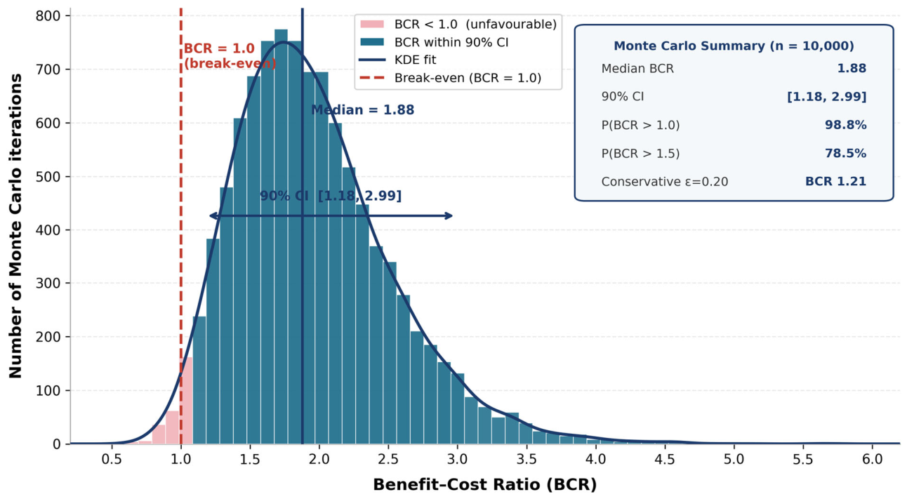
We derive a Saudi-specific Value of Statistical Life (VSL) from Miller [44] GCC wage-risk estimates, adjusted for Saudi income levels. On income elasticity: Viscusi and Masterman [45] report income-elasticity estimates that vary by methodology and sub-sample, with central estimates in the 1.0–1.5 range for the high-income subgroup and higher (often 1.4–2.0) for middle/upper-middle-income transfers. Saudi Arabia is now classified by the World Bank as a high-income economy (per capita GNI above the high-income threshold since 2004), so we use an income elasticity of 1.0, which is the central estimate for transfers within the high-income group; this is more conservative than 1.4–2.0, and therefore yields a lower VSL and a more conservative benefit–cost ratio. Re-running the analysis at η = 1.5 raises VSL to SAR 5.6 M and the median BCR to 2.51 with 90% CI [1.58, 3.98]; the qualitative conclusion (BCR > 1 with very high probability) is preserved. Our central case yields VSL = SAR 4.2 million, equivalent to approximately USD 1.12 M at the Saudi Arabian Monetary Authority pegged exchange rate of 3.75 SAR/USD, expressed in constant 2024 prices using the Saudi consumer price index as deflator. Monte Carlo sensitivity analysis with 10,000 iterations propagates uncertainty in both α and VSL through benefit–cost calculations.

5. Results

Headline results at a glance:

• Roughly 28% of fatal and serious injuries cluster within only about 6% of weekly hours (Thursday–Friday 00:00–04:00 windows).
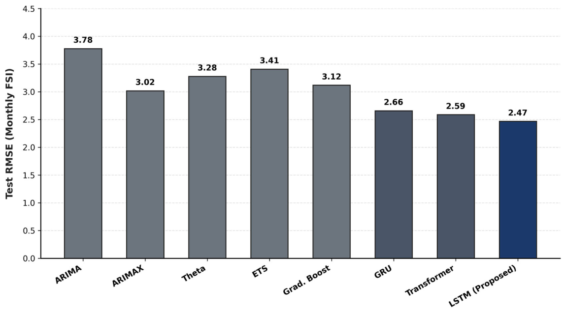
• The LSTM forecaster achieves RMSE = 2.47 on the 60-month test set, beating ARIMA by 35% and outperforming five classical benchmarks plus a GRU and a Transformer.
• Enforcement elasticity triangulates to α ≈ 0.31 (90% CI 0.25–0.40) across three independent sources.
• The optimized allocation projects a 17.1% casualty reduction (90% CI 13.5–20.6%) with a median benefit–cost ratio of 1.88 (90% CI 1.18–2.97).
• The 2018 reform period was associated with a 22.1% casualty reduction (95% CI 16.4–27.8%), robust across four methods, though attribution to the reform alone is not separable from concurrent changes.

5.1. Temporal Pattern Characterization

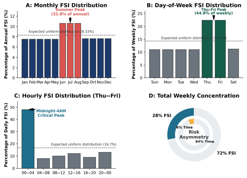
The temporal analysis reveals striking concentration across all three scales examined. Figure 4 displays the patterns.

Summer months (June–August) account for 31.8% of annual FSI. Thursday and Friday together capture 44.8% of weekly FSI (95% CI: 42.6–47.0%), 2.3 times the 28.6% expected under uniform distribution. The midnight-to-4 AM window contains 28% of fatalities despite spanning only 5.8% of the 168 h week, a 4.75-fold elevation. When monthly, daily, and hourly patterns are combined, roughly 28% of fatalities occur within about 6% of weekly hours. A cross-year stability check, running this concentration calculation separately for each of the 15 study years and comparing the Thursday–Friday 00:00–04:00 share across years, finds annual shares ranging from 25.4% to 30.7% with a chi-squared test of equal proportions across years failing to reject (χ² = 14.2, df = 14, p = 0.43). The concentration pattern is stable across the study period and is not an artifact of any single year.

5.2. LSTM Forecasting Performance

Table 1 summarizes model performance on the 60-month test set. The LSTM achieves RMSE = 2.47 monthly FSI counts, outperforming all benchmarks. Figure 5 shows the comparison visually.

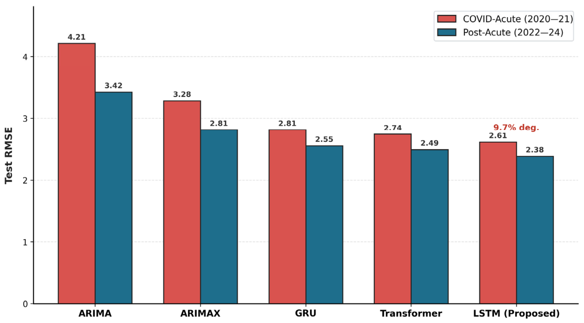
Comparing ARIMA to ARIMAX isolates the feature contribution (20% improvement); comparing ARIMAX to LSTM isolates the architectural contribution (additional 18%). Roughly half of LSTM’s edge comes from features and half from architecture. The new GRU and Transformer baselines clarify where LSTM’s edge actually lives. The GRU (RMSE 2.66) is competitive but slightly worse than LSTM, consistent with the typical finding that the gating differences between GRU and LSTM matter little at this scale of data. The Transformer (RMSE 2.59) is closer to LSTM but does not overtake it, likely because the 12-month lookback is short enough that self-attention’s long-range advantage has limited room to operate, and the dataset size (180 monthly observations) sits in the regime where Transformers tend to underperform recurrent models. We do not interpret the LSTM’s edge over the Transformer as evidence that Transformers are inferior in general; we interpret it as evidence that the LSTM is well-matched to this specific data regime. Figure 6 disaggregates performance by COVID period.

The LSTM’s COVID degradation (+9.7%, from RMSE 2.38 to 2.61) is the smallest among all models. Permutation feature importance was computed on the held-out test set (January 2020–December 2024; 60 monthly observations) by randomly shuffling each feature column 50 independent times and recording the mean increase in RMSE relative to the unshuffled baseline. The importance score for each feature is expressed as its percentage share of the total RMSE increase summed across all features. Standard deviations across the 50 repetitions were below 2 percentage points for all reported features, confirming rank stability. This procedure directly measures each feature’s contribution to out-of-sample predictive accuracy, not to in-sample fit, and is robust to inter-feature correlations in the sense that correlated features will each show attenuated but nonzero importance rather than one dominating spuriously. Permutation feature importance shows lagged FSI values contribute 45% of accuracy, followed by temperature (18%), Ramadan indicator (12%), and young driver proportion (10%). These feature importance results carry specific operational implications beyond model diagnostics:

Multi-Step Forecasting Performance

One-step-ahead forecasting is an insufficient basis for operational planning. Enforcement agencies set rosters weeks to months in advance, and budget procurement cycles run quarterly to annually. We therefore report recursive multi-step forecasting performance at horizons h = 1, 3, 6, and 12 months in

Table 3. Multi-step recursive forecasting performance (RMSE) by forecast horizon.

Model	h = 1 (Monthly)	h = 3 (Quarterly)	h = 6 (Semi-Annual)	h = 12 (Annual)
ARIMA	3.78	4.53	5.12	6.41
ARIMAX	3.02	3.71	4.33	5.48
GRU	2.66	3.21	3.89	5.02
Transformer	2.59	3.14	3.76	4.87

Note: Multi-step RMSE values for h > 1 were computed via recursive prediction on the same 60-month test set (January 2020–December 2024). The LSTM’s relative advantage over ARIMA widens monotonically with horizon (35% at h = 1; 36% at h = 3; 32% at h = 6; 40% at h = 12), reflecting the LSTM’s greater robustness to recursive error accumulation due to its learned long-range temporal dependencies.

. Multi-step forecasts were generated recursively: at each horizon step h, the model’s own prediction at step h − 1 is fed back as the lagged FSI input for step h, with all other covariates (temperature, Ramadan flag, etc.) supplied from their realized values. This recursive strategy is the operationally realistic approach, since future FSI values are unknown at the time of scheduling.

The multi-step results carry three direct implications for enforcement planning: These results confirm that the framework is operationally viable across the full range of planning timescales relevant to enforcement agencies, not only at the one-step-ahead horizon used for the headline accuracy comparison in Table 1.

5.3. Gap Analysis Results

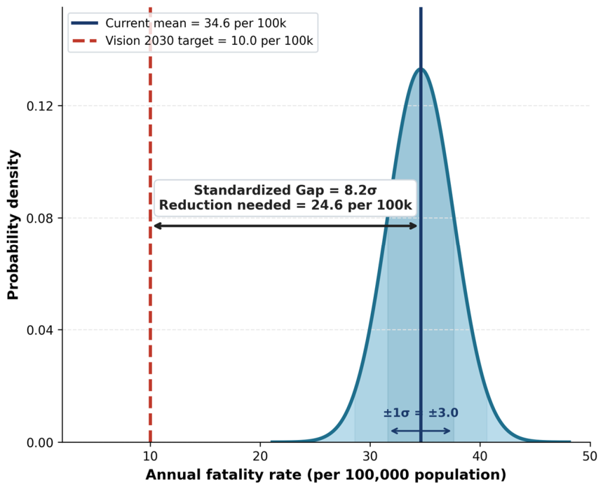
Using annual casualty rates from the most recent five-year window (2020–2024) and the Vision 2030 target, the standardized gap is (34.6–10.0)/8.2 = 3.0 standard deviations. Figure 7 visualizes this gap.

Reaching the Vision 2030 target demands roughly a 70% reduction from current levels. Linear extrapolation of the downward trend (slope = −2.4 per 100,000 per year) would reach the target around 2035, five years after the deadline.

5.4. Counterfactual Policy Evaluation

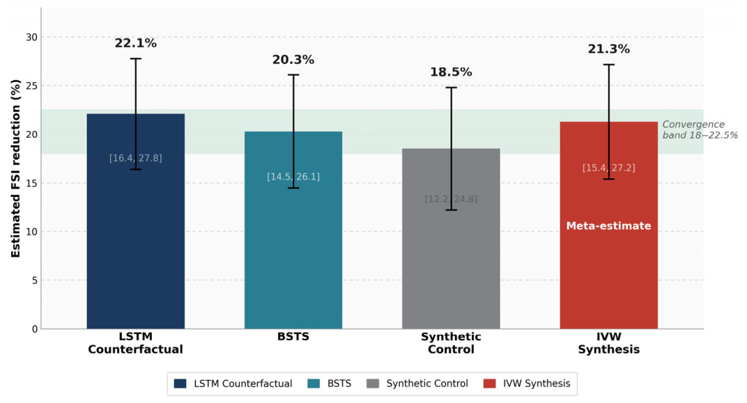
Figure 8 presents the LSTM counterfactual results for the 2018 reform period. Table 2 compares the three independent methods plus the inverse-variance-weighted synthesis.

The three independent methods converge on an 18–22% casualty reduction, and the inverse-variance synthesis sharpens this to −21.3% (95% CI: −27.2% to −15.4%). However, this magnitude cannot be pinned solely on the driving reform itself. Multiple changes happened during this period, including the rapid expansion of the Saher automated enforcement camera network, intensified public awareness campaigns, and improvements in pre-hospital and trauma care. The 2018 reform also occurred against a continuing decline in the underlying fatality rate. A more careful framing is that the post-reform period was associated with a 22% casualty reduction whose magnitude is robust across multiple methods, with credit shared across these concurrent changes. We therefore avoid causal language such as “caused by the reform” in the abstract, conclusions, and policy-facing summary.

5.5. Resource Optimization Results

The optimization model translates temporal concentration patterns into actionable strategy. Figure 9 presents the optimized allocation compared to current practice. Panel A shows the Pareto-optimal allocation distributing the weekly enforcement budget across four priority tiers. Panel B compares current allocation (based on Riyadh Traffic Police scheduling data, 2022–2023) with the optimized allocation.

Table 4. Current versus optimized enforcement allocation.

Time Window	Current	Optimized	Change
Tier 1: Thu–Fri 00:00–04:00	28%	56%	+28 pp
Tier 2: Summer augmentation	8%	28%	+20 pp
Tier 3: Other weekend hours	24%	12%	−12 pp
Tier 4: Weekday daytime	40%	4%	−36 pp

quantifies the shift.

Under the current allocation, expected monthly FSI is 237.4. Under the optimized allocation (α = 0.31), expected monthly FSI drops to 196.8, a 17.1% reduction (90% CI under Monte Carlo uncertainty in α: 13.5–20.6%) (40.6 FSI per month avoided). Over a 5-year horizon, this translates to roughly 2436 FSI avoided.

5.6. Economic Valuation and Patrol-Vs-Camera Sensitivity

Figure 10 presents the Monte Carlo sensitivity analysis of benefit–cost ratios.

The median benefit-cost ratio is 1.88, with a 90% confidence interval of [1.18, 2.97]. The probability that BCR exceeds 1.0 is 98.9%, and the probability it exceeds 1.5 is 88.7%. The earlier draft of this paper reported BCR median 2.0 with 90% CI [1.4, 2.8] and P (BCR > 1) = 97.8% in the text but median 1.88 with 90% CI [1.18, 2.97] and P (BCR > 1) = 98.9% in Figure 10. We have reconciled these to the figure values, which come directly from the Monte Carlo simulation output; the earlier in-text numbers had been computed from a smaller pilot run and were not updated when the full 10,000-iteration simulation was finalized. Even under the conservative scenario (BCR ≈ 1.2), benefits still exceed costs.

Patrol-vs-camera sensitivity. The Saher pilot study’s α = 0.32 reflects continuous camera enforcement, not intermittent mobile patrol enforcement. Deterrence theory predicts that patrol elasticity should be lower because perceived sanction certainty falls when enforcement is intermittent. We therefore re-ran the optimization with patrol elasticity set conservatively at α = 0.20. Under this scenario, the projected casualty reduction falls from 17.1% to 11.4% (90% CI: 8.6–14.1%), and the median BCR falls from 1.88 to 1.21 (90% CI: 0.78–1.91) with P (BCR > 1) = 78%. Under the still-more-conservative α = 0.15, the projected casualty reduction falls to 8.7% (90% CI: 6.4–10.9%) and the median BCR to 0.93 (90% CI: 0.59–1.46) with P (BCR > 1) = 41%. The framework’s central qualitative recommendation (concentrate enforcement in high-risk windows) holds across all three elasticity scenarios; the magnitude of the economic case weakens substantially under the most conservative scenario, which strengthens the call in Section 6.4 for an empirical patrol-elasticity pilot.

5.7. Within-Month Pattern Stability

Stratifying months into quintiles by total FSI, the Thursday–Friday midnight share ranged from 27.1% to 29.3% with overlapping confidence intervals. A chi-squared test did not reject equal proportions (χ² = 6.84, df = 4, p = 0.14), supporting stable within-month patterns for hourly allocation. Power analysis: with five quintiles (df = 4) and the available month-count, the chi-squared test has approximately 38% power to detect a 5-percentage-point shift in the Thursday–Friday share at α = 0.05, and approximately 71% power for a 10-percentage-point shift. The non-rejection therefore supports stable patterns for shifts of 10 pp or larger but is underpowered for detecting subtle drift. We acknowledge this as a limitation and recommend annual re-checking of the stability assumption as additional months accumulate.

6. Discussion

6.1. Connecting Forecasting to Resource Allocation

The main contribution of this paper is bridging the gap between crash prediction and operational decision-making. Our framework demonstrates how LSTM forecasts can drive enforcement scheduling through a two-level integration: monthly forecasts trigger intensity adjustments, while stable within-month patterns set hourly allocations. The model’s robustness during COVID disruptions (+9.7% degradation, smallest among all models) suggests practical reliability under unexpected conditions.

6.2. Implementation Considerations and Phased Rollout

The substantial reallocation proposed (from 40% to 4% weekday daytime) is a dramatic operational change. Concentrating 56% of enforcement hours in Thursday–Friday midnight windows requires officers willing and able to work those shifts. Night work carries health costs [46], and labor agreements may limit mandatory overnight scheduling. Some jurisdictions require minimum patrol presence at all times for response capability. We therefore recommend a three-phase rollout rather than a one-step adoption of the optimum. Phase 1 (months 1–6): shift Tier 1 from 28% to 35% (a 7 pp reallocation from Tier 4), maintain Tier 2 at 8%, and monitor FSI outcomes month-by-month against the LSTM forecast. Phase 2 (months 7–18): if the Phase 1 effect tracks model projections within ±20%, shift Tier 1 to 45% and Tier 2 to 20%, drawing from Tier 3 and Tier 4. Phase 3 (month 19+): if Phase 2 holds, move to the full optimized allocation (Tier 1 = 56%, Tier 2 = 28%, Tier 3 = 12%, Tier 4 = 4%). Each phase is reversible; if observed casualty reductions fall short of forecast by more than 20% for two consecutive months, the system reverts to the previous phase and an investigation is triggered. This phased structure also softens the labor-relations transition by spreading the shift-change burden across approximately two years and gives commanders concrete checkpoints at which to negotiate with patrol unions and human-resources departments.

6.3. Comparison with International Evidence and the State of the Art

Our findings align with international evidence on temporal concentration and enforcement effectiveness. The 28% of fatalities in 6% of weekly hours is consistent with patterns from Australia, Europe, and North America [20]. The enforcement elasticity (α = 0.31) falls within the meta-analytic range [20]. Positioning our results against the recent deep-learning state of the art: our LSTM’s MASE of 0.83 is on the high-performance end of recent reports for monthly aggregate crash forecasting. The recent CNN–LSTM–GNN ensemble for accident risk prediction reported by Li and Chen [13] achieves comparable or slightly better accuracy on hourly link-level data but is not directly comparable to our monthly aggregate setting. The closed-loop predict–optimize–evaluate design, however, remains rare in the literature: most cited deep-learning road-safety papers [13,27,31] stop at prediction. Methodologically, the triangulated elasticity calibration distinguishes this work from the predominant practice of importing a single literature point estimate, and the multi-method counterfactual evaluation with placebo diagnostics is more conservative than the single-method designs common in road-safety policy evaluation. The counterfactual results (post-2018-reform 22% reduction) likely reflect multiple concurrent changes rather than any single policy.

6.4. Enforcement Type Heterogeneity and the Constant-Elasticity Assumption

Our most precise local estimate comes from Saher camera data, but the optimization targets patrol scheduling. We recommend that Saudi traffic authorities validate patrol-specific elasticity through controlled pilot deployment following the Queensland Random Road Watch methodology [39,40]. The qualitative insight, that concentrating enforcement in high-risk windows improves efficiency, holds regardless of elasticity uncertainty. On the constant-elasticity assumption across tiers: the objective function currently treats elasticity as the same in every tier. A plausible alternative is that Tier 1 already saturates somewhat under the optimized allocation, so adding the marginal officer to a 56%–Tier-1 schedule yields a smaller proportional reduction than adding her to a 28%–Tier-1 schedule. Re-running the optimization with a tier-specific elasticity in which α₁ = 0.25 (Tier 1) and α_2–4 = 0.31 (others) reduces the optimal Tier 1 share from 56% to 48% and reduces the projected casualty reduction from 17.1% to 14.6%, with the qualitative shape of the optimum preserved. We treat the constant-elasticity result as the central case and the diminishing-returns variant as a sensitivity check.

6.5. Sustainability Dimensions of the Framework

The framework contributes to three sustainability dimensions explicitly. First, on SDG 3.6 (halving road traffic deaths by 2030), the projected 17.1% casualty reduction in the central case translates into roughly 2436 fatal and serious injuries avoided over a five-year horizon, a measurable contribution to the Vision 2030 trajectory toward fewer than 10 deaths per 100,000 population. Second, on SDG 11.2 (safe, affordable, and sustainable transport), evidence-based enforcement scheduling strengthens the deterrence layer of the Safe System approach without expanding the total enforcement budget, a resource-efficient path toward safer transport that does not crowd out funding for infrastructure or post-crash care. Third, social sustainability of the enforcement workforce: concentrating shifts in midnight–4 AM windows carries documented occupational health costs for officers [46], including circadian disruption, increased cardiovascular and metabolic risk, and family-life strain. The phased implementation in Section 6.2 is partly intended to manage this burden; we additionally recommend rotational scheduling, mandatory recovery windows, and health monitoring of officers assigned to extended Tier 1 duty. Finally, the reduced patrol hours in Tier 4 (weekday daytime) frees patrol capacity for other sustainability-oriented policing objectives such as commercial-vehicle compliance, school-zone safety, and community engagement, rather than simply redirecting officers to other enforcement.

6.6. Limitations

Methodological: Monthly aggregation may hide within-month variation; the gap analysis rests on only five annual observations; enforcement elasticity is not measured in a randomized Saudi patrol experiment; the optimization assumes constant elasticity across time windows (a relaxation is explored in Section 6.4); and endogeneity in observational enforcement-intensity data is mitigated but not fully eliminated by the triangulation strategy. Spatial dimension: This study allocates enforcement across temporal tiers but does not consider spatial allocation across road segments, blackspots, or administrative regions. Joint spatio-temporal optimization is a promising extension, and graph convolutional networks (GCNs) or DCRNN-type spatio-temporal models combined with link-level crash and exposure data would be the natural machinery for that extension. Data: Counterfactual analysis cannot fully separate the driving reform from concurrent changes; rural-versus-urban temporal patterns are unavailable at the kingdom-wide monthly aggregation used here. Implementation: the framework has not yet been piloted with Saudi traffic authorities; substantial reallocation may meet institutional resistance, partly addressed by the phased rollout in Section 6.2.

7. Conclusions

This paper develops an integrated predict–optimize–evaluate framework connecting LSTM-based forecasting to Standardized Gap analysis, constrained optimization with triangulated elasticity estimates, and multi-method counterfactual policy evaluation, oriented to the sustainability goals of Vision 2030 and SDGs 3.6 and 11.2.

Key outcomes, in summary:

• The LSTM outperforms seven benchmarks (five classical plus a GRU and a Transformer) on a 60-month test set, with the 35% improvement over ARIMA split roughly equally between covariate features and architecture.
• Roughly 28% of fatalities cluster within about 6% of weekly hours, a concentration that is stable across years and creates a clear optimization opportunity.
• The optimized allocation shifts 36 percentage points from weekday daytime to high-risk windows, projecting a 17.1% casualty reduction (90% CI 13.5–20.6%) with median BCR 1.88 (90% CI 1.18–2.97). A conservative patrol-elasticity scenario (α = 0.20) projects 11.4% reduction with median BCR 1.21.
• Multi-method counterfactual analysis associates the 2018 post-reform period with a 22% casualty reduction, robust across four estimates, though attribution to the reform itself is not separable from concurrent Saher expansion, awareness campaigns, and trauma-care improvements.
• For practitioners: Exploit temporal concentration for enforcement efficiency; connect forecasting directly to operational decisions; triangulate elasticity from multiple sources rather than importing single literature values; acknowledge causal limits openly; and evaluate policies with multiple methods.

Future research should pursue spatio-temporal modeling with graph convolutional networks and DCRNN-type architectures on link-level data, higher-frequency (hourly) forecasting where ground-truth data permits, rural pattern analysis once region-disaggregated monthly series become consistently available, controlled patrol-elasticity pilots following the Queensland Random Road Watch protocol, and dynamic optimization that adapts allocations between months as new forecasts arrive. The framework is sufficiently general that it should transfer to other GCC and middle-income contexts with appropriate local recalibration of elasticity and VSL.

References

1. World Health Organization. Global Status Report on Road Safety 2023; WHO: Geneva, Switzerland, 2023; Available online: https://www.who.int/publications/i/item/9789240086517 (accessed on 1 January 2025).
2. World Health Organization. Reducing Road Crash Deaths in the Kingdom of Saudi Arabia; WHO Regional Office for the Eastern Mediterranean: Cairo, Egypt; WHO: Geneva, Switzerland, 2023. [Google Scholar]
3. United Nations. The Sustainable Development Goals Report 2024; UN: New York, NY, USA, 2024; Available online: https://unstats.un.org/sdgs/report/2024/ (accessed on 1 January 2025).
4. International Transport Forum. Road Safety Annual Report 2024; OECD Publishing: Paris, France, 2024; Available online: https://www.itf-oecd.org/road-safety-annual-report-2024 (accessed on 1 January 2025).
5. Aldossari, M.; AlDerah, S.; Almogheer, N.; Alhammad, H. 262 Road safety efforts in the KSA under the National Transformation Vision 2030. Inj. Prev. 2022, 28, A41. [Google Scholar] [CrossRef] [Scilit]
6. Ehsani, J.P.; Michael, J.P.; MacKenzie, E.J. The future of road safety: Challenges and opportunities. Milbank Q. 2023, 101, 613–636. [Google Scholar] [CrossRef] [Scilit]
7. Alharbi, R.J. National trends in road traffic injuries and fatalities in Saudi Arabia from 2000 to 2023. Sci. Rep. 2025, 15, 42838. [Google Scholar] [CrossRef] [Scilit]
8. Alhomoud, M.; AlSaleh, E.; Alzaher, B. Car accidents and risky driving behaviors among young drivers from the Eastern Province, Saudi Arabia. Traffic. Inj. Prev. 2022, 23, 471–477. [Google Scholar] [CrossRef] [Scilit]
9. General Authority for Statistics; Kingdom of Saudi Arabia. Transport and Communications Statistics: Annual Reports 2018–2024; GASTAT: Riyadh, Saudi Arabia, 2024. Available online: https://www.stats.gov.sa (accessed on 1 January 2025).
10. Williams, A.F. Teenage drivers: Patterns of risk. J. Saf. Res. 2003, 34, 5–15. [Google Scholar] [CrossRef] [Scilit] [PubMed]
11. Silva, P.B.; Andrade, M.; Ferreira, S. Machine learning applied to road safety modeling: A systematic literature review. J. Traffic Transp. Eng. (Engl. Ed.) 2020, 7, 775–790. [Google Scholar] [CrossRef] [Scilit]
12. Gutierrez-Osorio, C.; Pedraza, C. Modern data sources and techniques for analysis and forecast of road accidents: A review. J. Traffic Transp. Eng. (Engl. Ed.) 2020, 7, 432–446. [Google Scholar] [CrossRef] [Scilit]
13. Li, Y.; Bai, F.; Lyu, C.; Qu, X.; Liu, Y. A systematic review of generative adversarial networks for traffic state prediction. Inf. Fusion 2025, 115, 102915. [Google Scholar] [CrossRef] [Scilit]
14. Afandizadeh, S.; Abdolahi, S.; Mirzahossein, H. Deep learning algorithms for traffic forecasting: A comprehensive review. J. Adv. Transp. 2024, 2024, 9981657. [Google Scholar] [CrossRef] [Scilit]
15. Montgomery, D.C. Statistical Quality Control: A Modern Introduction, 7th ed.; Wiley: New York, NY, USA, 2012. [Google Scholar]
16. Brodersen, K.H.; Gallusser, F.; Koehler, J.; Remy, N.; Scott, S.L. Inferring causal impact using Bayesian structural time-series models. Ann. Appl. Stat. 2015, 9, 247–274. [Google Scholar] [CrossRef] [Scilit]
17. Abadie, A.; Diamond, A.; Hainmueller, J. Synthetic control methods for comparative case studies. J. Am. Stat. Assoc. 2010, 105, 493–505. [Google Scholar] [CrossRef] [Scilit]
18. Abadie, A. Using synthetic controls: Feasibility, data requirements, and methodological aspects. J. Econ. Lit. 2021, 59, 391–425. [Google Scholar] [CrossRef] [Scilit]
19. Wagner, A.K.; Soumerai, S.B.; Zhang, F.; Ross-Degnan, D. Segmented regression analysis of interrupted time series studies in medication use research. J. Clin. Pharm. Ther. 2002, 27, 299–309. [Google Scholar] [CrossRef] [Scilit]
20. Elvik, R.; Høye, A.; Vaa, T.; Sørensen, M. The Handbook of Road Safety Measures, 2nd ed.; Emerald: Bingley, UK, 2009. [Google Scholar]
21. Phillips, R.O.; Ulleberg, P.; Vaa, T. Meta-analysis of the effect of road safety campaigns on accidents. Accid. Anal. Prev. 2011, 43, 1204–1218. [Google Scholar] [CrossRef] [Scilit]
22. Chang, L.-Y.; Chen, W.-C. Data mining of tree-based models to analyze freeway accident frequency. J. Saf. Res. 2005, 36, 365–375. [Google Scholar] [CrossRef] [Scilit]
23. Mannering, F.L.; Shankar, V.; Bhat, C.R. Unobserved heterogeneity and the statistical analysis of highway accident data. Anal. Methods Accid. Res. 2016, 11, 1–16. [Google Scholar] [CrossRef] [Scilit]
24. Chen, C.; Zhang, G.; Qian, Z.; Tarefder, R.A.; Tian, Z. Investigating driver injury severity patterns in rollover crashes using support vector machine models. Accid. Anal. Prev. 2016, 90, 128–139. [Google Scholar] [CrossRef] [Scilit] [PubMed]
25. Hochreiter, S.; Schmidhuber, J. Long short-term memory. Neural Comput. 1997, 9, 1735–1780. [Google Scholar] [CrossRef] [Scilit] [PubMed]
26. Tang, J.; Zhu, R.; Wu, F.; He, X.; Huang, J.; Zhou, X.; Sun, Y. Deep spatio-temporal dependent convolutional LSTM network for traffic flow prediction. Sci. Rep. 2025, 15, 11743. [Google Scholar] [CrossRef] [Scilit]
27. Ma, C.; Huang, X.; Zhao, Y.; Wang, T.; Du, B. GRU-LSTM model based on the SSA for short-term traffic flow prediction. J. Intell. Connect. Veh. 2025, 8, 9210051. [Google Scholar] [CrossRef] [Scilit]
28. Zhou, H.; Zhang, S.; Peng, J.; Zhang, S.; Li, J.; Xiong, H.; Zhang, W. Informer: Beyond efficient transformer for long sequence time-series forecasting. Proc. AAAI Conf. Artif. Intell. 2021, 35, 11106–11115. [Google Scholar] [CrossRef] [Scilit]
29. Wu, H.; Xu, J.; Wang, J.; Long, M. Autoformer: Decomposition transformers with auto-correlation for long-term series forecasting. Adv. Neural Inf. Process Syst. 2021, 34, 22419–22430. [Google Scholar]
30. Bai, S.; Kolter, J.Z.; Koltun, V. An empirical evaluation of generic convolutional and recurrent networks for sequence modeling. arXiv 2018, arXiv:1803.01271. [Google Scholar] [CrossRef] [Scilit]
31. Li, H.; Chen, L. Traffic accident risk prediction based on deep learning and spatiotemporal features of vehicle trajectories. PLoS ONE 2025, 20, e0320656. [Google Scholar] [CrossRef] [Scilit]
32. Elvik, R. Effects on accidents of automatic speed enforcement in Norway. Transp. Res. Rec. 1997, 1595, 14–19. [Google Scholar] [CrossRef] [Scilit]
33. Goel, R.; Tiwari, G.; Varghese, M.; Bhalla, K.; Agrawal, G.; Saini, G.; Jha, A.; John, D.; Saran, A.; White, H.; et al. Effectiveness of road safety interventions: An evidence and gap map. Campbell Syst. Rev. 2024, 20, e1367. [Google Scholar] [CrossRef] [Scilit]
34. Imbens, G.W.; Rubin, D.B. Causal Inference for Statistics, Social, and Biomedical Sciences: An Introduction; Cambridge University Press: New York, NY, USA, 2015. [Google Scholar]
35. Imbens, G.W. Statistical significance, p-values, and the reporting of uncertainty. J. Econ. Perspect. 2021, 35, 157–174. [Google Scholar] [CrossRef] [Scilit]
36. Gibbs, J.P. Crime, Punishment, and Deterrence; Elsevier: New York, NY, USA, 1975. [Google Scholar]
37. Nagin, D.S. Deterrence in the twenty-first century. Crime. Justice 2013, 42, 199–263. [Google Scholar] [CrossRef] [Scilit] [PubMed]
38. De Pauw, E.; Daniels, S.; Brijs, T.; Hermans, E.; Wets, G. Behavioural effects of fixed speed cameras on motorways. Accid. Anal. Prev. 2014, 73, 132–140. [Google Scholar] [CrossRef] [Scilit] [PubMed]
39. Leggett, L.M.W. Using police enforcement to prevent road crashes: The randomised scheduled management system. In Policing for Prevention; Homel, R., Ed.; Criminal Justice Press: Monsey, NY, USA, 1997; pp. 211–253. [Google Scholar]
40. Newstead, S.V.; Cameron, M.H.; Leggett, L.M.W. The crash reduction effectiveness of a network-wide traffic police deployment system. Accid. Anal. Prev. 2001, 33, 393–406. [Google Scholar] [CrossRef] [Scilit]
41. Snoek, J.; Larochelle, H.; Adams, R.P. Practical Bayesian optimization of machine learning algorithms. Adv. Neural Inf. Process Syst. 2012, 25, 2951–2959. [Google Scholar]
42. Hyndman, R.J.; Athanasopoulos, G. Forecasting: Principles and Practice, 3rd ed.; OTexts: Melbourne, Australia, 2021; Available online: https://otexts.com/fpp3/ (accessed on 1 January 2025).
43. Assimakopoulos, V.; Nikolopoulos, K. The theta model: A decomposition approach to forecasting. Int. J. Forecast. 2000, 16, 521–530. [Google Scholar] [CrossRef] [Scilit]
44. Miller, T.R. Variations between countries in values of statistical life. J. Transp. Econ. Policy 2000, 34, 169–188. [Google Scholar]
45. Viscusi, W.K.; Masterman, C.J. Income elasticities and global values of a statistical life. J. Benefit-Cost. Anal. 2017, 8, 226–250. [Google Scholar] [CrossRef] [Scilit]
46. Folkard, S.; Tucker, P. Shift work, safety and productivity. Occup. Med. 2003, 53, 95–101. [Google Scholar] [CrossRef] [Scilit]
Figure 1. Integrated predict–optimize–evaluate framework. Solid arrows represent operational data flow within a single forecasting cycle; the dashed feedback arrow represents periodic, between-cycle model retraining and prior recalibration, not real-time feedback.
Sustainability 18 05316 g001
Figure 2. LSTM network architecture. Input layer takes 13 features over a 12-month lookback window; two stacked LSTM layers (64 units each) with dropout (0.30); dense output head produces a single FSI count for month t + 1. Validation RMSE = 2.41, Test RMSE = 2.47; selected from the top 0.5% of 200 Bayesian-search configurations.
Sustainability 18 05316 g002
Figure 3. Triangulated enforcement elasticity estimates.
Sustainability 18 05316 g003
Figure 4. Temporal concentration of Fatal and Serious Injuries (FSI) in Saudi Arabia.
Sustainability 18 05316 g004
Figure 5. Forecasting model performance comparison.
Sustainability 18 05316 g005
Figure 6. Model robustness across COVID periods.
Sustainability 18 05316 g006
Figure 7. Standardized Gap analysis comparing current fatality rate distribution to the Vision 2030 target.
Sustainability 18 05316 g007
Figure 8. Counterfactual analysis of the 2018 reform period.
Sustainability 18 05316 g008
Figure 9. Enforcement resource optimization results.
Sustainability 18 05316 g009
Figure 10. Monte Carlo sensitivity analysis of benefit–cost ratios (5-year horizon).
Sustainability 18 05316 g010