1. Introduction
In 2024, the UtahForge Engineered Geothermal System (EGS) project completed a 1 km-long horizontal wellbore doublet with L~100 m vertical offset in T~185 °C tight crystalline rock [
1]. The intent was to hydrofracture a series of discrete stress-aligned well-to-well planar pipe-like flow channels through which to pass a working fluid to conductively extract crustal heat as per decades-long conceptual planning [
2,
3,
4,
5]. The overall EGS hydrofracture schema had its field origins in the rift tectonics of Iceland [
2] supplemented by the computational ease of presumed pipe-like fracture-borne fluid flow [
3]. The joint field/computational construct is that of a laminar-flow heat exchanger [
4,
5]. Fundamental to this construct is stress-alignment of laminar-flow structures in an essentially uniformly permeable medium serviced by wellbores passing through the laminar-flow surfaces. EGS stimulation of low-permeability crustal media was thus envisioned as hydrofracture generation of new laminar-flow heat exchange surfaces. The standard EGS scenario is thus pipe-like heat transfer that cannot produce more heat than that contained in the laminar-flow slabs at rates constrained by thermal conduction from crustal slabs to laminar-flow fluid.
A discussion of the UtahForge 2024 EGS stimulation flow data must thus directly recognize that a vast amount of ambient crust field data contradicts the long-envisioned EGS process outlined in [
2,
3,
4,
5]. Since the advent of digital well logs in the 1980s, it has been observed that well-log sequences of crustal rock properties related to crustal fluids have the “pink noise” property that spatial fluctuation power S(k) scales inversely with spatial wave number k over five decades of scale length cm to km:
where wavenumber k ranges over five decades 1/km < k < 1/cm [
6].
Similarly, it is recognized that well-core poro-permeability data from reservoirs worldwide attest the spatial correlation relation between well-core porosity ϕ and the logarithm of well-core permeability κ:
where α is an empirical parameter, and well-core sample intervals are typically 1 foot to 1 m over 10 s to 100 s of meters of formation [
7]. The physical origin of (2) is straightforward combinatorics: for N pores in a unit volume, there are N! = M(N − 1)(N − 2)(N − 3)… ways to connect the pores into a permeability pathway. The Stirling mathematical identity log(N!)~N log(N)–N, (2) simply expresses the poro-permeability combinatorics.
Taken together, (1) and (2) give ambient crust volumetric poro-permeability distribution:
where φ(x,y,z) is a 3D pink-noise porosity array over all relevant scale lengths and α is a field-scale, measurable poro-connectivity formation constant [
8,
9].
It is essential to note that the poro-connectivity parameter α is spatially variable, and as such can logically vary in time with changing crustal conditions. As EGS stimulation is just such a change in crustal condition, EGS can alter α. By (3), increasing α increases permeability without needing to expend energy to increase porosity.
Ambient crust poro-permeability fluctuations (3) occur in geological settings worldwide, directly contradicting the long-standing flow-uniformity assumption made for EGS projects outlined in [
2,
3,
4,
5]. Further, creating laminar-flow planes requires energy to increase the necessary porosity. Accordingly, the view emerges that the 2024 UtahForge EGS flow stimulation data follow flow heterogeneity (3) rather than the until now standard flow-uniformity view.
In the 2024 UtahForge EGS stimulation proceedings, some dozen hydrofracture attempts conducted in both wellbores produced no discernable well-to-well [
1] flow. The UtahForge EGS isolated hydrofracture stimulation format was then abandoned in favor of an open well-to-open well pressurization format. In the final cross-well pressurization setup, all hydrofracture interval packer gear was drilled out of both wells to leave a ℓ~400 m reach of an essentially open wellbore-pair. When the entire ℓ~400 m length of open injection wellbore was pressurized with surface temperature fluid, it was immediately observed that ambient crust temperature T~185 °C fluid flowed from the producer well. The rate of cross-well flow was 30 L/s 3 × 10
−2 m
3/s [
1]. The rate of heat energy produced was:
where ρC is water heat capacity. This steady-state flow was observed for 30 days. With this EGS-stimulation open well-to-open well flow datum, the UtahForge cross-well project achieved the first commercial-grade ambient crust EGS result.
While the UtahForge result effectively eliminates the heretofore standard view of EGS stimulation, three questions arise. First, how did 30 L/s cross-well flow happen when the entire open wellbore was pressurized? Second, how long can the L~100 m offset cross-well flow system sustain the observed Q~20 MWth heat extraction before cooling of the ambient crust heat store diminishes its utility? Third, if the observed 20 MWth heat production quickly cools the cross-well interval, how feasible is it to upscale heat production Q by stimulating flow through the cross-well offsets > L~100 m?
These questions are addressed via a four-step deconstruction of EGS flow stimulation involving fluid–rock interactions in the realistic ambient crust poro-permeability (3). The reality of poro-connectivity parameter α is attested across the value range 2–3 < α
φ < 5–6 for geological formations of mean porosity 0.003 <
φ < 0.2 [
9]. At the same time, crustal poro-perm reality is attested by the intimate relation between (3) and EGS microseismicity, hereafter abbreviated as microearthquakes = Meqs [
10].
Step (i) of the deconstruction of UtahForge EGS flow stimulation data recognizes that wellbore fluid injection is controlled by (3) in a preexisting flow configuration at all scales from centimeters to kilometers. Activating preexisting poro-permeability flow structures can in principle enable flow from anywhere in the injection well to anywhere in the production well. The key feature is that wellbore fluid pipe-like flow ceases at the wellbore radius—nowhere in the crustal medium is fluid flow pipe-like. Further, in step (i) injection flow, Meq stimulation implies pressure-induced irreversible changes in poro-connectivity parameter α that can stimulate flow without creating new porosity.
Deconstruction step (ii) recognizes that fluid flow out of or into a wellbore:
involves collective bulk Darcy flow velocity φv
0 at each point along the open wellbore interval. By conservation of mass, the collective Darcy velocity scales inversely with distance from the wellbore v(r) = r
0v
0//r. Collectively, the Darcy flow fluid is in grain-scale contact with the granular heat store whatever the local complexity of poro-permeability structure.
In deconstruction step (iii), the collective fluid flow increases if local poro-connectivity α parameters increase via local elevated fluid pressurization that extends to larger scale lengths. To first order, increasing poro-connectivity α → α’ > α does not involve increasing porosity and thus to first order does not work against the large confining stresses.
With the recognition of heat advective transport within the stimulation value, EGS deconstruction step (iv) addresses the EGS sustainability question of conductively supplying heat from the surrounding crust. In this step, the UtahForge EGS flow stimulation system is approximated as a single central line-sink of radius R and Q/ℓ radial heat flux boundary condition embedded within a crustal mass of thermal diffusivity D~10−6 m2/s at temperature T. The analytic solution for the thermal mass T(r,t), r > R, serves to estimate the sustainability of UtahForge EGS systems.
Section 2,
Section 3 and
Section 4 elaborate the UtahForge deconstruction.
Section 5 documents the intimate relation of EGS Meqs and crustal poro-permeability (3).
Section 6 illustrates the use of EGS Meq event location data in monitoring the spatially complex EGS flow system. A final section reemphasizes the need to bring crustal physical reality into active EGS play in order to build on the UtahForge 2024 breakthrough. The manifest complexity of crustal flow properties requires developing the EGS system Meq monitoring technology exhibited here.
2. UtahForge EGS Flow Stimulation System
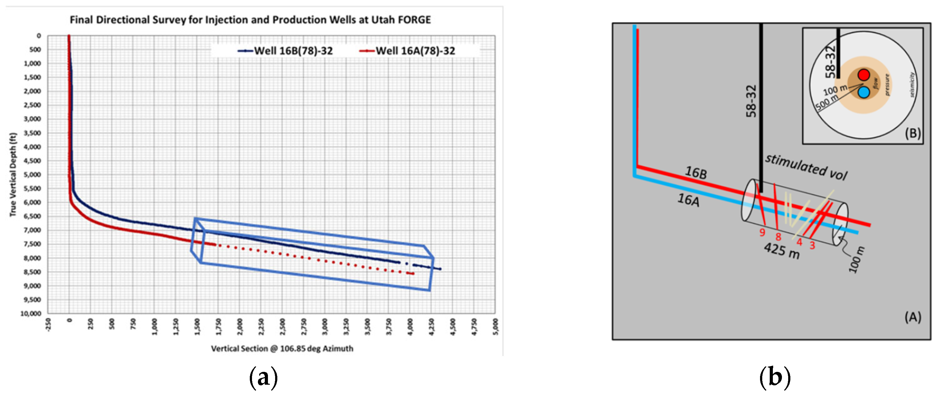
The UtahForge EGS flow stimulation system geometry is sketched in
Figure 1. The UtahForge wells 16B(78)-32, 78-32, and 78B-32 are located within a crystalline basement complex dominated by granitic rocks, specifically Paleozoic-aged granitoids (quartz monzonite/granodiorite). The wells penetrate high-temperature metamorphic and igneous rock, featuring diorite dikes, fracturing, and hydrothermal alteration. Nonetheless, the crustal poro-permeability properties are those given by Equations (1)–(3) [
6,
7,
8,
9,
10].
The sketched crustal volumes are accordingly pervaded throughout by poro-permeability distributions, as given by Equation (3). The blue box in 1a marks the nominal EGS cross-well stimulation understood to be locally stimulated to have poro-connectivity parameter α’ > α, thus enhancing cross-well flow without doing work by increasing porosity.
Figure 1b depicts the well configurations of the stimulation volume.
With reference to
Figure 1, the UtahForge EGS flow stimulation plan was to site a series of isolated hydrofracture sites along the ℓ~400 m horizontal well-pair reach [
1]. As per the long-standing stimulation expectation [
2,
3,
4,
5], well-to-well flow stimulation would occur via discrete stress-aligned planar-like cubic-law flow channels. As recounted in [
1], the events of 2024 showed that after some dozen hydrofracture attempts conducted in both wellbores, no envisioned well-to-well planar flow channels were achieved.
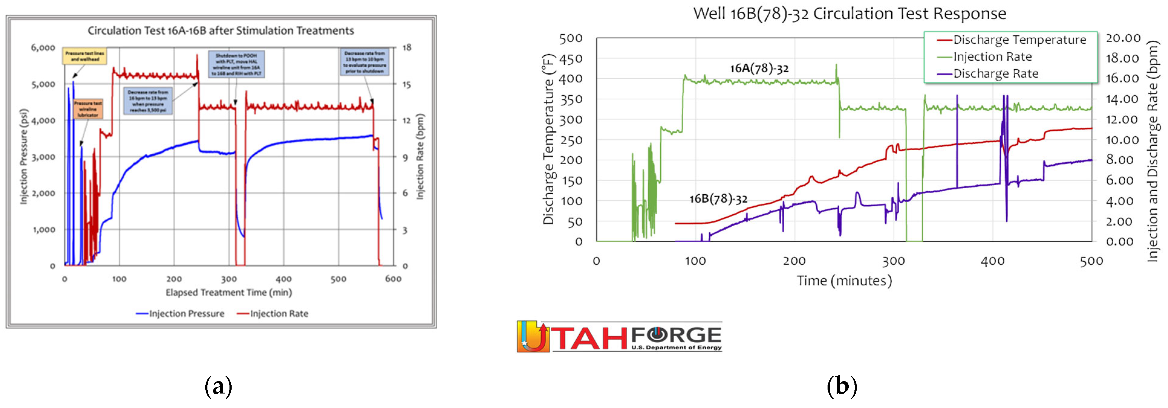
Figure 2 reveals what happened instead. Following a final setup with all hydrofracture interval packer gear drilled out of both wells,
Figure 2a shows that as soon as the injection well pressurization began at 50 min, the open injection wellbore began to flow fluid into the cross-well volume.
Figure 2b shows that with passing time the injector pressure grows and the injector and producer flow rates grow in lockstep.
The producer well flow rate lags the Injector flow rate due to finite fluid flow travel time over the 100 m well-pair separation. Well-to-well flow occurs immediately with pressurization, indicating that the EGS stimulation procedures created well-to-well flow connectivity within the cross-well volume that was accessible to the whole-well pressurization fluid column that was not available to the discrete isolated hydrofrack intervals. It is logical to conclude that well-to-well flow occurs via disseminated volumetric poro-permeability distribution (3) accessed by the 400 m of open hole pressurization fluids.
During the pressurization of the ℓ~400 m length of open injector well shown in
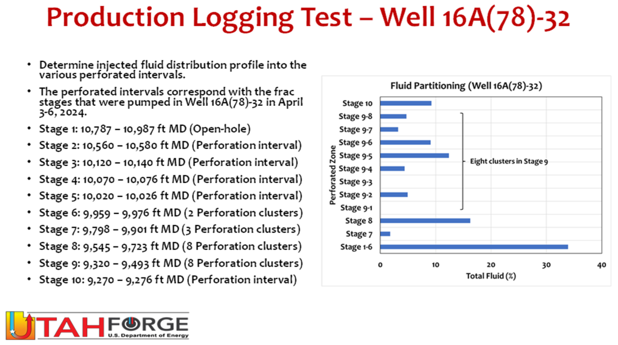
Figure 2, a pressure/flow logging tool was deployed in the injector well to measure the wellbore fluid flow along the length of the pressurization interval.
Figure 3 shows that the wellbore flow (5) along the ℓ~400 m pressurization interval varied as one would expect from variable poro-permeability (3).
The
Figure 3 injector flow irregularity is easily simulated in terms of (3) and (5). The observed open wellbore flows into the ambient crust with a mean and a standard deviation of 11% and 9%, while numerical simulations of distribution (3) return mean values of order 12% with 8% standard deviation.
From (5), it is logical to identify advective flow in the UtahForge EGSG system that yields an effective Peclet number Pe = r
0φv
0/D for thermal diffusive D~10
−6 m
2/s. For r
0φv
0~V/2πℓ~10
−5, the Peclet number for the UtahForge EGS system is Pe~10. For purposes of comparison with the long-standing concept of EGS via conduction processes [
2,
3,
4,
5], the present advection system is 10 times more heat energy-productive than any heat extraction system bound by thermal conduction, which is functionally Pe~1. The UtahForge EGS flow system Pe~10 can be compared with other wellbore-temperature data that are clearly related to crustal flow in fractures. Peclet values 5 < Pe < 10 are observed for isolated wellbore intervals in two wellbore-temperature datasets from naturally occurring deep crustal wellboresp [
12,
13,
14]. It is logical to infer that UtahForge EGS flow stimulation has boosted incidental natural fracture advective flow in the range 5 < Pe < 10 to Pe~10 for the extended decameters-long stimulation interval at the UtahForge site.
The next step considers how the cross-well volumetric domain is stimulated from its initial low-flow condition to the Pe~10 flow condition allowing Q~0 MW heat extraction.
3. Stimulating the Poro-Permeability Crust
The stimulation mechanics by which UtahForge wellbore treatments enhance the cross-well flow documented in
Figure 2 and
Figure 3 are logically due to alterations in the local cross-well poro-permeability field (3). Again, logically, the changes are those involving the least expenditure of deformation energy. It is thus logical that porosity changes are minimal, because increasing porosity necessarily works against the large confining stresses. Far less energy is required to change the poro-connectivity parameter α → α
s > α.
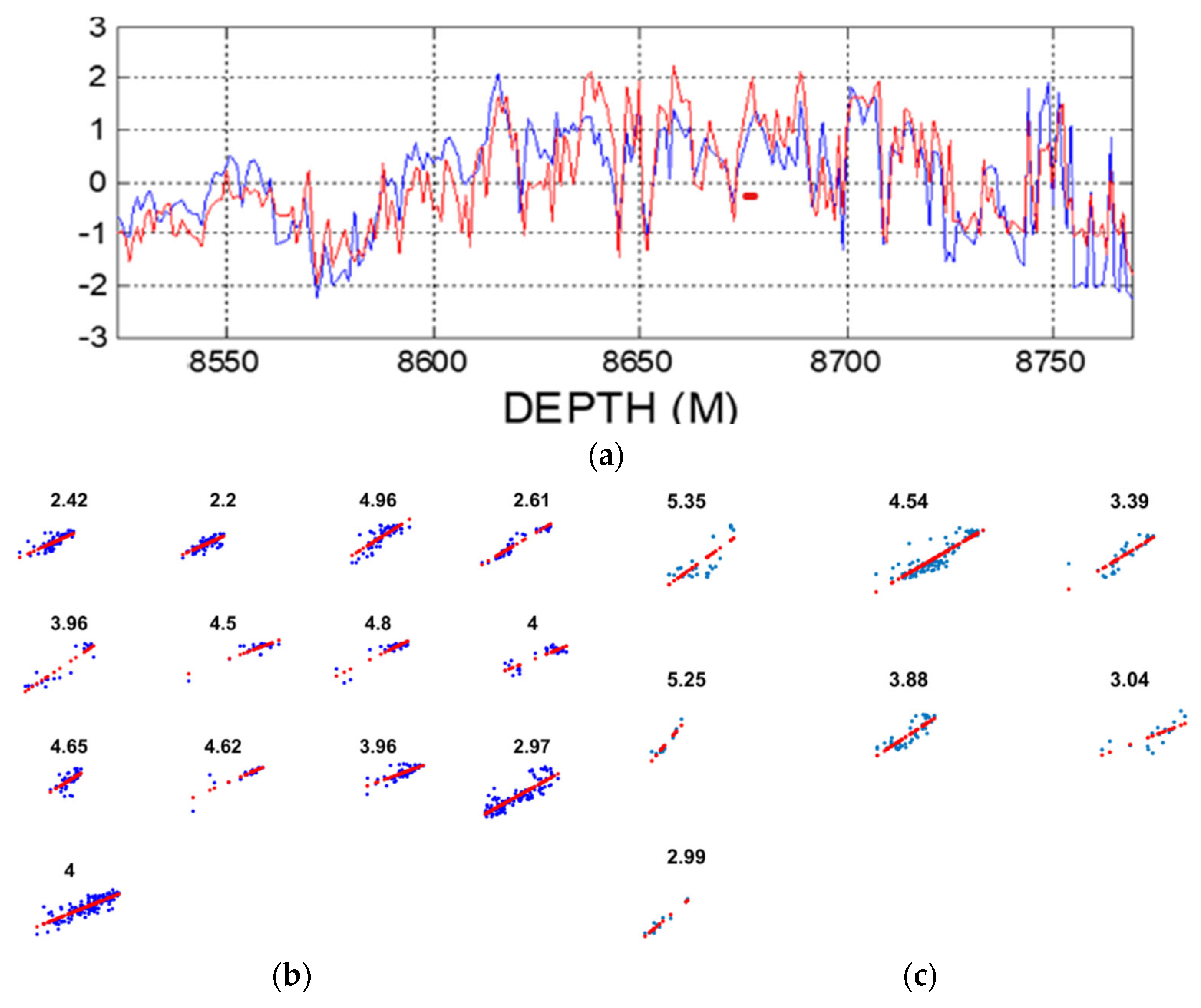
Figure 4 illustrates properties of α at the reservoir scales of meters to hectometers.
Figure 4a plots a sample of 220 well-core porosity and log(permeability) fluctuation data reduced to zero-mean/unit-variance format. The spatial fluctuations of the two traces are 87% correlated. As the expected value for uncorrelated random data is 6%, there is an overwhelming statistical case that Equation (2) has a physical basis, and hence α has physical meaning.
Figure 4b builds on
Figure 4a by numerically evaluating the value of α for a large suite of reservoir well-core data. Each well-core sequence is sorted in ascending porosity value and fit to a linear relation. The slopes of the porosity-ordered version of Equation (2) give a self-consistent suite of α~4 +/−1 values for a large range of reservoir formations.
The point of
Figure 4 data is that Equation (2) represents a semiquantitative measure of a physical crustal property spatial variation that logically extends to temporal variations. While there is no secure way of measuring how and to what extent EGS hydrofrack stimulation attempts to create UtahForge cross-well flow plans, it is both logical and plausible that
Figure 4 spatial variations (Equation (2)) can be materially altered by such pressurization episodes. Such alterations are logically the basis for EGS mechanics.
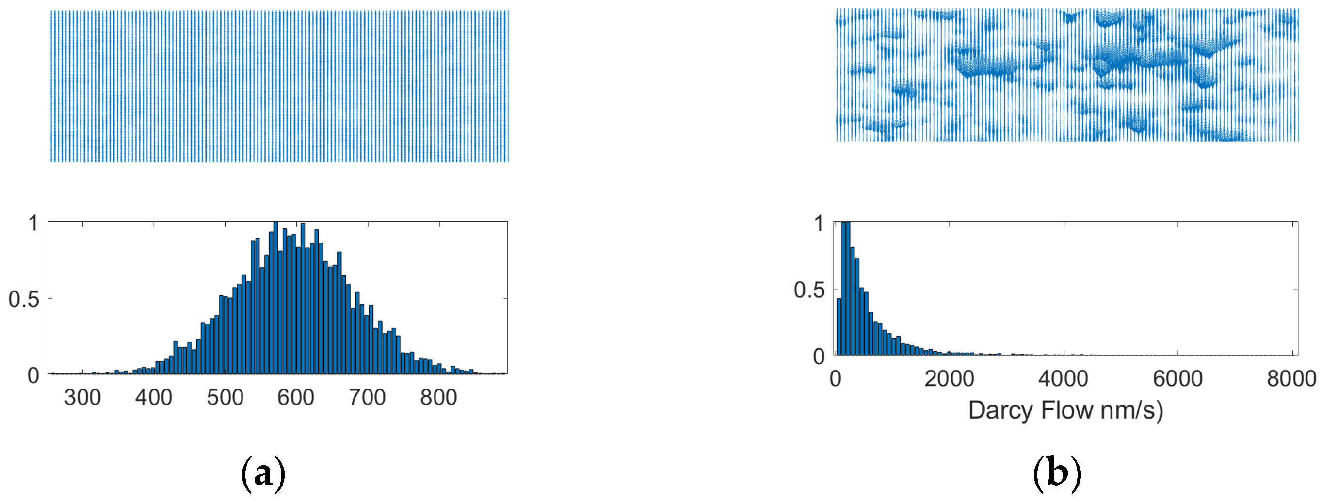
A numerical realization of the poro-connectivity parameter α and its flow stimulation mechanics is illustrated in
Figure 5 [
8]. A cross-well pressure field drives wellbore fluids across a crustal section of poro-permeability (3). Darcy fluid flow velocity for low α (a) shows little spatial variation on the scale of the cross-well gap. The flow velocity distribution is dramatically different for large α (b), where pronounced poro-connectivity structures appear at all scales. Judging from
Figure 4, poro-connectivity parameter α naturally varies in the ambient crust. EGS stimulation concentrates the otherwise natural poro-permeability variations into a local zone of high pore cluster-to-pore cluster flow. It is useful to note that the increased poro-connectivity formally involves no change in porosity. While it is unlikely that no porosity changes occur in physical EGS stimulation processes, the amount of deformation energy expended in increasing α is small compared with systematically creating planar flow-structure gaps, as per the traditional stimulation concept [
2,
3,
4,
5].
An important feature of the
Figure 5 EGS crustal stimulation process is that the concurrent microseismic emissions recorded by local seismic sensors can locate the emission sources in time and space to provide an ongoing image of the stimulation volume. It is seen below how Meq data can provide observational control over the EGS process.
4. Sustaining the EGS Cross-Well Heat Advection
The above deconstruction of the UtahForge EGS stimulation flow system data places heat advection transport comfortably in a natural physical framework characterized by increased poro-connectivity parameter α leading to increased fluid flow velocity and hence increased Peclet number Pe~v(r)r/D~12, r
0 < r < ~50 m. The next step connects the internal wellbore-to-wellbore heat advection flow system sketched in
Figure 1 with its larger external heat volume that conductively feeds heat energy to the internal advection system. Connecting advective heat withdrawal to conductive heat supply defines the EGS system sustainability.
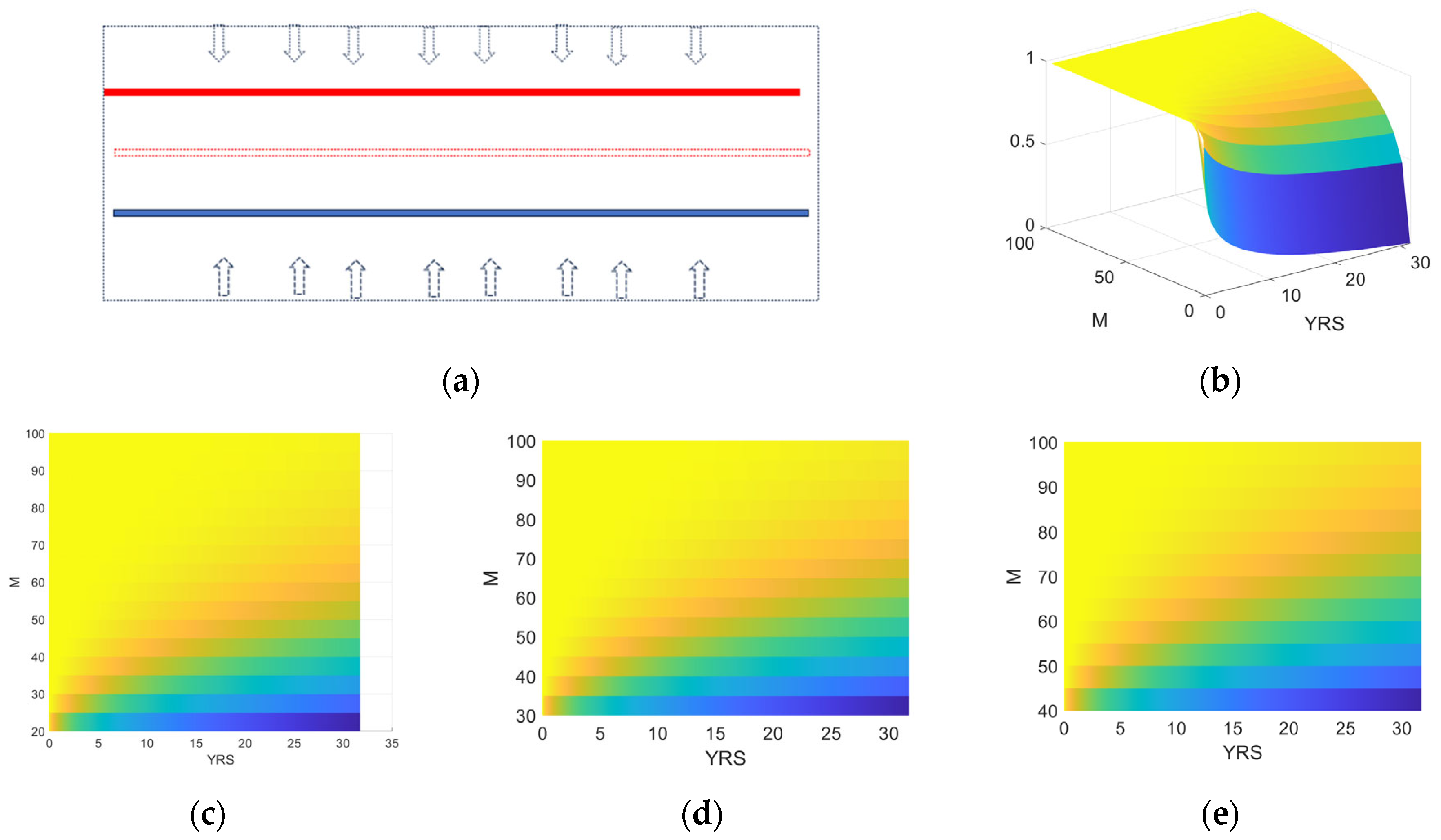
The heat conduction supply is simply approximated by notionally reconfiguring the internal heat transport from well-to-well flow within an R~50 m cylinder that encloses the UtahForge well pair, as sketched in
Figure 6a. For a production well at the notional r~50 m radius, the well retains ambient-temperature fluid. This construct thus estimates the lifetime τ of the UtahForge heat store by solving the heat conduction equation radial heat inflow as a notional central well removes heat at rate:
This notional radial flow and heat flux boundary preserve both the wellbore-based cylindrical heat flow geometry and the internal advection heat transfer of the UtahForge EGS stimulation advection flow system. The wellbore-centric time-evolving crustal temperature field is provided by Carslaw and Jaeger [
15] Equation (7):
where k is spatial frequency,
R is the central wellbore radius, r >
R, and J
0, J
1, Y
0, and Y
1 are Bessel functions of first and second kind and first and second order.
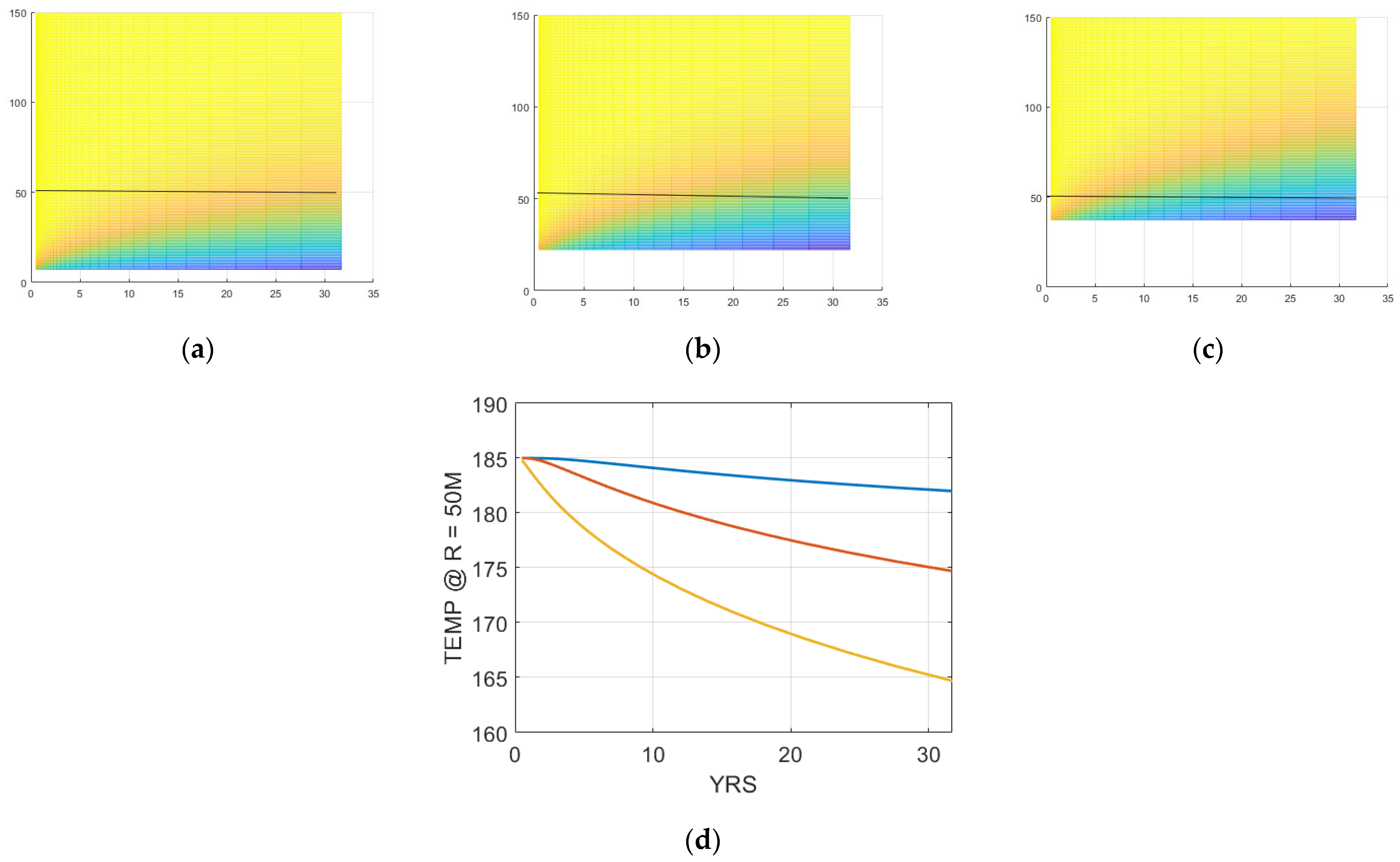
Figure 6b shows the generic/normalized form of Equation (7) temperature T(r,t) for small values of central wellbore radius R in a crustal volume 0 < r < 100 m radius over a period of 30 years. Yellow represents the far-field ambient crustal temperature away from the small central line-sink radius, and blue represents the temperature of the exiting central wellbore fluid as defined by the heat flux boundary condition.
Figure 6c–e are top-down views of temperature distributions for central wellbore radii
R = 20 m, 30 m, and 40 m.
Of immediate interest is the region r~50 m showing the crustal temperature at the radius corresponding to the position of the UtahForge production well. For large radii equivalences for the actual well-to-well heat extraction, heat at r~50 m is seen to decline from ambient temperature due to heat withdrawal outstripping conductive heat renewal. The
Figure 6c–e plots show that the larger the heat withdrawal line-sink radius, the greater the temperature decline at the production position at any given time.
To more quantitatively measure the temperature decline illustrated in
Figure 6 and
Figure 7 numerically simulates the heat withdrawal process for a T = 185 °C ambient crust as seen.
Figure 7a–c numerical simulations fix the near-field heat flux boundary condition Q/ℓ at the internal line-sink radii and the external far-field ambient crust temperature at radius r = 150 m. The top-down temperature fields are shown for three internal line-sink radii, r = 5 m, 15 m, and 25 m. The key interest is shown by (d), where blue, red, and gold traces profile the time-evolving temperature at the r = 50 m radial location of the production well. It is seen that the R = 5 m-radius link-sink has little effect on the production well temperature for up to 30 years of production. By contrast, the R = 25 m-radius line-sink has a significant effect on the production well temperature. For simplicity, the heat flux boundary value is the same for the three internal line-sink radii. Accordingly, the spread of simulated production well temperatures is wider than if the heat flux boundary were adjusted to the same net heat sink extraction rate. In light of the very approximate nature of the computation, allowing the wider production well temperature spread provides a safer illustration of the UtahForge crustal heat store cooling for a Q/ℓ~20 MW/400 m, Pe~10, production well heat energy delivery rate.
Over the spread of
Figure 7 heat extraction scenarios, the simulations indicate first the viability of a decades-long heat delivery for the present UtahForge EGS stimulation system and second raise questions about the feasibility of achieving significantly higher heat production rates Q >> 20 MW, Pe >> 10. Clearly, refining the direct observational knowledge base for the UtahForge system is called for. The next two sections outline the means by which microseismicity data can provide the needed observational capability to physically monitor the EGS flow system evolution.
5. Microseismic Emission Support for EGS Deconstruction
EGS crustal flow stimulation is automatically accompanied by microseismic emissions (Meqs) as the injected high-pressure wellbore fluids are forced into the ambient crust. It has long been supposed that injected high-pressure fluids will hydrofrack the ambient crust along stress-aligned planes of weakness, and that associated microseismic emissions arise from stress-aligned planar slip surfaces resembling fault-zone-like slip mechanics [
16].
Figure 8,
Figure 9,
Figure 10,
Figure 11 and
Figure 12 comprehensively refute this view of EGS microseismicity. Meq slip processes recorded by EGS deep seismic sensors show direct evidence of being embedded in the ambient crust poro-permeability distribution (3). Specifically, UtahForge Meqs such as seen in
Figure 8 and recorded by downhole sensors have the following properties that explicitly refute the long-supposed fault-slip-like properties:
Two-point power-law correlation G(r)~1/r
p, p = 1 (not p = 0) for r = pair-offset (
Figure 9 and
Figure 10).
Bidirectional (not unidirectional) waveform first motions (
Figure 11).
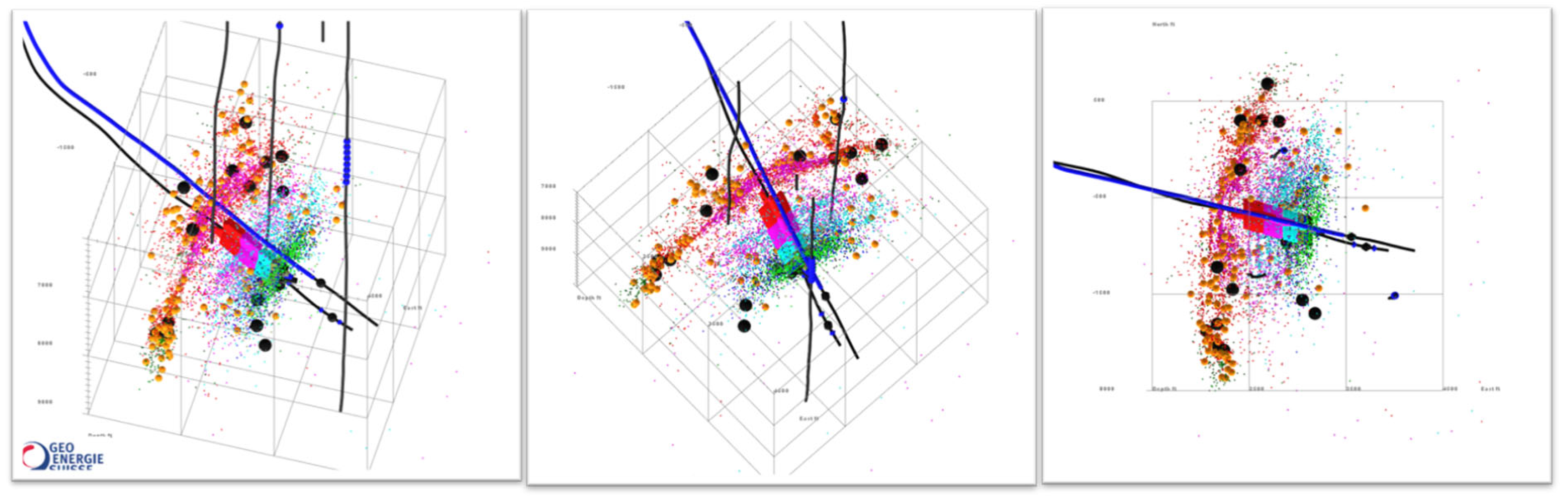
Figure 8 overviews the UtahForge stimulation Meq activity volume sketched in
Figure 1. Each view shows the
Figure 1 well-pair trajectory and the vertical downhole sensor arrays in relation to Meq activity. The cross-well fluid injection excites Meq slip events over a volume that greatly exceeds the target stimulation volumes indicated by rectangular patches superposed on the Meq activity.
Figure 8 gives no evidence that localized hydrofracture interval fluid pressurization is injecting fluid into laminar-flow planes. It is notable that most of the high-magnitude Meqs bear no relation to the EGS target zones. Rather,
Figure 8 shows that stimulation fluids extend into the ambient crust far beyond the cross-well volume sketched in
Figure 1. While stress effects may indeed influence the Meq distribution, they do not explain the lognormal Meq size distribution, the Meq-pairwise distribution, or the bidirectional rather than unidirectional slip mechanics of
Figure 9,
Figure 10 and
Figure 11. These Meq properties accord with the interaction of stimulation fluids with the ambient crust poro-permeability empirics (3).
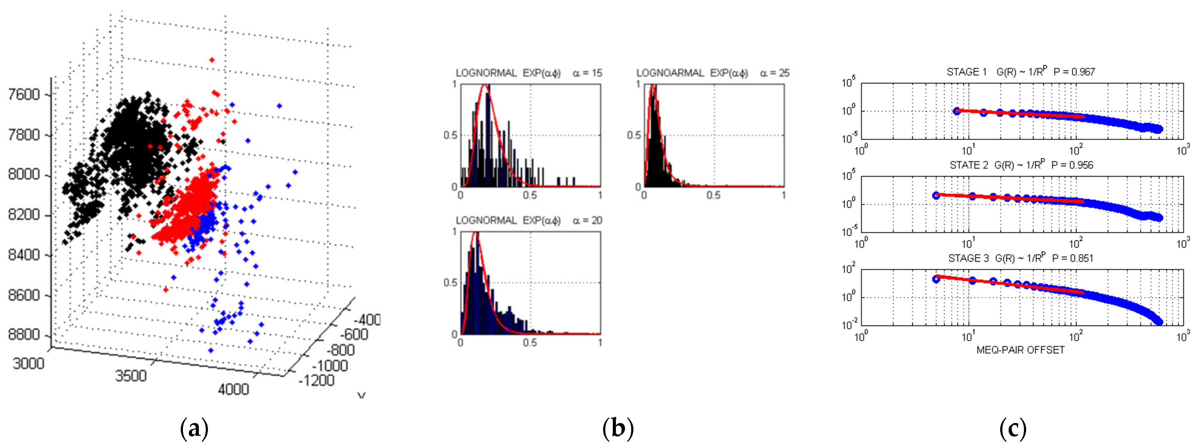
The widely distributed
Figure 9a UtahForge Meq events recorded in 2022 anticipate the widely distributed 2024 Meq data of
Figure 8.
Figure 9b exhibits the lognormal distribution of Meq events, and
Figure 9c exhibits the two-point event-pair spatial correlation distribution function G(r)~1/r, r = Meq event-pair separation. These observed properties refute the standard view of EGS Meqs: (i) Gutenberg–Richter power-law frequency distribution N~10
1-bm,
m = event magnitude, predicts small event numbers increase indefinitely (but are not seen in the data), and (ii) Meq locations have no structure (but instead are seen to have spatial correlation G(r)~1/r).
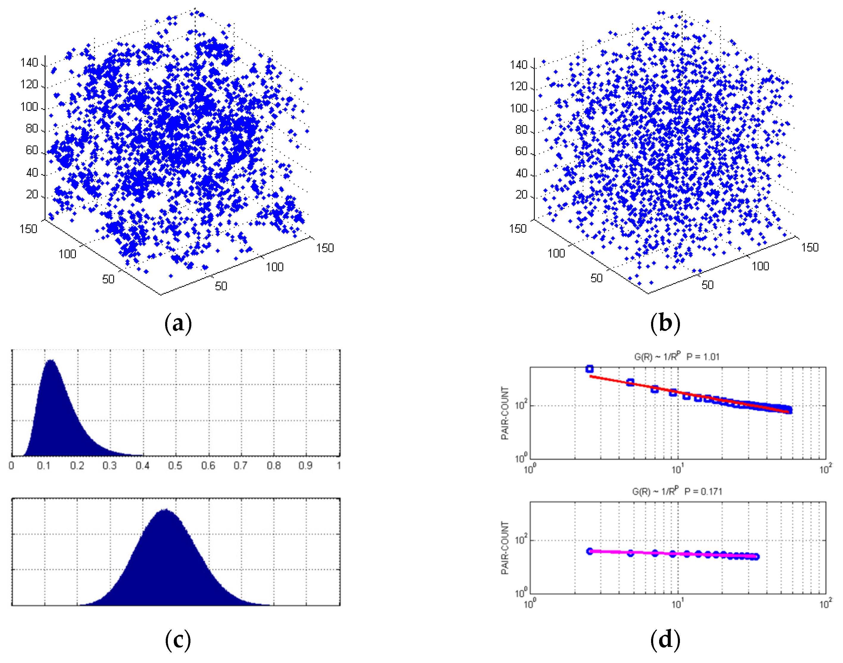
Figure 10 illustrates with synthetic numerics from Equation (3) that the
Figure 9 UtahForge EGS Meq size and spatial correlation property distributions are congruent with the ambient crust poro-permeability size and spatial correlation distributions present in the ambient crust.
Figure 10a Meq events occur as dislocation slip within high-poro-permeability structures in an ambient crust poro-permeability empiric (3).
Figure 10b Meqs are white noise, randomly spaced as regularly assumed in discrete fracture network (DFN) constructions.
Figure 10c shows the lognormal moment distributions of 10a and 10b Meqs. Likewise,
Figure 10d shows the two-point spatial correlation function distribution G(r)~1/r
1 and G(r)~1/r
0 for the 10a and 10b Meqs. The empiric κ(x,y,z)~exp(αφ(x,y,z)) synthetic Meq size and spatial correlation statistics are identical to those of the
Figure 10 UtahForge EGS stimulation Meqs. This statistical congruence validates the working hypotheses that UtahForge EGS stimulations proceed via interacting with the preexisting ambient crust poro-permeability field.
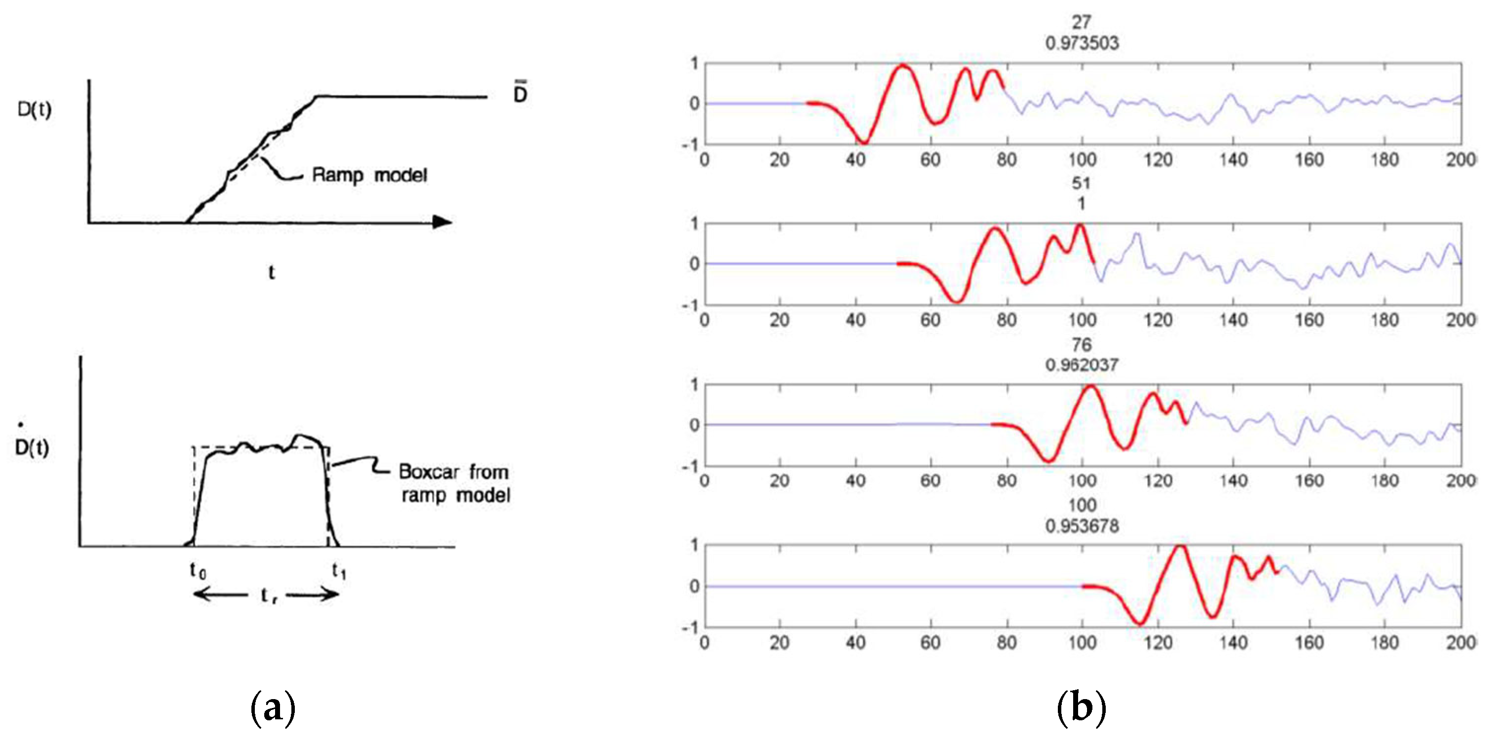
Figure 11 illustrates the seismic first-motion property of EGS Meq events negating standard Meq assumptions [
17]. The standard fault-zone dislocation source slip sketched above has a far-field displacement wave motion denoting slip in one direction only, with slip releasing stress from high to low values along the fault. The observed first displacement motion of EGS Meqs is instead bidirectional, with slip in one direction being followed at a later time by slip in the opposite direction. The observed bidirectional slip is logically due to radial expulsion of high-pressure fluids forced into poro-permeability structures by EGS pressurization followed by radial pressure release. In radial pressure release, fluid-ejection motion pointing to a far-field sensor arrives earlier than the corresponding radial motion away from the sensor.
Tracing the observed UtahForge EGS stimulation Meq emission process to the (3) poro-permeability field establishes the systematic means for surveying the stimulation process. As an application of seismic emission tomography, precise Meq waveform timing of seismic motion recorded by the downhole sensor strings seen in
Figure 8 allows each event to be precisely located in time and space within the stimulation volume. This Meq survey capability can be used in future stimulation exercises to thoroughly explore the flow structure of the present UtahForge stimulation volume and any future stimulation volumes in the ambient crust.
6. EGS Monitoring
Figure 2 and
Figure 3 show that EGS flow data are consistent with an ambient crust that is randomly structured at all scales as per the empirical poro-permeability distribution field (3) attested worldwide by well-log, well-core, and well-flow data across the centimeter-to-kilometer scale range [
6,
7,
8,
9,
10]. The pink-noise structured ambient crust poro-permeability undercuts the assumed easy scalability of EGS in the hypothetical structureless crust. Wellbore injected EGS fluids are seen in
Figure 8,
Figure 9,
Figure 10 and
Figure 11 to interact with the poro-permeability (3) that varies unpredictably at all scales. As such, there is a high probability that any EGS fluid injection path meanders according to the preexisting structured random poro-permeability noise rather than cleaving through a structureless poro-permeability controlled by local stress alignments as assumed in [
4,
5,
16].
In compensation for the scaling pink-noise complexities of the actual ambient crust flow structures, the UtahForge EGS cross-well stimulation flow data connecting Meq seismic emissions to spatially erratic crustal flow allow observers to remotely explore the physical details of EGS mechanics. Referring to
Figure 8, it is apparent that near the EGS stimulation wells there are three vertical wells housing seismic sensor strings. These local seismic sensors record countless Meq seismic emission first-motion wavelets traveling in an essentially uniform seismic wave speed of known logged value. In these circumstances, accurately locating the flow-specific seismic emission source locations is a straightforward exercise in acoustic emission tomography [
18,
19].
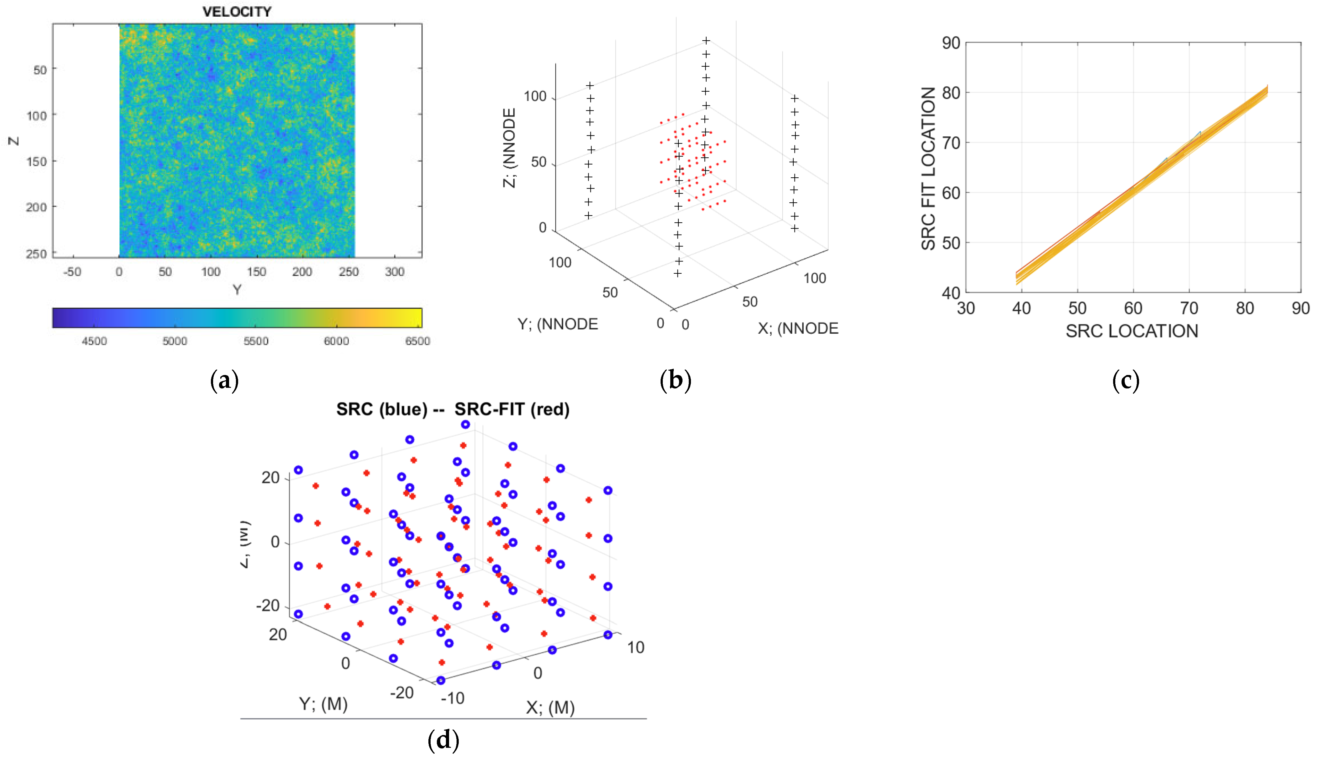
Figure 12 uses synthetic numerics as per
Figure 10 to overview the Meq location inversion process via a numerical simulation of a
Figure 8-scale crustal volume of (3) poro-permeability distribution.
Figure 12a illustrates porosity-driven wave speed fluctuations in a 2D crustal section followed by the
Figure 12b schema of wellbore sensors in the stimulation volume able to record waves emanating from a notional source point asterisk.
Figure 12c shows successive source-sensor travel-time data as circles tracked by travel-time curves fit to data by a least-squares Nelder–Mead fitting algorithm. The Nelder–Mead algorithm returns the spatial location of the source point from the collective sensor travel-time arrival data.
Figure 12d are two views of the fidelity of the inverted source locations (red) in relation to the actual locations (blue) for 30 Meq event locations. These source locations are selected as the 30 largest-value poro-permeability sites in the simulation data cube, and as such conform to the
Figure 10a poro-permeability distribution. The spatial resolution of the inversions is shown respectively at decameter and meter scales. Such Meq data acquisition and processing, as conducted at the UtahForge EGS stimulation site, can routinely confirm in detail the nature and progress of the EGS stimulation process.
On the basis of existing and future UtahForge observation, the
Figure 1 cross-well flow structure sketch can be cast into a generic advection–conduction format in which the radial scale R of the EGS advection–conduction structure can be assessed for a given heat energy flow Q for a given crustal heat reservoir temperature lifetime τ. This result answers the EGS system sustainability problem posed above. The following step determines if the (existing) EGS flow stimulation process can provide a sufficiently large stimulation volume radius R for a given heat production rate Q for a given duration τ.
Figure 7 prospectively calibrates the present UtahForge EGS cross-well flow system at R~50 m as able to produce viable heat for 3–10 years at heat production rate Q~20 MW. Accordingly, systematic Meq observations can validate or adjust the
Figure 7 process. With a firm Meq-based calibration of the present UtahForge EGS cross-well stimulation volume, it is feasible, for instance, to confidently assess what increase of well-to-well offset is needed to increase Q to, say, 40 MW while avoiding badly depleting the heat reservoir over, say, a 20-year period. This capability fully and practically defines EGS system sustainability.
7. EGS Sustainability—Discussion and Conclusions
Deconstruction of the UtahForge EGS flow stimulation data introduces active crustal rock–fluid interactions radically at odds with the passive crustal rock–fluid interaction accepted as normative by the hydrocarbon industry over many decades. It can here be formally recognized that achieving EGS geothermal heat energy extraction requires abandoning the passive engineering flow framework inherited from the hydrocarbon industry.
Historically, hydrocarbon recovery institutionally ignored the spatial complexity of crustal permeability. From the 1930s on, official records of US onshore oil field production showed that well production was effectively Pareto 80–20-distributed [
20]. That is, 20% of wells in an oil field produced 80% of the oil, while 80% of the wells produced 20% of the oil. In 1944, J Law published a comprehensive study of oil field well-core porosity and permeability distributions showing porosity was normally distributed and permeability was lognormally distributed [
12,
21]. In 1945, J Arps noted that oil field well production declines varied over a range of values over time, indicating large spatial variation in reservoir permeability distributions [
22]. In 1956, King Hubbert celebrated the Darcy law centennial by declaring that groundwater flow fluctuations were uncorrelated randomness at all significant scales and hence could be routinely spatially averaged over [
23].
The decades-long prominence of hydrocarbon production has unduly biased concepts of crustal fluid flow relevant to geothermal energy production. Relevant crustal flow misconceptions are deeply rooted in hydrocarbon literature. In spite of the pervasive evidence of large-scale spatial complexities of reservoir flow heterogeneity, e.g., [
24], Warren and Root in 1963 introduced the computation-friendly “sugar cube” model of dual permeability as a substitute for the well-known permeability heterogeneity [
25]. The sugar cube dual-permeability model ignores large-scale flow heterogeneity, yet remains a mainstay of reservoir flow modeling [
26]. In 1972, Bear popularized the computational tactic of representative elementary volume (REV) based on the concept that reservoir complexity was confined to scales smaller than the REV and thus could be ignored by modeling flow in units of REV [
27]. Reservoir flow variations modeling incorporating REVs remains common practice [
28].
Re ignoring the pervasive evidence for large-scale crustal permeability, it is possible to express the hydrocarbon industry flow framework as equivalent to the ambient crust poro-permeability distribution with small values of poro-connectivity parameter α, κ(x,y,z)~exp(αφ(x,y,z)) → 1 + αφ(x,y,z) + (αφ(x,y,z)))
2 + (αφ(x,y,z))
3… This formulation of crustal poro-permeability recovers elements of the well-known Carman–Kozeny relationship popular in the hydrocarbon industry [
29]. However,
Figure 4 provides conclusive evidence that α is not small. Despite its popularity in the hydrocarbon industry, the Carman–Kozeny relationship has little or no field-scale validity.
The general determination of the hydrocarbon industry to ignore poro-permeability heterogeneity in favor of effective passive uniformity is manifested in the industry approach to microseismicity associated with reservoir fluids. While acknowledging that no evidence exists for Meqs to be generated by dislocations along fractures (“One of the curious features of microseismic technology is that no one has ever seen the slippage plane of a microseism that was induced by a hydraulic fracture”), it is widely assumed that Meqs are dislocation slips on fracture surfaces [
30]. A long-standing feature of the hydrocarbon industry approach to crustal fractures is to assume that discrete fracture networks (DFNs) are purely uncorrelated random distributions at all scales [
31]. By definition, uncorrelated randomness can be considered effectively uniform in the sense that any random feature property at a given position will be balanced by its opposite somewhere in the fracture medium. Accordingly, the hydrocarbon industry effectively reverts to the overall assumption expressed by Hubbert [
23] that crustal fluid flow systems are effectively uniform. This working uniformity assumption is exemplified by the treatment of UtahForge EGS stimulation Meq processing of [
16], where all Meqs are assumed to occur on stress-aligned fractures rather than being associated with spatially correlated poro-permeability structures [
17].
Given the evident failure of the hydrocarbon industry to engage accurately with the large-scale crustal poro-permeability complexity and heterogeneity deconstructed from the UtahForge EGS stimulation flow data, it can be concluded that while the hydrocarbon industry crustal fluid flow framework may suffice for hydrocarbon recovery, it is manifestly a poor starting point for thinking about EGS and crustal heat extraction. Let us consider reservoir sustainability in particular. In hydrocarbon recovery, the hydrocarbon reservoir is considered finite, with the hydrocarbons extracted by any profitable method until the reservoir is exhausted and abandoned. There is no thought of hydrocarbon reservoir sustainability: one simply pumps fluids that start out as hydrocarbons and gradually become predominantly water. For geothermal energy recovery, on the other hand, the crustal heat reservoir is effectively infinite, but the first-order question asked of a geothermal project scheme is whether the project is sustainable for long enough to be commercially viable before the heat extracted advectively exceeds the conductive recharge and cools the heat reservoir.
While it is clear that the physical laws of hydrocarbon and geothermal water flow are identical, the practical concepts of crustal reservoir fluid flow are quite different. For energy-rich hydrocarbons, even the most meager of hydrocarbon flows can often pay for a well. For energy-poor steam, only the most vigorous flow can pay for a well.
It follows that a key determinant for both hydrocarbon and steam recovery is reservoir permeability, but in very different ways. For hydrocarbon, provided there is sufficient flow, wells can be drilled uniformly so that each well pays for itself with the bonus that some wells pay far more than low-pay wells. For energy-poor geothermal steam flow, however, most wells are simply “sunk costs,” and failure to find the few high-flow wells dooms the geothermal project. The only way to find the high-flow well sites is to abandon the hydrocarbon recovery drilling mode and fully embrace the physical actuality of ambient crust poro-permeability distribution κ(x,y,z)~exp(αφ(x,y,z)) and use this physical actuality to locate the subsurface flow structures that can provide the requisite steam flow rates over sustainable durations.
In conclusion, the threefold importance of the UtahForge EGS stimulation flow data is first the explicit failure of well-to-well hydrofracks to create well-to-well planar cubic-law flow paths as per the EGS canon; second the success of the 400 m-interval open wellbore pressurization to flow at 30 L/s for 30 days, with well-to-well flow beginning at small initial injector well pressures as seen in
Figure 2; and third the return of deep-sensor Meq waveform data that clearly demonstrate that the Meq slip events do not occur on “fault-like” plane surfaces, but instead are consistent with bidirectional fluid expulsion from over-pressured permeability structures [
17]. Together the UtahForge EGS flow stimulation data collectively provide direct evidence for comprehensive updated perspectives on EGS sustainability. Ambient crust flow heterogeneity exists at all scales from centimeters to kilometers, as expressed by the poro-permeability empiric (3). Equation (3) poses serious problems for upscaling to commercial-grade crustal heat extraction facilities. While the plausible sustainability of the EGS is projected to be denominated in decades, achieving a cross-well separation L > 100 m for such EGS systems becomes increasingly problematic for indefinitely large EGS systems. Fortunately, such matters are open to investigation. The intimate relationship between Meqs generated by EGS fluid interaction with the ambient crust poro-permeability Equation (3) distribution provides powerful observational means by which to reliably validate, survey, and monitor the sustainability of present and future EGS stimulation projects.