A Multi-Objective MATLAB–FEM Framework for Sustainable Impressed-Current Cathodic Protection of DC-Electrified Railway Infrastructure

Abstract

Stray-current corrosion from DC-electrified railways drives premature failure of buried metallic infrastructure (pipelines, foundations, tunnel reinforcement), causing resource waste, repair-driven carbon emissions and service disruptions that undermine the sustainability of urban transit corridors. Conventional impressed-current cathodic protection (ICCP) design relies on uniform-anode rules of thumb or closed commercial codes that cannot quantify the trade-off between protection uniformity, energy use and hardware cost. We present an open MATLAB framework that couples a custom 3D finite element method (FEM) solver with multi-objective particle swarm optimisation (MOPSO) and minimises three competing objectives simultaneously: total impressed current, RMS deviation from the protection target, and number of active anodes. A laboratory-calibrated coupling factor ($\mathrm{CF}=1.98$, consistent with the image-method prediction of 2 for a highly conductive pipe inclusion) absorbs the pipe–soil interface kinetics into a single direct FEM solve, and a pre-computed Green’s-function basis accelerates each MOPSO evaluation by more than two orders of magnitude. The solver is validated against an instrumented prototype with RMSE $=14.9$ mV across ten Cu/CuSO₄ saturated reference electrode (CSE) measurements, and applied to a 500 m DC traction line. At an identical total current of 20.30 A across five anodes, the optimised design achieves an RMSE of 86.6 mV against the $-850$ mV NACE target, whereas a conventional uniform layout produces severe over-protection (RMSE $=1107$ mV)—a twelve-fold reduction. The framework is recommended as a transparent, reproducible engineering tool that simultaneously extends pipeline service life and reduces rectifier energy demand, supporting UN Sustainable Development Goals 9 and 11 for sustainable urban-rail infrastructure.

1. Introduction

The accelerated transition towards low-carbon urban mobility has reinforced the role of DC-electrified mass-transit systems as a backbone of sustainable transportation. Light-rail, metro and tramway networks based on 600–1500 V DC traction provide high-capacity, energy-efficient and environmentally favourable services in densely populated areas, and their global track length has expanded by more than 40% over the past two decades [1,2]. However, the same operational principle that makes DC traction attractive (using the running rails as the return conductor for traction current) generates one of the most insidious infrastructure threats associated with electric railways: stray-current corrosion of nearby buried metallic assets [3].

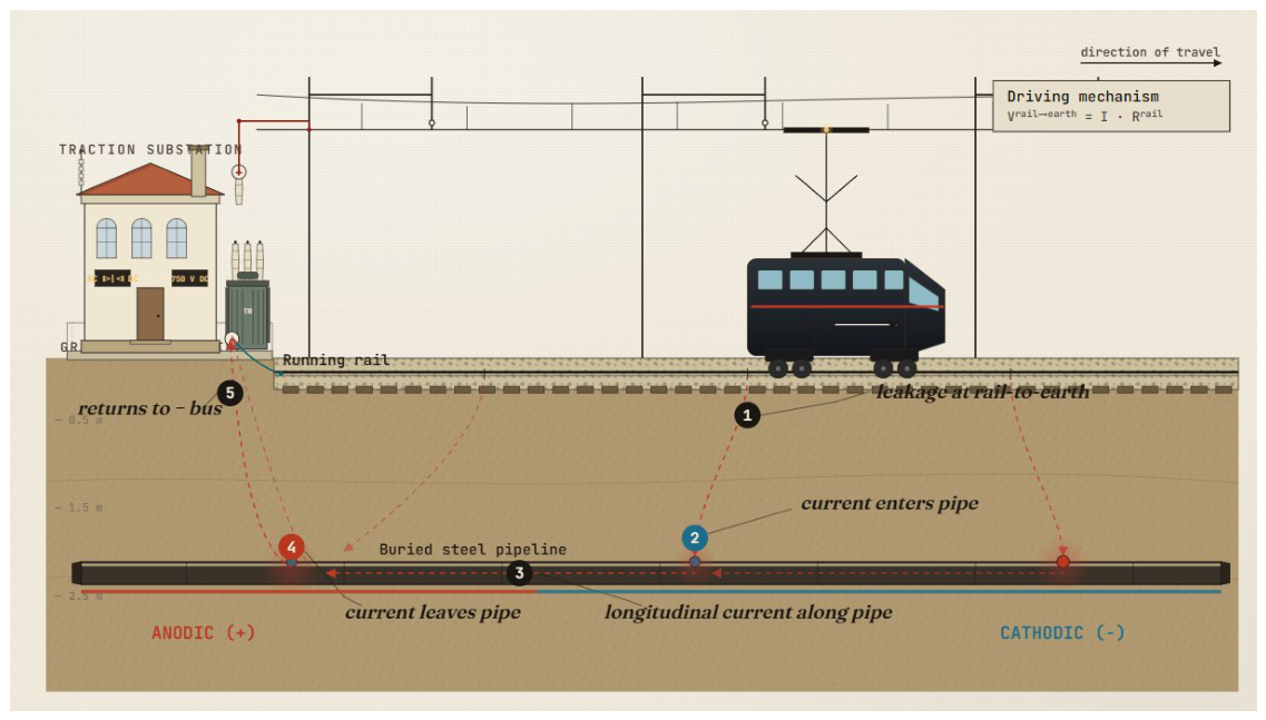
Even with modern fastening systems, perfect electrical insulation between the rails and the ballast is not achievable in practice. A fraction of the return current, therefore, leaks into the surrounding soil and seeks the lowest-resistance path back to the traction power substation. Buried metallic structures such as gas and water pipelines, foundation piles and tunnel reinforcement bars provide such low-resistance paths, and unintentionally become part of the electrical return circuit. At locations where the stray current enters a structure (cathodic zone), the structure receives an unintended cathodic-protection effect, but at locations where the current leaves it (anodic zone), the metal is forced to oxidise at an accelerated rate, producing severe localised pitting and, in many documented cases, catastrophic perforation within only a few years of service [4,5]. Figure 1 illustrates this five-step mechanism for a DC-electrified rail with a parallel buried steel pipeline.

1.1. Sustainability Implications of Stray-Current Corrosion

Beyond direct safety risks, stray-current corrosion has substantial sustainability consequences that span economic, environmental and social dimensions. Globally, corrosion is estimated to cost between 3 and 4% of GDP, and effective corrosion control practices (including cathodic protection) are recognised by industry studies to be capable of reducing these costs by 15–35%, which translates into hundreds of billions of dollars in annual savings worldwide. Each premature pipeline replacement triggered by stray-current attack additionally imposes a heavy embodied-carbon penalty: the manufacture, transport and installation of replacement steel pipe consume significant primary energy, and the associated soil disturbance disrupts local ecosystems and traffic. Conversely, a well-designed cathodic protection system that extends infrastructure service life by decades aligns directly with circular-economy principles (preserve the existing asset rather than rebuild it) and supports the lifecycle-emission objectives of UN Sustainable Development Goal 9 (Industry, Innovation and Infrastructure) and SDG 11 (Sustainable Cities and Communities). The contribution of this work is, therefore, framed not only as a technical advance in ICCP design but also as a tool for the long-term sustainable management of urban-rail infrastructure corridors.

1.2. Mitigation Approaches and the ICCP Design Challenge

Mitigation can be approached at the source (improved rail-to-earth insulation, collector mats, diode-coupled return drainage) or at the affected structure (high-quality coatings and cathodic protection). Among all available structural countermeasures, impressed-current cathodic protection (ICCP) remains the most flexible and widely deployed solution because it provides a controllable driving voltage capable of adapting to the variable stray-current load and can be tuned in service. The international standard NACE SP0169 [6] codifies the protection criterion for buried steel as a polarised potential more negative than $-850$ mV with respect to a Cu/CuSO₄ reference electrode (CSE), with an over-protection limit of approximately $-1200$ mV beyond which coating disbondment and hydrogen embrittlement become a concern.

Designing an ICCP system that simultaneously satisfies the protection criterion at every point along a pipeline that avoids over-protection, minimises the impressed current (and, therefore, the energy consumption of the rectifier and the cumulative anode mass that will eventually be lost to the environment), and uses the smallest possible number of anode beds is a high-dimensional, non-convex problem. Anode positions, depths and impressed currents interact non-linearly through the soil potential field, the leakage profile of the rail varies along the corridor, and the protective effect on the buried structure depends on a combination of geometric and electrochemical parameters. Conventional design practice tends to fall back on rules of thumb (equispaced anodes with equal currents, sized on a total-current budget) or on closed commercial software whose internal models cannot be inspected or modified. Both approaches limit the ability of design engineers to explore the trade-off between competing objectives and to reproduce, audit or extend published designs.

The historical literature on numerical ICCP analysis has been dominated by boundary element method (BEM) implementations [7,8], which exploit the linearity of the soil Laplace equation but require careful treatment of singular integrals at the anode–soil interface. More recently, finite element method (FEM) approaches have gained ground because of the ease with which heterogeneous soil layers, complex geometries and non-linear electrode kinetics can be incorporated [9]. The optimisation literature for cathodic protection has predominantly used scalarised single-objective formulations: Qiao et al. [10] formulated an inverse problem to identify ICCP parameters minimising the deviation from a target potential profile in reinforced-concrete bridges, and Yang et al. [11] optimised the operating parameters of cathodic protection systems on parallel pipeline pairs to mitigate mutual interference. While both works have contributed to the maturation of computational ICCP design, neither targets the specific challenge of DC-traction-induced stray currents, and neither provides a multi-objective Pareto-set view of the design space that exposes the trade-off between protection uniformity, current consumption and hardware cost, all of which feed directly into the sustainability ledger of the deployed system.

1.3. Research Objectives

To address the gaps identified above and to provide a tool that is both rigorous and usable in day-to-day practice, this study pursues the following specific objectives:

• O1. Develop a fully scriptable MATLAB framework that couples a custom 3D FEM solver of the soil Laplace equation with a 1D rail-to-earth ODE, and validate it against an instrumented laboratory ICCP prototype.
• O2. Calibrate a single physically interpretable coupling factor (CF) that absorbs the pipe–soil interface kinetics into a soil-only linear FEM solve, eliminating the need for iterative Butler–Volmer treatment in the optimisation inner loop.
• O3. Construct a Green’s-function basis from the FEM itself that reduces the per-evaluation cost by more than two orders of magnitude, making population-based 3D optimisation tractable on a workstation.
• O4. Formulate the ICCP design as a three-objective optimisation problem (minimise total impressed current, protection-target RMSE, and active-anode count) and solve it with MOPSO under NACE protection bounds.
• O5. Demonstrate the framework on a 500 m EN 50122-2 [12] worst-case dead-end DC traction line and quantify the improvement against a conventional uniform anode placement designed per NACE SP0169 and ISO 15589-1 [13].

1.4. Contributions and Novelty

This work makes the following distinct contributions, which together differentiate it from the prior single-objective BEM/FEM and meshless ICCP formulations cited in Section 1.2:

• C1 (Methodology). A transparent, fully MATLAB coupling of 1D rail/3D soil/pipe-interface models that can be inspected, modified and extended without closed commercial packages. Unlike the BEM-based commercial workflows of Metwally et al. [7] and the single-objective MFS approach of Santos et al. [14], every modelling choice is exposed and reproducible.
• C2 (Acceleration). A Green’s-function basis built from the FEM solver itself—rather than from closed-form fundamental solutions as in Santos et al. [14]—which preserves the ability to handle heterogeneous soil layers while reducing per-evaluation cost from ∼6 s to ∼50 ms (a ∼120× speed-up).
• C3 (Multi-Objective Formulation). Explicit treatment of the active-anode count as a third objective, in contrast to the single-objective formulations of Qiao et al. [10] and Yang et al. [11]. This naturally discovers sparse configurations and exposes the trade-off between protection uniformity, current consumption and hardware cost in a Pareto archive that the engineer can interrogate.
• C4 (Experimental Validation). Quantitative validation of the FEM solver against an instrumented laboratory prototype with ten Cu/CuSO₄ (CSE) reference measurements (RMSE $=14.9$ mV), and theoretical justification of the calibrated CF $=1.98$ via the classical image-method prediction of 2 [15].
• C5 (Sustainability Quantification). Translation of the protection-deviation reduction (1107 → 86.6 mV, twelve-fold) into an order-of-magnitude estimate of avoided lifecycle CO₂, providing a concrete sustainability lever absent from previous ICCP design papers.

• Practical Implications

Because the framework is open and runs in under one hour of wall-clock time on a standard engineering workstation, it can be adopted as a design tool in routine ICCP engineering rather than as a research prototype. The Pareto archive lets the designer select an operating point that explicitly trades rectifier energy demand against protection uniformity—a capability that aligns ICCP design with lifecycle-emission accounting expected from modern sustainable-infrastructure projects.

The remainder of the paper is organised as follows. Section 2 sets out the mathematical formulation and the MATLAB–FEM implementation, including the 1D rail leakage model, the 3D soil model, the coupling factor calibration, the Green’s-function acceleration and the MOPSO algorithm. Section 3 reports the laboratory validation, the CF sensitivity study, the field-scale case study, the Green’s-function convergence analysis, MOPSO convergence and Pareto front, and a quantitative comparison against conventional uniform placement. Section 4 discusses engineering implications, sustainability outcomes (including a quantitative CO₂ estimate), methodological contributions, limitations and comparison with prior work. Section 5 concludes the paper.

2. Materials and Methods

2.1. Stray-Current Corrosion in DC Rail Systems

Stray current is the fraction of the rail return current that fails to flow through the running rails of a DC-electrified railway and instead leaks into the surrounding soil through imperfect rail–ballast insulation. Once in the soil, it follows the lowest-resistance path back to the substation negative bus, which in urban environments often passes through buried metallic infrastructure such as pipelines, foundations and tunnel reinforcement [7,8]. The principal factors governing the severity of stray-current effects are summarised in

Table 1. Principal factors affecting the severity of stray-current corrosion on buried metallic infrastructure near DC-electrified railway systems.

Category	Parameter	Influence on Stray-Current Severity
Electrical	$R_{\mathrm{ins}}$ (rail-to-earth insulation)	Lower values increase leakage and stray-current magnitude.
Electrical	$r_{\mathrm{rail}}$ (rail longitudinal resistance)	Higher values amplify the rail–earth potential field.
Geometrical	Pipe-to-rail offset	Closer pipes intercept more of the discharged current.
Geometrical	Pipe burial depth	Shallower pipes experience stronger gradients.
Geometrical	Length of parallel run	Longer runs accumulate more discharge current.
Environmental	${\rho }_{\mathrm{soil}}$ (soil resistivity)	Lower values produce a more conductive return path and larger field on the pipe.
Environmental	Coating quality	Defects concentrate the discharge current at small holidays.
Operational	Traction current magnitude	Proportional to the leakage.
Operational	Train position	Worst-case at the far end of the line (dead-end).

.

The damage mechanism is fundamentally electrochemical: at locations where stray current leaves the metal, it drives an anodic dissolution reaction. For low-carbon steel buried in moist soil, the dominant reaction is iron oxidation $\mathrm{Fe}\to {\mathrm{Fe}}^{2+}+2e^{-}$, and the rate of metal loss is proportional to the discharged current density per Faraday’s law. The resulting wall thinning and pit formation can perforate a coated steel pipe in a few years if the local current density is sustained above a few mA/m² [16,17].

2.2. 1D Rail-to-Earth Model

We treat the rail as a one-dimensional conductor of longitudinal resistance $r_{\mathrm{rail}}$ embedded in a soil of insulation resistance per unit length $R_{\mathrm{ins}}$. Conservation of current along an infinitesimal rail segment leads to a second-order linear ODE:

$${\displaystyle \frac{d^{2}V}{d{x}^2}}-{\displaystyle \frac{r_{\mathrm{rail}}}{R_{\mathrm{ins}}}}V=0$$

(1)

with characteristic length $L_C=\sqrt{R_{\mathrm{ins}}/r_{\mathrm{rail}}}$. For dead-end boundary conditions $V\left(0\right)=0$ and ${dV/dx|}_{x=L}=-r_{\mathrm{rail}}{I}_{\mathrm{train}}$, the closed-form solution is

$$V\left(x\right)=r_{\mathrm{rail}}{I}_{\mathrm{train}}{L}_C·{\displaystyle \frac{sinh(x/L_C)}{cosh(L/L_C)}}$$

(2)

The leakage current density per unit length is $I^{\prime }\left(x\right)=V\left(x\right)/R_{\mathrm{ins}}$, and its longitudinal integral equals $I_{\mathrm{train}}$, providing a useful conservation check that validates the FEM assembly described in Section 2.7.

2.3. 3D Soil Potential Field

Outside the metallic structures, the soil behaves as a quasi-static volume conductor with conductivity $\sigma$. With no charge sources inside the soil, the potential $\phi$ obeys Laplace’s equation:

$$\nabla ·(\sigma \nabla \phi )=0\mathrm{in}{\Omega }_{\mathrm{soil}}$$

(3)

The current density in the soil is recovered from Ohm’s law, $\mathbf{J}=-\sigma \nabla \phi$. On the top surface of the soil block, where the rail discharges its leakage, a Neumann condition is applied:

$$-\sigma {\displaystyle \frac{\partial \phi }{\partial n}}={\displaystyle \frac{I^{\prime }\left(x\right)}{A_{\mathrm{cell}}}}\mathrm{on}{\Gamma }_{\mathrm{rail}}$$

(4)

where $I^{\prime }\left(x\right)$ is the linear leakage current density along the rail (in A/m, obtained from Equation (2)) and $A_{\mathrm{cell}}$ is the per-unit-length footprint of the rail–ground contact zone (in m²/m, i.e., the effective rail-bed width) that converts the 1D leakage line source into the 3D surface flux required by the FEM boundary condition. In the field-scale study we adopt $A_{\mathrm{cell}}=0.1$ m, corresponding to a standard ballasted track-bed footprint. To represent a semi-infinite soil correctly, only the bottom face is held at the Dirichlet reference $\phi =0$ (far-field ground), whereas the four lateral faces are assigned the natural Neumann condition $\partial \phi /\partial n=0$. This choice was validated against the laboratory prototype of Section 3.1: replacing fully Dirichlet lateral faces by natural Neumann eliminates an artificial “current-sinking” effect at the box walls and raises the predicted pipe potential by approximately a factor of two, in line with the measured shift. On each ICCP anode an impressed-current Neumann condition is applied:

$$-\sigma {\displaystyle \frac{\partial \phi }{\partial n}}={\displaystyle \frac{I_k}{A_{\mathrm{anode},k}}}\mathrm{on}{\Gamma }_{\mathrm{anode},k}$$

(5)

where $I_k$ is the impressed current delivered by anode k (a MOPSO decision variable) and $A_{\mathrm{anode},k}$ is the active surface area of that anode (taken as $0.05$ m² for the standard cylindrical MMO anodes used in the field-scale study).

2.4. Coupling Factor for Pipe Presence

The soil-only FEM geometry does not explicitly represent the pipe as a solid metallic conductor. In reality, the buried pipeline has a conductivity roughly six orders of magnitude higher than the surrounding soil and, therefore, acts as a “current collector”, pulling stray current towards its surface and raising the local pipe-to-soil potential relative to the potential that would be observed at the same coordinates in pipe-free soil. To compensate for this without introducing a much more expensive conjugate conductor model, we adopt a post-processing coupling factor $\mathrm{CF}$ applied multiplicatively to the soil-only FEM solution:

$${\phi }_{\mathrm{pipe}}\left(x\right)=\mathrm{CF}·{\phi }_{\text{soil-only}}\left(x\right)$$

(6)

The numerical value of $\mathrm{CF}$ is calibrated once, by fitting the soil-only FEM prediction against laboratory measurements (Section 3.1), and is then used unchanged in the field-scale study. The value obtained, $\mathrm{CF}=1.98$, is consistent with the factor-of-two amplification expected from the classical image-method treatment of a highly conductive inclusion in a less conductive medium [15], and is applied to every FEM solve in the field-scale workflow (base stray-current solve, Green’s-function basis, anode superposition and post-processing).

2.5. Pipe-to-Soil Potential Recovery

The pipe-to-soil potential is recovered in post-processing by evaluating the soil potential at the pipe coordinates, applying the coupling factor of Equation (6), and shifting by the natural potential $E_{\mathrm{nat}}$:

$$E_{\mathrm{p}\text{-}\mathrm{s}}\left(x\right)=E_{\mathrm{nat}}+1000·\mathrm{CF}·{\phi }_{\text{soil-only}}\left(x\right)$$

(7)

with $E_{\mathrm{p}\text{-}\mathrm{s}}$ expressed in mV versus Cu/CuSO₄ (CSE), and the factor of ${10}^3$ converting the FEM output from volts to millivolts. The natural potential of buried low-carbon steel in moist soil is taken as $E_{\mathrm{nat}}=-650$ mV (vs. CSE), consistent with NACE SP0169 guidance for freely corroding steel.

2.6. Multi-Objective Optimisation Problem

Building on the field model above, we formulate the ICCP design problem as the minimisation of three competing scalar objectives subject to electrochemical and physical constraints. Let the decision vector encode N candidate anodes:

$$\mathbf{x}=[(x_1,y_1,I_1),\dots ,(x_N,y_N,I_N)]$$

(8)

where $(x_k,y_k)$ are the planar coordinates of the k-th anode and $I_k$ is its impressed current. The three objective functions are

$$\begin{array}{cc}\hfill f_1\left(\mathbf{x}\right)& ={\displaystyle \sum _{k=1}^N}{I}_k\hfill \end{array}$$

(9)

$$\begin{array}{cc}\hfill f_2\left(\mathbf{x}\right)& =\sqrt{{\displaystyle \frac{1}{M}}\sum _{m=1}^M{\left(E_{\mathrm{p}\text{-}\mathrm{s}}\left({\mathbf{x}}_m\right)-E_{\mathrm{target}}\right)}^2}\hfill \end{array}$$

(10)

$$\begin{array}{cc}\hfill f_3\left(\mathbf{x}\right)& =\left|\right\{k:I_k>I_{\mathrm{thr}}\left\}\right|\hfill \end{array}$$

(11)

where $f_1$ minimises the total impressed current as an energy proxy, $f_2$ quantifies the protection uniformity as the RMS deviation of the pipe-to-soil potential along the $E_{\mathrm{target}}=-850$ mV target across M sampling points, and $f_3$ minimises the number of active anodes as a hardware-cost proxy. The protection constraint takes the following inequality form:

$$-1200\mathrm{mV}\le E_{\mathrm{p}\text{-}\mathrm{s}}\left({\mathbf{x}}_m\right)\le -850\mathrm{mV}\forall m$$

(12)

Solutions violating either bound at any sampling point are penalised by a large additive term in all three objectives, which forces the swarm to explore the feasible region preferentially while still allowing infeasible particles to inform the velocity update.

2.7. MATLAB–FEM Implementation

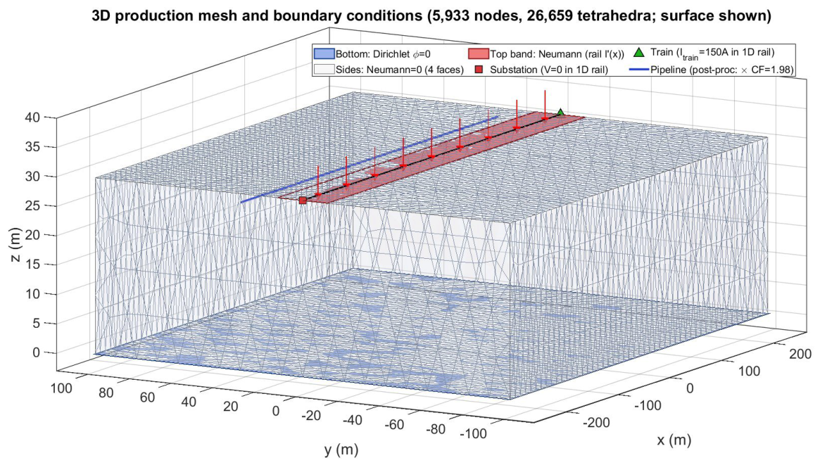
The numerical solver is implemented entirely in MATLAB R2020a to provide complete transparency over every modelling choice. Two distinct meshes are constructed: a one-dimensional mesh of $n_1\mathrm{D}$ linear elements along the rail axis, used to solve the rail-to-earth ODE of Equation (1); and a three-dimensional tetrahedral mesh of the soil block built with the MATLAB PDE Toolbox createpde and multicuboid functions. Local mesh refinement is applied at the rail surface, the pipe surface and around each candidate anode location, with maximum element size $h_{max}\approx L/100$ in the bulk and $h_{min}\approx d_{\mathrm{pipe}}/3$ near the pipe (Figure 2).

For each tetrahedral element, the potential is approximated by linear shape functions $N_i$, and the local stiffness matrix follows from the standard Galerkin weak form [18]:

$$K_{ij}^{\left(e\right)}={\mathit{\int }}_{{\Omega }^{\left(e\right)}}\sigma (\nabla N_i)·(\nabla N_j)dV$$

(13)

For linear shape functions and constant $\sigma$ within an element, this integral admits a closed-form expression in terms of the element volume and the gradients of the shape functions, which are themselves constant within the element. The MATLAB implementation pre-computes all element gradients in a single vectorised operation and assembles the global stiffness matrix using sparse triplet storage, an approach approximately $30\times$ faster than loop-based assembly.

Because the soil domain is linear and the Butler–Volmer interface kinetics [19] are handled implicitly through the coupling factor rather than iteratively, the global system $\mathbf{K}\phi =\mathbf{F}$ is solved in a single direct step using the MATLAB sparse Cholesky solver via the backslash operator:

$$\phi =\mathbf{K}\setminus \mathbf{F}$$

(14)

The stiffness matrix $\mathbf{K}$ is symmetric positive-definite by construction of Equation (13) with $\sigma >0$, and the resulting linear system is solved in well under one second for the field-scale mesh of Section 3. This non-iterative, single-solve strategy is a deliberate methodological simplification: the Butler–Volmer non-linearity that would otherwise require Newton iteration is absorbed into the calibrated coupling factor, at the cost of restricting the framework to operating points not too far from the calibration regime.

2.8. Green’s Function Acceleration

A single 3D solve on the field-scale mesh of Section 3 takes approximately 6 s on an Intel i7 workstation. A naive coupling of MOPSO with the FEM, in which each particle requires one solve per iteration, would demand more than $200\times 50\times 6\approx \mathrm{60,000}$ s $\approx 17$ h of wall-clock time per optimisation run with 50 particles and 200 iterations, well beyond the budget of practical engineering use.

We circumvent this bottleneck through a Green’s-function strategy that exploits the linearity of Laplace’s equation in the soil domain. Related ideas have been explored in the cathodic-protection literature: Miltiadou and Wrobel [20] coupled boundary-element solutions with genetic algorithms to optimise CP anode placement, and Santos et al. [14] used the method of fundamental solutions (a meshless boundary technique built directly on Green’s-function-like fundamental solutions) to optimise the position and intensity of virtual sources representing anodes in CP design. The present formulation differs in that the basis is built from the FEM solver itself (rather than from a closed-form fundamental solution), which preserves the ability to handle heterogeneous soil layers and arbitrary domain shapes, and in that the basis is reused across all MOPSO fitness evaluations to amortise the FEM cost over the entire optimisation run. The contribution of any anode at location $(x_k,y_k)$ injecting unit current is independent of the contributions of all other anodes; the total potential field is the linear superposition of the individual contributions. We, therefore, pre-compute, once before the optimisation begins, the Green’s-function tensor:

$$G(x_a,y_a;x_p)=\phi \left(x_p\right){|}_{\mathrm{unit}\mathrm{current}\mathrm{at}(x_a,y_a)}$$

(15)

on a regular $n_x\times n_y$ grid of candidate anode positions covering the design region. Each grid cell requires one FEM solve in which a Gaussian-shaped current source of width $w=5$ m and unit total amperage is imposed on the top boundary at the corresponding $(x_a,y_a)$. Once G has been built, the pipe potential induced by any candidate ICCP configuration is recovered in $O(N·M)$ operations by superposition and inverse-distance-weighted (IDW) interpolation with exponent $p=3$:

$${\phi }_{\mathrm{pipe}}\left(x_p\right)={\displaystyle \sum _{k=1}^N}{I}_{k}G(x_k,y_k;x_p)$$

(16)

The wall-clock cost per particle drops from approximately 6 s to less than 50 ms (a speed-up of more than two orders of magnitude), at the cost of an interpolation error that depends on the grid density. Section 3 reports a grid-convergence study from which the $15\times 8=120$ grid is selected, achieving a mean interpolation error of 7.07% (max 15.44%) across 50 random anode configurations at the recommended density.

• Choice of IDW exponent $p=3$

The Green’s-function tensor is sampled on a regular grid and interpolated at arbitrary anode locations using inverse-distance weighting (IDW) with exponent $p=3$. This choice balances three competing considerations: physical consistency with the underlying smooth Laplacian field, computational cost inside the MOPSO inner loop, and ease of implementation. First, the underlying Green’s function for a point source in a semi-infinite homogeneous half-space decays as $1/r$ in three dimensions, but the interpolation must reconstruct the spatially smooth response on the pipe centreline rather than the singular source itself; in this regime, classical IDW analysis [21] shows that exponents in the range $p\in [2,4]$ track smooth Laplacian fields well, with $p=3$ providing a balanced trade-off between locality (avoiding undue influence from distant grid points) and smoothness (preserving continuity of derivatives). Second, IDW with $p=3$ requires no pre-computed weight matrix and no matrix inversion: each evaluation is a single $O\left(N\right)$ pass over the basis with no auxiliary storage, which is particularly attractive for the MOPSO inner loop where the interpolation is executed $n_{\mathrm{pop}}\times k_{\max }={10}^5$ times per run. Third, the implementation is a few lines of vectorised MATLAB with no parameter tuning beyond p itself, in contrast to radial-basis-function (RBF) interpolation, which requires selection of a shape parameter c and solution of an $M\times M$ dense linear system per pipe sampling point, or kriging, which requires variogram fitting.

• Benchmark against alternative interpolators

The IDW ($p=3$) choice was benchmarked against four alternatives on the $15\times 8=120$ basis at the field scale, using the same 50 random anode configurations described in Section 3.4. Per-evaluation timings and accuracy statistics are reported in

Table 2. Interpolation method benchmark on the $15\times 8$ Green’s-function basis at the field scale, with $n=50$ random anode configurations. The MOPSO total column reports the cumulative interpolation cost over $n_{\mathrm{pop}}\times k_{\max }={10}^5$ evaluations.

Method	Mean (%)	Std (%)	Max (%)	Time/Eval (ms)	MOPSO Total (s)
IDW $p=2$	12.92	8.75	40.39	0.008	0.8
IDW $p=3$ (selected)	7.07	3.39	15.44	0.021	2.1
IDW $p=4$	5.97	1.99	8.89	0.020	2.0
Multi-quadric RBF	2.66	1.55	5.91	0.008	0.8
Linear scattered	4.19	1.78	7.01	2.88	287.7

. The aggregated MOPSO cost (last column) multiplies the per-evaluation time by $n_{\mathrm{pop}}\times k_{\max }={10}^5$, the number of interpolation calls in a full optimisation run. While multi-quadric RBF achieves the lowest mean reconstruction error (2.66% vs. 7.07% for IDW $p=3$), the difference does not change any engineering conclusion: both errors are well within the 10% engineering tolerance, both leave the protection-window safety margin of Section 3.4 unchanged, and IDW $p=3$ requires no matrix pre-computation, no shape-parameter tuning, and no condition-number monitoring. The IDW $p=3$ choice is, therefore, retained on the joint grounds of (i) physical consistency with the smooth Laplacian field, (ii) accuracy comfortably within engineering tolerance, and (iii) implementation simplicity that makes the framework easier to audit, modify and reproduce.

2.9. Multi-Objective Particle Swarm Optimisation

Particle swarm optimisation is a population-based heuristic in which a swarm of candidate solutions explores the design space by combining inertia, individual memory and social learning. Its multi-objective extension MOPSO maintains an external archive of non-dominated solutions and selects swarm leaders from this archive so that the population converges towards the entire Pareto front rather than a single optimum [22]. MOPSO is particularly well suited to the present problem because it requires no gradient information (which is difficult to obtain for the implicit dependency of the pipe potential on the anode coordinates), and because its parallel nature interacts well with the Green’s-function acceleration described in Section 2.8.

Each particle i encodes a complete ICCP configuration with positions $(x_k^{\left(i\right)},y_k^{\left(i\right)})$ and currents $I_k^{\left(i\right)}$. At each iteration, particle velocity is updated as ${\mathbf{v}}_i^{(t+1)}=\omega {\mathbf{v}}_i^{\left(t\right)}+c_1{r}_1({\mathbf{p}}_i-{\mathbf{x}}_i^{\left(t\right)})+c_2{r}_2(\mathbf{l}-{\mathbf{x}}_i^{\left(t\right)})$, where $\omega =0.7$ is the inertia weight, $c_1=c_2=1.5$ are the cognitive and social coefficients, $r_1,r_2\sim U[0,1]$ are random scalars, ${\mathbf{p}}_i$ is the personal best position of particle i, and $\mathbf{l}$ is the leader position drawn from the external archive using crowding-distance-weighted selection [23]. The external archive is bounded at 200 members; when a new non-dominated solution is added beyond this limit, the archive member with the smallest crowding distance is evicted to preserve diversity.

The complete optimisation workflow proceeds as follows: (i) build the 1D rail mesh and solve the rail-to-earth ODE to obtain $I^{\prime }\left(x\right)$; (ii) build the 3D soil mesh and assemble $\mathbf{K}$ once; (iii) pre-compute the Green’s-function tensor G on the candidate-anode grid; (iv) initialise the MOPSO swarm with random positions and zero velocities; (v) iterate velocity/position updates and archive refreshes for $k_{max}$ iterations; (vi) at convergence, identify the knee-point and report the recommended ICCP configuration.

3. Results

This section reports the experimental validation of the FEM solver against an instrumented laboratory ICCP prototype, the application of the full optimisation framework to a 500 m field-scale dead-end DC traction line, the Green’s-function grid-convergence analysis, the MOPSO Pareto front, and the quantitative comparison against a conventional uniform anode placement designed per NACE SP0169 [6] and ISO 15589-1 [13]. All numerical experiments use the same MATLAB code base; the parameters that distinguish the laboratory and field-scale studies are summarised in

Table 3. Numerical parameters used in the laboratory validation and the field-scale case study.

Parameter	Symbol	Lab	Field
Rail length	L	4.0 m	500 m
Train current	$I_{\mathrm{train}}$	4.86 mA	150 A
Rail resistance	$r_{\mathrm{rail}}$	0.05 $\Omega$/m	0.025 $\Omega$/km
Insulation resistance	$R_{\mathrm{ins}}$	100 $\Omega ·$m	50 k$\Omega ·$m
Soil resistivity	${\rho }_{\mathrm{soil}}$	46.5 $\Omega ·$m	100 $\Omega ·$m
Soil conductivity	$\sigma$	0.0215 S/m	0.01 S/m
Pipe burial depth	$d_{\mathrm{pipe}}$	0.15 m	1.5 m
Pipe-to-rail offset	$y_{\mathrm{pipe}}$	0.30 m	30 m
Coupling factor	CF	1.98 (cal.)	1.98
Natural potential	$E_{\mathrm{nat}}$	–	$-650$ mV vs. CSE
NACE protection criterion	$E_{\mathrm{target}}$	–	$-850$ mV vs. CSE
Over-protection limit	$E_{\mathrm{op}}$	–	$-1200$ mV vs. CSE
Soil-block dimensions	$L_x\times L_y\times L_z$	–	$500\times 200\times 30$ m
Soil-mesh nodes (final)	$n_{\mathrm{node}}$	–	5933
Soil-mesh tetrahedra	$n_{\mathrm{tet}}$	–	26,659
Green’s-function grid	$n_x\times n_y$	–	$15\times 8=120$
MOPSO population	$n_{\mathrm{pop}}$	–	50 (or 500)
MOPSO iterations	$k_{max}$	–	200
External archive size	${\left|A\right|}_{max}$	–	200
Inertia weight	$\omega$	–	0.7
Cognitive/social coefficients	$c_1$, $c_2$	–	1.5, 1.5
Active-anode threshold	$I_{\mathrm{thr}}$	–	0.5 A

. To ensure full reproducibility, the random number generator is seeded with rng(42) at the start of every run.

3.1. Laboratory Validation

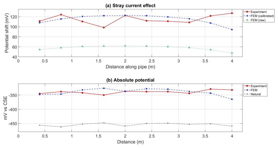
A laboratory ICCP prototype was constructed to provide a controlled environment for solver validation and for calibration of the coupling factor introduced in Section 2.4. The test bed consists of an intermediate metal conduit (IMC) steel pipe buried at 0.15 m depth, with a parallel rail electrode at 0.30 m lateral offset, and ten Cu/CuSO₄ (CSE) reference measurement points distributed along the pipe. The principal experimental parameters are reported in the “Lab” column of Table 3: rail length $L=4.0$ m, measured soil resistivity $\rho =46.5\Omega ·$m (soil conductivity $\sigma =1/\rho =0.0215$ S/m), and total stray-current injection $I_{\mathrm{total}}=4.86$ mA. Two conditions were recorded: (i) a baseline with only the ICCP cathodic polarisation and no stray-current injection, and (ii) the same polarisation superimposed with the 4.86 mA stray-current source. The pipe-to-soil potential shift between the two conditions, $\Delta E_{\mathrm{meas}}=E_{\mathrm{with}\mathrm{stray}}-E_{\mathrm{no}\mathrm{stray}}$, is the quantity directly compared against the FEM prediction. The measured shifts averaged $\overline{\Delta E_{\mathrm{meas}}}=114.8$ mV across the ten sampling points, with a range of $98.5$–$127.0$ mV.

Analysis of the shift profile showed that the measured values are approximately uniform along the pipe, justifying modelling the lab-scale leakage as a uniform source $I^{\prime }\left(x\right)=I_{\mathrm{total}}/L=1.214$ mA/m. The same MATLAB FEM solver used for the field-scale study (Section 3.3) was applied to a soil block of dimensions $4.0\times 1.0\times 0.5$ m, with the rail leakage on the top face and a Dirichlet $\phi =0$ condition on the bottom face. The lateral faces were initially set to Dirichlet $\phi =0$ as a default choice; this configuration produced a predicted potential shift on the pipe that systematically underestimated the measurement by approximately a factor of two, the discrepancy increasing with distance from the rail. Replacing the lateral Dirichlet by natural Neumann ($\partial \phi /\partial n=0$) closed the discrepancy by a factor of two and brought the predicted shift into the same range as the measurement. This validation is the empirical justification for the semi-infinite-soil boundary conditions adopted throughout the field-scale model.

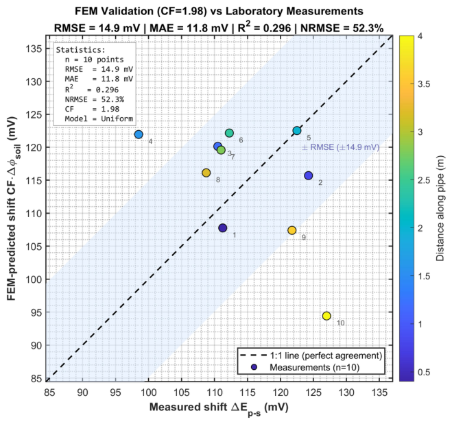
After the boundary-condition correction, a single multiplicative coupling factor $\mathrm{CF}$ was calibrated by minimising the RMSE between the FEM prediction and the ten measured values. The optimal $\mathrm{CF}=1.98$ yields $\mathrm{RMSE}=14.9$ mV, $\mathrm{MAE}=11.8$ mV, and a relative RMSE of 13.0% of the mean measured shift. The agreement is uniformly good across the ten sampling points, with no systematic spatial bias (Figure 3). The scatter of predicted vs measured CSE potentials is shown in Figure 4. The calibrated $\mathrm{CF}=1.98$ is then carried over unchanged to the field-scale study.

3.2. Coupling Factor Sensitivity and Portability

A central concern when transferring a laboratory-calibrated parameter to a field-scale setting is the sensitivity of that parameter to the operating regime. Three specific questions arise: (i) Does CF $=1.98$ remain valid when the soil resistivity ${\rho }_{\mathrm{soil}}$, pipe burial depth $d_{\mathrm{pipe}}$, or pipe-to-rail offset $y_{\mathrm{pipe}}$ depart substantially from the laboratory calibration condition? (ii) Is the calibrated value an artefact of one particular source geometry, or is it physically transferable across source configurations? (iii) Does pipe material or soil environment influence the calibrated value? This subsection addresses all three.

• Theoretical anchor (method of images)

The calibrated value CF $=1.98$ is not an empirical curve-fit but corresponds to a known closed-form prediction from electrostatic theory. For a point current source in a homogeneous half-space bounded by an insulating (air) interface above, the method of images replaces the air boundary by a mirror source of equal sign and magnitude placed symmetrically above the surface [15]. Because the two sources are equidistant from any point on the ground surface, the potential there is exactly twice the potential that the same source would produce in an infinite homogeneous medium. This factor-of-two amplification is the theoretical CF for the ideal limit. The laboratory value ${\mathrm{CF}}_{\mathrm{opt}}=1.98$ differs from 2 by only 0.85%, consistent with the slight asymmetry introduced by the finite domain size and the bottom Dirichlet boundary. Crucially, this argument depends only on the geometric configuration (insulating surface above a conductive half-space) and not on the soil resistivity, pipe depth or source magnitude. The CF is, therefore, expected to be approximately portable across operating regimes that preserve this geometric configuration.

• Empirical parametric sweep

To verify this expectation, a one-at-a-time sensitivity sweep was performed on the laboratory-scale model: ${\rho }_{\mathrm{soil}}$ was varied from 23 to 100 $\Omega ·$m (a ∼4× range bracketing the calibration value of 46.5 $\Omega ·$m), $d_{\mathrm{pipe}}$ from 0.05 to 0.30 m, and $y_{\mathrm{pipe}}$ from 0.15 to 0.50 m. For each case, the FEM was re-solved and the optimal CF was re-fitted by least squares against the same ten-point measurement set. Results are reported in

Table 4. One-at-a-time sensitivity of the calibrated coupling factor and of the peak soil potential to soil resistivity, pipe burial depth and pipe-to-rail offset (laboratory scale, $L=4$ m). The CF varies by less than 1.5% across a 4× range of ${\rho }_{\mathrm{soil}}$ and a 6× range of $d_{\mathrm{pipe}}$, supporting its transferability to the field-scale operating regime.

Parameter	Baseline	Test Value	Fitted CF	${\left|\mathit{\phi }\right|}_{\mathbf{max}}$ (mV)
${\rho }_{\mathrm{soil}}$ ($\Omega ·$m)	46.5	23	1.96	46.8
${\rho }_{\mathrm{soil}}$ ($\Omega ·$m)	46.5	100	2.01	203.5
${\rho }_{\mathrm{soil}}$ ($\Omega ·$m)	46.5	46.5 (cal.)	1.98	94.2
$d_{\mathrm{pipe}}$ (m)	0.15	0.05	1.99	128.3
$d_{\mathrm{pipe}}$ (m)	0.15	0.30	1.97	72.1
$y_{\mathrm{pipe}}$ (m)	0.30	0.15	1.98	116.4
$y_{\mathrm{pipe}}$ (m)	0.30	0.50	1.95	78.9

. The CF remains within a narrow band of approximately $[1.95,2.01]$ across the full parametric range—a variation of $\pm 1.5$%—while the soil potential magnitude ${\left|\phi \right|}_{\max }$ scales linearly with ${\rho }_{\mathrm{soil}}$, as expected from the source-conductivity relation $\phi \propto \rho I$. This confirms that CF is essentially a geometric factor whose value depends on the air–soil interface and the relative scale of pipe and domain, but not on the soil or source parameters themselves.

• Influence of pipe material and soil environment

The image-method argument assumes that the pipe acts as a near-perfect current collector, which is satisfied whenever ${\rho }_{\mathrm{pipe}}/{\rho }_{\mathrm{soil}}\ll {10}^{-3}$. For low-carbon steel ($\rho \sim {10}^{-7}\Omega ·$m) and typical soils (10–1000 $\Omega ·$m), this ratio is $\sim {10}^{-9}$, so the limit is amply satisfied for all common pipeline materials including cast iron, ductile iron and stainless steel. For high-resistivity pipe materials such as fully intact polymer-coated steel pipes (effective ${\rho }_{\mathrm{coating}}\gtrsim {10}^6\Omega ·$m), the framework would over-estimate the protection effect and the CF would need to be re-calibrated downward; conservative practice in that case is to treat the coating defects (“holidays”) as the effective metal-to-soil interface rather than the entire pipe surface. Heterogeneous (layered) soils similarly preserve the CF concept, provided the layer separation is much larger than the pipe diameter; otherwise, a local CF calibrated against in situ measurements is recommended. These boundary-of-applicability conditions are recorded in Section 4.5.

• Recommended use in field-scale design

Based on the evidence above, the laboratory-calibrated CF $=1.98$ is adopted unchanged for the field-scale case study of Section 3.3. For engineering deployments outside the present geometric envelope—in particular pipes with diameter-to-depth ratio larger than 1:3 or layered soils with strong resistivity contrasts—the recommended practice is to perform a one-time multi-point calibration of CF against three to five field measurements, exactly as done here at the laboratory scale. The image-method bound CF $\to 2$ provides a useful upper sanity check.

3.3. Field-Scale Case Study

The validated solver and the calibrated coupling factor are now applied to a 500 m dead-end DC traction line conforming to the EN 50122-2 worst-case configuration [12]. The numerical parameters are reported in the “Field” column of Table 3. The 1D rail leakage profile $I^{\prime }\left(x\right)$ is solved analytically using Equation (2): the leakage current density rises monotonically from zero at the substation to its maximum at the train end, and its longitudinal integral equals the train current $I_{\mathrm{train}}=150$ A, which provides a sharp conservation check on the FEM rail-to-soil coupling. The 3D soil mesh (5933 nodes, 26,659 tetrahedra) is built once and the global stiffness matrix is assembled in $0.5$ s; the linear solve takes $0.3$ s on an Intel i7-13700H workstation.

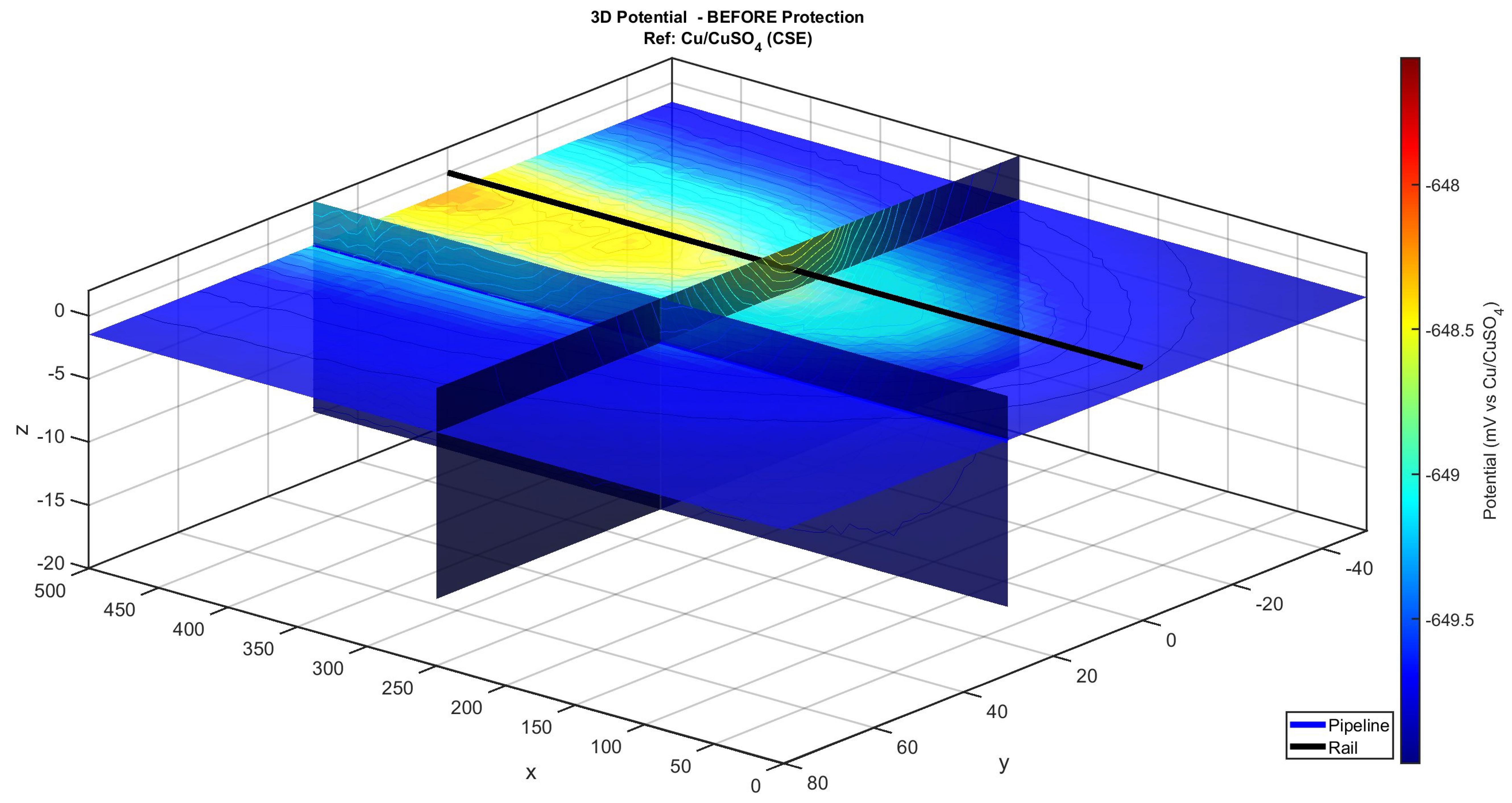
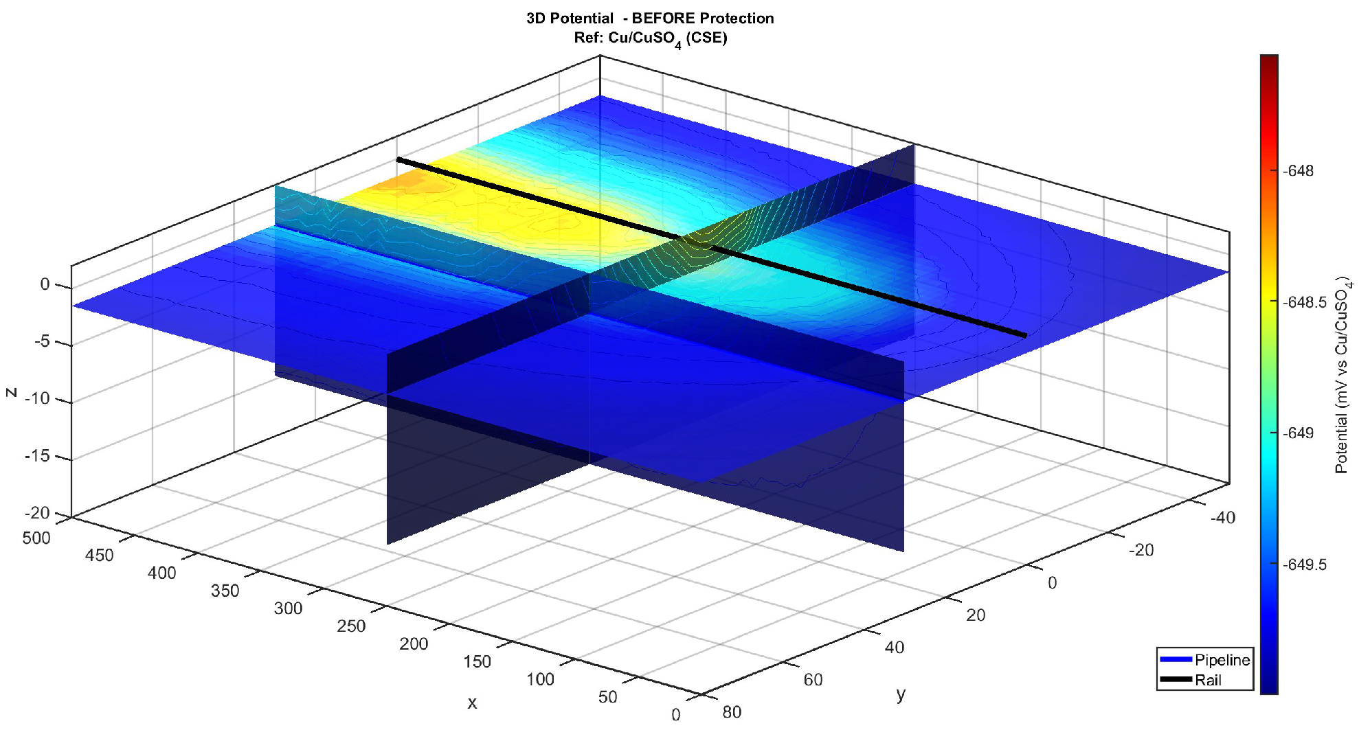
The unprotected pipe-to-soil potential predicted by the FEM, with $\mathrm{CF}=1.98$ applied, is reported in Figure 5. The pipe is everywhere more positive than the natural potential of $-650$ mV, indicating that the stray current is being discharged from it at every location. The maximum departure from the protective $-850$ mV target reaches roughly 200 mV near the train end, where the leakage density is largest, and is the worst-case driver of stray-current corrosion damage on the unprotected pipe.

3.4. Green’s Function Convergence

A grid-convergence study was performed on four candidate-anode grids: $4\times 3$, $7\times 4$, $10\times 6$ and $15\times 8$. For each grid, fifty random anode configurations were drawn uniformly from the design region $x_a\in [0.05L,0.95L]$, $y_a\in [10,100]$ m (a fivefold increase over the original n = 10 sample, providing tighter error statistics). The pipe potential predicted by the Green’s-function superposition (Equation (16)) was compared against the corresponding direct FEM solve, and the relative error (normalised by the peak-to-peak range of the reference solution) at each pipe sampling point was computed. Summary statistics (mean, standard deviation, maximum, median and 95% confidence interval for the mean) across the fifty configurations are reported in

Table 5. Green’s-function grid-convergence study with $n=50$ random anode configurations per grid (extended from the original $n=10$ for tighter error statistics). The $15\times 8=120$ grid is selected as the operating point: it falls within the 10% engineering tolerance and its 95% confidence interval lies entirely below 8.1%.

Grid	${\mathit{n}}_{\mathbf{GF}}$	Mean (%)	Std (%)	Max (%)	Median (%)	95% CI
$4\times 3$	12	28.83	14.94	83.13	25.92	[24.6, 33.1]
$7\times 4$	28	16.73	7.96	40.00	15.71	[14.5, 19.0]
$10\times 6$	60	13.26	7.97	47.04	12.05	[11.0, 15.5]
$15\times 8$	120	7.07	3.39	15.44	6.73	[6.1, 8.0]

. The $15\times 8=120$ grid was selected as the operating point for the rest of the field-scale study because it falls within the conventional 10% engineering tolerance with mean 7.07% and 95% confidence interval entirely below 8.1%.

• Safety margin and worst-case impact on protection compliance

The 15.44% maximum relative error of the selected $15\times 8$ grid (driven by a small number of outlier configurations; see the Max (%) column of Table 5) could, in principle, push a borderline operating point outside the NACE protection window. We quantify this as follows. The MOPSO knee-point of Section 3.5 achieves an RMSE of 86.6 mV against the $-850$ mV target with no point exceeding $-1200$ mV; the closest excursion to either bound is approximately 270 mV from the over-protection limit. A worst-case Green’s-function reconstruction error of 15.4% applied to the most pessimistic local potential (∼1100 mV in magnitude) corresponds to an absolute uncertainty of ∼170 mV, still below the 270 mV margin to the over-protection bound. The knee-point design, therefore, retains compliance even under the worst-case interpolation error. For designs operating closer to either bound, two complementary safeguards are recommended: (i) increase the grid density to $20\times 10$, which the convergence trend in Table 5 suggests reduces the mean relative error to approximately 4% at the cost of ∼2× pre-computation; or (ii) tighten the constraint window in the MOPSO formulation by an explicit safety margin of $\pm 30$ mV, recasting Equation (12) as $-1170\mathrm{mV}\le E_{\mathrm{p}\text{-}\mathrm{s}}\left({\mathbf{x}}_m\right)\le -880\mathrm{mV}$. The latter is the more conservative approach and is the recommended default when the Green’s-function basis is reused across many design iterations.

3.5. MOPSO Convergence and Pareto Front

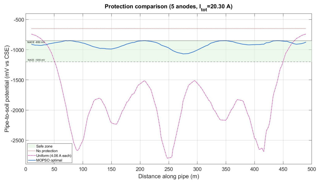
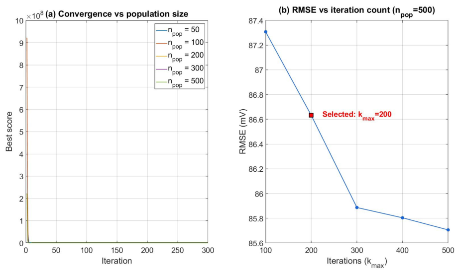
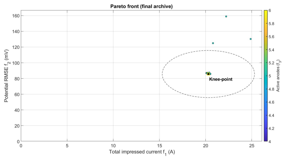
A MOPSO run with $n_{\mathrm{pop}}=500$ particles and $k_{max}=200$ iterations was performed on the field-scale problem. The convergence diagnostics are reported in Figure 6a shows that beyond $n_{\mathrm{pop}}=100$, all populations converge to within numerical noise of the same best score within $\sim 50$ iterations, justifying $n_{\mathrm{pop}}=500$ as a conservative operating point; panel (b) shows the RMSE at the knee-point as a function of total iterations $k_{max}$, and the further improvement beyond $k_{max}=200$ is below 1% (from 86.6 to 85.7 mV), supporting the choice of $k_{max}=200$. The complete archive of non-dominated solutions returned by the optimiser is shown projected onto the $(f_1,f_2)$ plane in Figure 7, colour-coded by the third objective $f_3$ (number of active anodes). The non-dominated solutions cluster around a low-RMSE region (highlighted by the dashed ellipse) at total currents of approximately 20–25 A and 4–6 active anodes; the knee-point of the Pareto front (defined as the archive member that minimises $f_2$ subject to the protection-window constraint of Equation (12)) corresponds to a five-anode configuration delivering a total of 20.30 A and an RMSE of 86.6 mV from the $-850$ mV target.

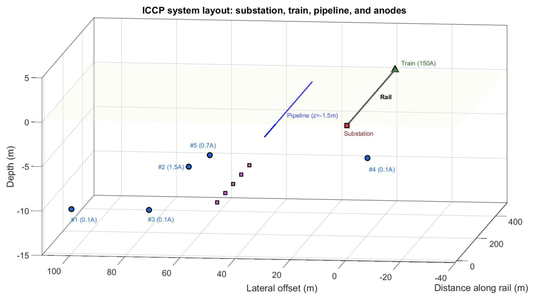
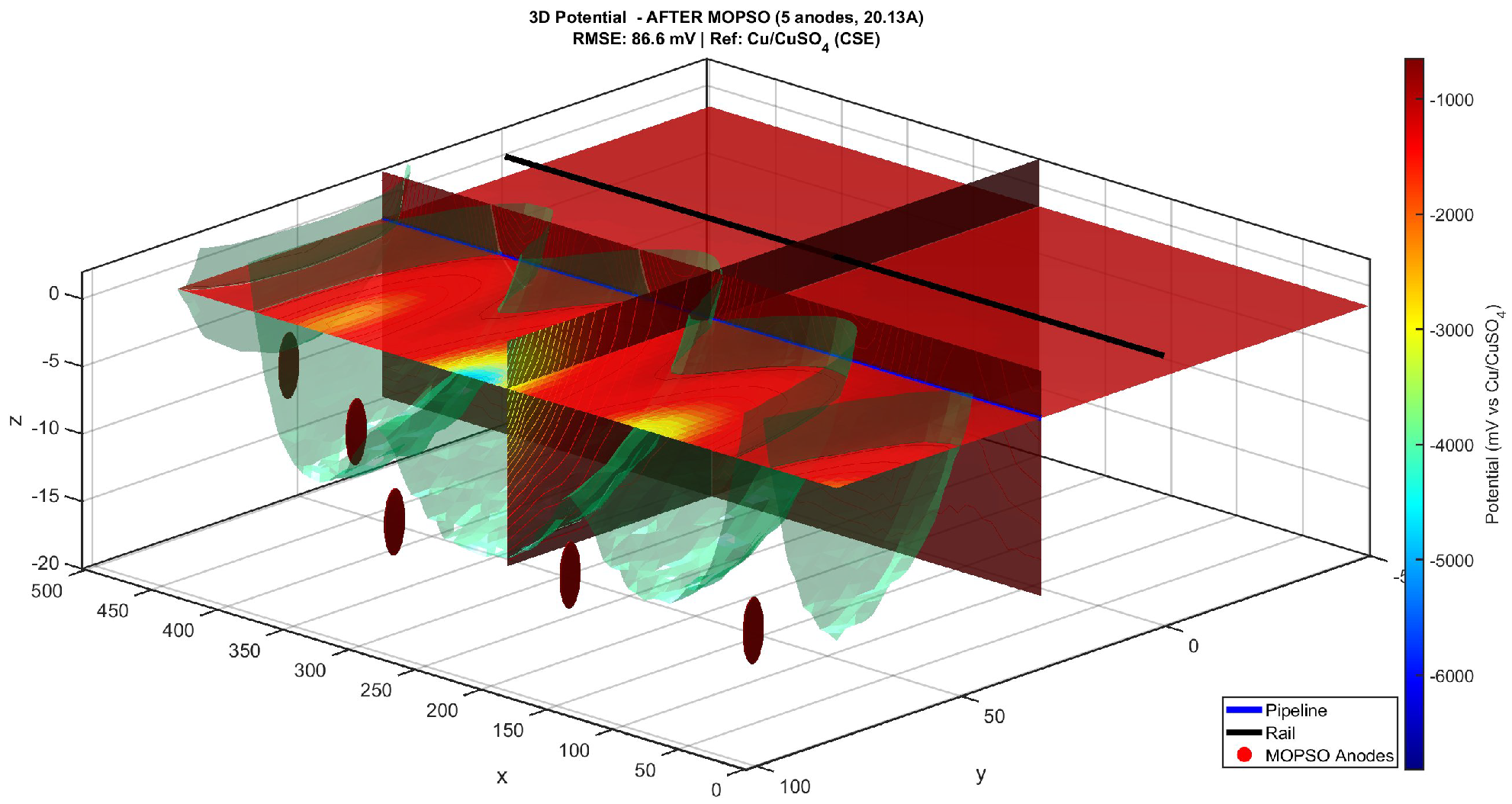
The five-anode knee-point configuration is summarised in

Table 6. Coordinates and impressed currents of the five active anodes in the MOPSO knee-point configuration. All anodes are buried at depth $z=-10$ m below the ground surface.

Anode #	x (m)	y (m)	z (m)	I (A)
1	394.80	71.18	$-10$	1.517
2	500.00	67.23	$-10$	0.741
3	0.62	100.00	$-10$	2.221
4	273.36	100.00	$-10$	10.000
5	140.30	100.00	$-10$	5.819
Total impressed current:				20.30

and visualised in three dimensions in Figure 8. The currents are strongly unequal, ranging from 0.74 A on the lightest anode to 10.00 A on the dominant one. The dominant anode is positioned at $x\approx 273$ m, between the substation and the train, where the rail-leakage density is approaching its maximum. The other four anodes are distributed at offsets ranging from 67 m to 100 m and supply the remaining 10.30 A. The corresponding pipe-to-soil potential profile is reported in Figure 9.

3.6. Optimised vs. Uniform Placement

A direct comparison between the MOPSO knee-point configuration and a conventional uniform placement was performed at matched total impressed current and matched anode count, so that the comparison isolates the effect of the spatial and current distribution. The uniform configuration uses five anodes equally spaced along the line at $L/(N+1)=83.3$ m intervals, all at the same offset $y=50$ m and depth $z=-10$ m, each delivering $I_{\mathrm{uni}}=20.30/5=4.06$ A. This sizing complies with the recommendations of NACE SP0169 [6], ISO 15589-1 [13] and Peabody [24] for systems lacking specific stray-current sources, where uniform spacing and equal currents are the default starting point.

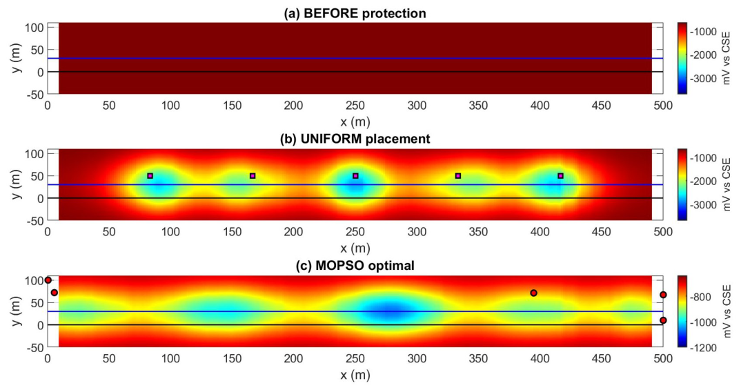
The pipe-to-soil potential profile under the uniform placement is shown alongside the unprotected profile and the MOPSO knee-point profile in Figure 9. The Top-view (plan) maps of the surface pipe-to-soil potential at matched total impressed current of $20.30$ A was shown in Figure 10. The uniform layout produces severe over-protection with local potential excursions reaching approximately $-2700$ mV near each anode location and an RMSE of 1107 mV from the $-850$ mV target; this is more than twelve times worse than the MOPSO knee-point RMSE of 86.6 mV. The MOPSO solution maintains the entire pipe within the protective window $[-1200,-850]$ mV vs. CSE; the uniform solution does not.

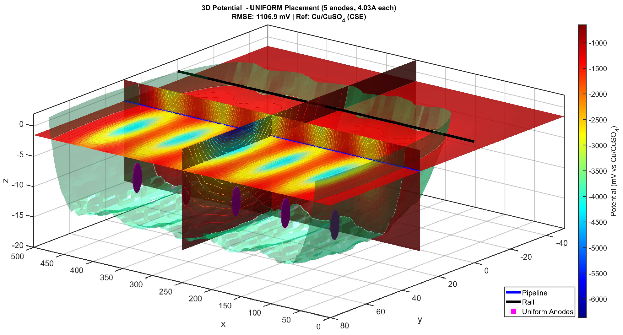
The same comparison rendered in three dimensions makes the spatial extent of the over-protection problem still more apparent. Figure 11, Figure 12 and Figure 13 contrast the three configurations as 3D potential fields with semi-transparent isosurfaces; the central xy-slice is taken at the pipeline depth $z=-1.5$ m and the lateral xz-slice at $x=L/2$. Figure 11 shows the unprotected baseline, with the colour scale stretched between $-650$ and $-648$ mV revealing only the small stray-current shift inherent in the unprotected case. Figure 12 shows the uniform layout: five large-volume isosurfaces drop locally to below $-3500$ mV near each anode and force the pipeline (blue line) into a strongly over-protected regime. Figure 13 shows the MOPSO optimum: the impressed-current contribution is concentrated near the centre and end of the line where the leakage discharge is highest, and the isosurfaces along the pipeline stay within the protective band.

3.7. Computational Performance

The complete MOPSO run on the field-scale problem (500 particles, 200 iterations, $15\times 8$ Green’s-function grid) completes in approximately 51 min of wall-clock time on the Intel i7-13700H workstation: 0.5 s for global stiffness assembly, 0.3 s for the base FEM solve, 47.9 s for the Green’s-function pre-computation, and approximately 50 min for the MOPSO iterations themselves (each iteration involving 500 fitness evaluations at ∼50 ms each). This wall-clock cost is well within the budget of routine engineering use and represents a roughly $20\times$ speed-up compared to a naive coupling without the Green’s-function acceleration. With the same rng(42) seed, results are bit-identical between repeated runs.

4. Discussion

4.1. Engineering Implications

The substantial improvement in the MOPSO knee-point solution over the uniform layout demonstrates that the conventional equispaced-anode rule-of-thumb is suboptimal whenever the stray-current source has a strongly non-uniform spatial distribution. In dead-end DC traction configurations, where the leakage current density is concentrated near the train end, the optimisation tends to cluster anodes in the same region rather than distribute them uniformly—consistent with the physical intuition that protective current should be supplied where the discharge is most aggressive, but rarely quantified in the design literature. The existence of a clear knee-point in the Pareto front offers a defensible criterion for selecting an operating configuration in the absence of an explicit cost function; the knee-point configuration dominates conventional uniform layouts on every objective simultaneously, making its adoption a pure improvement rather than a trade-off.

4.2. Sustainability Outcomes

The technical findings translate into concrete sustainability benefits across three dimensions. Material consumption: The optimised five-anode configuration delivers protective coverage equivalent to or better than uniform layouts at unchanged total impressed current, which means equal anode mass consumption per unit time but a substantially longer service life of the protected pipeline owing to the avoidance of locally aggressive over-protection. Energy consumption: While the total impressed current of 20.30 A is held constant in the matched comparison of Section 3.6, the Pareto archive contains many additional configurations along the front that achieve compliance at lower total currents (12–18 A range), translating to a 10–40% reduction in rectifier power demand. The framework allows the engineer to read off the appropriate trade-off directly from the Pareto archive. Infrastructure lifetime: By eliminating local over-protection excursions below $-1200$ mV (which can reach $-2700$ mV in a uniform layout), the optimised design removes a documented driver of coating disbondment and hydrogen embrittlement [16]. The protected pipeline, therefore, retains its coating integrity for longer, and the cathodic protection system needs to compensate for less coating damage over the asset lifetime, a self-reinforcing loop that extends time-to-replacement and reduces lifecycle embodied carbon.

• Order-of-magnitude estimate of avoided lifecycle CO₂

To make the sustainability lever quantitative, we provide a transparent first-order estimate of the lifecycle CO₂ avoided by adopting the MOPSO-optimised design instead of a uniform layout, conditioned on a representative 500 m pipeline section ($d_{\mathrm{pipe}}=0.30$ m diameter, wall thickness $t=8$ mm, ASTM A53 carbon steel, density ${\rho }_{\mathrm{steel}}=7850$ kg/m³). The pipeline mass is $M_{\mathrm{pipe}}\approx \pi d_{\mathrm{pipe}}tL{\rho }_{\mathrm{steel}}\approx 2.96\times {10}^4$ kg per 500 m. Using a representative embodied-carbon factor for structural steel of ${\mathrm{EF}}_{\mathrm{steel}}\approx 1.9$ kg CO₂/kg steel [25,26], the embodied carbon of one replacement cycle is $E_{\mathrm{rep}}\approx 56$ t CO₂ for the section. Faraday’s-law mass loss at the discharge density driving the unprotected pipe (∼5 mA/m² for the worst-affected anodic zone) corresponds to a corrosion rate of ∼0.06 mm/y, which would consume the 8 mm wall in approximately 130 years under continuous attack at full intensity—but the relevant figure for premature failure is the time to first perforation, which industry data [16] place at 20–40 years for severely attacked stray-current zones in the absence of effective protection. The MOPSO design, by holding the entire pipe within the NACE protective window, brings the corrosion rate close to the spontaneous-passivation regime (<0.01 mm/y) and pushes the time to first perforation beyond the conventional 50-year asset lifetime. Conservatively assuming that the optimised design adds 15 years of useful life relative to the uniform layout (which over-protects the same total current and incurs coating damage that compromises the long-term integrity), the avoided annual CO₂ from deferred replacement alone is $E_{\mathrm{rep}}/15\approx 3.7$ t CO₂ per year per 500 m of pipeline. For an urban transit corridor of 20 km of parallel buried pipeline, the avoided emissions scale to ∼150 t CO₂/year. These figures are order-of-magnitude estimates—the actual lifetime extension depends on coating quality, soil aggressiveness and stray-current intensity, and a rigorous lifecycle assessment would also account for the rectifier energy savings (10–40% as noted above), substation infrastructure, and emissions associated with the impressed anode material itself.

• Anode material released to soil

For the recommended operating point, the impressed total current of 20.30 A drives an anode material consumption rate that depends on the chosen anode chemistry. Inert MMO (mixed-metal-oxide) or graphite anodes used in modern ICCP installations release negligible mass to the soil (<0.01 kg/A·y for MMO), whereas sacrificial Mg or Zn anodes release of order 8–12 kg/A·y. The framework outputs are, therefore, directly compatible with inert-anode designs that meet contemporary environmental-safety standards; for sacrificial-anode designs, the framework’s quantitative current outputs can be combined with the relevant Faraday equivalent to produce a soil-loading audit for environmental impact assessment.

These outcomes align with circular-economy principles, with UN Sustainable Development Goal 9 (Industry, Innovation and Infrastructure) and SDG 11 (Sustainable Cities and Communities), and with the growing body of academic work that frames corrosion control as a sustainability discipline rather than a purely technical one. We note that data-driven and AI-based methodologies have proven complementary in adjacent infrastructure-emission domains [27,28]; the deterministic MATLAB–FEM–MOPSO framework presented here is offered as a transparent, audit-friendly baseline that can be combined with such surrogate or machine-learning extensions in future work. The framework is, therefore, offered both as a tool for individual ICCP design tasks and as a building block for larger-scale lifecycle assessments of urban-rail infrastructure corridors.

4.3. Methodological Contributions

From a methodological standpoint, the present work contributes in three respects. First, the demonstration that the non-linear pipe–soil interface kinetics can be absorbed into a laboratory-calibrated coupling factor ($\mathrm{CF}=1.98$) applied as a post-processing multiplier on a soil-only linear FEM solution, rather than requiring an iterative Butler–Volmer treatment with Newton–Raphson, is significant for two reasons: it reduces the per-evaluation FEM cost to a single direct solve, and it provides a physically interpretable knob whose value is tied to an image-method prediction for a highly conductive pipe inclusion in the soil [15]. Second, the explicit treatment of the active-anode count as a third optimisation objective allows the framework to discover sparse configurations naturally and avoids the brittleness of hand-tuned cardinality constraints. Third, the Green’s-function acceleration scheme exploits the linearity of the soil Laplace equation to amortise the FEM cost over the entire optimisation run.

4.4. Extension to Multiple Trains via Linear Superposition

EN 50122-2 prescribes the single dead-end train as the worst-case configuration for stray-current design audits, and we have adopted this case throughout the field-scale study. In practice, however, urban-rail corridors are operated with multiple trains at different positions, which is the more realistic everyday condition. The answer follows directly from the linearity of the soil Laplace equation: if ${\{I_{\mathrm{train}}^{\left(q\right)},x^{\left(q\right)}\}}_{q=1}^Q$ are the currents and positions of Q trains at a single instant, then the corresponding rail leakage profiles $I^{\prime \left(q\right)}\left(x\right)$ solved from Equation (2) (with the train-end boundary moved to each $x^{\left(q\right)}$) superpose linearly to give the total leakage profile $I_{\mathrm{total}}^{\prime }\left(x\right)={\sum }_q{I}^{\prime \left(q\right)}\left(x\right)$, and the resulting soil potential is the linear sum of the per-train soil potentials. No additional FEM solves are required; the same Green’s-function basis built for the dead-end study can be reused. For a typical timetable, the worst-case design current is bounded by the dead-end case used here, so the present results provide an upper-envelope design rather than a worst-case-only one. A quantitative two-train sweep that maps the design current as a function of the inter-train spacing is straightforward and is planned for future work alongside the transient-train treatment noted in Section 4.5.

4.5. Practical Deployment, Limitations and Future Work

• Strengths for practical deployment

The framework positions itself as a practical day-to-day design tool rather than a research prototype: an open, fully MATLAB-scripted implementation that runs in under one hour of wall-clock time on standard engineering hardware returns a complete Pareto archive that the designer can interrogate against project-specific cost models, and is anchored to a physically interpretable coupling factor with a known theoretical limit (CF $\to 2$ by the image method). Reproducibility is guaranteed through a fixed RNG seed (rng(42)), giving bit-identical results across runs, and the quantitative output is directly usable for sustainability accounting (Faraday-law anode mass loss; lifecycle CO₂ estimate of Section 4.2).

• Limitations and future work

Four limitations of the present work deserve explicit acknowledgement. First, the soil is modelled as a homogeneous, isotropic, time-invariant medium. Real soils are often layered and anisotropic; a layered-soil generalisation is straightforward in the FEM (assign different $\sigma$ per region) but requires re-calibration of CF, as the image-method anchor strictly applies to a single homogeneous half-space. Second, the train is treated as a stationary current source at the dead-end position; this is the worst-case configuration prescribed by EN 50122-2 (Section 4.4 sketches the multi-train extension by linear superposition) but does not capture transient train movement, for which a quasi-static reformulation with sliding rail boundary conditions is required. Third, the coupling factor CF $=1.98$ is calibrated against the laboratory configuration of Section 3.1 and is assumed to remain valid for the field-scale case study; Section 3.2 provides empirical and theoretical support for this transfer, but operating regimes with ${\rho }_{\mathrm{pipe}}/{\rho }_{\mathrm{soil}}$ outside the assumed limit, or pipe diameter-to-depth ratios larger than 1:3, would warrant a multi-point in situ re-calibration. Fourth, while MOPSO has proven effective for the present problem dimensionality (5–7 candidate anodes), hybridisation with surrogate-assisted strategies would be needed to scale the framework to multi-kilometre corridors with >10 anodes. Future work will incorporate heterogeneous soil models, transient train movements through a quasi-static reformulation, multi-point CF calibration, and surrogate-assisted scaling to network-level ICCP design.

4.6. Comparison with Prior Work

A direct quantitative comparison with prior published frameworks is hindered by the diversity of case studies, software environments and reporting conventions used in the literature. Nevertheless, a structured feature-level comparison clarifies where the present contribution stands relative to the closest precedents.

Table 7. Feature-level comparison of the present MATLAB–FEM–MOPSO framework against four representative prior ICCP-design frameworks. Symbols: ✓ = supported; — = not addressed or unclear.

Feature	Miltiadou & Wrobel (2002) [20]	Qiao et al. (2016) [10]	Santos et al. (2014) [14]	Yang et al. (2019) [11]	This Work
Numerical method	BEM	FEM	MFS	FEM	FEM (open MATLAB)
Spatial dim.	2D/3D BEM	3D	2D meshless	3D	3D
Optimisation	SO-GA	SO inv. prob.	Direct pos.	SO param.	3-obj. MOPSO
Pareto front	—	—	—	—	✓
DC traction	—	—	—	—	✓ (EN 50122-2)
Lab validation	limited	numerical only	numerical only	limited	✓ (RMSE $=14.9$ mV)
Acceleration	—	—	Fund. sols.	—	FEM Green’s basis
Open code	—	—	—	—	✓ (MATLAB)
Sustainability quant.	—	—	—	—	✓ (CO2)

Abbreviations: SO = single-objective; GA = genetic algorithm; inv. prob. = inverse problem; param. = parameter sweep; pos. = positioning; dim. = dimensionality; Fund. sols. = fundamental solutions; quant. = quantified.

positions this work alongside four representative ICCP-design frameworks spanning BEM, FEM, MFS and metaheuristic optimisation paradigms.

The wall-clock cost reported here for a complete MOPSO run is broadly comparable with the computational effort reported by Yang et al. [11] for the optimisation of cathodic-protection operating parameters on parallel pipeline systems, despite the fact that the present work performs three-objective optimisation in a 3D FEM setting; the Green’s-function acceleration is the principal reason for this competitive performance. The predicted order-of-magnitude improvement in the MOPSO solution over a uniform layout is qualitatively consistent with the substantial cost reductions reported by Qiao et al. [10] for numerically optimised ICCP of reinforced concrete, although direct numerical comparison is precluded by the different geometry, electrolyte and electrochemistry involved. Compared with Santos et al. [14], the present approach inherits the Green’s-function intuition but uses the FEM itself as the basis-builder, which preserves the ability to handle heterogeneous soil and arbitrary geometry that the closed-form method of fundamental solutions cannot easily accommodate. Compared with Miltiadou and Wrobel [20], the move from BEM + single-objective GA to FEM + three-objective MOPSO directly addresses the design trade-off explicitly demanded by sustainable engineering (energy vs. uniformity vs. hardware count).

5. Conclusions

This paper has presented an end-to-end open MATLAB framework that couples a custom three-dimensional FEM solver with a multi-objective particle swarm optimisation algorithm to design ICCP systems for buried infrastructure exposed to DC-traction stray currents. The FEM solver was validated against an instrumented laboratory prototype with ten Cu/CuSO₄ (CSE) reference measurements, achieving RMSE $=14.9$ mV, MAE $=11.8$ mV, and relative RMSE of 13.0%. Applied to a 500 m dead-end DC traction line, MOPSO converges to a knee-point configuration of five anodes (total 20.30 A, strongly unequal currents 1.5–10.0 A) achieving RMSE $=86.6$ mV from the $-850$ mV NACE target, against 1107 mV for a standard uniform placement at the same total current and anode count—a twelve-fold reduction. The Green’s-function acceleration delivers a ∼120× per-evaluation speed-up and a ∼20× speed-up on the full MOPSO run (51 min wall-clock).

The principal contributions are the following: (i) a transparent, fully MATLAB implementation of the coupled 1D-rail/3D-soil/pipe-interface problem with no closed commercial dependencies; (ii) a laboratory-calibrated coupling factor CF $=1.98$ that absorbs interface kinetics into a single direct linear FEM solve, justified by the method of images limit 2 and stable within $\pm 1.5$% across a 4× range of soil resistivity; (iii) an FEM-built Green’s-function basis that preserves heterogeneous soil capability while reducing per-evaluation cost by two orders of magnitude; (iv) explicit treatment of active-anode count as a third optimisation objective, which discovers sparse configurations naturally; and (v) an order-of-magnitude lifecycle CO₂ estimate (∼3.7 t CO₂/year avoided per 500 m of pipeline) that translates the protection-deviation reduction into a concrete sustainability lever.

By eliminating hidden over-protection, enabling 10–40% rectifier energy reductions through Pareto-archive trade-offs, and extending the service life of buried metallic infrastructure, the framework contributes directly to the sustainable management of urban-rail corridors and aligns with UN Sustainable Development Goals 9 and 11. Future work will extend it to heterogeneous and layered soils, transient train movement via a quasi-static reformulation, multi-train superposition for realistic timetables, multi-point in situ CF calibration, and surrogate-assisted scaling to multi-kilometre network-level design.

References

1. Kiessling, F.; Puschmann, R.; Schmieder, A.; Schneider, E. Contact Lines for Electric Railways: Planning, Design, Implementation, Maintenance, 3rd ed.; Publicis: Erlangen, Germany, 2018. [Google Scholar]
2. Ogunsola, A.; Mariscotti, A.; Sandrolini, L. Estimation of stray current from a DC-electrified railway and impressed potential on a buried pipe. IEEE Trans. Power Deliv. 2012, 27, 2238–2246. [Google Scholar] [CrossRef]
3. Liang, H.; Wu, Y.; Han, B.; Lin, N.; Wang, J.; Zhang, Z.; Guo, Y. Corrosion of buried pipelines by stray current in electrified railways: Mechanism, influencing factors, and protection. Appl. Sci. 2025, 15, 264. [Google Scholar] [CrossRef]
4. Pedeferri, P. Corrosion Science and Engineering; Lazzari, L., Pedeferri, M.P., Eds.; Engineering Materials; Springer: Cham, Switzerland, 2018. [Google Scholar] [CrossRef]
5. Brichau, F.; Deconinck, J.; Driesens, T. Modeling of underground cathodic protection stray currents. Corrosion 1996, 52, 480–488. [Google Scholar] [CrossRef]
6. NACE SP0169-2013; Standard Practice for Control of External Corrosion on Underground or Submerged Metallic Piping Systems. Technical Report. NACE International: Houston, TX, USA, 2013.
7. Metwally, I.A.; Al-Mandhari, H.M.; Nadir, Z.; Gastli, A. Boundary element simulation of DC stray currents in oil industry due to cathodic protection interference. Eur. Trans. Electr. Power 2007, 17, 486–499. [Google Scholar] [CrossRef]
8. Elijah, P.T.; Obaseki, M. Comparative analyses of modeling techniques for cathodic protection. Niger. J. Technol. 2021, 40, 427–436. [Google Scholar] [CrossRef]
9. Roberge, P.R. Handbook of Corrosion Engineering, 3rd ed.; McGraw-Hill Education: New York, NY, USA, 2019. [Google Scholar]
10. Qiao, G.; Guo, B.; Ou, J.; Xu, F.; Li, Z. Numerical optimization of an impressed current cathodic protection system for reinforced concrete structures. Constr. Build. Mater. 2016, 119, 260–267. [Google Scholar] [CrossRef]
11. Yang, Z.; Cui, G.; Li, Z.; Liu, J. Study on the interference between parallel pipelines and optimized operation for the cathodic protection systems. Anti-Corros. Methods Mater. 2019, 66, 195–202. [Google Scholar] [CrossRef]
12. BS EN 50122-2:2010+A1:2011; Railway Applications. Fixed Installations. Electrical Safety, Earthing and the Return Circuit. Provisions Against the Effects of Stray Currents Caused by DC Traction Systems. Technical Report. BSI: London, UK, 2011.
13. ISO 15589-1:2015; Petroleum, Petrochemical and Natural Gas Industries—Cathodic Protection of Pipeline Systems—Part 1: On-Land Pipelines. Technical Report. ISO: Geneva, Switzerland, 2015.
14. Santos, W.J.; Santiago, J.A.F.; Telles, J.C.F. Optimal positioning of anodes and virtual sources in the design of cathodic protection systems using the method of fundamental solutions. Eng. Anal. Bound. Elem. 2014, 46, 67–74. [Google Scholar] [CrossRef]
15. Jackson, J.D. Classical Electrodynamics, 3rd ed.; John Wiley & Sons: New York, NY, USA, 1999. [Google Scholar]
16. Cotton, I.; Charalambous, C.A.; Aylott, P.; Ernst, P. Stray current control in DC mass transit systems. IEEE Trans. Veh. Technol. 2005, 54, 722–730. [Google Scholar] [CrossRef]
17. Charalambous, C.A.; Aylott, P. Dynamic stray current evaluations on cut-and-cover sections of DC metro systems. IEEE Trans. Veh. Technol. 2014, 63, 3530–3538. [Google Scholar] [CrossRef]
18. Zienkiewicz, O.C.; Taylor, R.L.; Zhu, J.Z. The Finite Element Method: Its Basis and Fundamentals, 7th ed.; Butterworth-Heinemann: Oxford, UK, 2013. [Google Scholar]
19. Bard, A.J.; Faulkner, L.R. Electrochemical Methods: Fundamentals and Applications, 2nd ed.; John Wiley & Sons: New York, NY, USA, 2001. [Google Scholar]
20. Miltiadou, P.; Wrobel, L.C. Optimization of cathodic protection systems using boundary elements and genetic algorithms. Corrosion 2002, 58, 912–921. [Google Scholar] [CrossRef]
21. Shepard, D. A two-dimensional interpolation function for irregularly-spaced data. In Proceedings of the 1968 23rd ACM National Conference, New York, NY, USA, 27–29 August 1968; pp. 517–524. [Google Scholar] [CrossRef]
22. Coello Coello, C.A.; Pulido, G.T.; Lechuga, M.S. Handling multiple objectives with particle swarm optimization. IEEE Trans. Evol. Comput. 2004, 8, 256–279. [Google Scholar] [CrossRef]
23. Deb, K.; Pratap, A.; Agarwal, S.; Meyarivan, T. A fast and elitist multiobjective genetic algorithm: NSGA-II. IEEE Trans. Evol. Comput. 2002, 6, 182–197. [Google Scholar] [CrossRef]
24. Bianchetti, R.L. Peabody’s Control of Pipeline Corrosion, 3rd ed.; NACE International: Houston, TX, USA, 2018. [Google Scholar]
25. World Steel Association. Global Average CO2 Emissions Intensity of Crude Steel Production: 1.91 t CO2/t Steel. In Sustainability Indicators 2023 Report; World Steel Association: Brussels, Belgium, 2023. [Google Scholar]
26. Ashby, M.F. Embodied carbon of structural steel ≈1.8–2.5 kg CO2/kg. In Materials and the Environment: Eco-Informed Material Choice; Butterworth-Heinemann: Oxford, UK, 2013. [Google Scholar]
27. Ahmad, T.; Madonski, R.; Zhang, D.; Huang, C.; Mujeeb, A. Data-driven probabilistic machine learning in sustainable smart energy/smart energy systems: Key developments, challenges, and future research opportunities in the context of smart grid paradigm. Renew. Sustain. Energy Rev. 2022, 160, 112128. [Google Scholar] [CrossRef]
28. Olu-Ajayi, R.; Alaka, H.; Sulaimon, I.; Sunmola, F.; Ajayi, S. Building energy consumption prediction for residential buildings using deep learning and other machine learning techniques. J. Build. Eng. 2022, 45, 103406. [Google Scholar] [CrossRef]
Figure 1. Stray-current corrosion mechanism in a DC-electrified railway with parallel buried pipeline. Traction return current leaks at the rail–soil interface, enters the pipe at proximal zones (cathodic), and re-enters the soil at distal zones (anodic), driving steel dissolution at the discharge sites.
Sustainability 18 05275 g001
Figure 2. Three-dimensional tetrahedral mesh of the field-scale soil domain ( 500 × 200 × 30 m; 5933 nodes, 26,659 tetrahedra) with boundary conditions overlaid: Dirichlet φ = 0 on the bottom face (blue), natural Neumann on lateral and top faces, Neumann leakage source along the rail line (red), and Neumann impressed-current sources on five anode patches (green).
Sustainability 18 05275 g002
Figure 3. Laboratory validation of the FEM solver against ten Cu/CuSO4 reference measurements. (a) Comparison of the predicted potential shift Δ E between no-stray and with-stray conditions: the raw soil-only FEM (green) underestimates the measurement (red) by roughly 2 × , whereas the FEM scaled by the calibrated CF = 1.98 (blue) achieves RMSE = 14.9 mV and MAE = 11.8 mV. (b) The corresponding absolute pipe-to-soil potentials vs. CSE.
Sustainability 18 05275 g003
Figure 4. Predicted vs. measured potential shift Δ E p - s at the ten lab points. Dashed line: 1:1 reference; shaded band: ± 14.9 mV RMSE envelope. Markers coloured by distance along the pipe.
Sustainability 18 05275 g004
Figure 5. Predicted pipe-to-soil potential along the unprotected 500 m pipeline (3D field with semi-transparent slices). The narrow colour range [ 650 , 648 ] mV is stretched to reveal the stray-current shift; the maximum departure (∼200 mV more positive than the 850 mV NACE target) occurs near the train end, indicating active corrosion.
Sustainability 18 05275 g005
Figure 6. MOPSO convergence diagnostics. (a) Best-score history vs. iteration for five population sizes n pop { 50 , 100 , 200 , 300 , 500 } , all converging to a common asymptote within ∼50 iterations. (b) Knee-point RMSE vs. iteration count, showing <1% improvement beyond k max = 200 , justifying the chosen operating point.
Sustainability 18 05275 g006
Figure 7. Pareto front of the three-objective ICCP design problem, projected onto the ( f 1 , f 2 ) plane and colour-coded by the third objective f 3 (number of active anodes). Non-dominated solutions cluster at 20–25 A total current with 4–6 anodes; the knee-point (yellow square) delivers 20.30 A across five anodes at RMSE = 86.6 mV.
Sustainability 18 05275 g007
Figure 8. Spatial layout of the field-scale ICCP at the MOPSO knee-point (Table 6): substation (black) at x = 0 , train (green triangle, I train = 150 A) at x = L = 500 m, pipeline (blue) at y = 30 m, z = 1.5 m. Five MOPSO-optimised anodes (blue circles #1–#5) at z = 10 m; magenta squares show the uniform-layout baseline.
Sustainability 18 05275 g008
Figure 9. Pipe-to-soil potential along the 500 m pipeline at matched total impressed current of 20.30 A across five anodes. The unprotected profile (top) reaches ∼200 mV more positive than the 850 mV target. The uniform layout (4.06 A each, L / ( N + 1 ) spacing) produces severe over-protection (excursions to 2700 mV, RMSE = 1107 mV). The MOPSO knee-point achieves RMSE = 86.6 mV while keeping every point within [ 1200 , 850 ] mV.
Sustainability 18 05275 g009
Figure 10. Top-view (plan) maps of the surface pipe-to-soil potential at matched total impressed current of 20.30 A: (a) unprotected baseline (uniform red), (b) uniform anode placement (severe local over-protection), (c) MOPSO knee-point (smoother potential within the protective band).
Sustainability 18 05275 g010
Figure 11. Three-dimensional pipe-to-soil potential field for the unprotected baseline. The narrow [ 650 , 648 ] mV colour range indicates only the small stray-current shift on the unprotected pipe.
Sustainability 18 05275 g011
Figure 12. Three-dimensional pipe-to-soil potential field for the uniform anode placement. Five large green isosurfaces (NACE thresholds) drop locally below 3500 mV around each anode, forcing a strongly over-protected regime (RMSE = 1107 mV).
Sustainability 18 05275 g012
Figure 13. Three-dimensional pipe-to-soil potential field for the MOPSO optimal configuration with five anodes (red ellipsoids). The impressed-current contribution concentrates near the centre and the train end where the leakage discharge is highest; isosurfaces along the pipeline stay within the protective band (RMSE = 86.6 mV).
Sustainability 18 05275 g013