Sustainable On-Road Energy Harvesting: A CFD Study on Wind Turbine System Integrated with Electric Vehicles

Abstract

Electric vehicles (EVs) are playing a crucial role in decarbonising the transportation industry by cutting down on toxic emissions from vehicles. Increasing the range of EVs is still a major hurdle in the widespread adoption of such vehicles, and serious efforts are underway across the globe in order to address this issue. A potential solution to this is the integration of small wind turbines with EVs to extract wind power and help charge the batteries. However, serious efforts in this regard are severely lacking in the published literature. This study aims to bridge this gap through systematic numerical investigations on a drag-based vertical-axis wind turbine (VAWT) installed on top of an EV. Utilising Computational Fluid Dynamic (CFD)-based solvers, the flow fields associated with the turbine are analysed in detail. Instantaneous and average power produced by the turbine have been critically evaluated over its entire operational range and at different vehicle speeds. The results obtained show that the VAWT has a peak power coefficient (Cp) of 0.46 at a tip speed ratio (λ) of 0.55. The average power produced by the VAWT at 30 mph, 50 mph, and 70 mph is about 160 W, 700 W, and 2 kW, respectively.

1. Introduction

Electric vehicles are fast replacing cars with internal combustion engines as a cleaner alternative because they do not emit toxic pollutants into the environment, thus lowering the carbon footprint of the transportation industry. Currently, the range of EVs is the primary concern, considering the time it takes to charge the batteries, especially in winters with internal heating on [1,2,3]. Moreover, the public charging costs are quite high in the UK at the moment, and home charging might not be feasible for many people who own an EV [4,5]. A potential solution to this is installing a small wind turbine on an EV and using the power to charge the batteries. This approach has been shown to produce very small amounts of power while increasing the aerodynamic drag substantially. However, careful design considerations can potentially counteract this, and the turbine power can be essentially used for internal space heating purposes. As cars travel at speeds of 30–70 mph, depending on whether it is city centre travel or on motorways, wind turbines normally do not operate at such high wind velocities. Thus, the operation and performance of wind turbines installed on EVs and operating at high wind speeds need to be rigorously tested.

1.1. Literature Review

A numerical study to extend EVs’ mileage has been conducted by Ferdous et al. [6] using CFD. The main objective of this study is to harness air from the stagnation zone at the front of the vehicle and channel it into ducts so that it flows into two symmetrically placed horizontal-axis wind turbines (HAWTs). The design focuses on minimising the aerodynamic drag that would have been exerted on the vehicle if an external wind turbine were mounted. The turbine has been tested at a constant air velocity of 15 m/s. The numerical results show that each of the wind turbines produces 180 W. An experimental study by Awal et al. [7] investigated a vehicle top-mounted HAWT for power generation. The study uses a stainless-steel fabricated three-bladed HAWT. A Permanent Magnet DC (PMDC) generator was coupled with the wind turbine to convert mechanical energy into electric power. Road tests were carried out at vehicle speeds of 20–80 km/h, while the turbine’s rotational velocity, torque, and power output were recorded. It has been reported that the turbine’s rotational velocity increases linearly with the vehicle speed, going up from 75 rpm to 405 rpm as the vehicle speed increases from 20 km/h to 80 km/h. The torque produced by the turbine increased from 5 Nm to 60 Nm as the vehicle speed increased from 20 km/h to 80 km/h, while the power produced by the turbine increased from 40 W to 190 W. An experimental study was conducted by Fathabadi [8] on a wind turbine installed behind a vehicle’s condenser, with the aim to produce power without affecting the aerodynamics of the vehicle. The 100 W turbine used in the study comprises seven blades and was coupled with a Permanent Magnet Synchronous Generator (PMSG). It has been reported that the EV range increased by 6.4 km when the turbine was installed.

A numerical study was carried out by Goushcha et al. [9], investigating the power generation from a HAWT placed inside a duct passing through the vehicle, similar to the approach adopted by Ferdous et al. [6]. The duct has a constant cross-sectional area till the wind turbine, while downstream, it converts into a diffuser, i.e., a constantly increasing cross-sectional area of the duct, in order to decelerate the flow downstream the turbine. The CFD results obtained show that the freestream velocity of 11 m/s accelerates to 18 m/s within the duct upstream of the turbine. The turbine has been shown to rotate at 350 rad/s, producing a net power of 41 W and a power coefficient of 0.413. Khan et al. [10] carried out an experimental study on an EV integrated with a HAWT to charge the vehicle’s battery. Investigations were carried out at vehicle speeds of 25–90 km/h, while the turbine was placed at different locations on the vehicle: on the bumper, on the roof, and on the bonnet. Similarly to Awal et al. [7], the turbine was coupled with a PMDC generator. It has been reported that the turbine starts to produce power at 25 km/h, which continues to increase as the vehicle speed increases. At the maximum tested vehicle speed of 90 km/h, the overall power output of the turbine was recorded to be 100 W at a power coefficient of 0.285%. A numerical study carried out by El et al. [11] investigated the integration of a three-bladed 500 W HAWT mounted on the bumper of a car. The study analyses whether the overall power output generated from the turbine can offset the additional aerodynamic drag penalties from the turbine. CFD testing carried out considers three models: a basic car model, a model with a circular frontal opening, and a model with the turbine installed in the circular frontal opening. Aerodynamic and energy performance of these models were reported at the car velocity of 27 m/s for a total distance of 100 km covered. The results show that when the turbine is installed on the car, it recovers 5185 kJ and generates 1400 W over the 100 km distance, resulting in a net energy gain of 5.13%.

Analytical studies were carried out by Mekapati and Choudhury [12,13] considering a 410 W HAWT installed at the front of an EV. The study [12] aimed to investigate how the combination of vehicle speed and wind direction influences the power generated by the turbine. Two scenarios were studied: a vehicle speed of 50 km/h and a variable speed representing daily driving, with a daily commute of 90 min. The results show that under tailwind conditions, the range of the EV extends up to 4.87 km. Further investigations on the trip scenarios along with the timings [13] show that long-trip conditions with tailwind recovered up to 1.76 kWh/day, which translates to an additional 13 km of driving range. In comparison, headwind conditions generate an additional 3.7 km of range from 0.5 kWh/day. Numerical investigations were carried out by Zhao et al. [14] on a drag-based vertical-axis wind turbine (VAWT) mounted behind a car’s front grill. The VAWT consists of four blades arranged in two staggered layers with a 90° phase difference in order to improve the efficiency of the VAWT. The blades were designed in a way that they were adjustable, changing the diameter of the turbine based on the vehicle’s velocity. At lower speeds (<12 m/s), the turbine diameter is 120 mm, which reduces to 60 mm as the vehicle velocity increases. The vehicle velocity varies between 10 and 12 m/s. It has been reported that the turbine produces 3.9–7.1 W of power under these operating conditions.

A numerical study carried out by Almahmoud and Karakaya [15] analysed the power and drag characteristics of a multi-bladed VAWT attached to a Tesla Model S. Testing was carried out at 30 m/s car velocity while the turbine was installed (i) on the roof, and (ii) attached to the grille. It has been reported that the drag coefficient of the vehicle is the highest (0.33) when the turbine is installed on the roof. In comparison, the grille-mounted configuration was shown to decrease the drag coefficient to 0.3. It has been reported that the power generated by the turbine is substantially higher when it is installed on the car roof compared to the front grille. As the study has been carried out using a steady-state solver, it cannot be confirmed what the turbine’s time-averaged power generation is. Moreover, it seems that the wake and the ground effects have not been appropriately captured in the study.

1.2. Rationale for This Study

The reviewed studies collectively indicate that vehicle-integrated wind energy systems are primarily constrained by the trade-off between aerodynamic drag and electrical power generation. HAWTs generally produce more power than VATWs but significantly increase the frontal aerodynamic resistance of the vehicle. In contrast, VAWTs have been shown to exhibit lower drag penalties but insufficient power generation for practical applications [16]. Furthermore, most published CFD-based studies employ steady-state modelling approaches, which may not fully capture transient wake interactions and instantaneous power fluctuations associated with rotating wind turbines mounted on moving vehicles. These limitations motivate the present transient CFD investigation of a confined multi-bladed VAWR configuration.

2. Materials and Methods

2.1. Numerical Modelling of the Wind Turbine Installed on Top of a Car

A computational fluid dynamic (CFD)-based solver has been used in the present study to carry out the numerical modelling of the wind turbine installed on the top of a car. The software utilised for this purpose is ANSYS FLUENT, Release 2026 R1 (ANSYS Inc., Canonsburg, PA, USA) which comprises individual modules for pre-processing, solver execution, and post-processing [17,18]. As the pre-processing stage during any CFD-based study consists of geometric modelling and meshing [19,20], the following sub-sections provide details on these aspects.

2.2. Geometric Modelling of the Flow Domain

The geometric modelling approach adopted in the present study comprises four distinct bodies. These are (i) a car, (ii) a drag-based vertical-axis wind turbine, (iii) a turbine casing, and (iv) the surroundings.

Car: Only the top section of a Kia EV 6 is considered here, i.e., the windscreen, roof, and rear screen, in order to keep the computational costs in check. The dimensions of the car are the same as those of a modern EV.

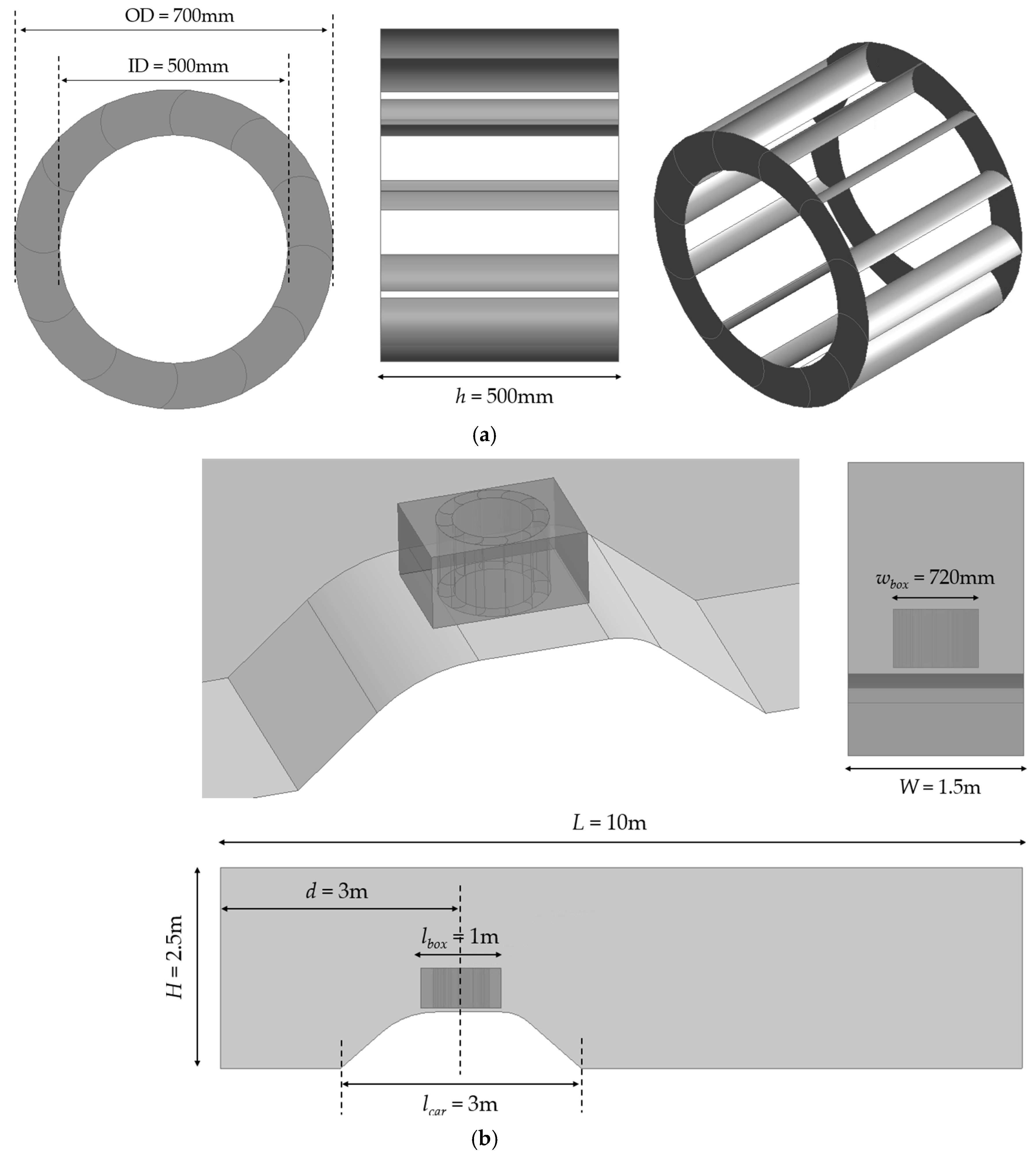
Wind turbine: The drag-based wind turbine used in this study is based on the design developed by Gareth [21]. This wind turbine comprises 12 rotor blades, supported by end plates/rings to hold the blades in place. The blades have a radius of 70.25 mm. The inner and outer diameters of the rotor are 500 mm and 700 mm, respectively, as shown in Figure 1a, while the length of the blades is 500 mm.

Casing: The turbine is placed inside a casing, which is open from both the front and the back to allow airflow through the turbine. This boxed design is safe to use on cars travelling at high speeds, especially in the extreme event of blade loss, where the damage will be contained within the casing. The size of the casing is 1000 mm in length and 720 mm in width, housing a 700 mm diameter turbine in it. The gap between the bottom of the turbine casing and the car roof is 50 mm.

Surroundings: The flow domain around the car is rectangular, with dimensions of 10 m × 2.5 m × 1.5 m (L × H × W). The car and the turbine are placed inside this flow domain such that the middle of the turbine is 3 m from the inlet boundary of the flow domain, as shown in Figure 1b. That leaves 7 m of gap between the turbine and the outlet boundary of the flow domain, which is deemed adequate in this study to analyse the wake of the car and the wind turbine [22].

2.3. Meshing of the Flow Domain

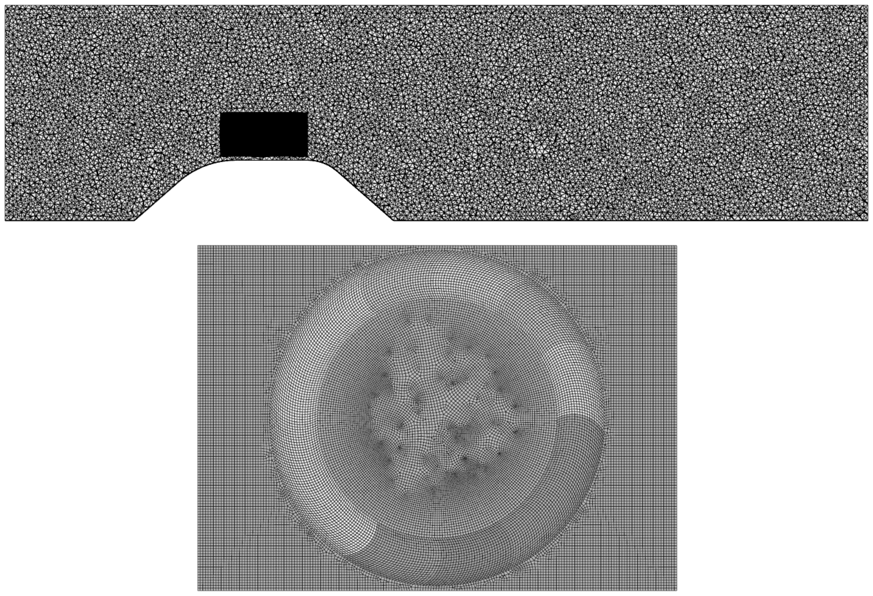
The next stage in CFD after geometric modelling is the spatial discretisation of the flow domain, also known as meshing, which is essentially dividing the flow domain into control volumes in which flow governing equations are solved [23]. Two separate meshing techniques have been utilised in the present study. For the wind turbine and the casing, a structured mesh consisting of hexahedral elements has been generated, while in the surroundings, unstructured tetrahedral elements have been generated [24]. The mesh sizing specified for the wind turbine and the casing is 5.5 mm, while for the surroundings is 60 mm. The resulting mesh consists of 4 million elements and is shown in Figure 2.

2.4. Solver Settings and Turbulence Modelling

A pressure-based segregated solver has been employed in the present study, as the flow velocities associated with cars and wind turbines are typically low. As the flow of air around wind turbines is highly transient in nature, a time-based solver has been chosen for numerical investigations. Three-dimensional Reynolds Averaged Navier–Stokes (RANS) equations are solved iteratively for the turbulent flow of air around the car and across the wind turbine. Air turbulence has been modelled using the 2-equation Shear Stress Transport (SST) k-ω model [25]. The transport equations for the turbulent kinetic energy (k) and the turbulent dissipation rate (ω) are as follows:

$${\displaystyle \frac{\partial }{\partial t}}\left(\rho k\right)+{\displaystyle \frac{\partial }{\partial x_i}}\left(\rho k{u}_i\right)={\displaystyle \frac{\partial }{\partial x_j}}\left[\left(\mu +{\displaystyle \frac{{\mu }_t}{{\sigma }_k}}\right){\displaystyle \frac{\partial k}{\partial x_j}}\right]+G_k-\rho \epsilon -Y_M$$

(1)

$${\displaystyle \frac{\partial }{\partial t}}\left(\rho \omega \right)+{\displaystyle \frac{\partial }{\partial x_i}}\left(\rho \omega u_i\right)={\displaystyle \frac{\partial }{\partial x_j}}\left[{\Gamma }_{\omega }{\displaystyle \frac{\partial \omega }{\partial x_j}}\right]+G_{\omega }-Y_{\omega }$$

(2)

where the first term on the LHS in both equations represents the time derivative, and the second term represents the convection of k and ω. The first term on the RHS is the diffusion term, and G represents the generation of k and ω due to mean velocity gradients. ρε in Equation (1) represents the dissipation of k, while Y_ω in Equation (2) represents the dissipation of ω due to turbulence. Y_M in Equation (1) represents the contribution of fluctuating dilation to the dissipation rate.

The SST k-ω turbulence model has been chosen for numerical investigations in the present study due to its unique transitional feature of switching between a standard k-ω model in the near-wall regions, and a high Reynolds Number (Re) version of the k-ε model in the outer/main flow regions [26]. This feature of the SST k-ω turbulence model allows for more accurate characterisation of separated flows, which are expected in the present study [27].

2.5. Boundary Conditions and Turbine Rotation

Table 1. Boundary conditions.

Body	Boundary	Type	Value
Domain	Left	Velocity inlet (U)	30/50/70 mph
	Right	Pressure outlet	0 Pa,g
	Top, bottom, and sides	Symmetry	-
	Car surfaces	Wall	Stationary/no-slip
Casing	Top, bottom, and sides	Wall	Stationary/no-slip
Wind Turbine	Top and bottom	Wall	Rotating at ω/no-slip
	Blades	Wall	Rotating at ω/no-slip

summarises the boundary conditions used in this study. The domain comprises the velocity inlet and pressure outlet boundaries at either end. Wind speeds of 30/50/70 mph have been tested, mimicking the vehicle speed limit in city centres, on inter-city roads, and on motorways. The outlet boundary is assumed to be far downstream of the car and the turbine, and that the flow has fully recovered. The top, bottom, and sides of the domain are modelled as symmetry, which assumes zero convective and diffusion fluxes across the boundary and zero shear stress at it. Thus, there is zero flux of all quantities across the symmetry, and it can be assumed to be a slip wall. The car surfaces, which are part of the domain body, are modelled as no-slip stationary walls.

The casing of the turbine has been modelled similar to the car surfaces; note that the front and back of the casing are open to flow. The top and bottom (rings) of the turbine are also modelled as no-slip walls, but at a specified rotational speed of the turbine (ω). The blades of the turbine are modelled the same as its top and bottom surfaces. In terms of the rotation of the rotor body (and not just the blades), the Sliding Mesh (SM) technique has been employed in this study, as the focus is to capture transient flow effects and instantaneous power output of the turbine. In this technique, an interface is created between the moving and stationary zones, which, in this study, are the rotor and the casing bodies. As the solution advances in time, node alignment across the interface is not required, which makes this technique easy to implement yet highly accurate in predicting complex flow phenomena at the interface due to the relative motion of the bodies. The rotational velocity of the turbine has been calculated and specified in the solver, depending on the vehicle speed and the tip speed ratio (λ) of the turbine, which can be expressed as follows:

$$\lambda ={\displaystyle \frac{\omega R}{U}}$$

(3)

where ω is the rotational velocity of the turbine in rad/s, R is the radius of the turbine in m, and U is the wind speed incident on the turbine in m/s.

As the wind turbine considered in the present study is a drag-based VAWT, its performance spectrum is normally considered between 0 < λ < 1. This is the same range Gareth [21] also considered while studying this turbine. It has been reported that the λ at which the peak Cp of the turbine has been obtained is 0.3, where Cp is the power coefficient of the turbine, and can be expressed as follows:

$$Cp={\displaystyle \frac{P}{\frac{1}{2}\rho A{U}^3}}={\displaystyle \frac{\omega T}{\frac{1}{2}\rho A{U}^3}}$$

(4)

where P is the power produced by the turbine in watts, T is the torque produced by the turbine in Nm, ρ is the density of air in kg/m³, and A is the swept area of the turbine in m². The swept area of a VAWT is equal to Dh, where D is the diameter of the turbine and h is the height of the turbine, both in m.

2.6. Mesh Independence Testing

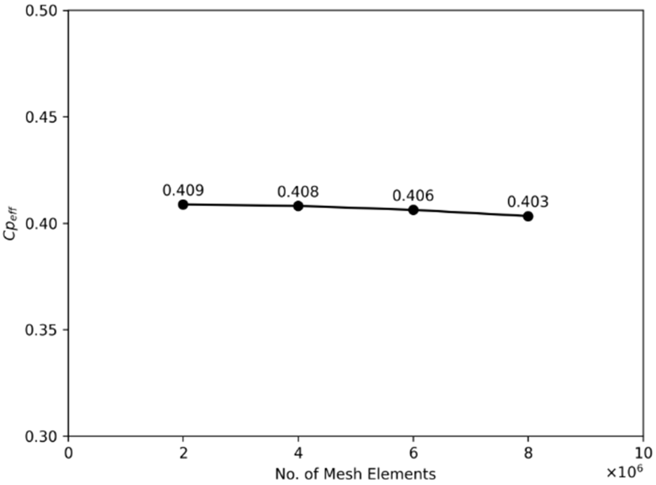
A mesh independence study has been conducted in order to identify the most suitable meshing scheme that appropriately captures the complex flow phenomenon associated with the wind turbine, while keeping the computational cost in check [28]. The effective power coefficient (Cp_eff) has been used to assess the suitability of different meshing schemes considered here. Figure 3 depicts the variations in Cp_eff for four different mesh schemes considered in the present study. These mesh schemes correspond to 2–8 million mesh elements in the flow domain. It can be seen that as the number of elements increases from 2 million to 4 million, Cp_eff decreases by 0.24%. A further increase in the number of mesh elements to 6 and 8 million results in a Cp_eff decrease by 0.5% and 0.74%, respectively. As the difference in Cp_eff between 4 and 8 million elements mesh schemes is negligibly small (1.2%), ensuring that the complex flow behaviour is captured appropriately, especially near the rotor blades and in the wake region, a mesh containing 4 million elements has, therefore, been selected for further numerical investigations.

2.7. Time Step Independence Testing

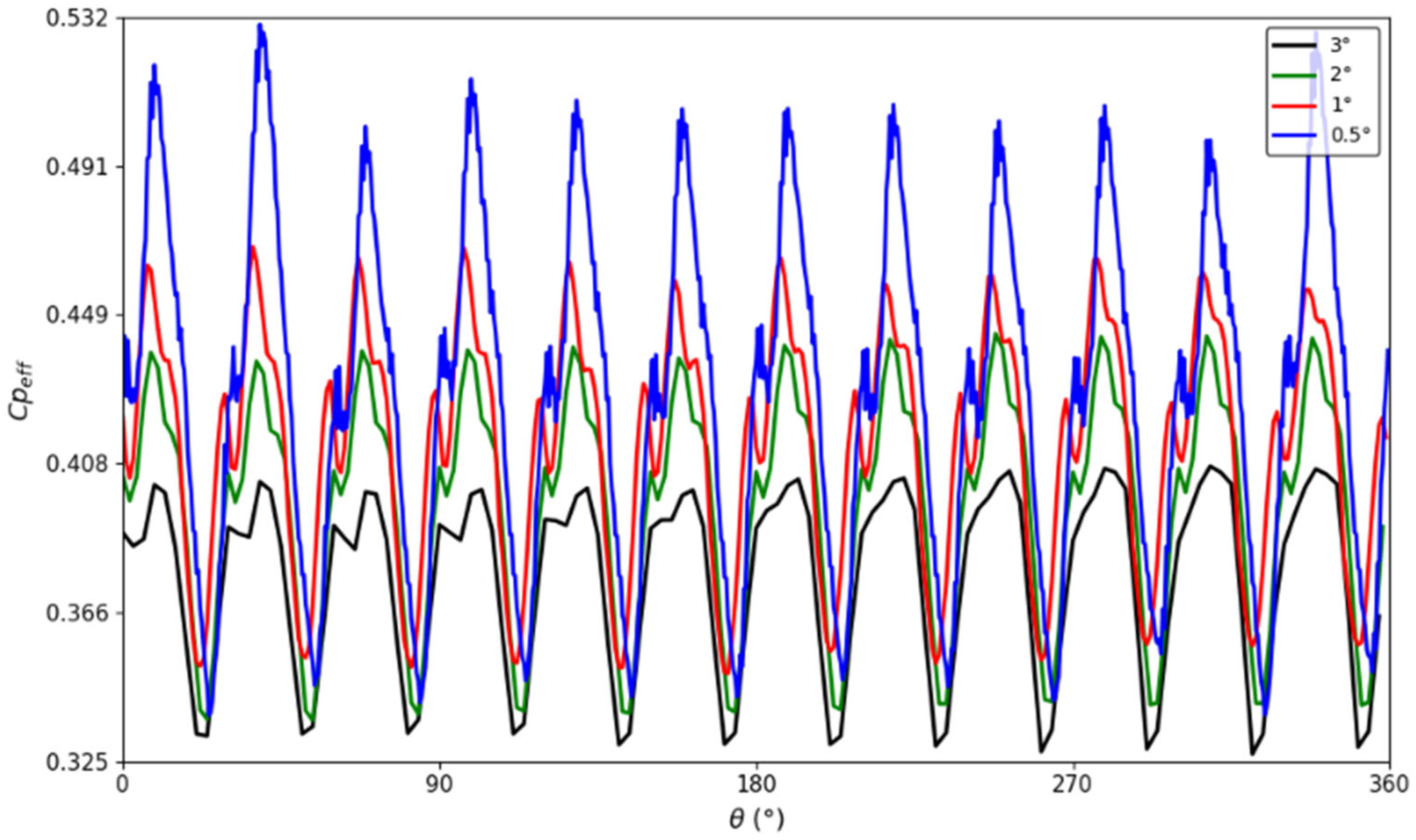
Another crucial aspect of numerical modelling verification is time step independence testing, which is carried out to identify the most suitable time step size, balancing prediction accuracy and computational cost [29]. For this purpose, four different time step sizes have been used, where each of these time step sizes corresponds to a particular angle of rotation of the wind turbine per time step. The time step sizes considered here are 3°, 2°, 1°, and 0.5° rotation of the turbine per time step. It should be noted that only statistically steady data have been used for time step size independence testing. Instantaneous Cp_eff values are plotted for one complete revolution of the wind turbine, as shown in Figure 4. Each curve in the plot shows 12 distinct peaks that correspond to the 12-bladed wind turbine model used. It can be seen that as the time step size increases, the amplitude of cyclic variations decreases. Furthermore, as the negative peaks are approximately at the same Cp_eff values in corresponding cycles, the positive peaks’ amplitude increase as the time step size decreases. This indicates that the mean Cp_eff increases as the time step size decreases.

Revolution-averaged Cp_eff values for the different time step sizes considered here are summarised in

Table 2. Variations in average power coefficient in the VAWT for different time step sizes.

Δt	Cpeff-avg	Difference
(°)	(-)	(%)
3°	0.38
2°	0.40	5.0%
1°	0.415	3.6%
0.5°	0.42	1.2%

. It is evident that Cp_eff-avg increases with a decreasing time step size. Decreasing the time step size from 3° to 2° revolution of the rotor, average Cp_eff increases from 0.38 to 0.4, i.e., 5% increase. Further decreasing the time step size to 1° increases the average Cp_eff by 3.6%, and finally, decreasing the time step size to 0.5° increases the average Cp_eff by 1.2%. Thus, a time step size of 1° has been selected for further investigations.

3. Results and Discussion

The results of this study are presented and discussed in this order: firstly, the baseline case is analysed in detail. The baseline case corresponds to a 30 mph car velocity, while the turbine is operating at a tip speed ratio (λ) of 0.3, based on the wind speed at the inlet boundary of the flow domain. Furthermore, a 30 mph car velocity represents the speed limit on the city centre roads in the UK, while λ of 0.3 is considered, as it has been reported by Gareth [21] that at this λ value, the turbine operates optimally, i.e., peak Cp. The baseline case analyses presented here include both qualitative analyses (using flow fields) and quantitative analyses (instantaneous and average power produced by the turbine). Following this, the second section discusses the effects of λ on the Cp of the turbine with a view to obtaining the full power/performance spectrum of the turbine. Lastly, the effects of car velocity on turbine power generation are presented.

3.1. Baseline Case

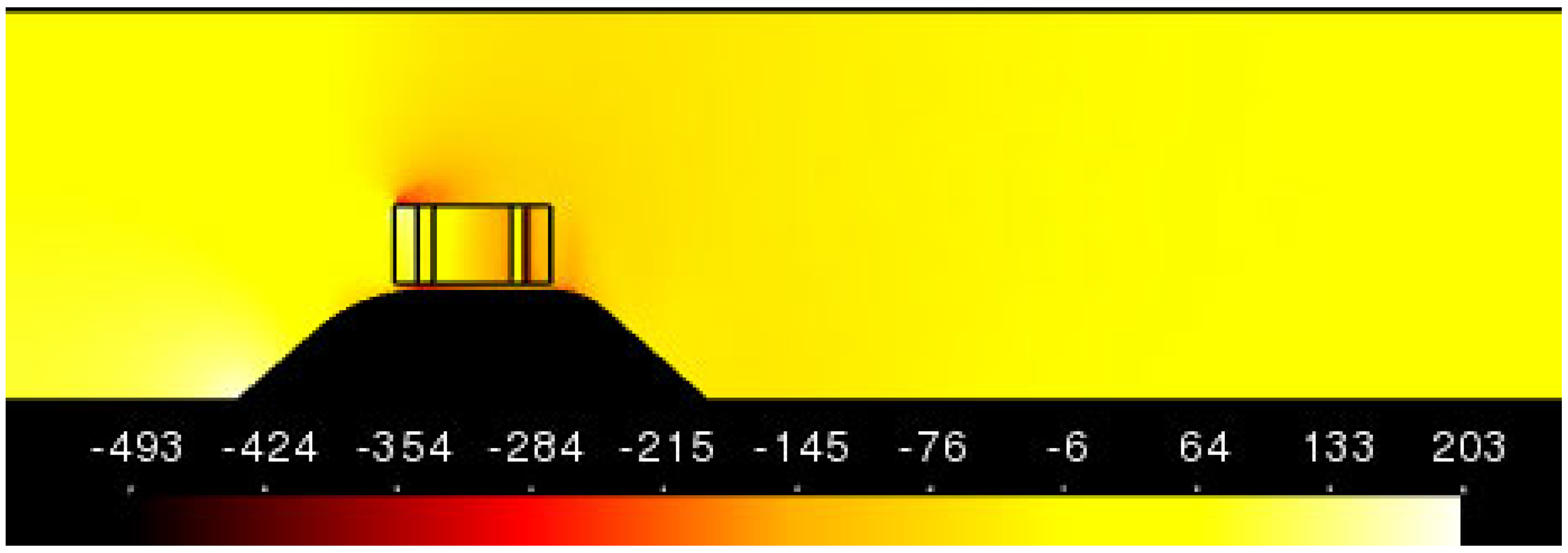
Figure 5 depicts variations in the static gauge pressure (in Pa) within the flow domain on a cross-sectional plane passing through the centre of the car and the turbine model in the Z normal direction. The static pressure variations shown range between −493 Pa,g and +203 Pa,g. It can be seen that high-pressure regions exist upstream of the car and the wind turbine, while lower pressure is observed in the immediate downstream of the turbine and above the casing. The pressure variations within the wind turbine are quite complex, with regions of high and low pressures being observed.

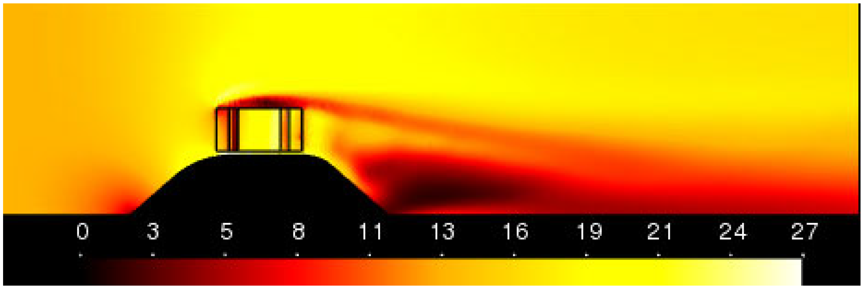
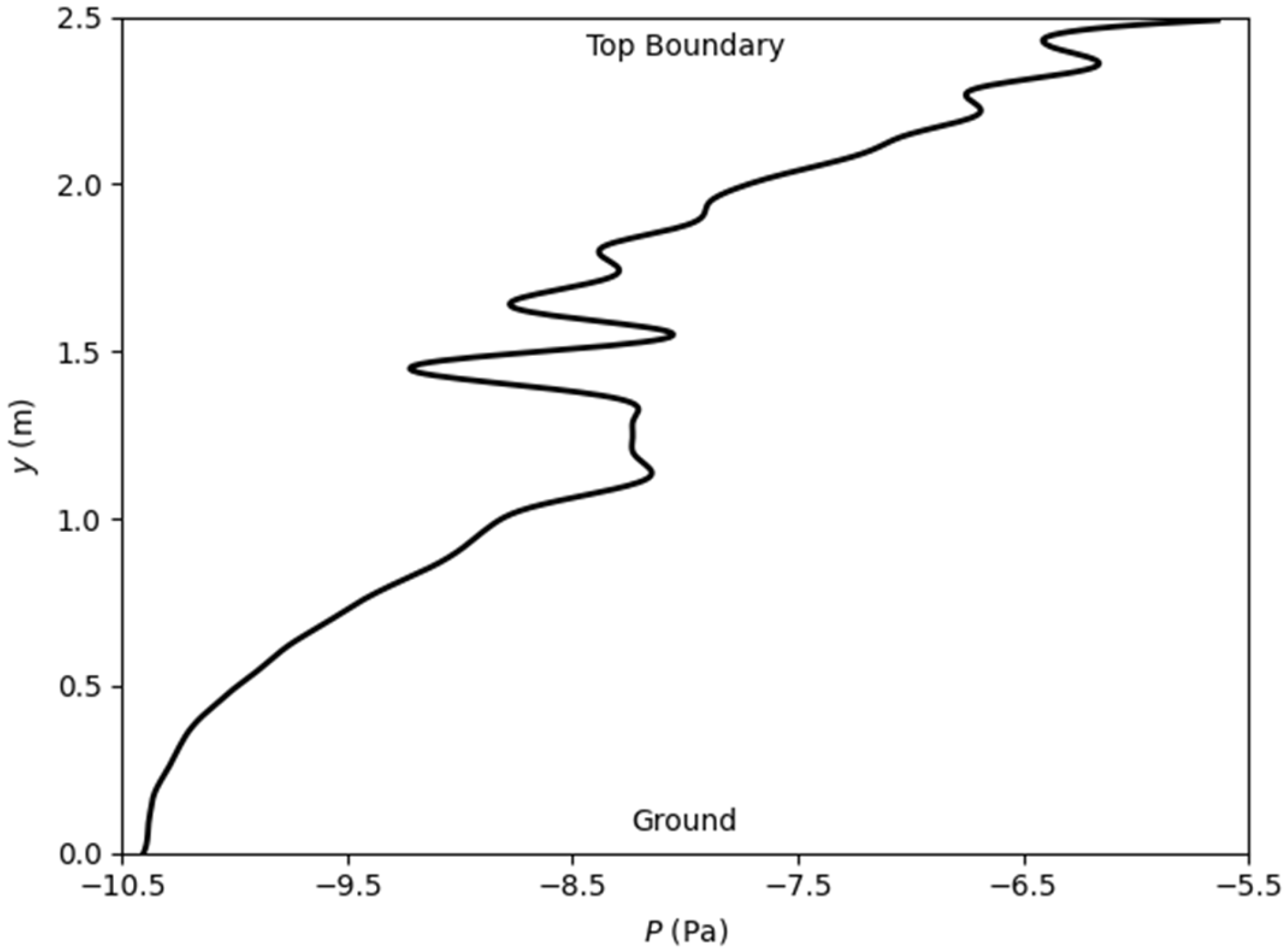
Figure 6 depicts the variations in the flow velocity magnitude (in m/s) within the flow domain. The peak flow velocity of 27 m/s is recorded within the wind turbine body on the central plane. The wake of the turbine can be clearly observed downstream of the turbine. It is being gradually deflected towards the ground due to the presence of a comparatively higher-pressure region above the wake. This is shown in Figure 7, where the pressure profile is plotted on a vertical line (y direction) downstream of the turbine at x = 4.5 m. Moreover, immediately downstream of the turbine, a high velocity region is noticed, which is a result of air flow streams exiting the turbine flow paths.

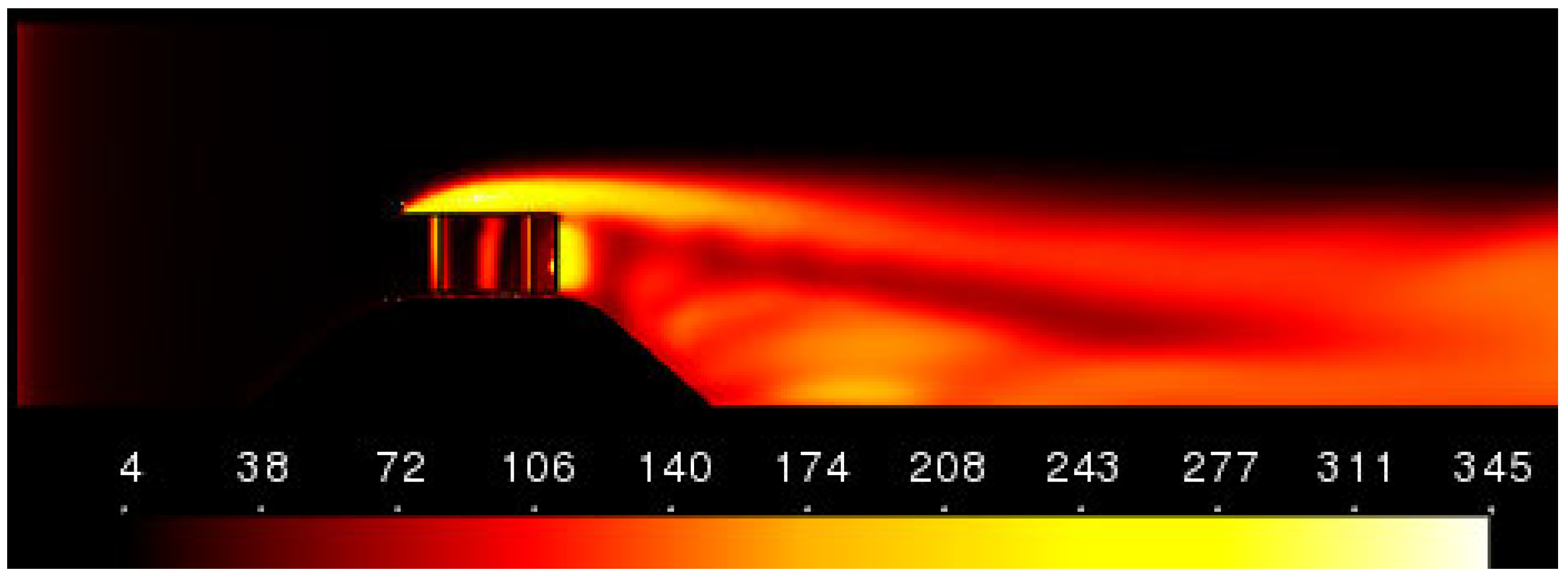
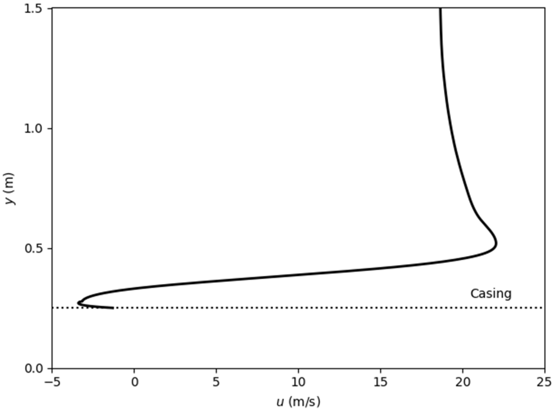
Figure 8 depicts the turbulence intensity distribution (in %) on the central plane. It can be seen that the turbulence intensity of air ranges from 4 to 345%. As expected, the wake region of the wind turbine and the car is highly turbulent [30], whereas turbulence is quite moderate in the rest of the flow domain. The highest turbulence intensity is observed at the top of the turbine casing, which is due to flow separation, leading to low velocity just above the casing, as seen in Figure 9. Further analysing the complex flow behaviour above the turbine casing, the x-direction flow velocity (u) has been plotted on a vertical line above the casing, passing through the middle of the turbine. It can be seen in Figure 9 that flow separation on the top of the casing leads to a recirculating zone, i.e., negative u velocity above the casing. The velocity gradient (du/dy) results in excessive shear, which leads to the production of turbulence, and thus, high turbulence intensity is observed above the casing.

The above analyses have helped better understand the global flow fields associated with a vertical-axis wind turbine installed on top of a car. However, local flow field analyses within the wind turbine are required for enhanced understanding and clarity [31]. For this purpose, a cross-sectional plane passing through the centre of the wind turbine in the y normal direction has been created.

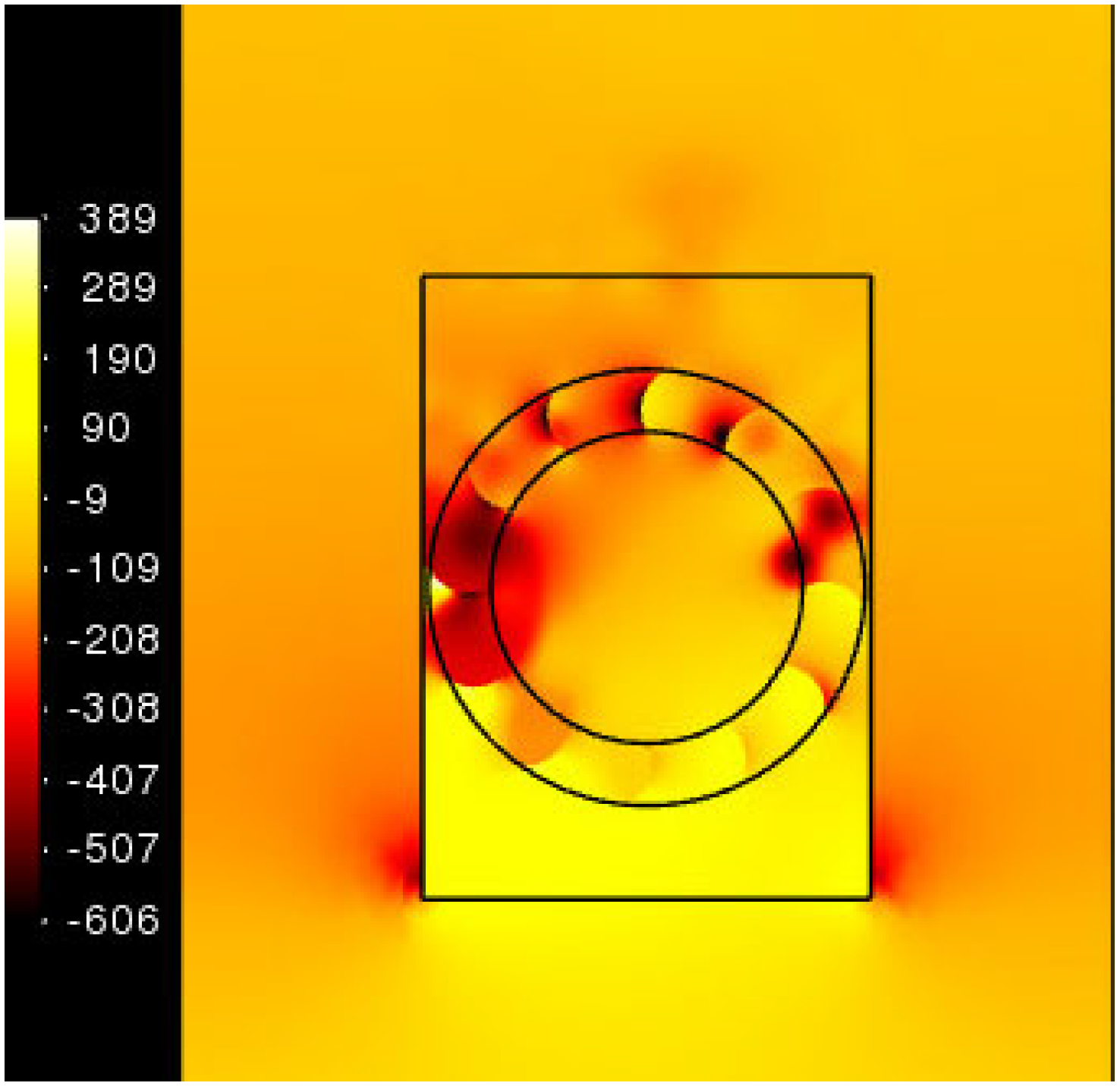
Figure 10 depicts the static gauge pressure distribution (in Pa) within the wind turbine, where the pressure ranges from −606 Pa to 389 Pa. Higher-pressure regions can be observed upstream of the wind turbine, while lower pressure regions are visible downstream of the turbine. As the flow enters the wind turbine through the flow paths between consecutive blades, depending on the orientation of the blades corresponding to the flow angle, high-pressure and low-pressure regions are created on either end of the blades, i.e., the pressure and suction sides.

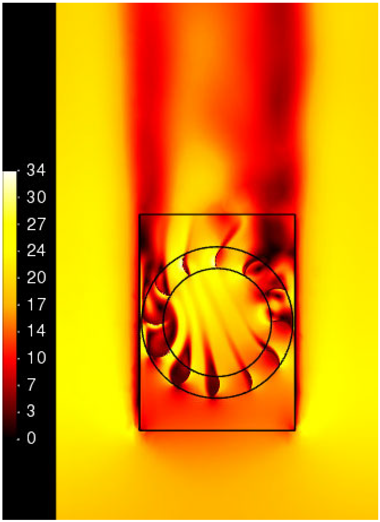
Figure 11 depicts the velocity magnitude variations (in m/s) within the wind turbine. It can be seen that air flows between the blades of the wind turbine, and depending on the orientation of the blades, the resistance offered by the blades to the air flow varies. The blades that are more in line with the incident flow offer lower resistance, and thus, their localised wake is smaller, and vice versa. The blades on either ends on the turbine (in the z direction, i.e., left and right in the figure), due to their orientation, offer excessive resistance to the flow and thus, their localised wake extends far downstream the turbine. Hence, the downstream wake of the turbine is parted with a relatively higher flow velocity region in the middle. Due to a significant velocity gradient in the downstream wake, the high velocity streak in the middle diffuses its momentum quickly and merges with the rest of the wake.

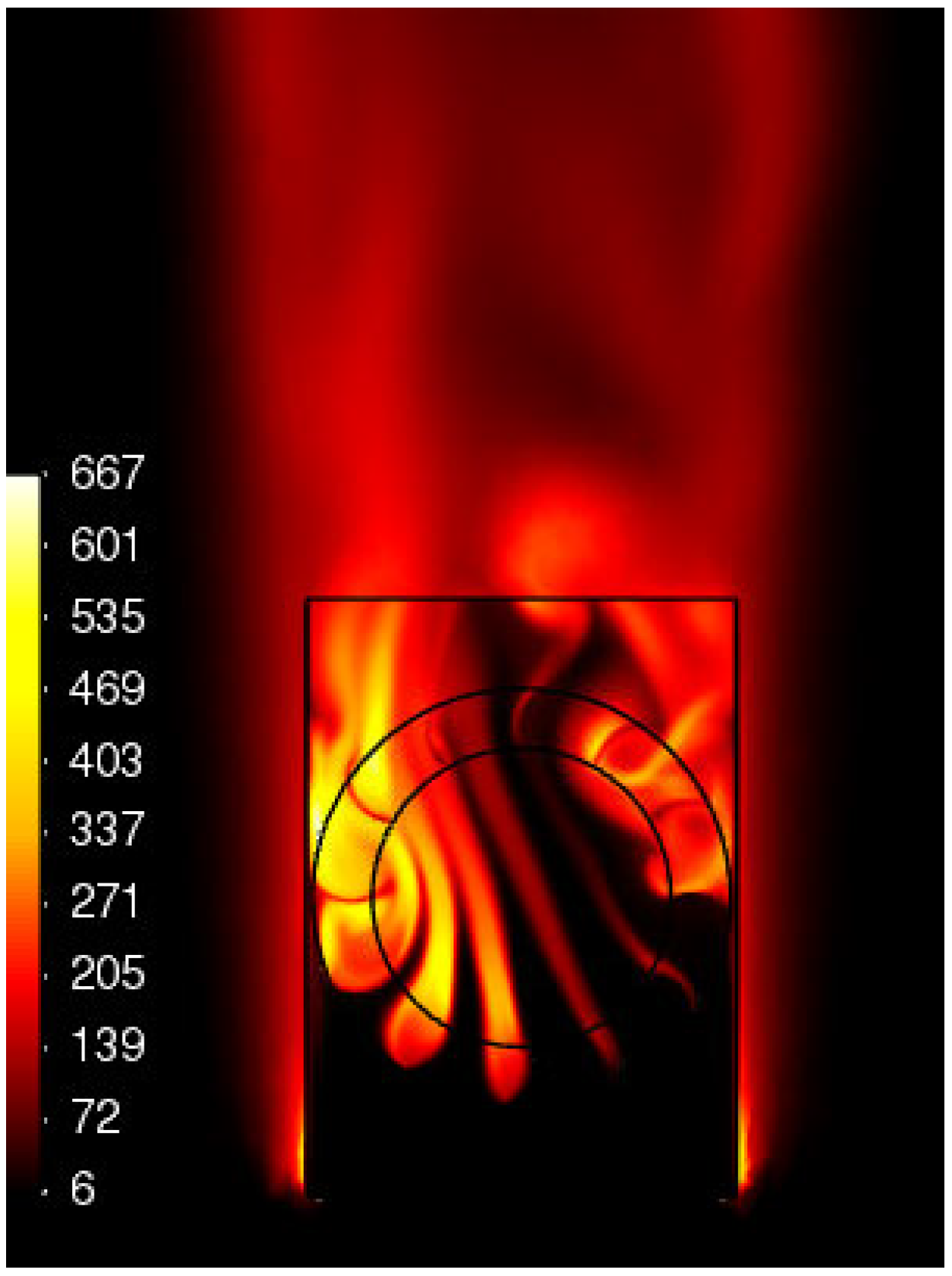
Figure 12 shows turbulence intensity variations (in %) within the wind turbine. It can be clearly seen that the turbulence is higher in both the localised wake regions of the blades and in the wake region downstream of the turbine. Hence, the turbulence intensity is higher where the flow velocity is lower (see Figure 11), and vice versa. An interesting observation is that turbulence intensity associated with the left-hand side blades (in the figure) is considerably higher than that of the blades on the right-hand side. This is due to the shape and orientation of the blades, i.e., the blades on the left-hand side are positioned such that air flow encounters convex surfaces, while on the right-hand side, it encounters concave surfaces. Air flow bifurcates on the convex surfaces, and thus, streaks of highly turbulent air can be seen propagating downstream of the blades, whereas flow impinging on concave surfaces is accumulated, resulting in comparatively lower turbulence.

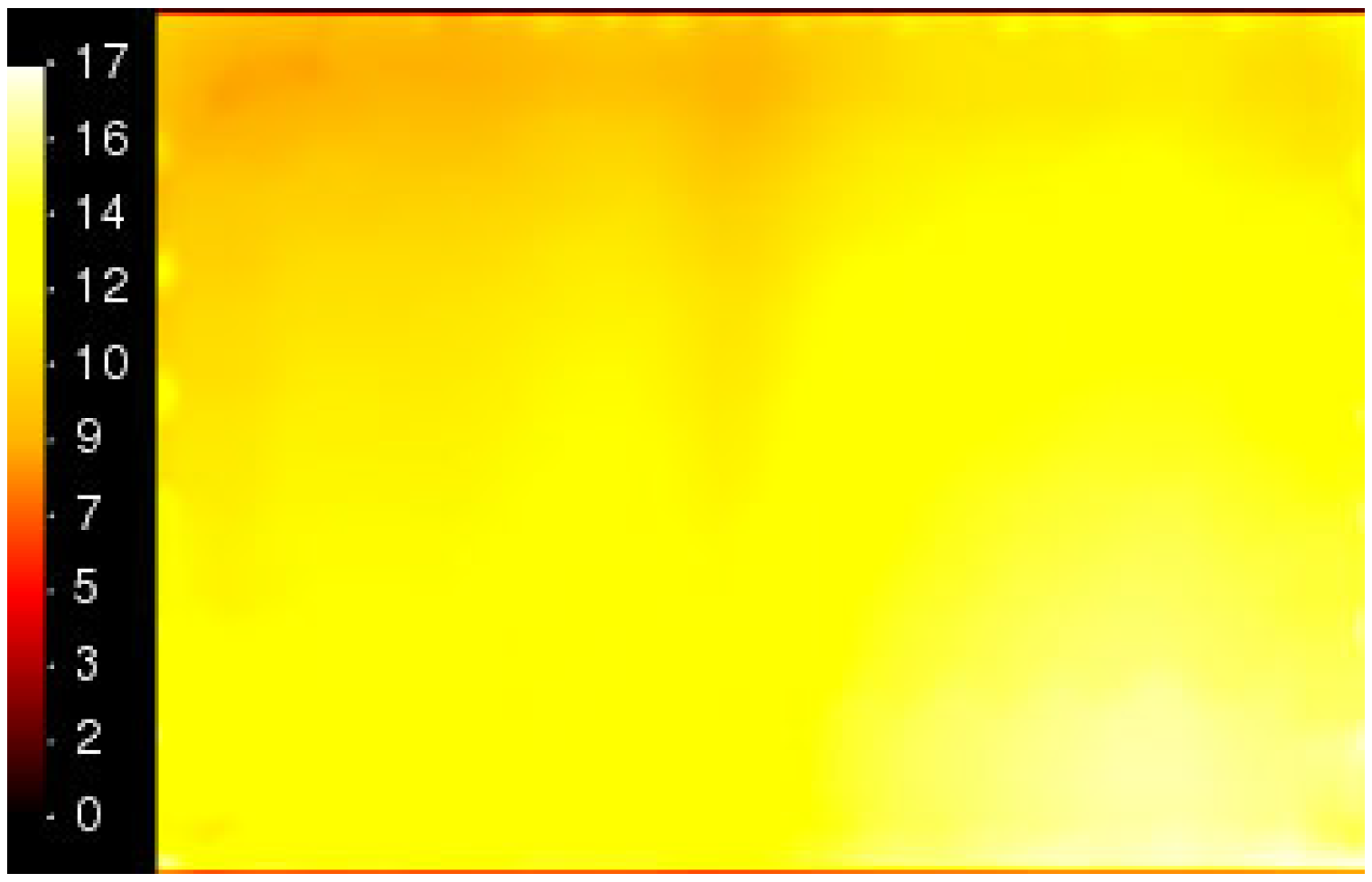
Wind turbines normally operate in theoretically free (unbounded) flow. However, in the current study, the wind turbine is housed inside a casing, and hence, the incident flow to the turbine is wall bounded. Moreover, due to the curvature of the car windscreen, the air flow entering the casing can be quite complex in nature. It is, therefore, important to analyse incident air flow conditions affecting the turbine and characterise its performance based on that. For this purpose, a cross-sectional plane inside the casing has been created upstream of the turbine, and flow velocity magnitude variations have been investigated on this plane, as shown in Figure 13. It can be seen that although the inlet velocity to the flow domain is 30 mph (or 13.41 m/s), the incident flow velocity to the turbine is much higher, reaching a maximum of 17 m/s. Moreover, the flow velocity is not uniform. In order to accommodate this in the performance evaluation of the wind turbine, average flow velocity on this plane has been calculated (U_eff) and is used to compute the effective power coefficient (Cp_eff) and effective tip speed ratio (λ_eff) of the turbine at each time step.

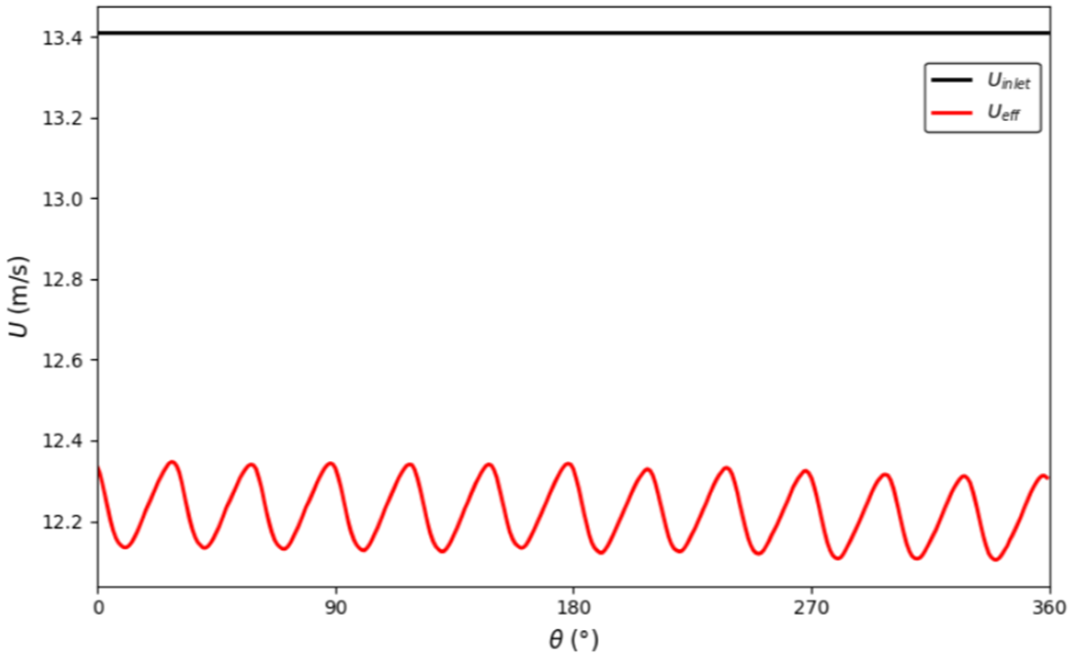
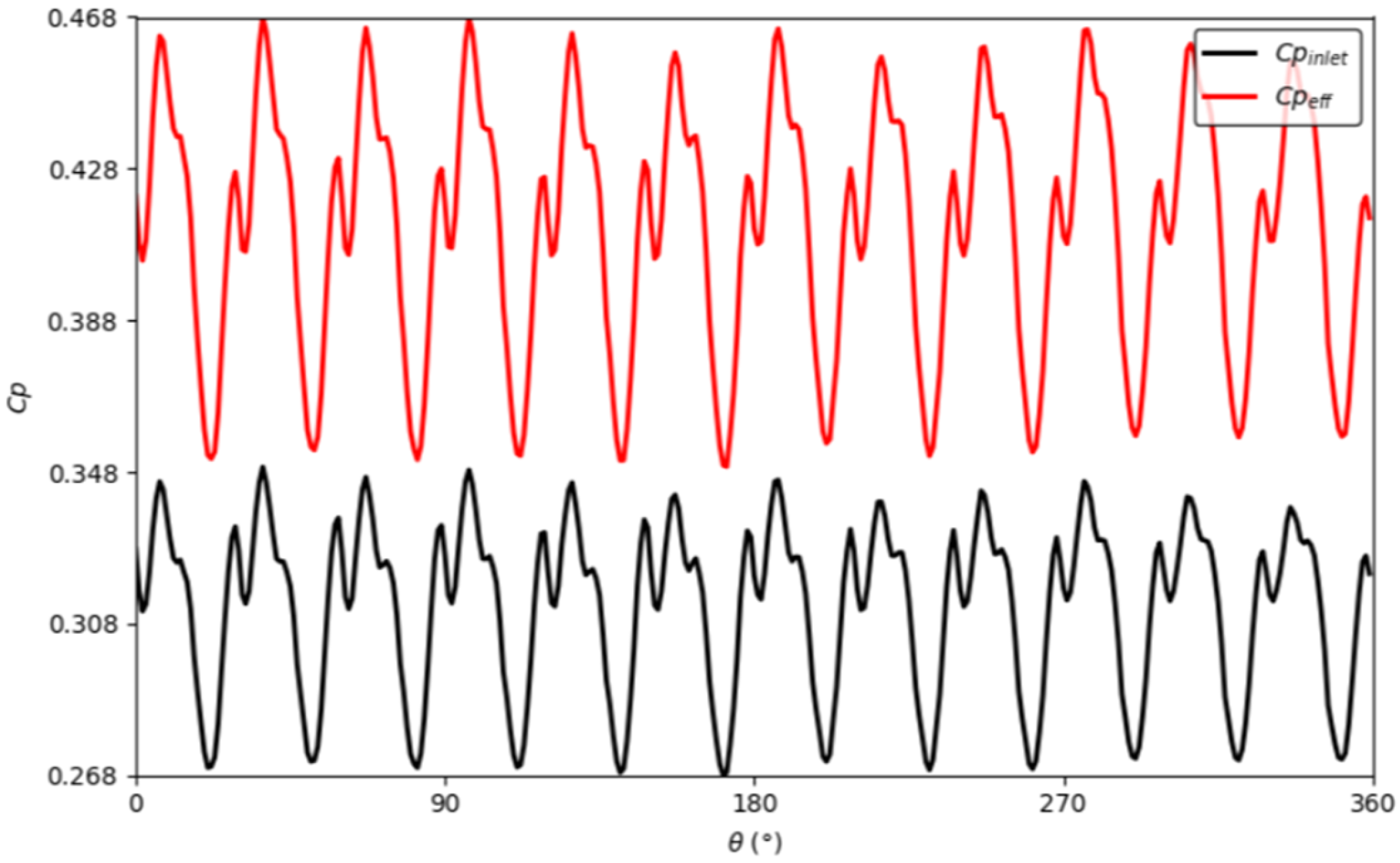
The average flow velocity incident on the wind turbine (U_eff) has been plotted and compared against the inlet (fixed) flow velocity (U_inlet) for one complete revolution of the turbine, as shown in Figure 14. It can be clearly seen that U_eff is not constant, and that it is cyclic in nature, with 12 peaks. As the turbine comprises 12 blades, the incident flow velocity is shown to be affected by the blades during the rotation of the turbine. Furthermore, a comparative analysis of Cp_inlet (based on inlet flow velocity) and Cp_eff (based on U_eff) is presented in Figure 15, where it can be clearly seen that if inlet velocity is used to calculate turbine Cp, the revolution-averaged Cp of the turbine is considerably lower (Cp_inlet-avg = 0.31) than if it is calculated using U_eff (Cp_eff-avg = 0.41). It should be noted that the Cp_eff curve in Figure 15 is the same as in Figure 4 for a 1° time step size.

3.2. Effects of Turbine’s Tip Speed Ratio (λ)

In order to capture the complete performance spectrum of the wind turbine, it must be tested at a range of tip speed ratios. It has been widely reported that the operational range of drag-based vertical-axis wind turbines is λ = 0–1 [32]. Thus, investigations have been carried out on λ values of 0.1, 0.5, 0.7, and 0.9. Note that these are λ values, based on inlet flow velocity, and not λ_eff, which is based on U_eff, as the information on U_eff is not available beforehand. Also note that the results corresponding to λ_eff = 0.33 have already been reported and discussed in the previous section.

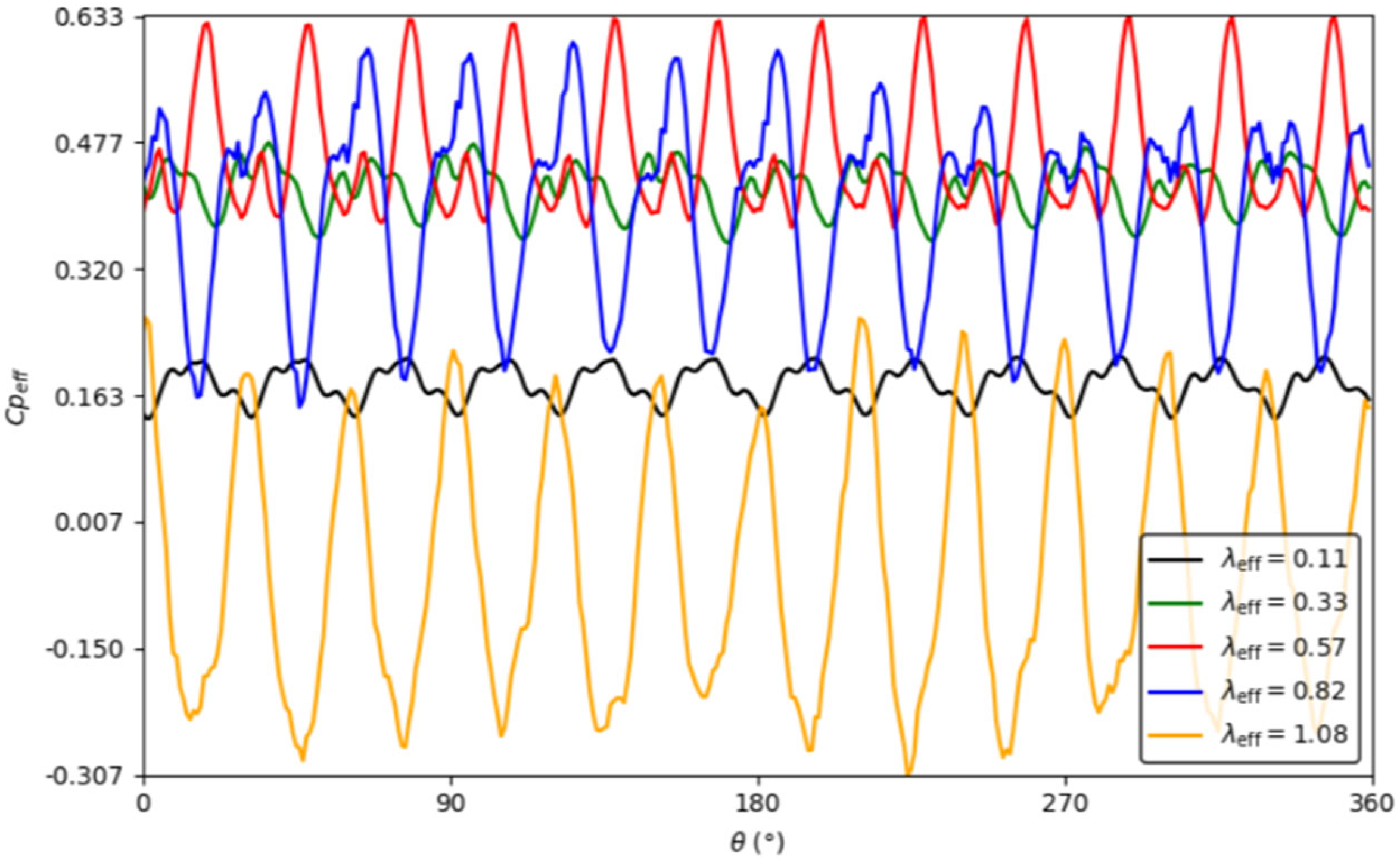
Figure 16 depicts the instantaneous variations in Cp_eff for the different λ_eff values obtained. It can be seen that the resulting λ_eff values are 0.11, 0.57, 0.82, and 1.08, respectively. Previously obtained results for λ_eff = 0.33 are also included (green curve). As observed in the case of Figure 4, all curves at different λ_eff show cyclic behaviour with 12 distinct peaks (corresponding to 12 rotor blades). There are two behaviours that can be observed. Firstly, as λ_eff increases, the amplitude of oscillations increases. As λ is a representation of the blade tip speed relative to the incident wind speed, at lower λ_eff, blades are rotating much slower compared to the wind speed, and thus, the drag force experienced by the blades stays almost constant. As the blade rotational speed increases compared to the wind speed, the drag force being exerted on the blades also increases, leading to higher amplitudes in Cp_eff.

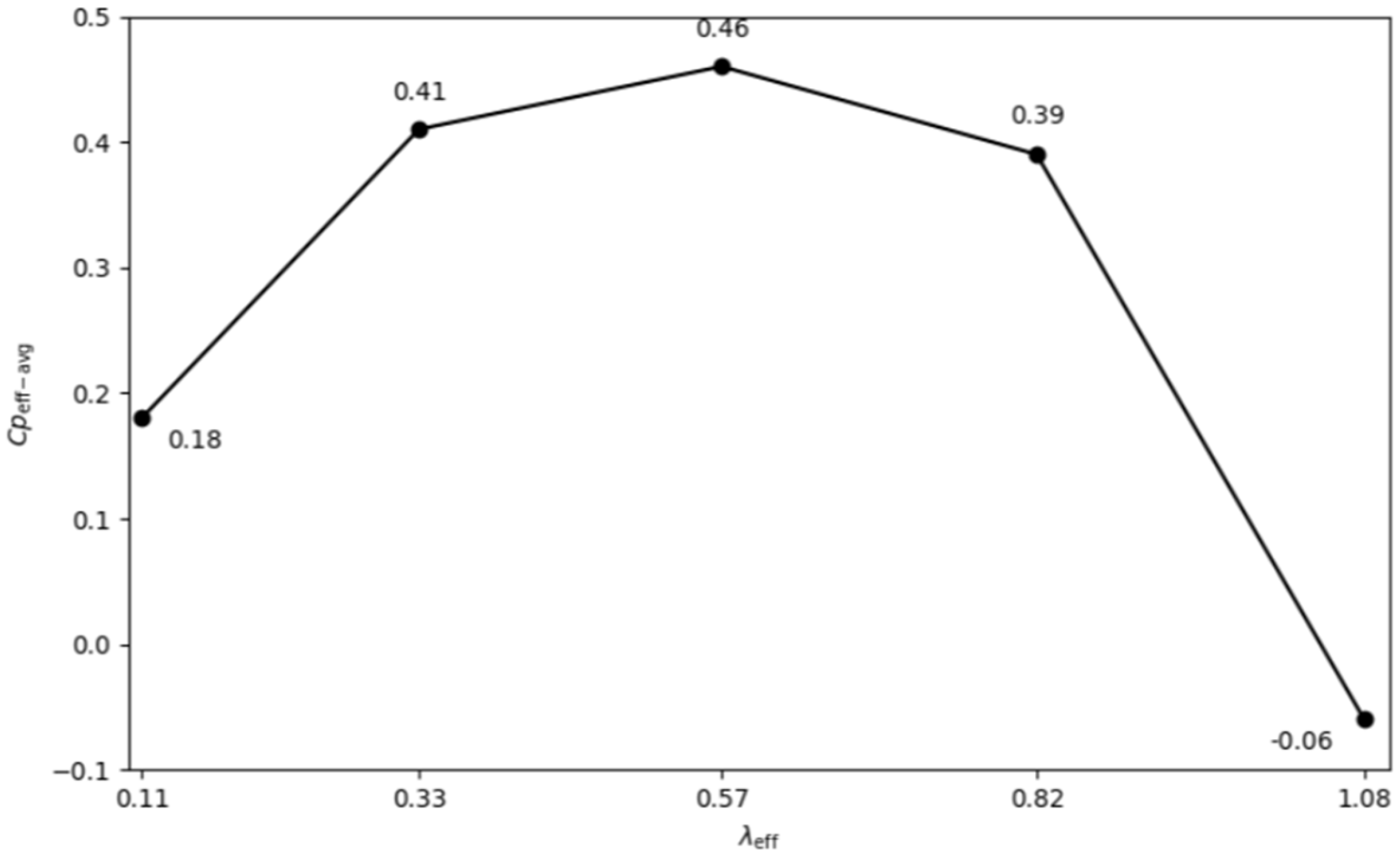
The second observation is that as the λ_eff increases until 0.57, the curves shift upwards (i.e., higher Cp_eff). A further increase in λ_eff beyond 0.57 brings the curves down (i.e., lower Cp_eff). An increase in Cp_eff as λ_eff increases is attributed to the net power produced by the turbine, i.e., power produced by the returning blades (positive power) minus the power produced by the advancing blades (negative power). As λ_eff increases to 0.57, the returning blades’ contribution to the net power of the turbine increases relative to the advancing blades’ negative power contribution. This is where the turbine produces the optimal/peak power. Further increasing the λ_eff, the advancing blades’ negative power contribution increases significantly, resulting in lower net power produced by the turbine. Eventually, at λ_eff = 1.08, the advancing blades’ negative power contribution increases beyond the returning blades’ positive power contribution, and thus, the net power produced by the turbine is negative, i.e., instead of producing power, the turbine starts to consume power in order to keep rotating at that tip speed ratio. Plotting the rotation average Cp_eff for each λ_eff in Figure 17, it can be seen that the average Cp_eff of the turbine at λ_eff = 0.11 is 0.18, which increases to 0.41 and 0.46, respectively, at λ_eff of 0.33 and 0.57. Further increasing λ_eff to 0.82 decreases the average Cp_eff to 0.39, while at λ_eff = 1.08, the average Cp_eff is −0.06.

In terms of the average power generated by the turbine (P) at different λ_eff,

Table 3. Power characteristics of the VAWT at different effective tip speed ratios.

λeff	Pmax	Pmin	Pavg
(-)	(W)	(W)	(W)
0.11	77.5	50.3	65.3
0.33	180.5	138.3	161.5
0.57	217.5	128.2	159.2
0.82	189.2	47.1	124.3
1.08	76.8	−91.2	−16.4

summarises the maximum (P_max), minimum (P_min), and average power (P_avg) values. Analysing the P_max and P_min values, it can be seen that P_max increases from 77.5 W to 217.5 W as λ_eff increases from 0.11 to 0.57. Increasing λ_eff from 0.57 to 1.08, P_max decreases to 76.8 W. Similarly, P_min increases from 50.3 W to 128.2 W, respectively, as λ_eff increases from 0.11 to 0.57, while a further increase in λ_eff to 1.08 decreases P_min to −91.2 W. Interestingly, P_avg peaks at λ_eff = 0.33 (161.5 W), while at λ_eff = 0.57, P_avg = 159.2 W. This is because of U_eff between λ_eff = 0.33 and 0.57. As Cp varies inversely with U³, while turbine power (P = ωT) varies inversely with U, a slight decrease in U_eff will have a more profound effect on Cp. In the case of λ_eff = 0.57, U_eff is 4.2% less than at λ_eff = 0.33 (11.71 m/s compared to 12.22 m/s). Thus, the power produced by the turbine at λ_eff = 0.33 is slightly higher than the power produced by the turbine at λ = 0.57, although the peak Cp_eff is observed at λ_eff = 0.57.

3.3. Effects of Car Velocity (U)

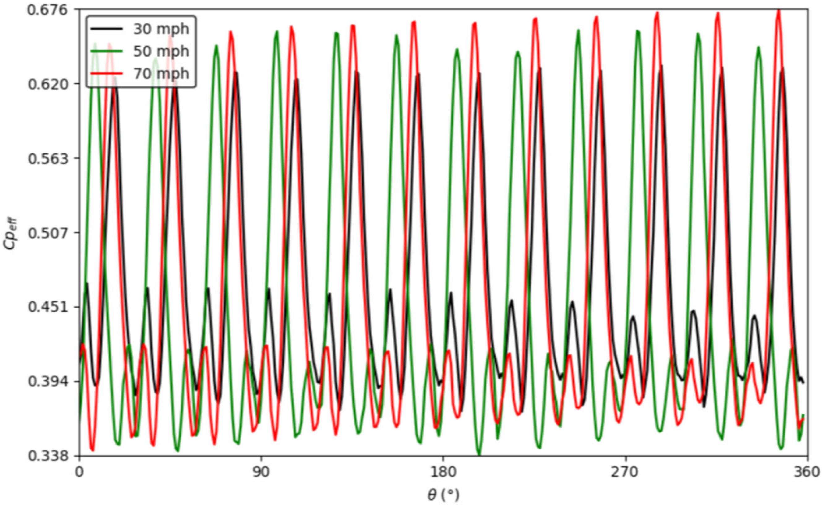
After analysing the power spectrum of the wind turbine installed on the top of the car, it becomes important to evaluate the power generated by the turbine at different car velocities. For this purpose, car velocities of 30 mph, 50 mph, and 70 mph have been selected, representing speed limits within city roads, on inter-city roads, and on motorways (in the UK). Instantaneous Cp_eff values are plotted at these car velocities in Figure 18 for one complete revolution of the turbine. For visual clarity, turbine rotation has been offset slightly so that all the curves in the figure can be easily visualised. It can be seen that at 30 mph, Cp_eff-max and Cp_eff-min are 0.63 and 0.37. Increasing the car velocity to 50 mph, Cp_eff-max increases to 0.66 while Cp_eff-min decreases to 0.34. Further increasing the car velocity to 70 mph further increases Cp_eff-max to 0.68 while keeping Cp_eff-min the same, i.e., 0.34.

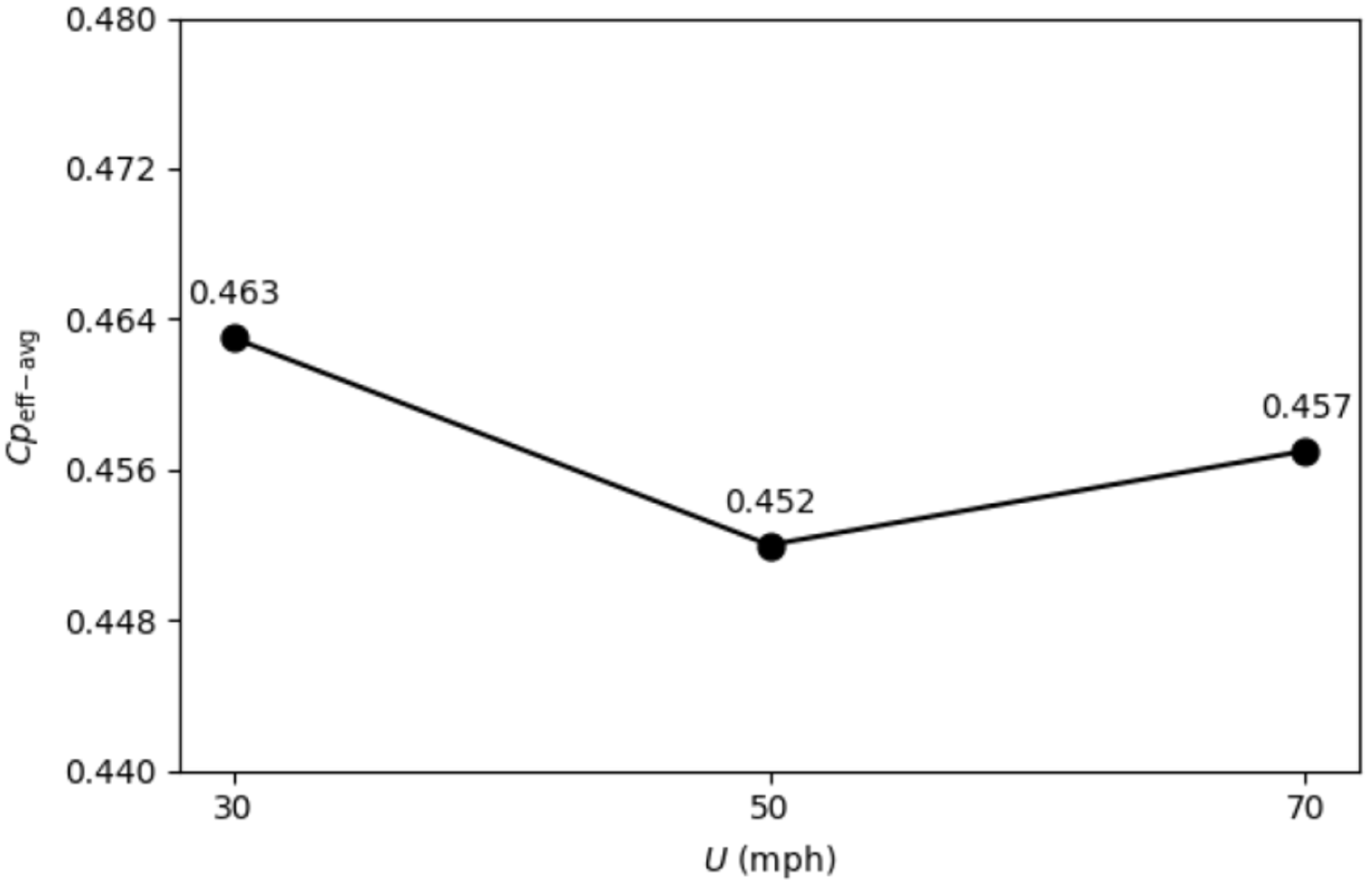
The net result of these variations is plotted in terms of revolution-averaged Cp_eff at different car velocities, as shown in Figure 19. It can be seen that there is a very small difference in Cp_eff between the car velocities considered here. At 30 mph, the average Cp_eff is 0.463, while at 50 mph and 70 mph, the values are 0.452 and 0.457, respectively. The difference between maximum Cp_eff-avg (at 30 mph) and minimum Cp_eff-avg (at 50 mph) is merely 2.3%. Thus, it can be concluded that the car velocity has a minimal effect on the Cp_eff of the turbine. However, the actual power generated by the turbine will be significantly different as the car velocities are considerably different.

Table 4. Power characteristics of the VAWT at different inlet velocities.

U	Pmax	Pmin	Pavg
(mph)	(W)	(W)	(W)
30	217.5	128.2	159.2
50	1022.1	524.1	702.2
70	2882	1387.8	1954.7

summarises the P_max, P_min, and P_avg values at different car velocities, based on the results shown in Figure 18. It can be clearly seen that the average power produced by the turbine at 30 mph, 50 mph, and 70 mph is 159 W, 702 W, and 1955 W, respectively. Thus, at a cruising speed on motorways, the turbine installed on the top of the car will produce approximately 2 kW of power, which can be used to recharge the batteries of the electric vehicle.

3.4. Net Energy Balance

The net energy balance of the car and VAWT assembly has been carried out to identify potential energy deficits and areas of improvement. For this purpose, the drag characteristics of the car alone at different wind speeds have been obtained. As only the top half of the car is considered in this study, total drag on the car is computed based on a conservative estimate of 35% drag contribution from the wind screen, roof, and the rear screen in a typical car [33]. Following this, the total drag on the assembly of the car and VAWT is calculated, which highlights the drag contribution of the VAWT alone. Finally, the contribution of VAWT’s drag to the total drag has been computed. The results are summarised in

Table 5. Drag characteristics of the car and VAWT at different inlet velocities.

U	Dcar-top	Dcar-total	DVAWT	DTotal	$\frac{{\mathit{D}}_{\mathit{V}\mathit{A}\mathit{W}\mathit{T}}}{{\mathit{D}}_{\mathit{T}\mathit{o}\mathit{t}\mathit{a}\mathit{l}}}$
(mph)	(N)	(N)	(N)	(N)	(%)
30	120	343	70	413	17
50	330	943	193	1136	17
70	643	1837	382	2219	17

. It can be seen that at different wind speeds considered in this study, the drag contribution from the VAWT is consistently 17%, i.e., 17% of additional drag is experienced by the car when the VAWT is installed on its roof.

In order to quantify the overall energy balance of the VAWT–car assembly, the additional power required to overcome aerodynamic drag from the VAWT has been calculated as:

$$P_{drag}=D_{VAWT}\times U$$

(5)

where P_drag is the additional power required to overcome aerodynamic drag due to the VAWT (D_VAWT).

Table 6. Net energy balance of the VAWT–car assembly.

U	DVAWT	Pdrag	Pavg	Net Energy Balance
(mph)	(N)	(W)	(W)	(W)
30	70	939	159	−780
50	193	4314	702	−3612
70	382	11,953	1954	−9998

summarises the additional power in comparison with the electrical power generated by the VAWT.

The results clearly indicate that the additional power required to overcome aerodynamic drag due to the VAWT is substantially higher than the electric power generated by it. Thus, the present configuration results in a net negative energy balance at all vehicle speeds considered. However, it is important to note that the primary objective of the current study is not to demonstrate an immediately deployable EV charging system, but rather to investigate the aerodynamic and power generation characteristics of a high-output drag-based VAWT operating under varying flow conditions. The results obtained show that the proposed system produces considerably higher power compared to previously reported vehicle-integrated VAWTs, thereby providing a basis for future optimisation studies aimed at reducing aerodynamic drag penalties and improving the overall system’s energy balance.

It should be noted that a full-vehicle aerodynamic drag coefficient analysis was beyond the scope of the present study, and only the upper vehicle geometry was modelled in order to reduce computational costs. Nevertheless, direct CFD-based drag force calculations provide a sufficiently robust basis for comparative assessment of the aerodynamic impact of the VAWT configuration investigated.

4. Conclusions

Numerical investigations on the performance characteristics of an innovative drag-based vertical-axis wind turbine installed on the top of an electric vehicle have been carried out in this study with the aim of investigating the aerodynamic behaviour and power generation characteristics of a drag-based VAWT operating at various vehicle speeds. Computational fluid dynamics-based transient solvers have been employed for the transient flow of air across the top half of the vehicle and the boxed design of a 12-bladed turbine. Investigations have been carried out at vehicle speeds of 30 mph, 50 mph, and 70 mph, representing city centre, inter-city, and motorway speed limits, respectively. For complete performance characterisation of the turbine, investigations have been carried out at tip speed ratios of 0.1, 0.3, 0.5, 0.7, and 0.9. Flow field analyses have been carried out in detail utilising pressure, velocity, and turbulence variations, while both instantaneous and revolution-averaged power output of the turbine have been plotted.

The results obtained in the current study show the complex aerodynamics associated with the wind turbine mounted on the top of a car, as both their wakes interact with each other. Turbine’s wake is deflected downwards due to ground effects. The flow velocity incident on the turbine has been found to be lower than the freestream air velocity due to the boxed design and air flow following the incline of the windscreen. Effective flow velocities, tip speed ratios, and power coefficients have thus been calculated, resulting in a 10% increase in the power coefficient of the turbine. Contrary to previous studies on this wind turbine that show peak Cp at λ = 0.3, due to U_eff, the peak Cp of 0.46 is recorded at λ_eff = 0.57, at which the average power produced by the turbine is 160 W, at a car velocity of 30 mph. This is significantly higher than the previously reported power produced by wind turbines installed on EVs. Increasing the car velocity does not result in any noticeable increase or decrease in the Cp_eff of the turbine. At 70 mph, the average power produced by the turbine is about 2 kW. A net energy deficit is recorded at all wind speeds due to the additional drag from the turbine. Overall, the present study demonstrates the aerodynamic feasibility and comparatively high-power generation capability of the proposed configuration under different vehicle speeds. Although the current configuration results in a net negative energy balance due to additional aerodynamic drag, the findings establish a basis for future optimisation studies focusing on turbine placement, casing aerodynamics and drag reduction, along with experimental road testing.

References

1. Steinsträter, M.; Heinrich, T.; Lienkamp, M. Effect of Low Temperature on Electric Vehicle Range. World Electr. Veh. J. 2021, 12, 115. [Google Scholar] [CrossRef]
2. He, X.; Hu, Y. Optimal Mileage of Electric Vehicles Considering Range Anxiety and Charging Times. World Electr. Veh. J. 2023, 14, 21. [Google Scholar] [CrossRef]
3. Chakraborty, P.; Parker, R.; Hoque, T.; Cruz, J.; Du, L.; Wang, S.; Bhunia, S. Addressing the range anxiety of battery electric vehicles with charging en route. Sci. Rep. 2022, 12, 5588. [Google Scholar] [CrossRef] [PubMed]
4. Lanz, L.; Noll, B.; Schmidt, T.S.; Steffen, B. Comparing the levelized cost of electric vehicle charging options in Europe. Nat. Commun. 2022, 13, 5277. [Google Scholar] [CrossRef] [PubMed]
5. Azzouz, L.; Brand, C.; Fawcett, T.; Zhou, Z.; Altaf, M. Beyond the plug: Enhancing the user experience at public electric vehicle (EV) charging hubs. Insights from a multi-site UK study. J. Transp. Geogr. 2026, 131, 104530. [Google Scholar] [CrossRef]
6. Ferdous, S.M.; Bin Khaled, W.; Ahmed, B.; Salehin, S. Electric Vehicle with Charging Facility in Motion using Wind Energy. In Proceedings of the World Renewable Energy Congress 2011, Linköping, Sweden, 8–11 May 2011; Sustainable Transport (ST): Singapore, 2011. [Google Scholar]
7. Awal, M.R.; Jusoh, M.; Sakib, M.N.; Hossain, F.S.; Che Beson, M.R.; Aljunid, S.A. Design and implementation of vehicle mounted wind turbine. ARPN J. Eng. Appl. Sci. 2015, 10, 8699–8706. [Google Scholar]
8. Fathabadi, H. Possibility of utilizing wind turbine to recover a portion of the kinetic energy losses of a car. IEEE Trans. Veh. Technol. 2019, 68, 8663–8670. [Google Scholar] [CrossRef]
9. Goushcha, O.; Felicissimo, R.; Danesh-Yazdi, A.H.; Andreopoulos, Y. Exploring harnessing wind power in moving reference frames with application to vehicles. Adv. Mech. Eng. 2019, 11, 1687814019865689. [Google Scholar] [CrossRef]
10. Khan, Z.A.; Sherazi, H.H.R.; Ali, M.; Imran, M.A.; Rehman, I.U.; Chakrabarti, P. Designing a Wind Energy Harvester for Connected Vehicles in Green Cities. Energies 2021, 14, 5408. [Google Scholar] [CrossRef]
11. El, E.; Yildiz, C.; Dandil, B.; Yildiz, A. Effect of wind turbine designed for electric vehicles on aerodynamics and energy performance of the vehicle. Therm. Sci. 2022, 26, 2907–2917. [Google Scholar] [CrossRef]
12. Mekapati, S.R.; Choudhury, N.B.D. Power generation in electric vehicle through wind turbine. In Proceedings of the 2024 IEEE 1st International Conference on Green Industrial Electronics and Sustainable Technologies (GIEST), Imphal, India, 25–26 October 2024; pp. 1–7. [Google Scholar]
13. Mekapati, S.R.; Choudhury, N.B.D. Impact of power generation in wind turbine integrated electric vehicles over different purposes: A case study. Arab. J. Sci. Eng. 2025, 51, 8119–8148. [Google Scholar] [CrossRef]
14. Zhao, Z.; Li, Y.; Zhang, B.; Wang, C.; Yan, Z.; Wang, Q. Design and Analysis of a Novel Adjustable SVAWT for Wind Energy Harvesting in New Energy Vehicle. World Electr. Veh. J. 2022, 13, 242. [Google Scholar] [CrossRef]
15. Almahmoud, O.; Karakaya, A. Analysis of the Effect of Wind Turbines Used in Electric Vehicles on Drag Power. Teh. Vjesn. 2026, 33, 593–602. [Google Scholar]
16. Roy, S.; Saha, U.K. Review on the Numerical Investigations into the Design and Development of Savonius Wind Rotors. Renew. Sustain. Energy Rev. 2013, 24, 73–83. [Google Scholar] [CrossRef]
17. Asim, T. Computational Fluid Dynamics based Diagnostics and Optimal Design of Hydraulic Capsule Pipelines. Ph.D. Thesis, University of Huddersfield, Huddersfield, UK, 2013. [Google Scholar]
18. Versteeg, H.K.; Malalasekera, W. An Introduction to Computational Fluid Dynamics: The Finite Volume Method, 2nd ed.; Pearson Education Limited: Harlow, UK, 2007. [Google Scholar]
19. Craig, M.; Asim, T. Numerical Investigations on the Propagation of Fire in a Railway Carriage. Energies 2020, 13, 4999. [Google Scholar] [CrossRef]
20. Anderson, J.D. Computational Fluid Dynamics: The Basics with Applications; McGraw-Hill: New York, NY, USA, 1995. [Google Scholar]
21. Gareth, C. Design, Operation and Diagnostics of a Vertical Axis Wind Turbine. Ph.D. Thesis, University of Huddersfield, Huddersfield, UK, 2012. [Google Scholar]
22. Durkacz, J.; Islam, S.; Chan, R.; Fong, E.; Gillies, H.; Karnik, A.; Mullan, T. CFD modelling and prototype testing of a vertical axis wind turbines in planetary cluster formation. Energy Rep. 2021, 7, 119–126. [Google Scholar] [CrossRef]
23. Ferziger, J.H.; Perić, M. Computational Methods for Fluid Dynamics, 3rd ed.; Springer: Berlin/Heidelberg, Germany, 2002. [Google Scholar]
24. Elkhoury, M.; Kiwata, T.; Aoun, E. Experimental and numerical investigation of a three-dimensional vertical-axis wind turbine with variable-pitch. J. Wind Eng. Ind. Aerodyn. 2015, 139, 111–123. [Google Scholar] [CrossRef]
25. Menter, F.L. Zonal Two Equation k-ω Turbulence Models for Aerodynamic Flows. In Proceedings of the 23rd Fluid Dynamics, Plasmadynamics, and Lasers Conference, Orlando, FL, USA, 6–9 July 1993; p. 2906. [Google Scholar]
26. ANSYS, Inc. ANSYS Fluent User’s Guide, Release 2021 R2; ANSYS, Inc.: Canonsburg, PA, USA, 2021. [Google Scholar]
27. Abd Halim, M.A.; Nik Mohd, N.A.R.; Mohd Nasir, M.N.; Dahalan, M.N. The evaluation of k-ε and k-ω turbulence models in modelling flows and performance of S-shaped diffuser. Int. J. Automot. Mech. Eng. 2018, 15, 5161–5177. [Google Scholar] [CrossRef]
28. Almohammadi, K.M.; Ingham, D.B.; Ma, L.; Pourkashan, M. Computational fluid dynamics (CFD) mesh independency techniques for a straight blade vertical axis wind turbine. Energy 2013, 58, 483–493. [Google Scholar] [CrossRef]
29. Leishman, J.G. Challenges in modelling the unsteady aerodynamics of wind turbines. Wind Energy 2002, 5, 85–132. [Google Scholar] [CrossRef]
30. Ahmed, S.R.; Ramm, G.; Faltin, G. Some salient features of the time-averaged ground vehicle wake. In Proceedings of the SAE International Congress and Exposition, Detroit, MI, USA, 27 February 1984; SAE Technical Paper 840300; SAE: Warrendale, PA, USA, 1984. [Google Scholar]
31. Liu, X.; Zhu, G.; Asim, T.; Zhang, Y.; Mishra, R. The Innovative Design of Air Caps for Improving the Thermal Efficiency of CFB Boilers. Energy 2021, 221, 119844. [Google Scholar] [CrossRef]
32. Manwell, J.F.; McGowan, J.G.; Rogers, A.L. Wind Energy Explained: Theory, Design and Application, 2nd ed.; John Wiley & Sons Ltd.: Chichester, UK, 2009. [Google Scholar]
33. Hucho, W.-H. (Ed.) Aerodynamics of Road Vehicles: From Fluid Mechanics to Vehicle Engineering; Butterworth-Heinemann: Oxford, UK, 1987. [Google Scholar]
Figure 1. Geometrical modelling of the VAWT mounted on an EV (a) dimensions and CAD model of the VAWT (b) dimensions of the flow domain.
Sustainability 18 05079 g001
Figure 2. Meshing inside the flow domain and the VAWT.
Sustainability 18 05079 g002
Figure 3. Mesh independence testing results.
Sustainability 18 05079 g003
Figure 4. Time step independence testing results.
Sustainability 18 05079 g004
Figure 5. Static pressure variations on the centre plane.
Sustainability 18 05079 g005
Figure 6. Flow velocity variations on the centre plane.
Sustainability 18 05079 g006
Figure 7. Static pressure profile on a vertical line downstream of the VAWT.
Sustainability 18 05079 g007
Figure 8. Turbulence intensity variations on the centre plane.
Sustainability 18 05079 g008
Figure 9. Velocity magnitude profile on a vertical line passing through the centre of the VAWT.
Sustainability 18 05079 g009
Figure 10. Static pressure variations in the vicinity of the VAWT.
Sustainability 18 05079 g010
Figure 11. Velocity magnitude variations in the vicinity of the VAWT.
Sustainability 18 05079 g011
Figure 12. Turbulence intensity variations in the vicinity of the VAWT.
Sustainability 18 05079 g012
Figure 13. Flow velocity variations in the casing upstream of the VAWT.
Sustainability 18 05079 g013
Figure 14. Comparison of inlet velocity and the effective flow velocity inside the casing upstream of the VAWT.
Sustainability 18 05079 g014
Figure 15. Instantaneous power coefficient of the VAWT based on inlet and effective velocities.
Sustainability 18 05079 g015
Figure 16. Instantaneous effective power coefficient of the VAWT at different effective tip speed ratios.
Sustainability 18 05079 g016
Figure 17. Revolution-averaged effective power coefficient of the VAWT at different effective tip speed ratios.
Sustainability 18 05079 g017
Figure 18. Instantaneous effective power coefficient of the VAWT at different inlet velocities.
Sustainability 18 05079 g018
Figure 19. Revolution-averaged effective power coefficient of the VAWT at different inlet velocities.
Sustainability 18 05079 g019