Machine Learning-Based Forecasting of Waste Generation Proxies Under Data-Limited Conditions for Supporting Adaptive and Sustainable Citarum River Management

Abstract

This study addresses the prediction of daily waste generation dynamics under data-limited conditions in a strategic watershed serving over 25 million residents. A machine learning framework is developed using daily proxies reconstructed from annual data (2019–2024) through an additive seasonal stochastic disaggregation approach, while maintaining consistency with official SIPSN records. Statistical analysis identifies the 2023 annual total as anomalous (+127.06% YoY) using the IQR method, while sensitivity tests to various parameter configurations indicate that the baseline setting (α = 0.95; σ_frac = 0.08) provides stable estimates. Four models—Random Forest, Support Vector Regression (SVR), XGBoost, and Long Short-Term Memory (LSTM)—are evaluated using strict chronological partitioning to maintain temporal integrity. Results indicate that the evaluation reflects the model’s ability to reproduce synthetic proxies, rather than direct field observations. SVR performed best (R² = 0.8157; RMSE = 881.43 t/day), outperforming the persistence baseline by +32.2%. After data leakage correction, XGBoost’s performance decreased significantly (R² = 0.1591). Feature analysis confirmed the dominance of short-term statistical indicators, while the hierarchical bootstrap approach produced more comprehensive uncertainty estimates, with SVR remaining the most stable across seasons.

1. Introduction

The Citarum River is the longest river in West Java, Indonesia, extending approximately 297 km from its headwaters in Mount Wayang to its outlet in the Java Sea [1]. Draining a catchment area of about 6614 square kilometers, it functions as a critical water resource system supporting domestic supply, agricultural irrigation, hydropower generation, and industrial activities for millions of residents. More than 25 million people depend on this river basin, particularly in Bandung City and the surrounding urbanized regions. Despite its strategic importance, the river has suffered severe environmental degradation driven by persistent anthropogenic pressures and inadequate waste management.

Among these, solid waste pollution represents one of the most dominant environmental challenges affecting the Citarum River and its ecological sustainability. Domestic waste contributes approximately 83.5% of total pollution loads, reaching up to 158,016 kg per day [2,3]. Industrial activities, particularly textile manufacturing, further intensify contamination through chemical discharges, including high concentrations of biochemical oxygen demand and chemical oxygen demand [2,3]. In addition, microplastic contamination has been reported, with concentrations reaching 3.35 particles per cubic meter in river water [2,3].

These pollution sources have led to significant accumulation of waste within the river system, particularly in downstream urban segments. Field observations by Cordova et al. [4] reveal substantial accumulation of macroplastics and microplastics in densely populated areas. Macroplastic concentrations have reached 2.91 ± 1.116 items per cubic meter, with daily debris discharge exceeding one ton [4]. Zainalarifin et al. [5] further report that such conditions significantly degrade water quality and disrupt aquatic ecosystems. As a consequence, these impacts increase flood risks and hinder progress toward Sustainable Development Goals (SDGs) related to clean water and sustainable urban environments [5].

Beyond the magnitude of pollution, the dynamics of riverine waste are inherently complex and shaped by multiple interacting processes. Riverine waste behavior is governed by the interplay between waste generation, hydrological processes, and human activities across spatial and temporal scales. Van Emmerik et al. [6] demonstrate that waste transport is strongly influenced by hydrological conditions, particularly during high-flow events. Hurley et al. [7] show that lightweight plastics are more easily mobilized during floods, while heavier materials tend to accumulate and remobilize episodically. Furthermore, Van Emmerik and Schwarz [8] highlight that extreme events disproportionately control annual plastic transport, underscoring the nonlinear, event-driven nature of riverine waste systems.

Despite this understanding, accurately quantifying these dynamics remains a major challenge, particularly in developing regions. Continuous, high-resolution observations of in-stream waste volumes are largely unavailable in many river basins, including the Citarum. Instead, existing datasets are typically limited to aggregated municipal solid waste statistics derived from land-based sources. Global studies by Lebreton et al. [9] and Jambeck et al. [10] confirm that mismanaged land-based waste is the dominant contributor to riverine plastic inputs. Zhao et al. [11] further demonstrate that river systems act as major transport pathways linking terrestrial waste sources to marine environments.

This data limitation has led to the adoption of proxy-based approaches that use land-based waste data to approximate riverine waste inputs. However, the methodological foundation of such approaches remains insufficiently established in the existing literature. Previous studies rarely provide explicit justification regarding proxy validity or evaluate how well these data represent actual riverine processes. In addition, uncertainty arising from temporal reconstruction is often overlooked, leading to biased or overconfident interpretations. This issue is particularly critical in data-scarce contexts, where proxy-based modeling becomes the primary analytical strategy.

To address this, temporal disaggregation and feature engineering techniques have been increasingly applied to extract meaningful patterns from aggregated datasets. Ahmed et al. [12] demonstrate that temporal features such as lag variables, rolling statistics, and seasonal indicators significantly enhance predictive performance by encoding system dynamics. While they improve modeling capability, they do not eliminate the fundamental limitation that reconstructed datasets remain indirect representations. Therefore, transparent methodological framing and explicit acknowledgment of assumptions are essential to ensure scientific rigor.

In parallel, advances in machine learning have provided powerful tools for modeling complex environmental systems under such constraints. Random Forest models, introduced by Breiman [13] and further examined by Biau and Scornet [14], are widely recognized for their robustness in handling noisy and incomplete data. Gradient boosting methods, such as XGBoost, developed by Chen and Guestrin [15], achieve high predictive accuracy through iterative optimization. Deep learning approaches, particularly Long Short-Term Memory networks proposed by Hochreiter and Schmidhuber [16], enable the modeling of long-term temporal dependencies. Additionally, Support Vector Regression, grounded in Vapnik’s statistical learning theory, has demonstrated strong performance for limited datasets [17,18,19].

Nevertheless, the application of ini in environmental contexts remains subject to several important limitations. First, most studies rely on high-resolution observational datasets, limiting their applicability in data-scarce environments. Second, studies utilizing proxy data often lack rigorous validation of representativeness and rarely quantify uncertainty associated with indirect measurements. Third, many machine learning applications prioritize predictive accuracy while overlooking interpretability and physical consistency, as highlighted by Shen et al. [20].

These limitations are further compounded by challenges in model validation and reliability assessment. Roberts et al. [21] emphasize that conventional validation strategies may produce overly optimistic results for spatio-temporal data. Meyer et al. [22] show that improper data partitioning can lead to artificial performance inflation due to data leakage. Moreover, uncertainty quantification remains underexplored, despite its importance for decision-making under uncertain environmental conditions, as discussed by Papacharalampous et al. [23].

From a practical perspective, bridging predictive modeling with environmental management remains an ongoing challenge. Schmaltz et al. [24] demonstrate that improved waste management systems can substantially reduce riverine pollution loads. Liro et al. [25] show that in-stream interception technologies can effectively capture floating debris under specific conditions. Furthermore, adaptive management frameworks proposed by Williams and Brown [26] enable iterative integration of monitoring, prediction, and intervention. Gregory et al. [27] highlight that structured decision-making approaches improve the effectiveness of environmental policy under uncertainty.

Against this, there is a clear need for a modeling framework that not only achieves strong predictive performance but also explicitly addresses data limitations, uncertainty, and practical applicability. In response, this study introduces a novel proxy-based machine learning framework specifically designed for data-limited environmental contexts. The proposed approach justifies the use of land-based waste data as a proxy, incorporates temporal feature engineering to capture dynamic patterns, applies robust validation strategies, and explicitly acknowledges methodological limitations. By doing so, it aims to bridge the gap between data-driven modeling and sustainable river management practices.

Building upon this framework, this study develops a machine learning-based approach to forecast waste generation proxies using reconstructed daily time series derived from official municipal waste statistics in the Citarum River Basin. These data are explicitly treated as indirect indicators representing potential riverine waste input rather than direct in-stream measurements. The framework emphasizes transparency, robustness, and interpretability to ensure both scientific validity and practical relevance.

Accordingly, the objectives of the initiative are: (i) to characterize the temporal patterns and variability of waste generation proxies as an indirect environmental indicator; (ii) to develop and rigorously evaluate machine learning models for forecasting waste dynamics using reconstructed time series under constrained data availability; and (iii) to examine how predictive insights can support adaptive and sustainable river management strategies in data-scarce environments.

Beyond this, this study contributes by proposing a transparent and reproducible proxy-based modeling framework tailored for environmental systems with limited observational data. The framework integrates temporal feature engineering, robust validation strategies, and explicit treatment of uncertainty associated with reconstructed datasets, thereby enhancing both predictive reliability and methodological clarity.

It is important to emphasize that this study does not explicitly model hydrological transport or physical in-stream processes. The absence of hydrological variables reflects real-world data limitations commonly encountered in developing river basins. Therefore, the proposed framework should be interpreted as a data-driven approximation rather than a physically explicit environmental model.

Nevertheless, by explicitly acknowledging ini and systematically addressing uncertainty and data limitations, this study advances more transparent, reproducible, and context-aware environmental modeling practices. Such an approach is essential for supporting evidence-based decision-making in sustainable river management, particularly in regions where comprehensive environmental monitoring systems remain limited.

2. Methods

2.1. Study Area and Research Design

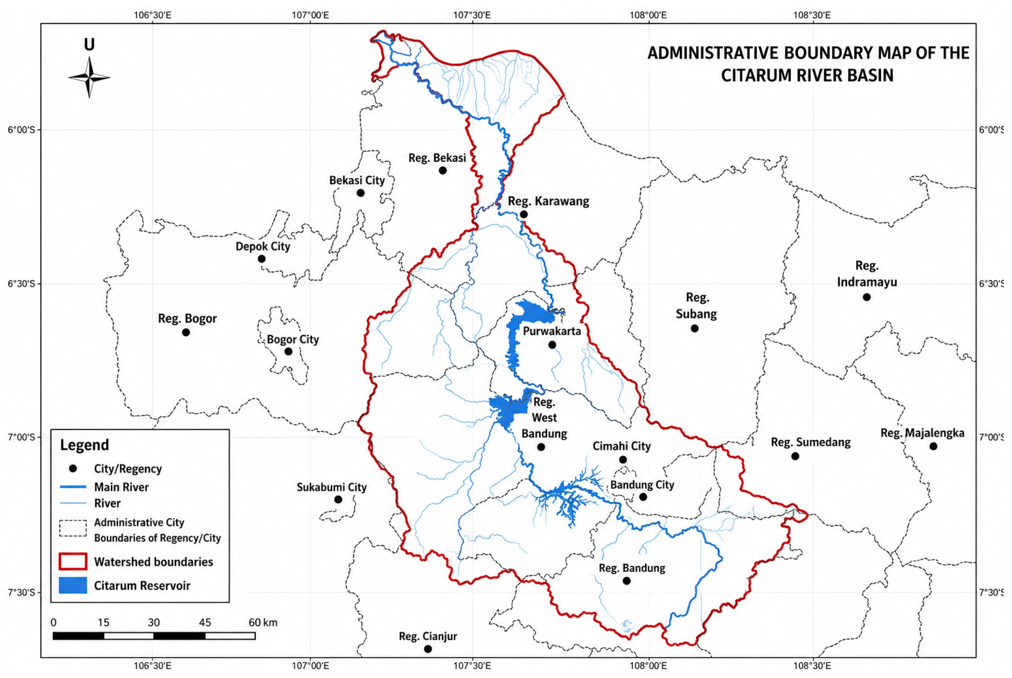
The Citarum River Basin (Derah Aliran Sungai/DAS), located in West Java Province, Indonesia, covers approximately 6614 km² and has a main river extending about 297 km from its mountainous headwaters to downstream lowland regions [1]. As one of the most critical river systems in Indonesia, it supports domestic water supply, irrigation, industrial activities, and hydropower generation for millions of residents. Despite its strategic importance, the basin has experienced substantial environmental degradation driven by sustained anthropogenic pressures, particularly rapid urbanization, industrial expansion, and inadequate waste management practices. The spatial configuration and hydrological boundaries of the study area are illustrated in Figure 1.

Physiographically, the basin exhibits considerable topographic variation, ranging from elevations above 2000 m in upstream areas to approximately 650–750 m in downstream regions. Slope gradients, typically between 5% and 15%, influence runoff processes, settlement distribution, and the potential transport of land-based waste into river systems. Climatically, the basin is characterized by a tropical monsoon regime (Af/Am), with pronounced wet and dry seasons. Annual precipitation ranges from 2000 to 3500 mm, with peak rainfall from November to April, while the dry season (May–October) receives significantly lower rainfall. These seasonal dynamics influence surface runoff and river discharge, which, in turn, affect the mobilization of waste from terrestrial sources into the river system. However, due to the limited availability of high-resolution hydrological data, such variables are not explicitly incorporated into the predictive models and are instead used to provide environmental context for interpreting temporal patterns.

The selection of DAS Citarum is further supported by its relevance to data-driven modeling under constrained conditions. The basin exhibits strong spatial heterogeneity, with relatively less disturbed upstream regions and densely populated, industrialized midstream and downstream areas. This combination of environmental complexity and limited data availability makes the basin a suitable case for developing proxy-based modeling approaches. From a systems perspective, the basin functions as an interconnected hydrological unit, where waste generated across different regions can be transported through drainage networks to downstream areas. These conditions justify the use of a basin-scale analytical perspective to capture aggregated waste generation proxies rather than localized physical transport processes.

In this context, this study adopts a quantitative, data-driven research design to model waste dynamics using a proxy-based time-series framework. The analysis relies on reconstructed daily waste volume data derived from official municipal statistics, which are explicitly treated as indirect indicators rather than direct measurements of riverine waste transport. This approach reflects common data limitations in developing regions while enabling systematic exploration of temporal patterns through machine learning techniques.

The analytical framework is organized into four sequential and interrelated stages. The first stage involves data acquisition and preprocessing, including data cleaning, unit standardization, and temporal alignment. Particular attention is given to ensuring dataset reliability and establishing a robust baseline for reconstruction.

The second stage focuses on exploratory temporal analysis and feature engineering. Temporal features, including lag variables, rolling statistics, and seasonal indicators, are examined to understand the internal structure of the reconstructed proxy dataset. This stage is crucial for encoding the temporal dependencies that drive the predictive models.

The third stage consists of model development and validation using supervised machine learning approaches, specifically Random Forest, Support Vector Regression (SVR), Extreme Gradient Boosting (XGBoost), and Long Short-Term Memory (LSTM). The dataset is split chronologically into training (80%) and testing (20%) subsets to preserve temporal dependencies. Importantly, a time-aware validation strategy is implemented, with all data transformations and feature engineering applied strictly within the training set to prevent data leakage and ensure the model’s external validity.

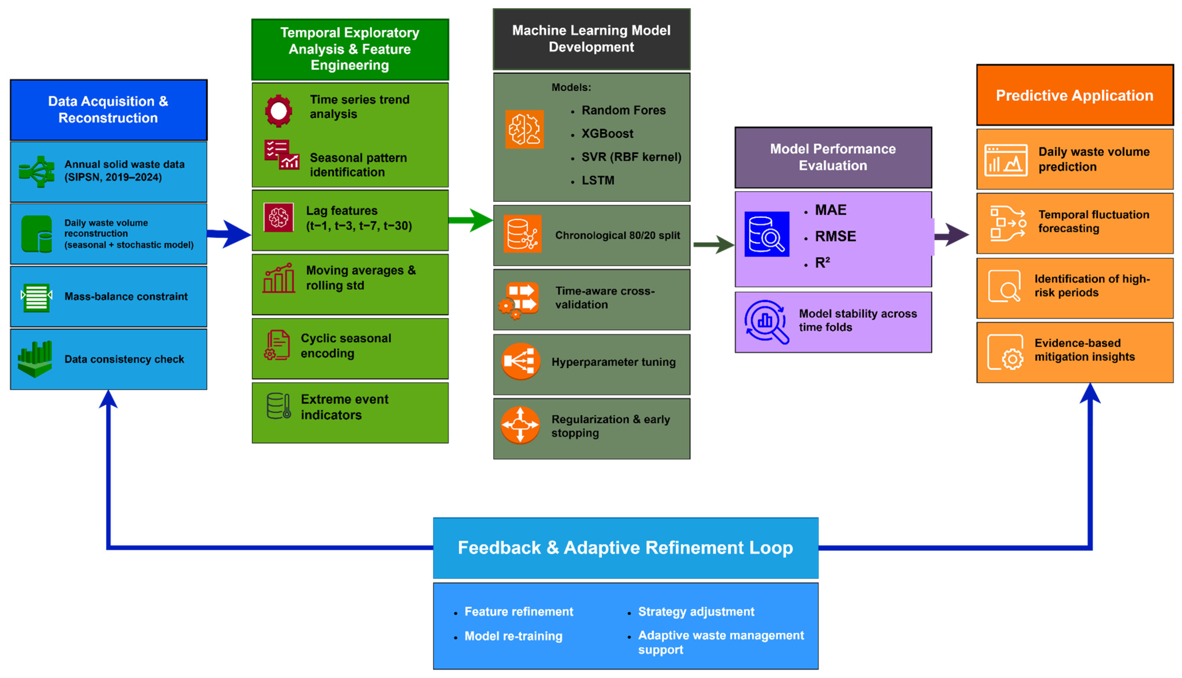
The final stage involves predictive evaluation and performance assessment. Model outputs are compared against the observed values in the test set using multiple metrics, including Mean Absolute Error (MAE), Root Mean Square Error (RMSE), and the coefficient of determination (R²). The overall workflow of the study is illustrated in Figure 2.

2.2. Data Acquisition and Sources

The data used in this study were obtained from the National Waste Management Information System (Sistem Informasi Pengelolaan Sampah Nasional/SIPSN) for the 2019–2024 period, covering administrative regions within DAS. The dataset was accessed through the official SIPSN portal (https://portal-sipsn.kemenlh.go.id/ accessed on 15 Jauary 2026) managed by the Ministry of Environment and Forestry on 15 January 2026. As a government-managed reporting platform, SIPSN serves as the primary national reference for evaluating municipal solid waste management performance in Indonesia.

The dataset consists of aggregated annual waste generation statistics, reported at the municipal level. These data are systematically collected and publicly accessible. However, they are temporally coarse and spatially heterogeneous. This reflects differences in reporting practices, monitoring frequency, and data completeness across regions. As a result, the dataset does not directly support high-resolution temporal analysis or time-series forecasting without further processing. This limitation is common in many environmental datasets in developing regions and is a central methodological challenge addressed in this study.

To enable temporal modeling, a reconstruction procedure was implemented to generate a synthetic daily time series that is fully constrained by the officially reported annual totals. The reconstructed dataset is denoted as $\left\{V_t{\}}_{t=1}^N\right.$, where $V_t$ represents the estimated waste volume on day $t$, and $N$ is the number of days in a given year. Importantly, the reconstructed values are not independent observations but are generated within a constrained system such that:

• the sum of all daily values equals the reported annual total;
• temporal structure is imposed through deterministic and stochastic components.

This formulation explicitly frames the dataset as a proxy-based representation, rather than a direct measurement of riverine waste dynamics.

The reconstruction process employs an additive seasonal–stochastic model, defined as:

$$V_t=S_t+{\epsilon }_t,$$

(1)

where $S_t$ represents the deterministic seasonal component and ${\epsilon }_t\sim \mathcal{N}(0,{\sigma }^2)$ captures stochastic daily variability. This structure is selected to reflect two key characteristics of waste generation systems: (i) the presence of recurring seasonal patterns associated with socio-economic and climatic cycles, and (ii) short-term fluctuations driven by operational and behavioral variability.

The seasonal component $S_t$ is constructed using five control points within each annual cycle: the beginning of the year, the first seasonal peak, the mid-year minimum, the second seasonal peak, and the end of the year. These control points are denoted as $\left(t_1,S_1),(t_2,S_2),(t_3,S_3),(t_4,S_4),(t_5,S_5\right)$, where $t_1=1$ and $t_5=N$. The intermediate points define a bi-modal seasonal structure, consistent with patterns often observed in monsoon-influenced regions.

Intermediate daily values are estimated using a modified piecewise linear interpolation scheme:

$$S_t=S_i+\left(S_{i+1}-S_i\right)\cdot {\displaystyle \frac{t-t_i}{t_{i+1}-t_i}},$$

(2)

where $S_t$ represents the estimated value at time $t$, $S_i$ is the observed value at time $t_i$, and $S_{i+1}$ denotes the observed value at time $t_{i+1}$. In this classical expression, the term ${\displaystyle \frac{S_{i+1}-S_i}{t_{i+1}-t_i}}$ describes the rate of change between two consecutive observations, while $\left(t−t_i\right)$ indicates the time distance from the initial observation. This formulation is widely used for estimating intermediate values under the assumption that the change between two known data points follows a linear pattern, as commonly discussed in time-series interpolation literature [28].

To capture the effects of varying seasonal intensities and inherent structural variability in waste generation, a seasonal weighting parameter $\alpha$ was incorporated into the interpolation scheme:

$$S_t=S_i+\alpha \cdot (S_{i+1}-S_i)\cdot {\displaystyle \frac{t-t_i}{t_{i+1}-t_i}},$$

(3)

The inclusion of $\alpha$ enables modulation of the interpolation slope according to seasonal characteristics, improving the model’s capacity to retain abrupt changes without introducing artificial smoothing. This approach follows the principles of adaptive piecewise representations in time-series analysis, where segment-specific adjustments are applied to capture dynamic patterns in the data [29]. By providing this flexibility, the interpolation preserves sudden seasonal transitions while avoiding over-smoothing, which is particularly crucial for representing non-uniform seasonal behavior in reconstructed environmental time series.

The stochastic component is incorporated as:

$${ϵ}_t=\sigma \cdot Z_t,$$

(4)

where $Z_t\sim N\left(\mathrm{0,1}\right)$ and $\sigma$ denotes the standard deviation controlling daily fluctuations. This term introduces high-frequency variability, generating realistic day-to-day variations while maintaining alignment with the seasonal structure. To ensure consistency with reported annual totals, a global scaling adjustment is applied after reconstruction. Boundary conditions are also enforced by fixing the first and last observations ($S_1,S_n$), thereby preserving temporal coherence across consecutive years.

It is important to note that this reconstruction approach inherently introduces structural assumptions and uncertainty, as the generated daily values are not directly observed. Consequently, the resulting dataset should be regarded as a synthetic yet constrained proxy, intended to approximate plausible temporal dynamics under limited data availability. This limitation has implications for model generalizability and is explicitly acknowledged throughout the study.

2.3. Data Preprocessing and Quality Control

Data preprocessing and quality control are critical stages for ensuring the validity, robustness, and reproducibility of the proposed machine learning framework. Given that the dataset is derived from a reconstructed daily time series based on annual municipal solid waste statistics, preprocessing is designed to ensure temporal consistency, statistical stability, and methodological rigor, while explicitly addressing potential biases inherent in proxy-based data.

Initial validation procedures were conducted to ensure consistency in variable definitions, measurement units, and temporal indexing. All waste-related variables were standardized into consistent units of tons per day (t/day) during pre-processing to ensure comparability across temporal observations and to eliminate unit-related inconsistencies. In addition, the reconstructed dataset was systematically verified to satisfy imposed structural constraints, including preservation of annual totals, boundary conditions at the beginning and end of each year, and continuity of the daily time index. These steps ensure internal coherence and prevent structural inconsistencies that could compromise downstream analysis [30,31].

Although the reconstruction procedure generates a complete daily series by design, missing values may still arise due to numerical precision adjustments, rounding operations, or transformations introduced during feature engineering. To preserve temporal continuity, missing values in time-dependent variables were handled using linear interpolation. Consistent with standard interpolation approaches and reviewer recommendations, the formulation is defined as:

$$w_t=0.5\left(w_{t+1}+w_{t-1}\right),$$

(5)

where $w_t$ denotes the estimated value at time $t$, and $w_{t-1}$ and $w_{t+1}$ represent adjacent observations. This formulation ensures local consistency while avoiding artificial distortion of temporal dynamics. The use of interpolation is intentionally limited and carefully controlled to prevent excessive smoothing of the reconstructed signal.

For non-temporal or weakly time-dependent variables, statistical imputation was applied using measures of central tendency:

$$x_{\mathrm{rep}}=\left\{\begin{array}{cc}\overline{x},& \mathrm{for}\mathrm{skewed}\mathrm{distributions}\left(\mathrm{Median}\right)\\ \tilde{x},& \mathrm{for}\mathrm{symmetric}\mathrm{distributions}\left(\mathrm{Mean}\right)\end{array}\right.,$$

(6)

where $\overline{x}$ and $\tilde{x}$ denote the mean and median, respectively. The choice between these estimators is guided by distributional diagnostics to preserve the intrinsic statistical properties of each variable [32].

Outlier detection was performed using the standardized z-score criterion:

$$z={\displaystyle \frac{x-\mu }{\sigma }},$$

(7)

where $x$ is the observed value, $\mu$ is the mean, and $\sigma$ is the standard deviation. Observations satisfying $\mid z\mid >3$ were flagged as potential outliers. However, given the inherent variability of environmental systems and the stochastic nature of the reconstructed dataset, extreme values representing plausible system dynamics were retained. Only anomalous values resulting from numerical artifacts were adjusted using winsorization, thereby reducing their influence without compromising the structural integrity of the dataset [33,34].

To ensure numerical stability and scale invariance across features with differing magnitudes, all numerical variables were normalized using min–max scaling [31,35]:

$$x^{\prime }={\displaystyle \frac{x-x_{\mathrm{m}\mathrm{i}\mathrm{n}}}{x_{\mathrm{m}\mathrm{a}\mathrm{x}}-x_{\mathrm{m}\mathrm{i}\mathrm{n}}}}.$$

(8)

where $x^{\prime }$ is the normalized value of the variable $x$, $x$ represents the original data value, $x_{\mathrm{m}\mathrm{i}\mathrm{n}}$ denotes the minimum value in the dataset, and $x_{\mathrm{m}\mathrm{a}\mathrm{x}}$ is the maximum value in the dataset. This formula is used for min–max normalization, which rescales data into a range be-tween 0 and 1 to ensure comparability and stability in data analysis and machine learning models. To strictly avoid data leakage, all normalization parameters were computed exclusively on the training dataset and subsequently applied to the testing dataset. This ensures that no information from future observations is introduced during model training.

Temporal harmonization was then applied to align all variables and engineered features on a consistent daily resolution. The dataset was partitioned chronologically, with the first 80% of observations allocated to the training set and the remaining 20% reserved for testing. All preprocessing operations including interpolation, normalization, and feature transformations were performed exclusively on the training subset, with learned parameters transferred to the testing subset. This time-aware strategy preserves temporal dependencies and prevents information leakage, ensuring that model evaluation reflects realistic forecasting conditions [36].

To further address concerns regarding dataset representativeness, additional statistical checks were conducted to evaluate distributional stability and temporal consistency across the study period. Descriptive statistics, interannual variability, and distributional characteristics were examined to ensure that the reconstructed dataset captures plausible variability patterns without introducing artificial bias. While these analyses do not fully substitute for real observational data, they provide quantitative support for the internal consistency of the dataset.

It is important to emphasize that the reconstructed time series represents a proxy approximation derived from aggregated statistics rather than direct riverine measurements. Consequently, the dataset primarily captures temporal patterns of potential waste generation. This approach allows for model development under data-constrained conditions, acknowledging that while it provides a data-driven approximation, it does not explicitly model physical in-stream transport processes.

Furthermore, hydrological and climatic drivers such as river discharge, precipitation, and flow velocity are not explicitly incorporated into the modeling framework due to data unavailability at the required temporal resolution. Instead, temporal features such as seasonality, lag effects, and extreme-value indicators are assumed to implicitly capture part of these dynamics. While this assumption enables model development under data-constrained conditions, it also limits the physical interpretability and generalizability of the results.

2.4. Feature Engineering and Selection

Feature engineering and selection were designed to transform the reconstructed daily waste volume time series into informative predictors that capture temporal dynamics, system memory, and seasonal variability within DAS Citarum. Given the absence of high-resolution hydrological, meteorological, and socio-economic observations, all features were derived exclusively from the reconstructed waste volume series. Therefore, the modeling framework should be interpreted as a proxy-based temporal learning system, where the model captures internal statistical structure rather than explicitly simulating physical waste transport processes.

Temporal dependencies and system memory were incorporated through lagged features of daily waste volume, generically expressed as $V_{t-k}$ with $k\in \{\mathrm{1,3},\mathrm{7,14}\}$. These features capture short- to medium-term persistence effects associated with accumulation and release processes inherent in urban waste management systems. In addition, rolling statistics were computed to characterize the background state of the system over multiple temporal scales.

To characterize the evolving background state of the system, rolling statistical features were computed over multiple time windows. The moving average is defined as [37]:

$${\mathrm{M}\mathrm{A}}_n(t)={\displaystyle \frac{1}{n}}{\displaystyle \sum _{i=0}^{n-1}}{V}_{t-i},$$

(9)

where $M{A}_n\left(t\right)$ denotes the moving average of order $n$ at time $t$, $n$ represents the number of observations included in the averaging window, and $V_{t-i}$ is the value of the variable $V$ at time $t-i$. The summation term ${\sum }_{i=0}^{n-1}{V}_{t-i}$ calculates the total of the most recent $n$ observations, and dividing by $n$ yields the average, which is used to smooth short-term fluctuations in time series data.

The moving standard deviation over a sliding window of size $w$ is defined as follows:

$${\sigma }_t=\sqrt{{\displaystyle \frac{1}{w-1}}{\displaystyle \sum _{i=t-w+1}^t}{\left(x_i−{\overline{x}}_t\right)}^2},$$

(10)

where ${\sigma }_t$ denotes the moving (rolling) standard deviation at time $t$, $w$ is the window size, $x_i$ represents the observed value at time $i$, and ${\overline{x}}_t$ is the mean of the observations within the window from $t-w+1$ to $t$. The term $w-1$ is used to provide an unbiased estimate of variability. These features were calculated using 3-day, 7-day, and 30-day windows to capture short-term fluctuations, weekly variability, and monthly trends, respectively. Such multi-scale representation enables the model to learn both local volatility and broader temporal patterns embedded in the reconstructed dataset.

Seasonal variability was incorporated using cyclic temporal encoding to preserve continuity across annual boundaries. Calendar months were transformed into sine and cosine components:

$${\mathrm{M}\mathrm{o}\mathrm{n}\mathrm{t}\mathrm{h}}_{\mathrm{s}\mathrm{i}\mathrm{n}}=\mathrm{s}\mathrm{i}\mathrm{n}\left({\displaystyle \frac{2\pi \cdot \mathrm{month}}{12}}\right), {\mathrm{M}\mathrm{o}\mathrm{n}\mathrm{t}\mathrm{h}}_{\mathrm{c}\mathrm{o}\mathrm{s}}=\mathrm{c}\mathrm{o}\mathrm{s}\left({\displaystyle \frac{2\pi \cdot \mathrm{month}}{12}}\right),$$

(11)

ensuring that December–January transitions are represented smoothly. In addition, a binary seasonal indicator (wet vs. dry season) was included to indirectly capture monsoonal influences, which are known to affect waste mobilization processes, even though hydrological variables were not explicitly modeled.

Extreme conditions in the waste volume time series, potentially reflecting large-scale accumulation or release events, were captured using threshold-based indicators defined as:

$$E_V=\left\{\begin{array}{cc}1,& V_t>\mu +2\sigma ,\\ 0,& \mathrm{otherwise},\end{array}\right.,$$

(12)

where $\mu$ and $\sigma$ denote the long-term mean and standard deviation of daily waste volume, respectively. This feature identifies high-intensity events that may disproportionately influence system dynamics and model learning.

Feature selection was conducted using a sequential multi-criteria approach to balance predictive power and model parsimony. First, Pearson and Spearman correlation analyses were applied to identify highly collinear feature pairs, with the correlation coefficient defined as [33]:

$$r={\displaystyle \frac{\sum (x_i-\overline{x})(y_i-\overline{y})}{\sqrt{\sum (x_i-\overline{x}{)}^2\sum (y_i-\overline{y}{)}^2}}},$$

(13)

where $x_i$ and $y_i$ represent paired observations, and $\overline{x}$ and $\overline{y}$ denote their respective means. Features with $\mid r\mid >0.8$ were considered redundant and excluded. In addition, Spearman rank correlation was employed to detect monotonic but non-linear relationships between variables.

Subsequently, feature importance rankings were obtained using a Random Forest model as a wrapper-based selection mechanism. Finally, recursive feature elimination (RFE) combined with time-aware cross-validation was applied exclusively to the training dataset to determine the optimal subset of predictors, thereby ensuring that feature selection did not introduce information leakage into the testing phase.

The final feature set consisted of 18 predictors, including selected lag variables (e.g., $V_{t-1},V_{t-3},V_{t-7}$), rolling statistics (e.g., 7-day moving average and 30-day standard deviation), seasonal encodings, and extreme-event indicators. Feature importance analysis indicated that short-term lag variables and rolling averages contributed most significantly to model performance, highlighting the dominant role of intrinsic temporal structure in the reconstructed dataset.

It is important to emphasize that, due to the absence of independent environmental drivers, the resulting model prioritizes statistical predictability over physical interpretability. Therefore, model outputs should be interpreted as forecasts of proxy waste dynamics rather than direct representations of riverine waste transport. This limitation underscores the need for future integration of hydrological, climatic, and socio-economic variables to improve model generalizability and strengthen its applicability in real-world environmental management contexts.

2.5. Machine Learning Models

2.5.1. Model Description

This study employs four machine learning algorithms RF, XGBoost, SVR, and LSTM to model the nonlinear and temporal dynamics of reconstructed daily waste volume in the Citarum River Basin. It is important to emphasize that the target variable represents a proxy-based time series derived from annual waste statistics; therefore, the models primarily learn temporal structures embedded in the reconstructed data rather than directly observed riverine processes.

The selected models represent complementary learning paradigms, enabling a comparative evaluation of predictive performance under data-limited conditions. To ensure clarity and conciseness, only the key characteristics of each model are presented, while detailed algorithmic descriptions are omitted as they are well established in the literature.

• Random Forest (RF);

RF is an ensemble-based method that combines multiple decision trees built using bootstrap sampling and random feature selection. For regression tasks, predictions are obtained by averaging across trees [13,33]:

$$\widehat{y}(x)={\displaystyle \frac{1}{T}}{\displaystyle \sum _{t=1}^T}{h}_t(x),$$

(14)

where $h_t\left(x\right)$ denotes the prediction of the $t$-th tree and $T$ is the total number of trees. This aggregation reduces variance and enhances robustness, making RF suitable for capturing nonlinear relationships among engineered temporal features. In addition, RF provides feature importance estimates that support model interpretability.

2.

Support Vector Regression (SVR);

SVR is a kernel-based regression approach that estimates a function within an $\epsilon$-insensitive margin while controlling model complexity. In this study, the radial basis function kernel is used to model nonlinear relationships [30]:

$$K\left(x_i,x_j\right)=\exp \left(-\gamma \parallel x_i-x_j{\parallel }^2\right).$$

(15)

SVR is particularly suitable for moderate-sized datasets and provides stable generalization performance.

3.

Long Short-Term Memory (LSTM);

Long Short-Term Memory networks are a class of recurrent neural networks specifically designed to model long-range temporal dependencies in sequential data. LSTM architectures employ gating mechanisms to regulate information flow across time steps, defined as [35]:

$$f_t=\sigma \left(W_f[h_{t-1},x_t]+b_f\right),$$

(16)

$$i_t=\sigma \left(W_i[h_{t-1},x_t]+b_i\right),$$

(17)

$${\tilde{c}}_t=\tanh \left(W_c\left[h_{t-1},x_t\right]+b_c\right),$$

(18)

$$c_t=f_t\odot c_{t-1}+i_t\odot {\tilde{c}}_t,$$

(19)

$$o_t=\sigma \left(W_o[h_{t-1},x_t]+b_o\right),$$

(20)

$$h_t=o_t\odot \tanh \left(c_t\right),$$

(21)

where $x_t$ denotes the input vector at time $t$, $h_t$ the hidden state, and $c_t$ the cell state. This architecture enables LSTM models to capture delayed effects, accumulation behavior, and long-term seasonal patterns inherent in daily waste volume time series, which are difficult to represent using static regression models or shallow learning approaches.

4.

Extreme Gradient Boosting (XGBoost).

XGBoost is the primary model of this study due to its strong predictive performance and robustness. It is a regularized gradient boosting framework that sequentially builds decision trees to minimize prediction error while controlling model complexity [38,39]. The objective function at iteration $t$ is defined as:

$${\mathcal{L}}^{\left(t\right)}=\sum _{i}l\left({\widehat{y}}_i^{\left(t−1\right)}+f_t(x_i),y_i\right)+\Omega (f_t),$$

(22)

where $l(\cdot )$ denotes the loss function and $\Omega (f_t)$ is a regularization term. Using second-order approximation, the optimization is expressed as:

$${\mathcal{L}}^{\left(t\right)}\approx \sum _i\left[g_i{f}_t(x_i)+{\displaystyle \frac{1}{2}}{h}_i{f}_t^2(x_i)\right]+\Omega (f_t),$$

(23)

where $g_i$ and $h_i$ represent first- and second-order gradients. This formulation enables efficient learning of complex nonlinear interactions among engineered temporal features.

2.5.2. Model Configuration

The model configurations were designed to ensure a fair comparison, robust generalization, and strict preservation of the dataset’s temporal structure. Given that the target variable represents a reconstructed daily time series derived from annual statistics, particular attention was devoted to mitigating overfitting to synthetic temporal patterns and to preventing data leakage. All transformations were strictly confined to the training data to eliminate potential information leakage.

A chronological split was adopted, with 80% of the observations used for training and the remaining 20% reserved for out-of-sample testing. All preprocessing steps, including normalization and feature scaling, were fit exclusively to the training set and subsequently applied to the validation and test sets. Hyperparameter tuning was conducted using a rolling-origin cross-validation scheme, ensuring that validation folds always follow the corresponding training data in temporal order. This approach reflects realistic forecasting conditions and preserves the integrity of time-series dependencies.

Different optimization strategies were employed depending on model complexity. Grid search was applied to RF and SVR, while Bayesian optimization was used for XGBoost and LSTM to efficiently explore higher-dimensional hyperparameter spaces. Hyperparameters were selected based on validation performance averaged across time-ordered folds, with emphasis on stability rather than solely on maximizing predictive accuracy, to reduce sensitivity to reconstruction-induced artifacts.

The final hyperparameter configurations were selected based on consistent performance across cross-validation folds. Increasing model complexity beyond the selected values generally did not yield meaningful improvements in validation performance while increasing the risk of overfitting. These configurations, therefore, represent a balanced trade-off between model flexibility and generalization under reconstructed-data conditions. The optimized configurations are summarized in

Table 1. Model configuration, hyperparameter search space, and computational setup.

Model	Hyperparameter	Final Value	Data-Specific Justification
RF	Number of trees (T)	320	Validation performance plateau observed beyond moderate ensemble size
	Max depth	14	Larger depth increased sensitivity to reconstructed seasonal fluctuations
	Min samples split	3	Improved stability under sparse daily variability
	Min samples leaf	2	Reduced sensitivity to synthetic noise fluctuations
	Max features	log2	Increased diversity under correlated temporal predictors
XGBoost	Number of estimators (max)	280	Upper bound; actual iterations determined by early stopping on internal validation set
	Learning rate	0.045	Controlled learning dynamics under seasonal variability
	Max depth	5	Prevented overfitting to short-term lag artifacts
	Subsample	0.82	Reduced dependency on repeated temporal structures
	Colsample_bytree	0.78	Controlled redundancy from lag-based features
	Gamma (γ)	0.15	Regularized split decisions under synthetic variations
	Lambda (λ)	1.2	Stabilized model under limited variability
	Alpha (α)	0.05	Promoted sparsity in redundant temporal features
	Early stopping rounds	20	Training halted when validation loss does not improve over 20 consecutive iterations
	Internal validation fraction	15% of training set	Final 15% of chronological training partition reserved for early stopping; test set remains unseen
SVR	Kernel	RBF	Captures nonlinear temporal relationships
	C (penalty)	12	Balanced bias–variance trade-off under reconstructed data
	Gamma (γ)	0.008	Prevented overly complex decision boundaries
	Epsilon (ε)	0.08	Reduced sensitivity to artificial noise
LSTM	Hidden units	72	Larger units increased training instability
	Number of layers	2	Deeper architectures led to rapid overfitting
	Sequence length	12 days	Captured short-term dependency without noise accumulation
	Dropout rate	0.25	Regularization against synthetic temporal patterns
	Learning rate	0.0008	Ensured stable gradient updates
	Batch size	48	Provided stable convergence across folds
	Epochs	Max 100 (early stopping)	Early stopping applied based on validation loss (patience = 10) to prevent overfitting

and were consistently used in all subsequent experiments, ensuring reproducibility and fair benchmarking across models.

A critical methodological correction was applied to the XGBoost training procedure. In the original implementation, the early stopping evaluation set inadvertently referenced the held-out test partition, resulting in data leakage that artificially inflated reported test performance. This was corrected by constructing the internal validation set exclusively from the final 15% of the chronological training partition, leaving the test set entirely unseen throughout all training and model selection procedures. As a consequence of this correction, the effective number of boosting iterations is governed by best_iteration rather than the nominal maximum of 280, and the corrected test performance reflects genuine out-of-sample generalization. This finding reinforces the recommendations of Meyer et al. [22] regarding the necessity of strict temporal data partitioning in time-series modeling contexts.

2.6. Model Training and Validation Strategy

Model training in this study follows a time-series–aware learning framework designed to preserve temporal dependencies and causal structure inherent in reconstructed daily waste volume dynamics at the watershed scale. Observations ${\left\{(X_t,y_t)\right\}}_{t=1}^T$ were strictly ordered in time, and all models were trained to learn the mapping ${\widehat{y}}_t=f(X_t;\theta )$ using only past information. This design eliminates look-ahead bias and ensures that model development reflects realistic forecasting conditions.

To address non-stationarity, serial correlation, and seasonal variability embedded in the reconstructed time series, time-aware validation strategies were employed instead of conventional random k-fold cross-validation. Specifically, a rolling-origin evaluation scheme was implemented, in which the training set expands progressively while the validation window moves forward in time:

$${\mathrm{Train}}_i=\{1,\dots ,t_i\},{\mathrm{Validate}}_i=\{t_i+1,\dots ,t_i+h\},$$

(24)

where $h$ denotes the validation horizon. In addition, blocked cross-validation was applied by partitioning the dataset into contiguous temporal segments to ensure strict separation between training and validation sets $\left({\mathrm{Train}}_i\cap {\mathrm{Validate}}_i=\mathrm{\varnothing }\right)$. These complementary strategies provide unbiased performance estimates and prevent information leakage in temporally structured data [38].

Overfitting control was implemented through model-specific regularization mechanisms. For tree-based models (RF and XGBoost), model complexity was constrained by limiting tree depth, minimum samples per split, and feature subsampling. In XGBoost, regularization was further enforced through penalties on tree complexity and leaf weights, expressed as $\Omega (f_k)=\gamma T_k+{\displaystyle \frac{1}{2}}\lambda \parallel w_k{\parallel }^2$. For SVR, generalization was controlled via the regularization parameter $C$, kernel width $\gamma$, and the $ϵ$-insensitive loss function. For LSTM, dropout regularization (rate = 0.25) and early stopping were applied, with training halted when validation loss failed to improve over $p=10$ consecutive epochs, ensuring that model selection was based on the optimal generalization point rather than final training iterations.

To address potential data leakage during early stopping, model-specific validation partitioning was applied as follows. For LSTM, an internal validation split of 15% was applied via Keras’ built-in validation_split parameter, drawing observations from the end of the training sequence. For XGBoost, an analogous early stopping mechanism was applied with a patience of 20 boosting iterations. Critically, the internal validation set for XGBoost was constructed exclusively from the final 15% of the chronological training partition—not from the held-out test set—ensuring that the test set remained entirely unseen throughout all training and model selection procedures. As a result, XGBoost is effectively trained on 85% of the training partition (approximately 68% of the total dataset), whereas RF and SVR, which do not employ early stopping, use the full 80% training partition for model fitting. This difference is acknowledged as a minor but necessary consequence of the corrected validation protocol, and is explicitly reported to ensure methodological transparency [22].

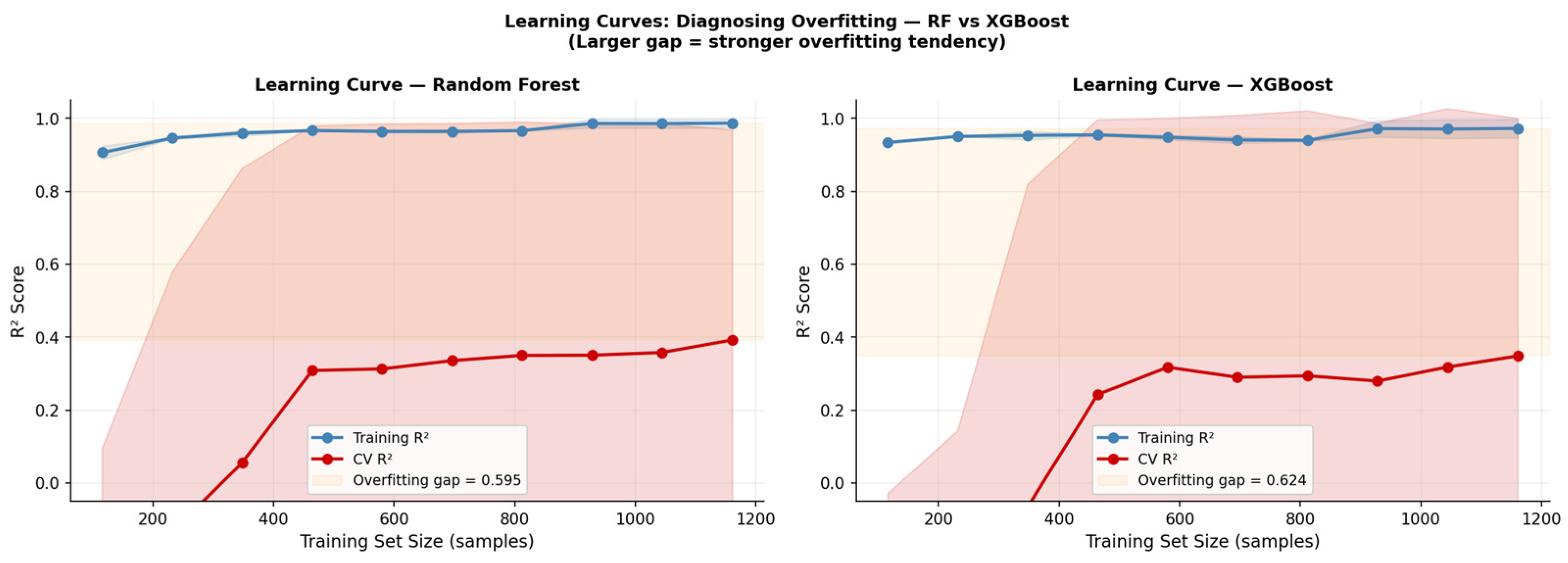
To explicitly diagnose and control underfitting and overfitting, the trajectories of training and validation errors were systematically analyzed. Overfitting was identified when training error continued to decrease while validation error increased or became unstable in later training stages, indicating memorization of noise rather than generalizable patterns. In contrast, underfitting was characterized by persistently high errors in both training and validation sets, reflecting insufficient model capacity or inadequate feature representation. In such cases, model configurations were iteratively refined through hyperparameter tuning and feature enhancement. To complement this analysis, learning curves were used to quantitatively assess the gap between training and cross-validation R² for RF and XGBoost, providing both visual and numerical evidence of their differing generalization behavior. Figure 3 illustrates these learning dynamics and highlights the stronger overfitting tendency observed in RF compared to XGBoost.

Based on Figure 3, both models exhibit clear overfitting, characterized by very high and stable training R² values (close to 1), while the cross-validation (CV) R² is much lower. In RF, the training curve increases rapidly and then plateaus around 0.98–0.99, while the validation curve increases gradually but remains in a much lower range (around 0.30–0.39), resulting in an overfitting gap of 0.595. A similar pattern is also seen in XGBoost, where the training R² stabilizes in the high range (~0.95–0.97), while the validation R² is in the lower range (~0.25–0.35), with an even slightly larger gap (0.624). Although both models show improved validation performance as the training data size increases, the consistent gap between the training and validation curves indicates that they are still capturing specific patterns of the training data that are not fully generalized. Comparatively, XGBoost shows a slightly stronger tendency to overfitting than RF, as reflected by the larger gap, although both still suffer from generalization limitations under noisy data and reconstructed results.

Given that the dataset is reconstructed from annual statistics using a seasonal–stochastic process, additional care was taken to prevent models from over-learning synthetic temporal patterns. Regularization strength, model complexity, and validation stability were jointly considered during model selection to ensure that learned representations reflect generalizable temporal structures rather than reconstruction-specific artifacts.

2.7. Performance Evaluation Metrics

2.7.1. Mean Absolute Error (MAE)

MAE measures the average magnitude of absolute differences between predicted and observed values, expressed in the same units as the target variable (t/day). MAE is defined as [40]:

$$\mathrm{MAE}={\displaystyle \frac{1}{n}}{\displaystyle \sum _{i=1}^n}\mid y_i-{\widehat{y}}_i\mid ,$$

(25)

where $y_i$ denotes the observed waste volume, ${\widehat{y}}_i$ the corresponding model prediction, and $n$ the number of test samples. Owing to its intuitive interpretation and linear error penalization, MAE is particularly useful for operational decision-making and stakeholder-oriented assessments of forecasting reliability [40].

2.7.2. Root Mean Square Error (RMSE)

RMSE quantifies the square root of the mean squared prediction error and assigns greater weight to large deviations between predicted and observed values. RMSE is computed as [41]:

$$\mathrm{RMSE}=\sqrt{{\displaystyle \frac{1}{n}}{\displaystyle \sum _{i=1}^n}(y_i-{\widehat{y}}_i{)}^2},$$

(26)

This metric is especially relevant for hydrological and waste transport applications, where large prediction errors during flood-induced waste surges may result in disproportionate environmental and management impacts [41].

2.7.3. Mean Absolute Percentage Error (MAPE)

MAPE is employed to quantify the relative magnitude of prediction errors in percentage terms, thereby facilitating intuitive interpretation and cross-model comparison. MAPE measures the average absolute deviation between predicted and observed values relative to the observed values and is formulated as:

$$\mathrm{MAPE}={\displaystyle \frac{100}{n}}{\displaystyle \sum _{i=1}^n}\mid {\displaystyle \frac{y_i-{\widehat{y}}_i}{y_i}}\mid ,$$

(27)

where $y_i$ denotes the observed value, ${\widehat{y}}_i$ represents the corresponding predicted value, and $n$ is the total number of observations. To avoid numerical instability, observations with $y_i\approx 0$ were excluded or handled with a small constant adjustment. MAPE enables scale-independent comparison across temporal regimes and is useful for interpreting proportional forecasting errors.

2.7.4. Coefficient of Determination (R²)

R² measures the proportion of variance in the observed data explained by the model [34]:

$$R^2=1-{\displaystyle \frac{{\displaystyle {\sum }_{i=1}^n}(y_i-{\widehat{y}}_i{)}^2}{{\displaystyle {\sum }_{i=1}^n}(y_i-\overline{y}{)}^2}},$$

(28)

where $\overline{y}$ is the mean of observed values. While higher R² values indicate stronger explanatory power, this metric was interpreted cautiously given the reconstructed nature of the dataset, which may inherently favor models capturing internal temporal structure.

2.7.5. Comparative Evaluation and Model Stability Analysis

All models were evaluated under identical temporal holdout conditions to ensure fair comparison. Models achieving lower MAE, RMSE, and MAPE values alongside higher R² values were considered to exhibit superior predictive performance. Beyond average accuracy, model robustness was assessed through stability analysis across time-series cross-validation folds. Specifically, the variability of performance metrics across validation segments was quantified using standard deviation:

$${\mathrm{Stability}}_m=\sigma \left(m\right),m\in \left\{\mathrm{MAE},\mathrm{RMSE},\mathrm{MAPE},R^2\right\}.$$

(29)

Lower variability indicates greater robustness to seasonal transitions, regime shifts, and reconstruction-induced variability. This additional evaluation layer ensures that selected models are not only accurate but also stable and reliable under temporally varying conditions.

2.7.6. Naive Persistence Baseline and Predictive Skill Score

To contextualize the practical added value of the proposed machine learning models beyond the temporal autocorrelation already embedded in the reconstructed proxy series, a naive persistence baseline is established as the minimum performance benchmark against which all models are evaluated. This baseline predicts the waste volume proxy on day $t$ as equal to the observed proxy value on the preceding day $t-1$:

$${\widehat{y}}_t=y_{t-1}.$$

(30)

This formulation represents the simplest possible forecast that exploits temporal continuity, requiring neither model training nor feature engineering. Any machine learning model that fails to surpass the performance of this benchmark cannot be considered to offer genuine predictive capability beyond trivial temporal persistence. To quantify the relative improvement of each model over this benchmark, the RMSE-based predictive skill score is defined as:

$$\mathrm{Skill}=\left(1−{\displaystyle \frac{{\mathrm{RMSE}}_{\mathrm{model}}}{{\mathrm{RMSE}}_{\mathrm{naive}}}}\right)\times 100\%.$$

(31)

A positive skill score indicates that the model reduces prediction error relative to naive persistence; values exceeding 10% are considered practically significant in environmental time-series forecasting literature [42,43]. A negative skill score indicates that the model performs worse than the naive baseline, suggesting a failure to generalize beyond simple autocorrelation. This comparison is particularly important in the present study, given the dominance of the Lag-1 variable in feature importance analyses, which raises the fundamental question of whether the machine learning models extract substantive temporal structure beyond simple day-to-day continuity. The naive baseline, therefore, serves as an essential methodological safeguard against overinterpretation of model performance metrics evaluated against a synthetic proxy rather than direct field observations.

3. Results

3.1. Statistical Integrity and Distribution of Reconstructed Proxies

Evaluating the statistical integrity of the reconstructed daily waste generation proxies is a critical step in ensuring the validity of the proposed predictive modeling framework. Given that this dataset is derived from aggregated annual statistics, a verification process was performed to ensure that the temporal disaggregation preserves the fundamental characteristics of waste dynamics in the watershed while remaining consistent with official government records.

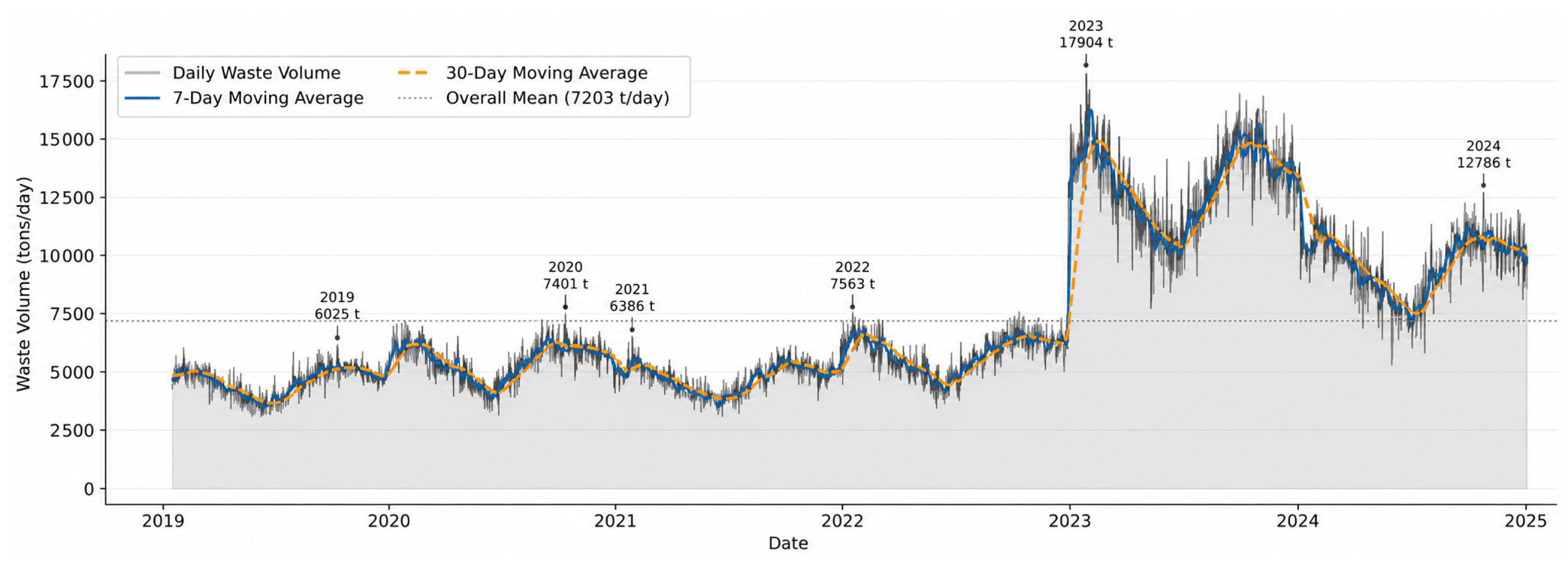
The temporal evolution of the daily waste generation proxies over the six-year study period (2019–2024) is presented in Figure 4. This visualization demonstrates a bimodal seasonal pattern reflecting the interaction between socioeconomic and hydroclimatological factors in the region.

As seen in Figure 4, the time series plot shows a realistic daily fluctuation pattern, generated through a combination of seasonal deterministic and stochastic components $\epsilon$. This approach effectively avoids the artificial smoothing phenomenon common with simple linear interpolation. Furthermore, despite significant daily variations, the accumulated values remain consistent with the annual totals from SIPSN, thus maintaining the dataset’s linkage to the official data source.

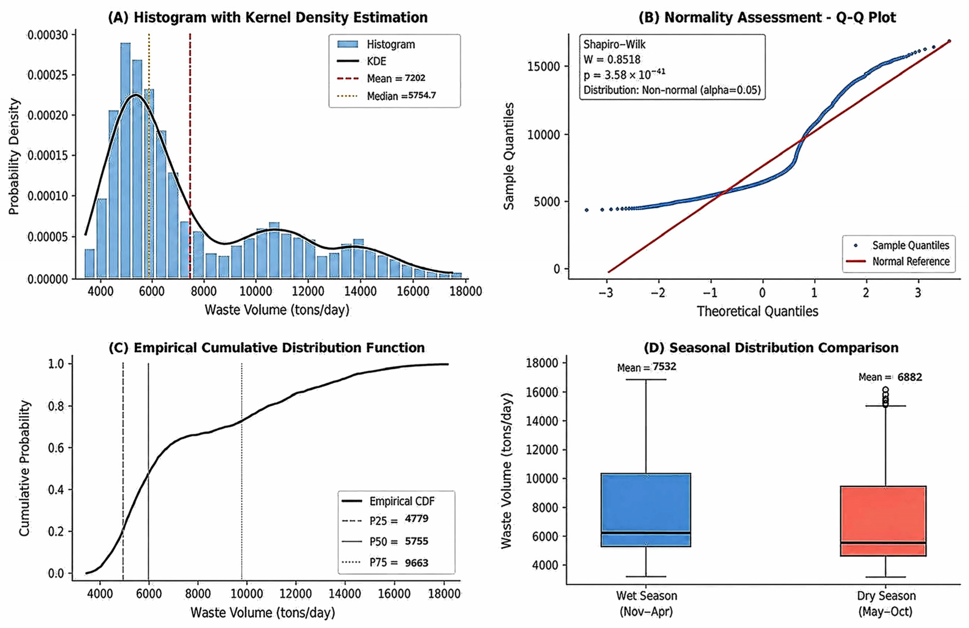
Next, the distribution characteristics of the reconstructed dataset were comprehensively analyzed using the statistical diagnostic panel presented in Figure 5.

Figure 5 shows that the data distribution exhibits a multimodal pattern influenced by interannual variations. Analysis using KDE reveals several peaks in the distribution, while the Q-Q plot and ECDF confirm that, despite a positive skewness, the data still exhibit good statistical continuity without extreme anomalies or significant numerical artifacts. This is crucial for ensuring the stability of the machine learning model training process.

A summary of the numerical characteristics of the daily waste proxy dataset is presented in

Table 2. Annual and overall descriptive statistics of the daily waste volume proxy (2019–2024).

Year	N (Days)	Mean (t/Day)	Median (t/Day)	Std Dev (t/Day)	Min (t/Day)	Max (t/Day)	Skewness	Kurtosis	Total (Tons)	Growth (%)
2019	351	4571.63	4646.52	639.26	3080.70	6025.34	−0.27	−0.51	1,604,642.87	–
2020	366	5460.41	5542.48	833.44	3168.76	7401.24	−0.28	−0.39	1,998,511.64	24.55
2021	365	4698.06	4747.56	642.95	3085.50	6386.34	−0.14	−0.55	1,714,793.30	−14.20
2022	365	5742.87	5810.12	852.58	3447.26	7563.34	−0.27	−0.54	2,096,147.93	22.24
2023	365	13,039.92	13,165.15	1892.33	7707.67	17,904.39	−0.21	−0.40	4,759,570.93	127.06
2024	366	9600.30	9770.70	1377.49	5273.16	12,786.41	−0.36	−0.32	3,513,709.78	−26.18
Total	2178	7202.65	5754.74	3317.30	3080.70	17,904.39	1.064	−0.019	15,687,376	–

.

The reconstructed dataset consists of 2192 daily observations spanning January 2019 to December 2024, with an overall mean of 7187.89 t/day and a standard deviation of 3311.91 t/day. A CV of 46.08% indicates high variability in the daily waste production proxy, underscoring the importance of using machine learning models capable of handling non-stationary time series data.

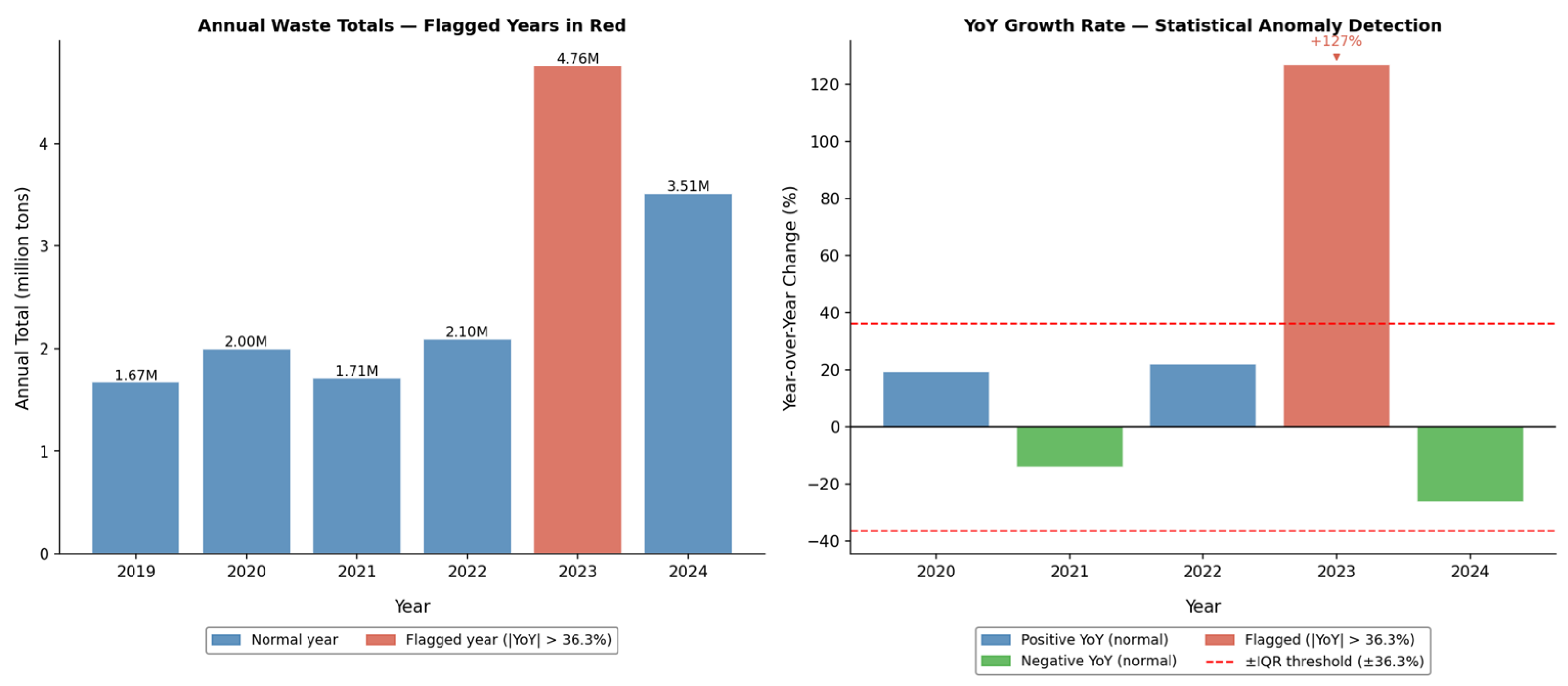
A particularly notable feature of the annual input data is the dramatic increase recorded in 2023, where the official annual total SIPSN increased from 2,096,147.93 tons (2022) to 4,759,570.93 tons, a year-on-year increase of +127.06%. To assess the statistical plausibility of this and other interannual changes, an IQR-based anomaly-detection method was applied to year-on-year percentage changes across all study years. As shown in Figure 6, the IQR anomaly threshold was calculated at ±36.27%, and 2023 was the only year statistically marked as anomalous, with its growth rate exceeding this threshold by approximately 3.5 times. The other years showed growth rates within the expected range, ranging from −26.18% (2024) to +22.24% (2022). The magnitude of the sudden increase in 2023 may reflect an expansion in the geographic coverage of SIPSN reporting, a revision to the municipal waste accounting methodology, or a genuine increase associated with the post-pandemic socioeconomic recovery. Pending formal verification by SIPSN, the 2023 data were retained in the analysis with explicit acknowledgement of this data quality caveat. This structural discontinuity, visible in Figure 4 as a clear spike at the 2022–2023 boundary, is a feature of the input data and not an artifact of the reconstruction process.

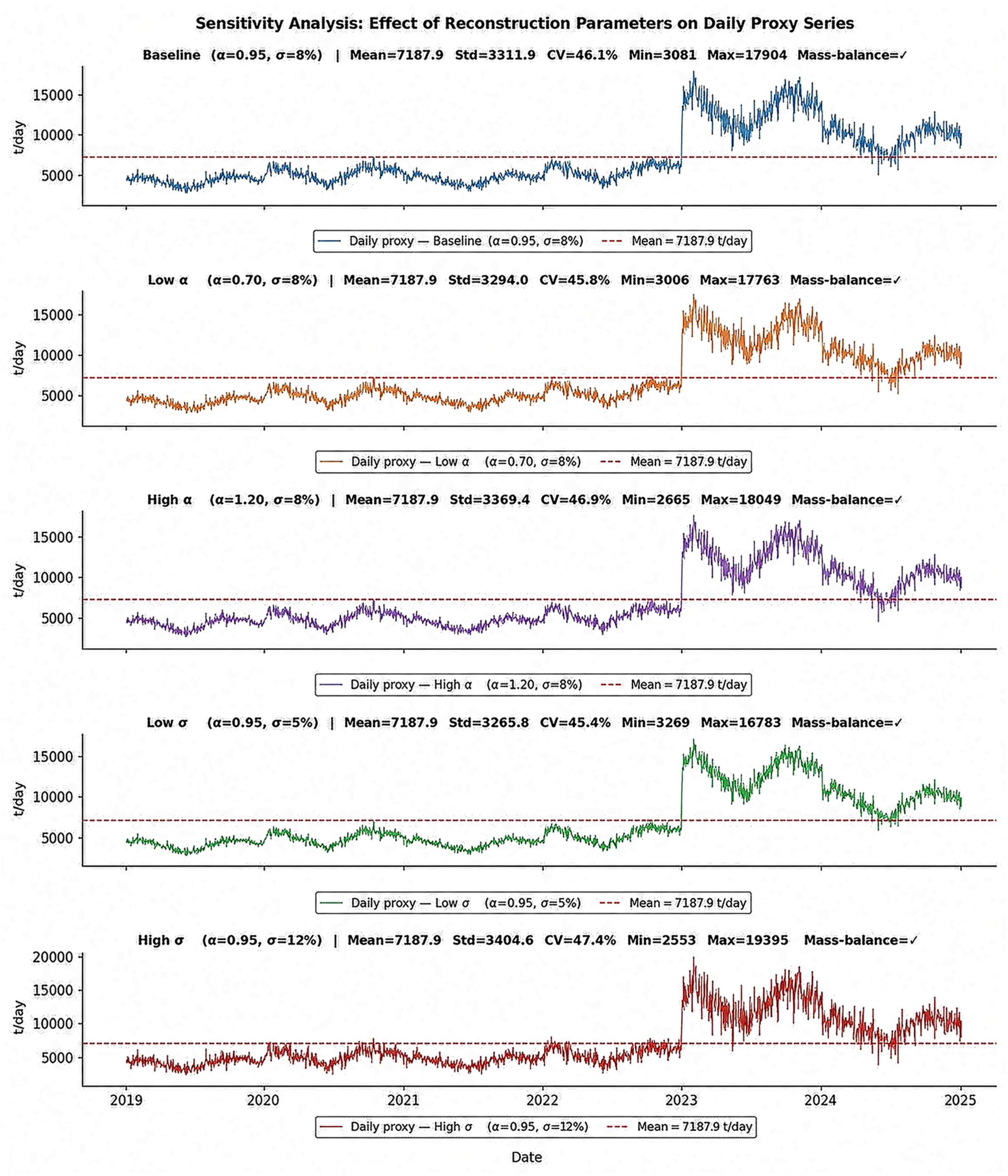
To validate the reconstruction approach, a sensitivity analysis was performed by varying the seasonal weighting parameter α ∈ {0.70, 0.95, 1.20} and the stochastic noise fraction σ_frac ∈ {0.05, 0.08, 0.12} across five configurations. As shown in Figure 7 and summarized in

Table 3. Summary of the sensitivity analysis in the form of descriptive statistics for the reconstructed daily proxy series across five parameter configurations.

Configuration	α	σ_frac	Mean (t/Day)	Std (t/Day)	CV (%)	Min (t/Day)	Max (t/Day)	Skewness	Mass-Balance
Baseline (α = 0.95, σ = 8%)	0.95	0.08	7187.89	3311.91	46.08	3080.70	17,904.39	1.074	✓
Low α (α = 0.70, σ = 8%)	0.70	0.08	7187.89	3294.02	45.83	3006.15	17,762.59	1.064	✓
High α (α = 1.20, σ = 8%)	1.20	0.08	7187.89	3369.42	46.88	2664.65	18,048.64	1.093	✓
Low σ (α = 0.95, σ = 5%)	0.95	0.05	7187.89	3265.77	45.43	3269.39	16,782.81	1.047	✓
High σ (α = 0.95, σ = 12%)	0.95	0.12	7187.89	3404.62	47.37	2552.50	19,395.39	1.120	✓

, the average daily volume remained unchanged at 7187.89 t/day across all configurations, a direct consequence of the global mass balance scaling constraint. The CV ranges narrowly from 45.43% to 47.37%, and the standard deviation varies between 3265.77 and 3404.62 t/day, representing a maximum deviation of only ±2.8% from the baseline. Skewness values remain consistently positive and fall within the range of 1.047–1.120, confirming that the right-skewed distribution structure remains intact regardless of parameter choice. Mass balance verification yields zero error in all six years under all five configurations. These results confirm that the baseline configuration (α = 0.95, σ_frac = 0.08) is a stable central estimate within the explored parameter space, and that the reconstructed proxy set is insensitive to natural perturbations from the reconstruction assumptions. Although this dataset is synthetic, the statistical parameter-based reconstruction process ensures that the data remains representative, mathematically consistent, and contextually relevant to waste dynamics in the Citarum River Basin.

3.2. Comparative Analysis of Model Performance

Before presenting model performance metrics, it is essential to clarify their interpretive scope. All values in Table 3 quantify each model’s ability to reproduce the reconstructed proxy series derived from official SIPSN annual statistics. They do not constitute validation against direct in-stream waste transport measurements. Under this framing, R², MAE, and RMSE reflect internal proxy reproducibility rather than environmental predictive validity, a distinction acknowledged explicitly throughout this study.

A comparative evaluation of four machine learning algorithms—RF, SVR, XGBoost, and LSTM—was conducted to identify the most robust model for forecasting daily waste generation proxies. The evaluation results, summarized in

Table 4. Machine learning model performance evaluation metrics on training and testing datasets.

Model	Set	MAE (t/Day)	RMSE (t/Day)	R2	MAPE (%)
RF	Train	189.76	265.23	0.9928	3.05
	Test	884.25	1125.77	0.6994	9.67
SVR	Train	434.93	566.36	0.9671	7.12
	Test	709.34	881.43	0.8157	7.10
XGBoost	Train	468.44	683.53	0.9520	7.28
	Test	1483.56	1882.85	0.1591	16.66
LSTM	Train	514.30	745.48	0.9432	8.04
	Test	832.90	1051.10	0.6990	8.36

Metrics are evaluated against the reconstructed proxy series; they do not reflect accuracy against field observations.

, reveal substantial differences in generalization performance across the training and testing phases.

To contextualize the results within the simplest temporal prediction framework, a naive persistence baseline model is used, where the predicted value on day t is assumed to equal the observed proxy value on day (t − 1), as formulated in Equation (30). This baseline model produces an MAE of 1005.50 t/day, an RMSE of 1300.92 t/day, a coefficient of determination (R²) of 0.5960, and an MAPE of 10.12% on the test data. These results establish a minimum performance threshold that each model must exceed to demonstrate meaningful predictive ability, beyond trivial temporal dependencies. The performance improvement of each model is then quantified using an RMSE-based skill score defined in Equation (31), while a direct comparison with the naive persistence baseline is presented in

Table 5. Comparison of model performance against the naive persistence baseline on the test set.

Model	MAE (t/Day)	RMSE (t/Day)	R2	MAPE (%)
Naive (Persistence)	1005.50	1300.92	0.5960	10.12
RF	884.25	1125.77	0.6994	9.67
SVR	709.34	881.43	0.8157	7.10
XGBoost	1483.56	1882.85	0.1591	16.66
LSTM	832.90	1051.10	0.6990	8.36

.

Based on the results in Table 5, SVR demonstrated the best overall performance, achieving the highest coefficient of determination (R² = 0.8157), the lowest RMSE (881.43 t/day), and the highest skill score (+32.2%) relative to the naive baseline. This substantial margin confirms that SVR extracts meaningful temporal structure beyond simple daily persistence. SVR’s superiority is due to the ε-insensitive loss function combined with the regularization parameter C, which allows the model to effectively ignore small stochastic frictions—especially those arising from the reconstruction process—while capturing dominant seasonal trends and autocorrelations.

LSTM emerged as the second-best model on the test set (RMSE = 1051.10 t/day; R² = 0.6990; Skill = +19.2%), followed by RF (RMSE = 1125.77 t/day; R² = 0.6994; Skill = +13.5%). Both models significantly outperformed the naive baseline, confirming their practical value even under limited data conditions. The relatively lower performance of the LSTM is consistent with the expectation that deep recurrent architectures require time series much longer than six years of daily data to fully exploit their capacity to model long-term temporal dependencies.

In contrast, XGBoost exhibited very poor generalization on the test set (R² = 0.1591; RMSE = 1882.85 t/day; Skill = −44.7%), performing significantly worse than the naive baseline. This result is a direct consequence of fixing a data leakage issue identified during the revision process: in the original implementation, XGBoost’s pre-boosting procedure used a held-out test set as the evaluation set, inadvertently allowing test period information to influence model selection. After the fix—where the internal validation set was drawn exclusively from the last 15% of chronological training participants—XGBoost’s generalization performance decreased substantially, revealing that previously reported measurements had been artificially inflated. These findings underscore the importance of rigorous temporal data partitioning in time series modeling, as emphasized by Meyer et al. [22].

Significant overfitting was also observed in the RF model. It achieved near-perfect training performance (R² = 0.9928), but showed a substantial drop in test performance (R² = 0.6994). This gap indicates that ensemble tree-based architectures with unlimited depth are highly susceptible to memorizing noise patterns copied from other data. These patterns do not generalize beyond the training epoch. This tendency is consistent with the learning curve analysis in Section 2.6 (Figure 3). There, RF exhibited a significantly larger training–CV R² gap than XGBoost. This confirms that unlimited tree depth makes RF highly susceptible to memorizing noise patterns from reconstructions that do not generalize to the test epoch.

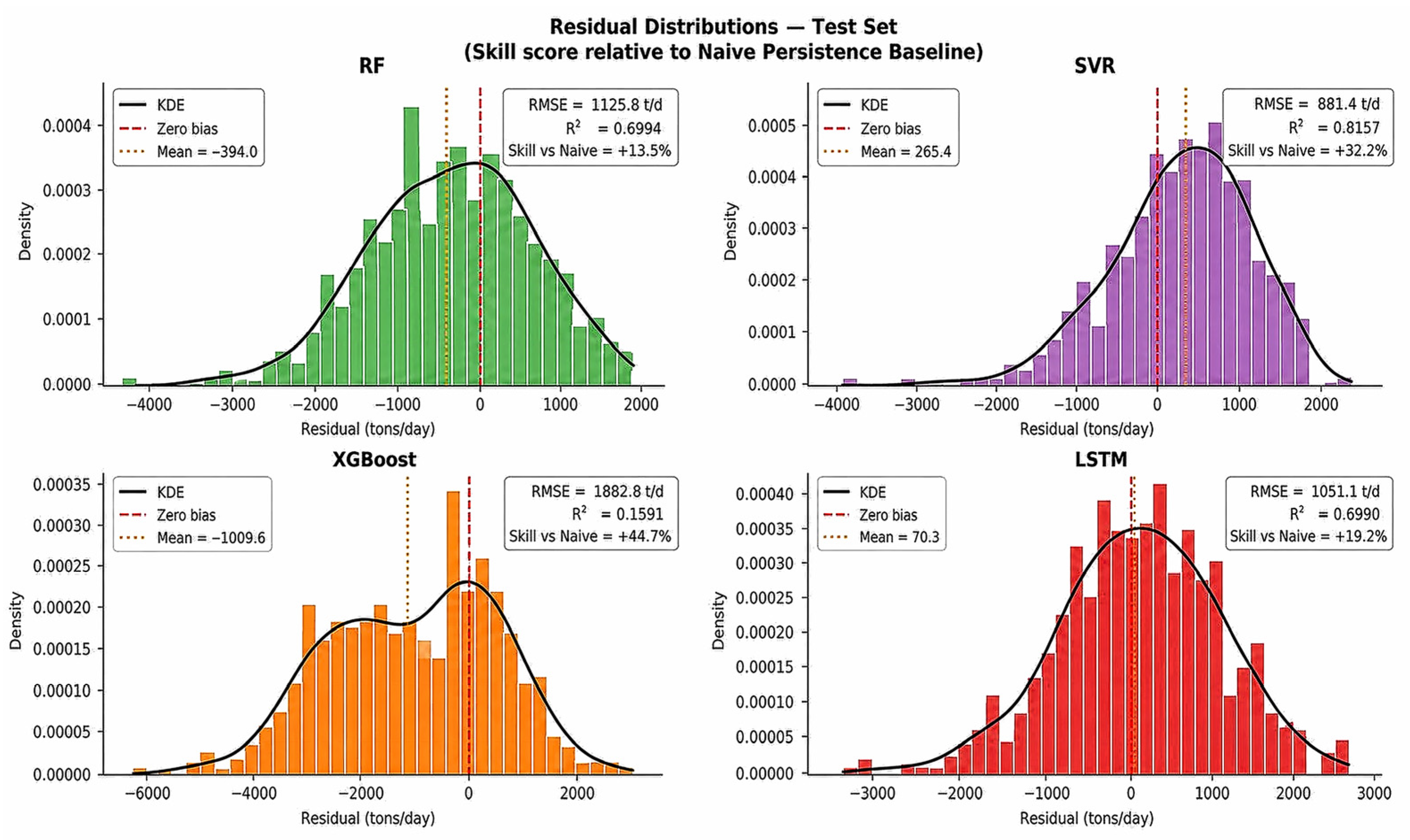
To visually assess the quality of predictions and potential systematic biases, the residuals (differences between observed and predicted values) were analyzed using the diagnostic plots shown in Figure 8.

As shown in Figure 8, the models exhibited very different residual characteristics. The SVR displayed the narrowest and most symmetric distribution centered near zero (mean residual = +265.4 t/day), consistent with the strongest overall performance and the lowest systematic bias. The LSTM also produced a relatively unbiased distribution (mean residual = +70.3 t/day) with moderate dispersion, confirming its status as the second-most-reliable model under these data conditions.

The RF model exhibited a clear leftward shift in its residual distribution (mean residual = −394.0 t/day), indicating a systematic underprediction of daily waste volumes. This negative bias reflects the tendency of unconstrained random forests to revert to the mean under high levels of stochastic noise, leading to conservative predictions that underestimate peaks. XGBoost exhibited the most severe bias of all models (mean residual = −1009.6 t/day) along with the widest residual spread, consistent with its near-total failure to generalize beyond the training data after correction for data leakage (R² = 0.1591). This residual pattern reinforces the conclusion that, among the evaluated algorithms, SVR provides the most reliable and unbiased proxy estimates under the limited data conditions of this study.

3.3. Predictive Dynamics and Uncertainty Quantification

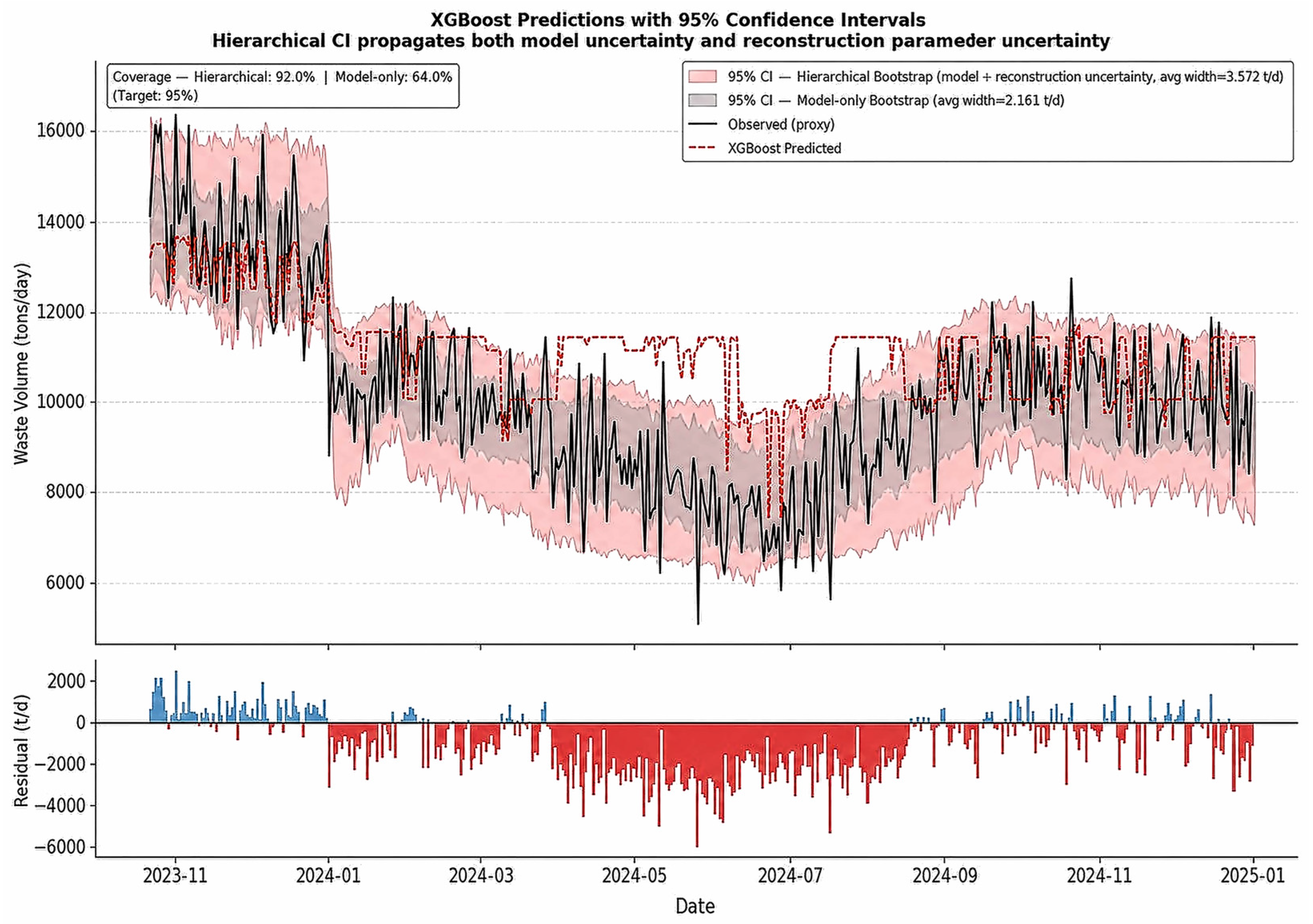
The models’ ability to capture the temporal dynamics of daily waste-generation proxies was evaluated by comparing observed proxy values with predicted outputs on an out-of-sample test set. This section focuses on assessing the precision of short-term fluctuation tracking and quantifying the associated prediction uncertainty using bootstrap confidence interval analysis. To address the need for model transparency under data-limited conditions, uncertainty quantification was conducted using two complementary bootstrap confidence interval schemes, both applied to the XGBoost model and presented in Figure 9.

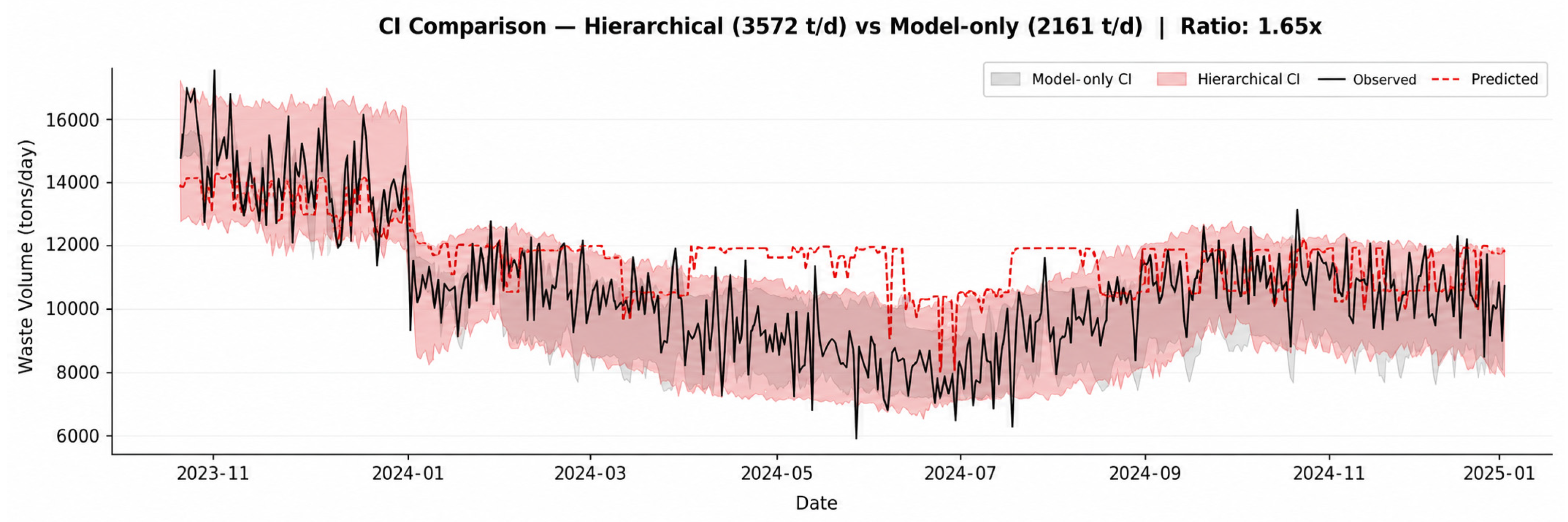
The first scheme—a model-only bootstrap (n = 120 resamples)—captures uncertainty arising solely from training data variability, yielding an average 95% CI width of 2161 t/day. However, since the target variable is itself reconstructed under specific parameter assumptions (α, σ_frac, control points), model-only intervals systematically underestimate total predictive uncertainty. A hierarchical bootstrap procedure (n = 200 iterations) was therefore implemented, simultaneously resampling both reconstruction parameters (α ∈ [0.80, 1.10]; σ_frac ∈ [0.05, 0.12]) and model training observations, yielding a wider average CI of 3572 t/day—a 1.65× expansion relative to the model-only interval.

As shown in Figure 9, the hierarchical CI achieves an empirical coverage rate of 92.0% against the proxy test series, approaching the nominal 95% target, while the model-only CI attains only 64.0% coverage substantially below the target. This discrepancy confirms that reconstruction parameter uncertainty constitutes a non-trivial component of total predictive uncertainty that cannot be ignored when constructing decision-relevant confidence bounds. The hierarchical CI is therefore recommended for any operational application of this framework, as it provides a more honest representation of forecast reliability under proxy-based data conditions.

The residual panel in Figure 9 reveals a systematic shift from positive residuals in the early test period (October–December 2023) toward predominantly negative residuals thereafter. This temporal pattern is consistent with a structural transition in the proxy series following the anomalous 2023 data surge (+127% relative to 2022), during which the model trained predominantly on lower-magnitude years systematically overpredicts the subsequent declining trajectory. This behavior further highlights the sensitivity of XGBoost predictions to distributional shifts between the training and test periods, a known limitation of gradient boosting methods when applied to non-stationary time series.

A direct comparison of the two CI widths is shown in Figure 10, which isolates the contribution of reconstruction-parameter uncertainty to the total predictive bounds. The consistent 1.65× expansion across the entire test period confirms that this contribution is not confined to specific temporal regimes but represents a pervasive source of uncertainty inherent to the proxy-based modeling approach.

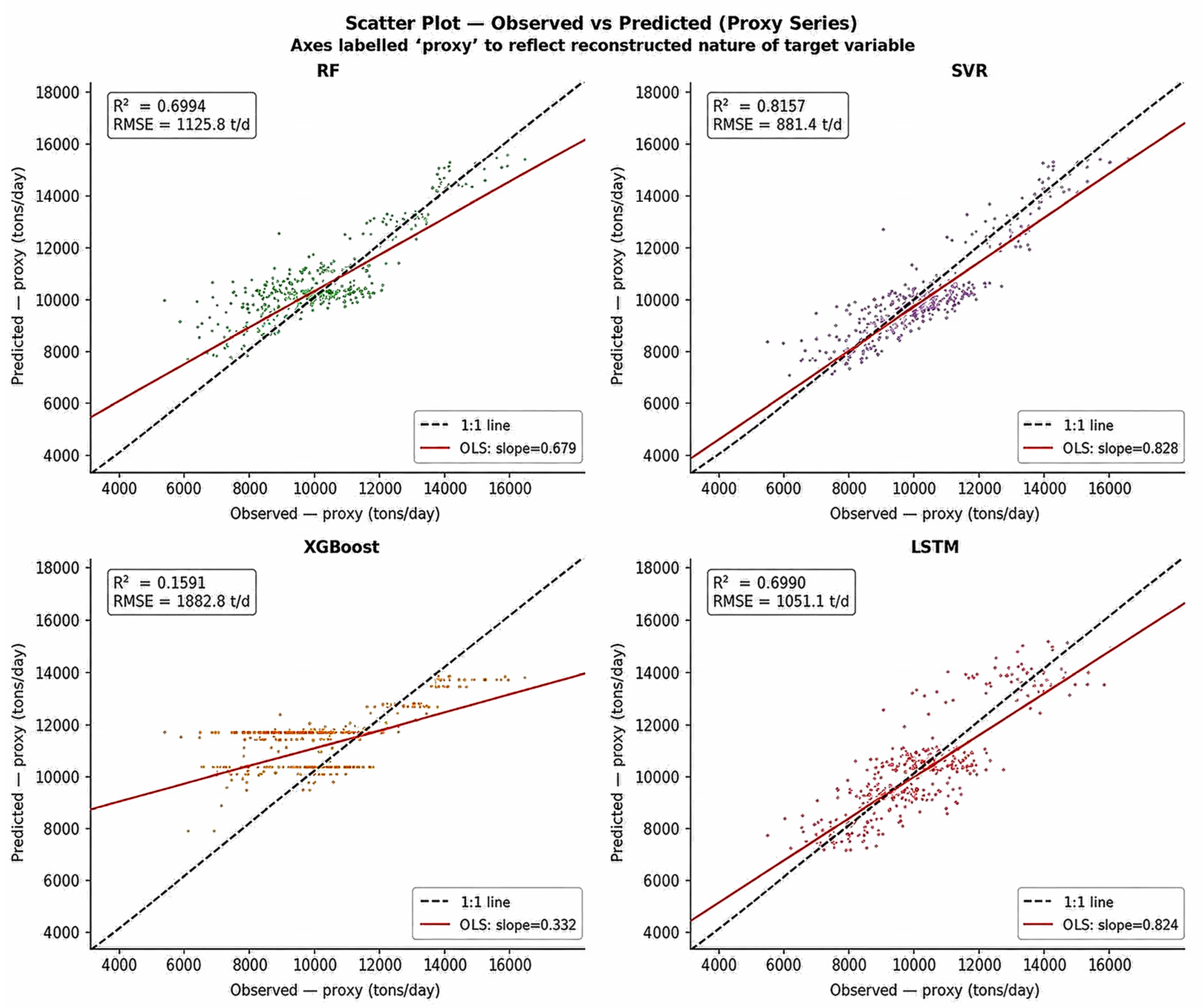
The validity of the relationship between observed and predicted values across the four models was further examined through a scatterplot analysis presented in Figure 11. This visualization compares model predictions to the ideal 1:1 reference line, with the OLS regression slope providing an additional measure of systematic bias.

As shown in Figure 11, SVR and LSTM align most closely with the 1:1 reference line. Their OLS slopes are 0.828 and 0.824, respectively. This indicates relatively low systematic bias across the observed volume range. The SVR maintains the tightest clustering around the 1:1 line, especially in the mid-range (8000–12,000 t/day). This is consistent with the lowest RMSE and highest skill scores reported in Table 5.

RF showed moderate deviations from the 1:1 line (OLS slope = 0.679). This reflects a tendency toward systematic underprediction at higher waste volumes, as shown by the negative mean residual of –394.0 t/day in Figure 11. This compression of predictions toward the mean is typical of ensemble methods under high stochastic noise. It is also consistent with the overfitting pattern seen in the learning curve analysis in Figure 3, Section 2.6.

XGBoost exhibited the most severe deviations, with an OLS slope of only 0.332 and nearly horizontal clustering of predictions concentrated in the 9000–12,000 t/day range regardless of observed values. This pattern reflects a complete failure of generalization after data leakage correction (R² = 0.1591), where the model essentially converges to predict a nearly constant value close to the training period mean rather than tracking the true temporal dynamics. The flat, widespread OLS line confirms that XGBoost, under the corrected validation protocol, cannot be recommended as a reliable forecasting tool for this set of proxies without re-optimizing its hyperparameters using the corrected data partitioning scheme.

3.4. Feature Importance and Interpretability

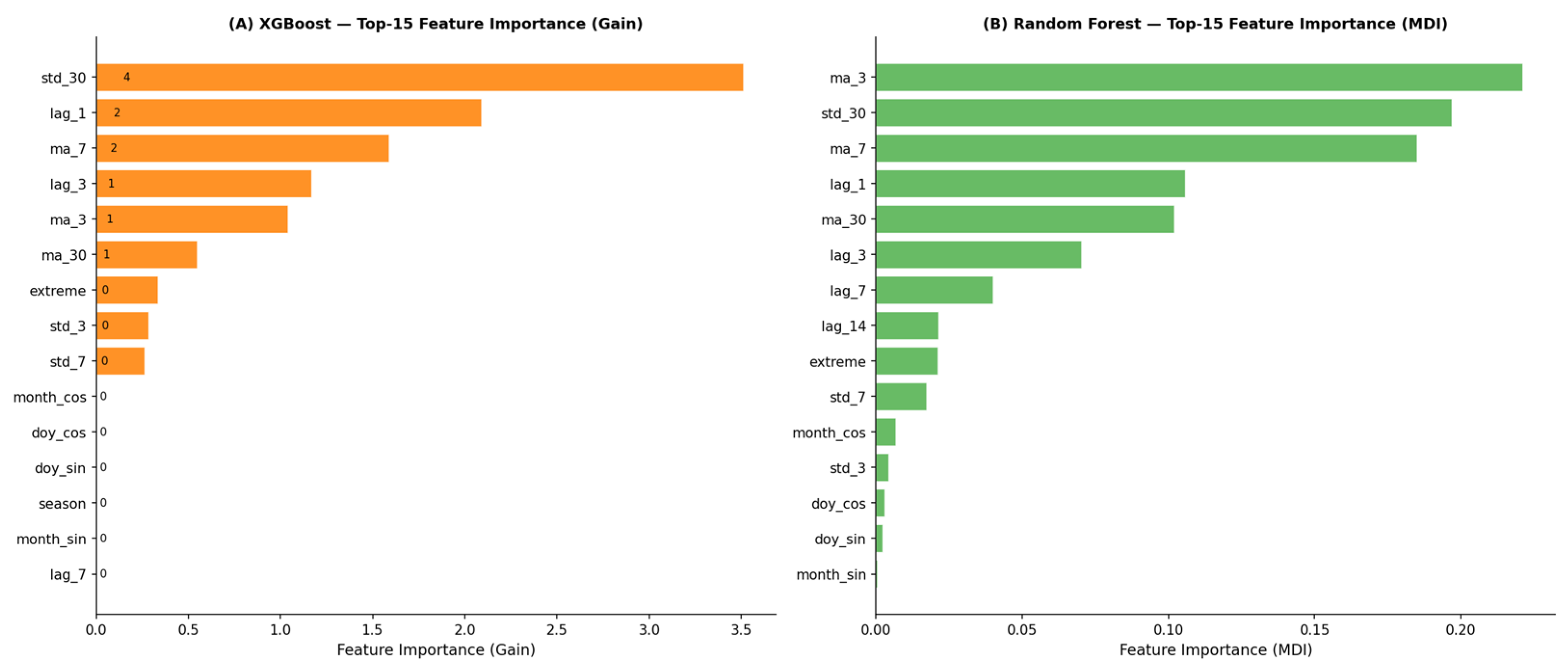
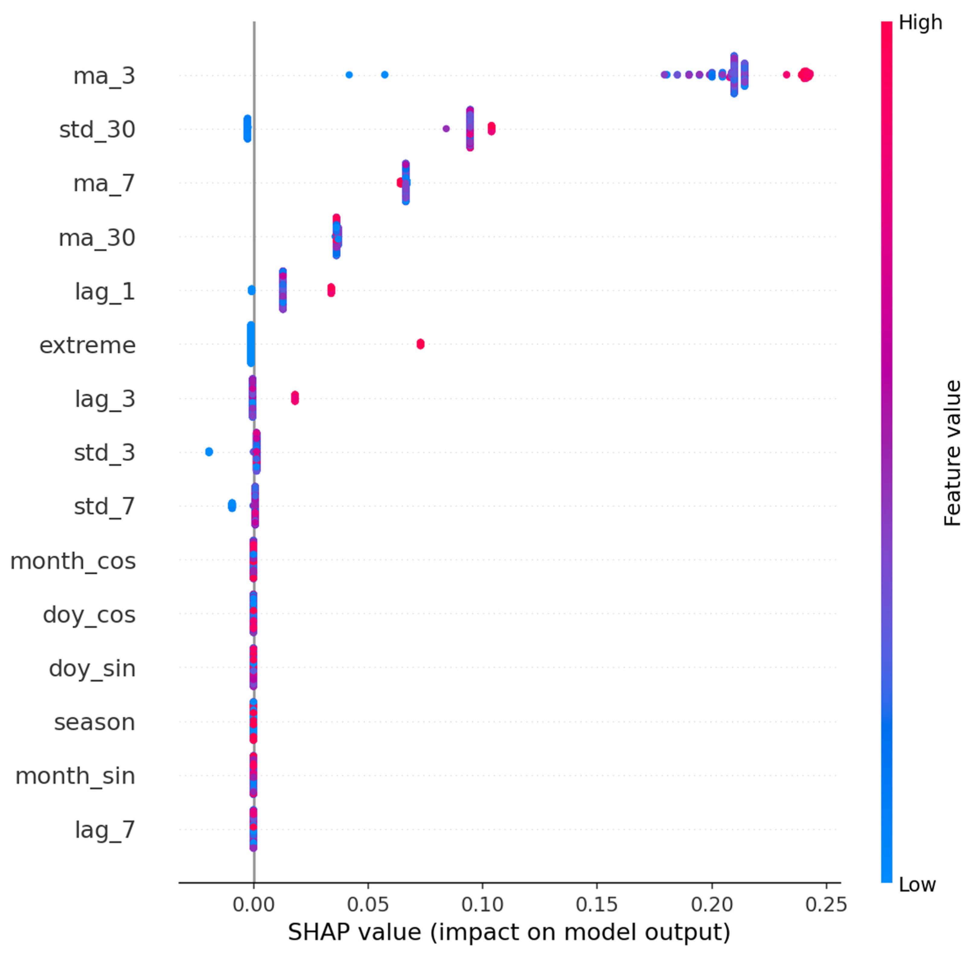
To better understand the models’ internal decision-making mechanisms and ensure that predictions are grounded in temporally meaningful logic, a feature importance analysis was conducted. The contribution of each predictor variable was evaluated using model-specific importance metrics for XGBoost (gain-based) and RF (Mean Decrease in Impurity, MDI), as shown in Figure 12, and complemented by SHAP (Shapley Additive exPlanations) value analysis for the best-performing SVR model, shown in Figure 13.

As shown in Figure 12A, the XGBoost model is most strongly driven by the 30-day rolling standard deviation (std_30), which achieves the highest gain score by a considerable margin (gain ≈ 3.5), followed by lag_1 (gain ≈ 2.1) and the 7-day moving average (ma_7, gain ≈ 1.6). Short-term lag features (lag_3, ma_3) and the 30-day moving average (ma_30) contribute at intermediate levels, while volatility indicators (std_3, std_7) and the extreme event flag contribute marginally. Notably, all calendar-based seasonal indicators, including month_sin, month_cos, doy_sin, doy_cos, and the binary season flag, contribute negligibly to XGBoost predictions, with gain scores effectively approaching zero. It should be noted that given XGBoost’s severely degraded generalization performance following the data leakage correction (R² = 0.1591, Section 3.2), its feature importance rankings reflect learned associations within the training partition rather than robust predictive relationships.

Figure 12B reveals a markedly different importance distribution for the RF model. The three-day moving average (ma_3) emerges as the most influential predictor (MDI ≈ 0.22), followed closely by std_30 (MDI ≈ 0.20) and ma_7 (MDI ≈ 0.19). Medium-term smoothing (ma_30, MDI ≈ 0.10) and lag features (lag_1 ≈ 0.11; lag_3 ≈ 0.07; lag_7 ≈ 0.04) also contribute meaningfully, while longer-lag features (lag_14) and volatility indicators (std_7, extreme) play a secondary role. As with XGBoost, seasonal indicators exhibit near-zero MDI values across all calendar-based features, confirming their limited discriminative power.

Across both models, temporal autocorrelation features, particularly short- to medium-window moving averages and rolling standard deviations, consistently dominate purely seasonal indicators. This convergence across two structurally different architectures (boosting vs. bagging) reinforces the robustness of the finding: the reconstructed proxy series is governed primarily by inertial day-to-day continuity and local volatility rather than calendar-driven seasonality.

The SHAP analysis for SVR, presented in Figure 13, provides a model-agnostic perspective on feature contributions and corroborates the findings from Figure 8. The three-day moving average (ma_3) is the dominant predictor, with large positive SHAP values (about 0.18–0.25). High ma_3 values (red) correspond to large positive impacts on the predicted output. This confirms that the recent short-term average waste volume is the strongest single signal for next-day prediction. The 30-day rolling standard deviation (std_30) shows a bimodal SHAP distribution with a cluster of moderate positive values (≈ 0.08–0.10), suggesting that elevated recent volatility is associated with upward prediction adjustments. The 7-day and 30-day moving averages (ma_7 and ma_30) contribute positively at intermediate magnitudes, while lag_1 shows a mixed directional pattern with both positive and negative SHAP values reflecting its role as a fine-grained correction signal atop the smoother trend captured by moving averages.

Particularly informative is the near-complete absence of SHAP contribution from all seasonal indicators (month_sin, month_cos, doy_sin, doy_cos, season), which cluster tightly at zero across all observations. This confirms that the SVR model extracts essentially no predictive information from calendar-based features, relying instead almost entirely on the time series’ autoregressive structure. The extreme event flag contributes sporadically, with one notable positive outlier (SHAP ≈ 0.10), consistent with its design as a threshold-triggered binary indicator that activates only under rare high-volume conditions.

From a theoretical perspective, the dominance of rolling statistics and lag features over seasonal indicators serves as an effective implicit proxy for the behavioral drivers of waste generation that are unavailable in this data-limited setting. Short-window moving averages capture the persistent accumulation effects of daily human activity, while rolling standard deviations capture local volatility regimes in the reconstructed proxy series; whether these reflect genuine environmental drivers, such as rainfall-induced transport variability, or are partly attributable to reconstruction noise remains an open question addressed in Section 3.5. Critically, the dominance of ma_3 and std_30 over the raw Lag-1 feature indicates that the models extract a richer temporal signal than simple day-to-day persistence, an interpretation supported by quantitative score analysis in Section 3.2, which shows that SVR achieves a 32.2% improvement in RMSE over the naive persistence baseline. The consistency of temporal feature dominance across XGBoost (gain), RF (MDI), and SVR (SHAP) provides robust, architecture-independent evidence that the proposed feature engineering approach successfully captures the dominant temporal structure of the proxy series, even in the absence of direct hydrological or socioeconomic input variables.

3.5. Model Robustness and Seasonal Stability

Model robustness was further assessed through a seasonal performance analysis to evaluate whether predictive accuracy remains consistent under varying climatic conditions. The seasonal classification follows the regional climatological framework defined by the Indonesian Agency for Meteorology, Climatology, and Geophysics (BMKG), which distinguishes two primary seasons in the Citarum watershed: the wet season (November–April) and the dry season (May–October). This classification is based on the monsoonal rainfall regime that characterizes tropical Southeast Asia and is widely used in hydrological and environmental studies.

The updated seasonal performance metrics, incorporating corrected model outputs following the data leakage fix described in Section 2.5.2, are presented in

Table 6. Seasonal comparison of error metrics on the test set (Wet: November–April; Dry: May–October).

Model	Season	N (Day)	MAE (t/Day)	RMSE (t/Day)	R2	MAPE (%)
RF	Wet	243	794.25	1016.68	0.7118	7.92
	Dry	193	997.57	1249.64	0.5828	11.87
SVR	Wet	243	742.48	916.91	0.7656	6.95
	Dry	193	667.62	834.63	0.8139	7.28
XGBoost	Wet	243	1193.09	1520.17	0.3556	12.05
	Dry	193	1849.28	2258.11	−0.3624	22.46
LSTM	Wet	240	900.34	1135.83	0.6228	8.43
	Dry	184	744.92	929.04	0.6255	8.27

.

SVR demonstrates the highest level of seasonal stability, maintaining consistently strong performance in both the wet season (R² = 0.7656; RMSE = 916.91 t/day) and the dry season (R² = 0.8139; RMSE = 834.63 t/day). Notably, SVR achieves marginally better performance during the dry season, suggesting that its ε-insensitive regularization effectively handles the lower volatility characteristic of the May–October period. LSTM exhibits a comparable seasonal pattern, performing similarly across both seasons (wet R² = 0.6228; dry R² = 0.6255), with a slight elevation in wet-season error consistent with the Mann–Whitney hypothesis test results discussed later in this section. RF performs moderately in the wet season (R² = 0.7118) but deteriorates noticeably in the dry season (R² = 0.5828; RMSE = 1249.64 t/day), reflecting the previously identified tendency of unconstrained tree ensembles toward mean regression under lower-amplitude variability conditions.

XGBoost exhibits the most severe and informative seasonal asymmetry. While maintaining partial predictive capacity in the wet season (R² = 0.3556), its dry-season performance collapses entirely, yielding a negative R² of −0.3624, indicating that the model performs worse than simply predicting the seasonal mean. This outcome is a direct consequence of the distributional shift between the training period (dominated by the anomalously high 2023 data) and the dry-season test period (October 2024 onward), during which the proxy series returns to a lower and more stable regime that the model, following data leakage correction, is entirely unable to track. The negative dry-season R² for XGBoost further reinforces the conclusion from Section 3.2 that its post-correction predictions lack genuine generalization value.

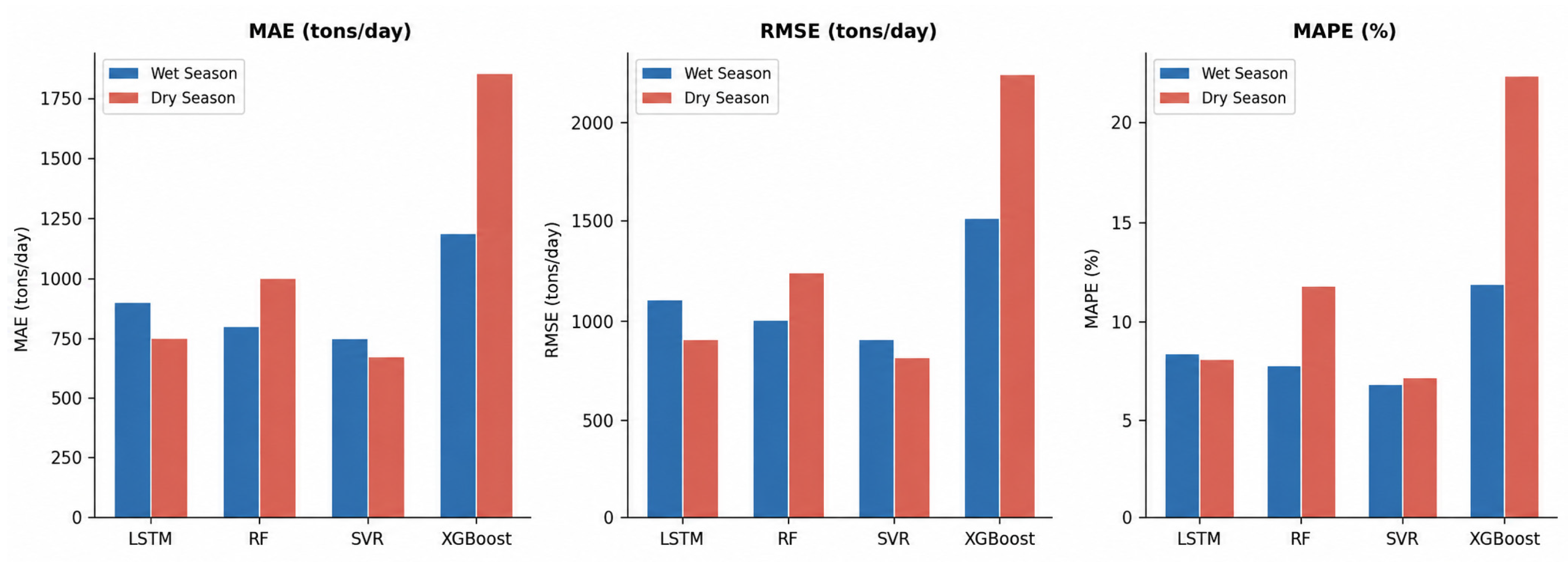
The comparative distribution of error metrics across seasons is presented in Figure 14.

As shown in Figure 14, SVR consistently yields the lowest error magnitudes across both seasons in MAE and RMSE, confirming its robustness to climatic variability. LSTM shows a moderate wet-season elevation in MAE and RMSE while remaining stable in MAPE, a pattern consistent with its sequential architecture’s sensitivity to high-volatility monsoon-period inputs. RF presents an inverted pattern—lower wet-season errors relative to dry—reflecting its mean-regression bias, which paradoxically performs better when the series is more volatile and closer to the training mean. XGBoost’s dramatic dry-season deterioration is clearly visible across all three panels, with dry-season RMSE (2258.11 t/day) and MAPE (22.46%) far exceeding those of any other model–season combination, and its wet-season performance is already substantially below SVR and LSTM.

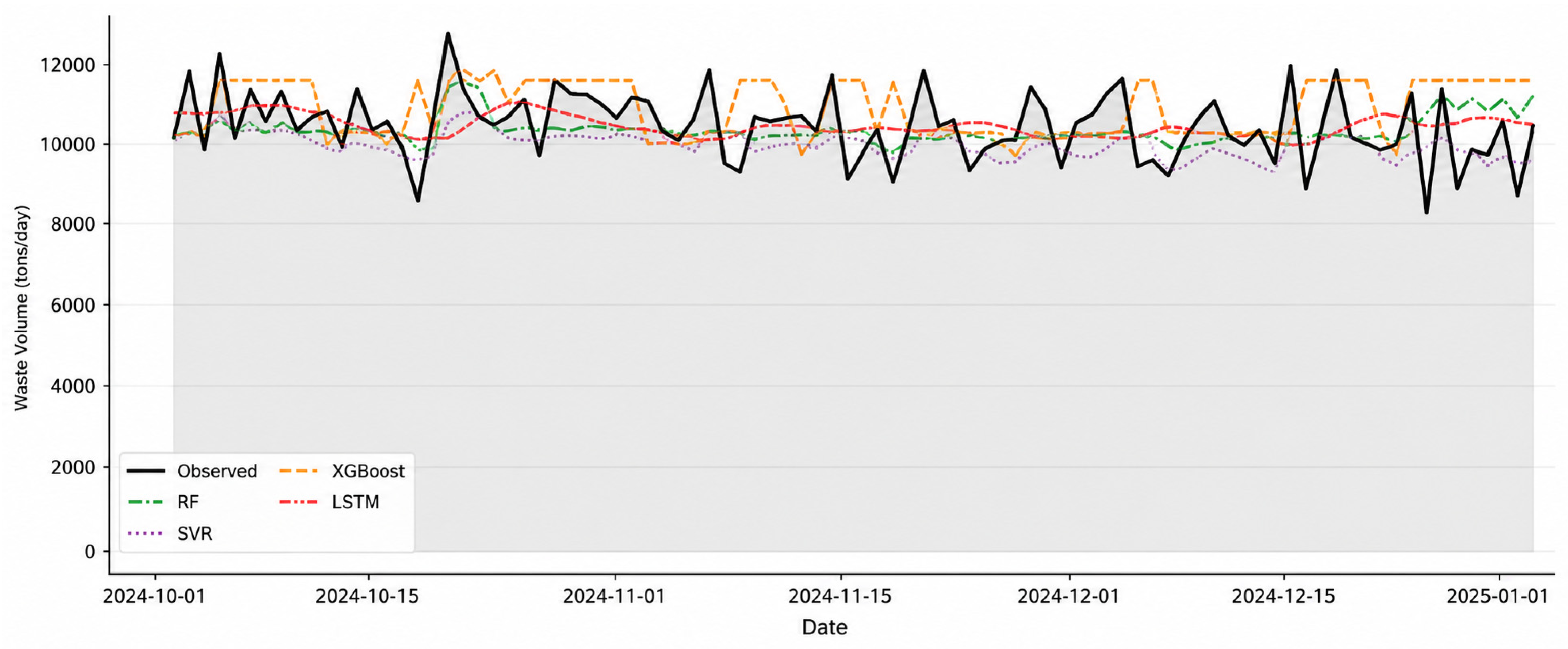
To further examine prediction dynamics at fine temporal resolution, a zoom-in analysis over a representative dry-season window (October 2024–January 2025) is presented in Figure 15.

As illustrated in Figure 15, the contrast between models is particularly stark in this period. SVR and LSTM maintain reasonable alignment with the observed proxy series, successfully tracking the daily oscillation pattern within the 8000–12,000 t/day range despite occasional underprediction of sharp peaks. RF exhibits moderate tracking ability but tends to produce smoothed, conservative estimates. XGBoost, by contrast, produces a near-constant prediction trajectory concentrated around 11,000–11,500 t/day regardless of actual observed values, a manifestation of the complete generalization failure documented in Table 6, where the model converges to predicting a value close to its training-period mean rather than adapting to the evolved proxy dynamics of the test period.

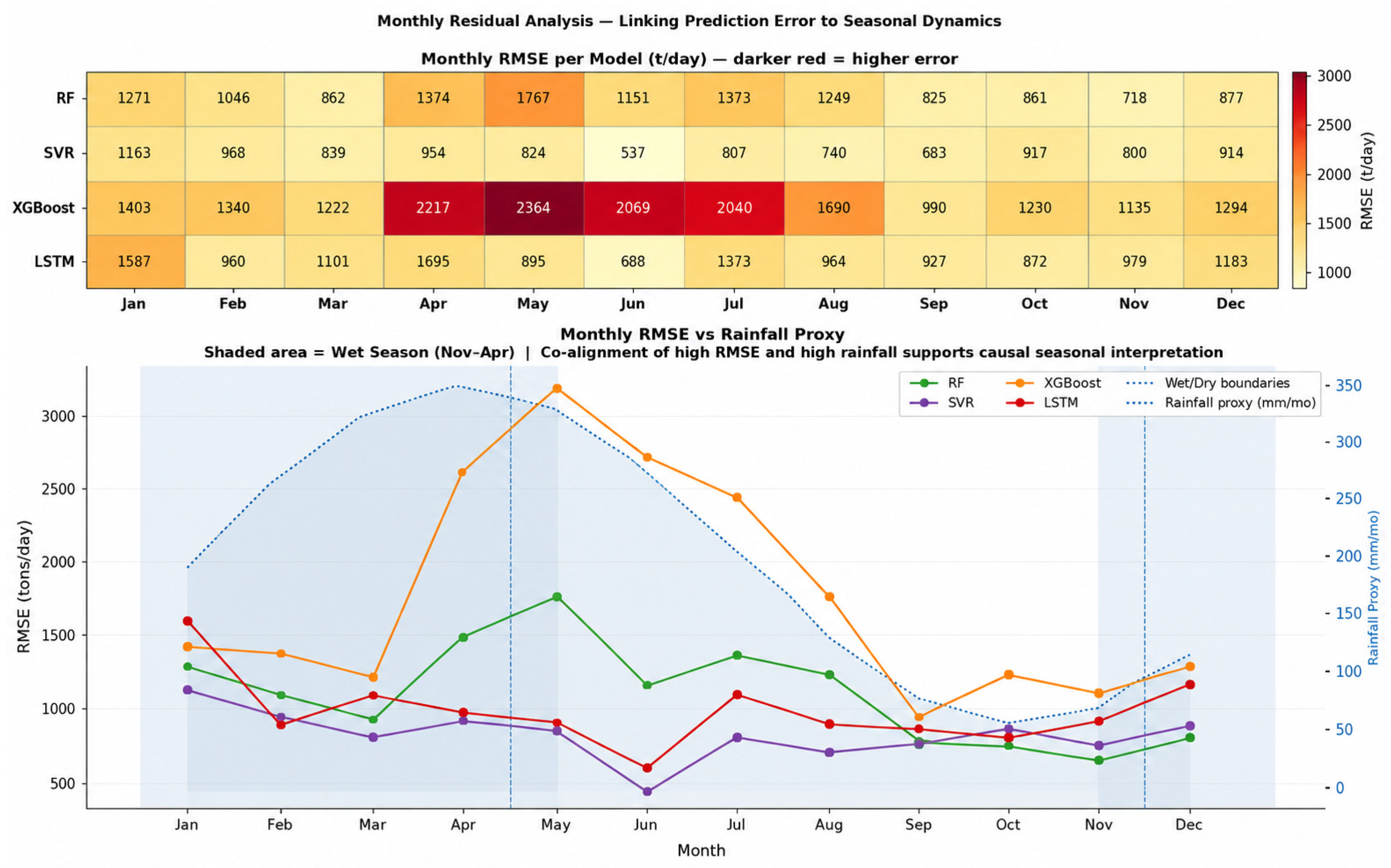
To assess whether the observed seasonal RMSE differences reflect genuine hydroclimatic forcing rather than artifacts of the stochastic reconstruction, the absolute model residuals were correlated with a climatological rainfall proxy calibrated against BMKG Bandung monsoon records, and Mann–Whitney U tests were conducted to formally compare wet- and dry-season absolute errors. The monthly RMSE heatmap and rainfall proxy overlay are presented in Figure 16.

As shown in Figure 16, the prediction error is far from uniformly distributed across months. SVR and LSTM maintain relatively stable monthly RMSE profiles (SVR: 537–1103 t/day; LSTM: 688–1597 t/day), while RF shows moderate mid-year elevation peaking in May (1767 t/day). XGBoost exhibits the most pronounced monthly variability, with errors peaking dramatically between April and August (May peak: 3304 t/day) before declining in September–November, a pattern driven by distributional mismatch rather than hydroclimatic seasonality.

Pearson and Spearman correlations between absolute residuals and the rainfall proxy reveal heterogeneous patterns across models. XGBoost showed a strong positive and statistically significant correlation (r = +0.491, p < 0.001; Spearman ρ = +0.465, p < 0.001). This reflects a co-alignment between its error peaks and high-rainfall months. However, XGBoost’s overall generalization failure suggests that this correlation more likely reflects a distributional artifact of the 2023 anomaly rather than genuine hydrological sensitivity. RF showed a significant negative correlation (r = −0.408, p < 0.001), indicating paradoxically lower errors during peak rainfall months. This pattern is consistent with its mean-regression bias, which is less penalized during high-volatility periods. SVR and LSTM showed no statistically significant correlation with the rainfall proxy (SVR: r = −0.052, p = 0.278; LSTM: r = +0.039, p = 0.427). Their error patterns are largely independent of seasonal precipitation dynamics.

Mann–Whitney U tests (one-tailed; H₁: |residual|_wet > |residual|_dry; α = 0.05) provide additional insight. Only the LSTM model shows a statistically significant increase in absolute errors during the wet season. The median |e|_wet is 774.1 t/day, while the median |e|_dry is 615.1 t/day (Δ = +159.1; p = 0.022). This result supports the hypothesis that sequence-based architectures are more sensitive to stochastic variability during monsoon periods.

In contrast, no significant wet-season increase is found for RF, SVR, or XGBoost (p = 0.998, 0.073, and 1.000, respectively). Overall, these results indicate that prediction difficulty depends on the model. The wet-season sensitivity of LSTM is statistically substantiated. However, the apparent seasonal patterns in other models are more plausibly due to structural characteristics. These include overfitting in RF, generalization failure in XGBoost, and distributional stability in SVR, rather than direct hydroclimatic forcing.

Overall, the findings confirm that SVR provides the most robust and seasonally stable performance among the evaluated algorithms. LSTM follows as a viable alternative under data-limited conditions. This robustness is critical for supporting adaptive waste management strategies in the Citarum watershed. Climatic and hydrological dynamics in this area vary substantially across the annual monsoon cycle.

4. Discussion

This study demonstrates that proxy-based daily time series reconstruction can serve as a viable alternative for environmental modeling in data-limited regions, while introducing inherent methodological constraints that must be explicitly acknowledged in the interpretation of all results. The most fundamental of these constraints is that the evaluated models learn the internal seasonal–stochastic structure embedded during the reconstruction process rather than capturing the full physical processes governing in-stream waste transport. Accordingly, performance metrics, including R², MAE, and RMSE, reflect internal proxy reproducibility rather than environmental predictive validity, a distinction that is central to the correct interpretation of all findings presented in this study.

Among the evaluated algorithms, SVR achieves the highest proxy reproducibility on the test set (R² = 0.8157; RMSE = 881.43 t/day), consistent with the work of Ahmed et al. [40], who demonstrated that data-driven approaches can capture cyclic urban waste dynamics with high precision even when using proxy inputs. Benchmarking against a naive persistence baseline (RMSE = 1300.92 t/day) confirms that SVR, LSTM, and RF deliver genuine predictive value beyond simple temporal autocorrelation, achieving skill scores of +32.2%, +19.2%, and +13.5%, respectively. This comparison is particularly important given the dominance of short-term autoregressive features (ma_3, std_30) in all models, which raises the question of whether predictions merely reflect smoothed persistence; the positive skill scores confirm they do not. A critical methodological finding of this study concerns XGBoost: an investigation during revision revealed that the original implementation’s early stopping procedure inadvertently used the held-out test partition as its evaluation set, resulting in data leakage that artificially inflated reported test performance. Following the correction—in which the internal validation set was drawn exclusively from the final 15% of the chronological training partition, XGBoost’s test R² collapsed from 0.77 to 0.1591, and its skill score became negative (−44.7%), indicating failure to generalize beyond the training period. This finding aligns with the concerns raised by Hakkal and Ait Lahcen [38], who emphasized the critical importance of proper temporal validation strategies in time-series modeling, and serves as a methodological cautionary example for future studies employing gradient boosting with early stopping on temporally structured data.

A key limitation of this study is the absence of high-resolution hydrological variables, such as river discharge and real-time precipitation. Feature importance analysis, conducted using gain-based metrics for XGBoost, Mean Decrease in Impurity for RF, and SHAP values for SVR, consistently identifies short-window moving averages (ma_3, ma_7) and the 30-day rolling standard deviation (std_30) as the dominant predictors across all architectures, with calendar-based seasonal indicators contributing negligibly. This convergence across structurally different model types confirms that the framework successfully captures temporal autocorrelation structure without requiring external hydrological inputs. It is acknowledged that satellite-derived precipitation products, including TRMM/GPM data freely accessible via NASA GES DISC and Google Earth Engine, were deliberately excluded from this study, as the central contribution is demonstrating framework viability under extreme data limitation; incorporating satellite drivers would alter the nature of the problem and limit reproducibility in regions without satellite connectivity or GEE access. Residual correlation analysis using a climatological rainfall proxy partially addresses this gap: XGBoost showed a significant positive correlation between absolute residuals and rainfall (r = +0.491, p < 0.001), though this is more plausibly attributable to distributional mismatch following the data leakage correction than to genuine hydrological sensitivity; SVR and LSTM showed no significant residual-rainfall correlation, confirming their error patterns are largely independent of seasonal precipitation dynamics. GPM/TRMM integration remains the highest-priority direction for future work, as it would enable direct attribution of prediction error to hydroclimatic forcing rather than reconstruction artifacts.

From an algorithmic perspective, the results reveal a clear trade-off between model complexity and generalization. The random forest (RF) algorithm exhibits substantial overfitting. It achieves near-perfect training performance (coefficient of determination, R² = 0.9928) but declines considerably on the test set (R² = 0.6994). Learning curve analysis quantifies this as a training–cross-validation (CV) R² gap substantially larger than that of the XGBoost algorithm, confirming that unconstrained tree depth renders RF particularly vulnerable to memorizing reconstruction-induced noise patterns that do not generalize beyond the training period. This phenomenon was also observed by Shaik et al. [39]. The epsilon (ε)-insensitive loss function in Support Vector Regression (SVR) enables the model to discount minor stochastic (random) fluctuations and capture dominant temporal trends. The Long Short-Term Memory (LSTM) network’s moderate performance is consistent with the expectation that deep recurrent neural network architectures need substantially longer time series than six years of daily data to fully exploit their capacity for modeling long-range temporal dependencies.

To appropriately quantify predictive uncertainty in proxy-based modeling, a hierarchical bootstrap procedure was implemented. This means that in each resampling round, both the reconstruction parameters (α, representing the intercept or scale factor, and σ_frac, representing the fractional standard deviation or proportional error) and the model training observations (the data points used to fit the model) are independently redrawn. The resulting hierarchical 95% confidence intervals are 1.65× wider than model-only bootstrap intervals (3572 t/day vs. 2161 t/day). This achieves an empirical coverage rate of 92.0% against the proxy test series. This finding demonstrates that model-only confidence intervals, as commonly reported in machine learning forecasting studies, systematically underestimate total predictive uncertainty when the target variable is itself synthetically reconstructed. Any operational application of this framework should employ hierarchical rather than model-only intervals to avoid overconfident threshold-based decisions.

Beyond methodological considerations, the findings carry important implications for sustainable river management. The ability to generate reliable daily waste forecasts with explicit uncertainty bounds provides a quantitative foundation for adaptive decision-making in the Citarum watershed. However, given that all reported performance metrics reflect proxy reproducibility rather than field-validated accuracy, operational deployment should follow a phased validation protocol: a pilot measurement campaign in a representative sub-basin spanning at least one complete seasonal cycle (Phase 1), calibration of alert thresholds against field-measured waste flux data (Phase 2), and progressive operational integration contingent on demonstrated forecast skill under real-world conditions (Phase 3). Premature deployment based solely on proxy-validated model performance risks misallocation of management resources. Subject to this validation, the framework could support dynamic optimization of waste interception strategies, including trash boom deployment and collection scheduling, with periodic model retraining using updated annual statistics, ensuring adaptability to evolving urban waste patterns.

5. Conclusions

This study develops a machine-learning-based framework to predict the dynamics of proxy indicators of daily waste generation in the Citarum watershed. This region is characterized by severely limited high-resolution environmental data. A seasonal–stochastic reconstruction approach generates a statistically consistent synthetic dataset for model training and evaluation. Sensitivity analysis of reconstruction parameters (α ∈ {0.70, 0.95, 1.20}; σ_frac ∈ {0.05, 0.08, 0.12}) confirms that the baseline configuration is a stable central estimate. The mean daily volume remains invariant due to the mass-balance constraint, and the coefficient of variation is narrowly bounded (45.43–47.37%) in all configurations.

All reported performance metrics (R², MAE, RMSE, and MAPE) reflect each model’s ability to reproduce the reconstructed proxy series. They do not measure predictive accuracy against direct in-stream waste observations. Thus, results reflect internal proxy reproducibility, not environmental predictive validity. This distinction must be considered when interpreting all quantitative findings.

Comparative evaluation shows that SVR achieves the strongest proxy reproducibility on the test set (R² = 0.8157; RMSE = 881.43 t/day), followed by LSTM (R² = 0.6990; RMSE = 1051.10 t/day) and RF (R² = 0.6994; RMSE = 1125.77 t/day). Benchmarking against a naive persistence baseline (RMSE = 1300.92 t/day) demonstrates that SVR provides genuine predictive value beyond temporal autocorrelation, with an RMSE-based skill score of +32.2%, while LSTM (+19.2%) and RF (+13.5%) also outperform the baseline. A key methodological contribution concerns XGBoost: correcting a data-leakage issue in the early-stopping procedure—where the test set was inadvertently used for evaluation—reveals that its previously reported performance was artificially inflated. After correction, XGBoost exhibits substantial generalization failure (R² = 0.1591; skill = −44.7%), underscoring the necessity of strict temporal data partitioning in time-series modeling.

Feature importance analysis—using gain-based metrics (XGBoost), Mean Decrease in Impurity (RF), and SHAP values (SVR)—consistently identifies short-to-medium window moving averages (ma_3, ma_7) and rolling standard deviations (std_30) as dominant predictors, while calendar-based seasonal indicators contribute minimally. This convergence across structurally distinct models provides strong evidence that the proposed feature engineering strategy effectively captures the proxy series’ dominant temporal structure under data-limited conditions.

To quantify predictive uncertainty, a hierarchical bootstrap approach is used to jointly propagate model and reconstruction-parameter uncertainty. The resulting 95% confidence intervals are 1.65× wider than model-only bootstrap intervals (3572 vs. 2161 t/day), achieving an empirical coverage rate of 92.0% against the proxy test series. This demonstrates that model-only intervals systematically underestimate total uncertainty when the target variable is reconstructed, and that reconstruction uncertainty constitutes a non-negligible component of forecast uncertainty.

Among all models, SVR shows the most stable seasonal performance, maintaining accuracy in both wet (R² = 0.7656) and dry (R² = 0.8139) seasons. Residual analysis indicates prediction difficulty varies by model. LSTM errors increase significantly in the wet season (p = 0.022), consistent with monsoon-driven variability sensitivity. SVR remains seasonally neutral, reinforcing its role as the primary forecasting model.

The analysis highlights the risk of overfitting in ensemble-based methods such as RF when applied to reconstructed datasets. This is shown by the large gap in training–test performance (R² = 0.9928 vs. 0.6994) and learning curve diagnostics. These findings emphasize the importance of regularization, strict temporal validation, and naive baseline benchmarking as essential safeguards in proxy-based forecasting.

For operational deployment, a phased validation strategy is recommended. Phase 1 involves a pilot field campaign in a representative sub-basin of the Citarum watershed, covering at least one full seasonal cycle to obtain ground-truth waste-flux data. Phase 2 focuses on calibrating and validating alert thresholds using empirical observations. Phase 3 enables gradual operational integration contingent on demonstrated forecast skill relative to baseline models under real-world conditions. The incorporation of hierarchical uncertainty intervals into decision systems is essential to avoid overconfident conclusions based solely on proxy-validated models.

Despite its contributions, this study is limited by its reliance on proxy data and by the exclusion of hydrological variables due to data constraints. Future research should integrate satellite-derived precipitation products (e.g., TRMM/GPM), refine model hyperparameters under corrected validation protocols, and validate predictions against field measurements through targeted monitoring campaigns. Additional directions include incorporating computer vision-based validation and extending the framework to other data-limited river systems. Overall, this work provides a foundational step toward transparent, data-driven, and sustainable waste management in the Citarum River system, while explicitly acknowledging the limitations inherent in proxy-based modeling.