Market Efficiency in China’s Provincial Electricity Spot Markets: Evidence from Shandong, Shanxi and Guangdong

Abstract

Assessing electricity market efficiency is important for power market reform and the development of sustainable power systems. Efficient prices can improve resource allocation and provide better signals for system operation, system flexibility and low-carbon transition. Against this background, this study examines the efficiency of three representative provincial electricity spot markets in China, Shandong, Shanxi and Guangdong, using day-ahead and real-time price data from January 2022 to August 2024. A multi-method framework including unit root tests, price convergence tests, detrended fluctuation analysis and sample entropy is employed to evaluate market efficiency and compare differences across provinces. The results show that none of the three markets satisfies the weak-form Efficient Market Hypothesis. The fractal analysis and entropy results further suggest that market efficiency remains limited. Cross-provincial differences are nevertheless observed, which may be partly related to intraday load patterns, generation mix, market structure, and market design. This study provides useful evidence for deepening electricity market reform, as well as promoting the efficient and sustainable development of power systems.

1. Introduction

Electricity is one of the most fundamental and important energy sources in modern society. It directly or indirectly affects the operation of almost all economic sectors. Historically, the electricity industry was usually organized as a vertically integrated monopoly operated by governments or state-owned utilities [1]. Under this structure, electricity prices were set administratively and remained largely fixed, resulting in low operational efficiency and insufficient incentives for investment in the power sector. Over the past three decades, more than half of the countries worldwide have introduced electricity market reforms to promote competition, improve allocative efficiency, and enhance the overall performance of power systems [2,3]. These reforms have gradually shifted price formation from administrative regulation to market-based mechanisms, with the expectation that more efficient prices can improve resource allocation and support a more flexible and sustainable power system [4]. This issue has become increasingly important in the context of low-carbon power transition, where renewable energy plays a central role in reducing carbon footprints and supporting progress toward carbon neutrality targets [5]. Efficient spot prices can help integrate variable renewable energy by reflecting the changing value and balancing needs associated with renewable output variability [6], while also providing operational and investment signals for storage and other flexible resources [7]. Such price signals can also encourage demand response by guiding consumers to adjust electricity use across time and reduce pressure during peak or scarcity periods [8]. Moreover, by improving the coordination between renewable generation, flexible resources and electricity demand, efficient price signals can help reduce reliance on fossil-fuel generation and support emission reduction [9]. This makes the assessment of electricity market efficiency important for improving market design and supporting the sustainable transition of the power sector [10].

With the deepening of electricity market reform, market efficiency has become a major concern for both regulators and researchers. Market efficiency reflects whether market prices can incorporate available information in a timely and accurate manner [11]. A large body of literature has examined the efficiency of electricity markets in different countries and regions. Some studies are grounded in the efficient market hypothesis and assess weak-form efficiency by testing whether electricity prices follow a random walk. For example, Arciniegas et al. examined electricity markets in California, New York and Pennsylvania and found that, although market efficiency improved as markets matured, substantial differences across markets remained [12]. Filipiak and Filipiak used an autoregressive model to analyze the time series of Polish electricity spot prices and showed that the Polish spot market was inefficient [13]. Morales and Hanly further reported that even some of the most developed electricity markets in Europe, including those in the UK, Nord Pool and Germany, did not fully satisfy weak-form efficiency [2]. Khan used the Ljung–Box statistic to test the efficiency of the New England electricity market and found that efficiency was lower in winter but higher in summer [14]. Hirsch and Ziel tested whether fundamental information could predict returns in the German intraday power market and found that renewable forecast changes and outage information were largely priced in, indicating consistency with weak-form efficiency [15]. Similarly, Nickelsen and Müller found that weak-form efficiency in the European continuous intraday market can be tentatively confirmed as a useful characterization of market properties [16]. In addition, some studies have evaluated market efficiency by examining potential arbitrage opportunities across different market segments [12,17]. The persistence of such opportunities suggests that available information is not fully reflected in prices. Therefore, market efficiency can also be assessed by testing the convergence between day-ahead and real-time electricity prices.

Another strand of the literature emphasizes that electricity prices are more complex than those of many other commodities because they exhibit strong seasonality [18], time dependence [19] and nonlinearity [20]. Traditional linear econometric tests may therefore be insufficient to fully capture the dynamics of electricity price formation. Based on this view, a growing number of studies have evaluated electricity market efficiency from the perspective of the fractal market hypothesis. For example, Karahan et al. analyzed European electricity spot and futures markets using the Hurst exponent and fractal dimension and found that market efficiency improved after structural and regulatory changes [4]. Čurpek estimated the time-varying Hurst exponent of hourly returns in the Czech electricity market using detrended fluctuation analysis and found clear mean-reverting behavior across different time scales [21]. Gorjão et al. also applied detrended fluctuation analysis to EPEX spot prices and showed that the persistence properties of price series differed across market segments, indicating complex memory structures in electricity price dynamics [22]. Castro et al. applied multifractal detrended fluctuation analysis to the Brazilian electricity market and found that the efficiency of different submarkets evolved over time [18]. Similarly, Ali et al. reported significant multifractal behavior in U.S. electricity markets and identified substantial differences in market efficiency across regions [19]. More recently, Ock et al. applied multifractal detrended fluctuation analysis to the Korean electricity market and showed that multifractal scaling behavior differs between peak and off-peak periods, reflecting the complex dynamics of electricity price formation [23]. These studies suggest that electricity market efficiency is not a simple static property. Instead, it is shaped by market structure, supply and demand volatility, institutional arrangements and pricing mechanisms.

However, despite these advances, two major gaps remain in the literature. First, many existing studies rely on a single estimation technique, such as weak-form efficiency tests, price convergence tests or fractal-based measures. Although these methods provide useful evidence, they usually capture only one dimension of market efficiency, such as linear price predictability, inter-market price coordination or multi-scale dependence. This may lead to an incomplete assessment, especially in emerging spot markets where price formation is affected by market rules, demand fluctuations, renewable output variability and institutional constraints. Second, most existing studies focus on relatively mature electricity markets in Europe and North America, while systematic evidence on China’s electricity spot markets is still limited. Moreover, studies on China’s electricity reform have mainly focused on broader reform outcomes, such as improvements in energy efficiency [24], the development of renewable energy [25], or reductions in system costs [26], rather than directly examining whether electricity spot prices efficiently incorporate market information. To address these gaps, this study adopts a multi-method empirical framework combining weak-form efficiency tests, day-ahead and real-time price convergence tests, detrended fluctuation analysis and sample entropy. This framework allows us to assess whether China’s provincial electricity spot prices efficiently incorporate market information from complementary perspectives. The observed cross-provincial differences are further interpreted in relation to intraday load patterns, generation mix, market structure and market design.

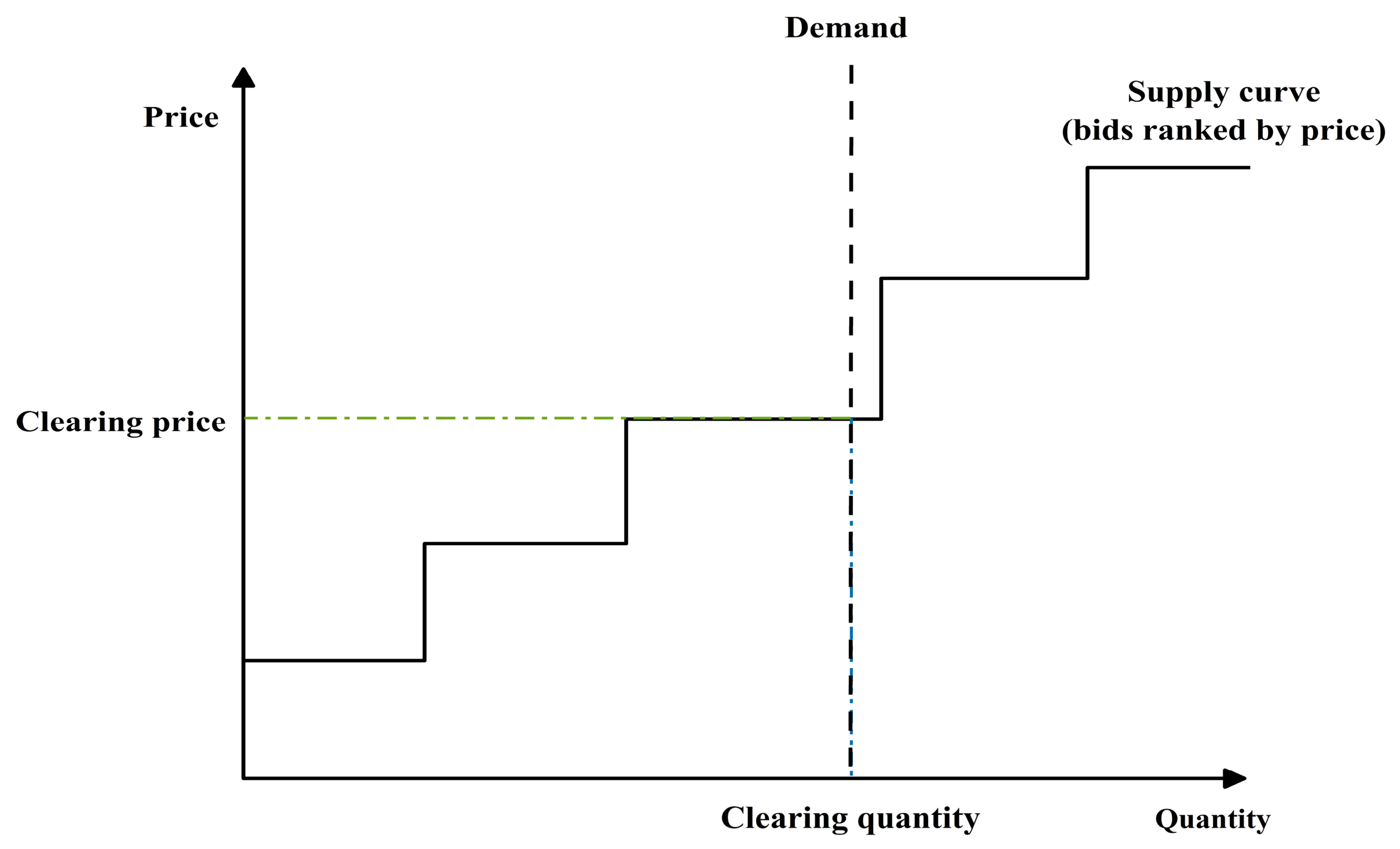
To further promote the marketization of the power industry, China launched a new round of power sector reform in 2015 [27]. The construction of electricity spot markets has become a central component of China’s power-market reform. These spot markets are mainly organized at the provincial level and are designed to improve short-term price discovery, resource allocation and system balancing. In terms of market design, most pilot regions in China have adopted a pool-based market structure [28]. The clearing process generally follows the merit-order principle, as shown in Figure 1. Generation companies (GenCos) submit bid prices and quantities to the Independent System Operator (ISO). The ISO ranks bids from the lowest to the highest price and accumulates offered quantities until electricity demand is satisfied [29,30]. Most pilot spot markets include both day-ahead and real-time markets. The day-ahead market provides a forward schedule based on expected load, generation availability and renewable output. The real-time market then adjusts this schedule in response to load fluctuations, generator outages and other deviations [31]. The sequential operation of day-ahead and real-time markets can improve balancing efficiency, but it also requires prices to respond quickly to changing system conditions. Therefore, whether spot prices can incorporate available information in a timely and complete manner is a key issue in evaluating both market efficiency and the effectiveness of market design.

Against this background, this study investigates the efficiency of China’s electricity spot markets through three representative provincial cases. It aims to assess whether provincial spot prices provide efficient and informative price signals, and to identify the system and market conditions associated with cross-provincial differences in market efficiency. This study makes three main contributions. First, it provides direct empirical evidence on the efficiency of China’s provincial electricity spot markets and thus extends the literature on electricity market efficiency in the context of emerging power market reforms. Second, rather than treating market efficiency as a single property, it evaluates price formation from multiple empirical perspectives, including weak-form efficiency, day-ahead and real-time price convergence, fractal characteristics and sample entropy. Third, it relates the observed cross-provincial differences to intraday load patterns, generation mix, market structure and market design, thereby showing how the quality of price signals in electricity markets is associated with underlying system and market conditions. These findings provide policy-relevant insights for improving market design and supporting the sustainable development of power systems.

2. Methods and Data

This section introduces the theoretical hypotheses and empirical methods used to evaluate market efficiency.

2.1. Theoretical Hypotheses

2.1.1. Efficient Market Hypothesis

Fama proposed the Efficient Market Hypothesis (EMH) to explain market efficiency in financial markets [32]. The EMH states that in a fully competitive and transparent stock market, security prices instantaneously reflect all available information. Under such conditions, investors cannot consistently earn excess returns by analyzing historical price movements, except in the presence of market manipulation or privileged information. According to the EMH, market efficiency can be classified into three forms:

• Weak-form efficiency: Current prices fully reflect all historical information, so future prices cannot be predicted on the basis of past price data alone;
• Semi-strong-form efficiency: Prices adjust rapidly to all publicly available information. Investors therefore cannot obtain excess returns using either historical price data or public information, although those with access to non-public information may still earn abnormal returns;
• Strong-form efficiency: Prices fully reflect all information, both public and private. Under this condition, no investor can systematically earn returns above the normal market level.

Similar to financial markets, electricity market efficiency can also be evaluated from the predictability of price changes. In an efficient electricity market, current electricity prices should fully incorporate all relevant information, making it difficult for market participants to earn excess profits through the use of available information. Therefore, the statistical properties of electricity price series, such as stationarity, volatility and complexity, can provide useful evidence for assessing market efficiency.

It should be noted that traditional measures of market efficiency are generally developed for storable financial assets or commodities. Electricity spot markets are different because electricity is largely non-storable and must be physically balanced in real time [11]. Therefore, predictable electricity prices do not necessarily imply exploitable inter-temporal arbitrage opportunities in the same sense as in financial markets. In this study, market inefficiency primarily refers to statistical predictability and incomplete information incorporation in spot prices. If prices display persistent predictability, low complexity or systematic day-ahead and real-time price gaps, this suggests that prices may not fully and promptly reflect available market and system information. The day-ahead and real-time markets trade the same underlying commodity for delivery at the same time but at different trading horizons, so persistent price differences may indicate imperfect price convergence across market segments [33]. Such evidence should be interpreted as a signal of price-formation quality and market-design effectiveness, rather than as direct evidence of risk-free arbitrage opportunities.

2.1.2. Fractal Market Hypothesis

The efficient market hypothesis assumes that markets are linear and isolated systems, in which returns follow a normal distribution and investors respond linearly to new information. However, in real markets, investors’ reactions to information are often nonlinear and return series commonly exhibit skewness and leptokurtosis [34,35].

The Fractal Market Hypothesis (FMH), proposed by Peters [36], emphasized the heterogeneity of market participants in both information interpretation and investment horizons. As a result, different investors may respond to the same information in different and nonlinear ways [35].

Electricity price series typically exhibit several distinctive features, including seasonality, mean reversion and large price fluctuations. Seasonality is a common statistical characteristic in the electricity market, as prices often vary across seasons and time periods [37,38]. Mean reversion implies that an increase in electricity prices is often followed by a downward adjustment, while a decrease may be followed by an upward correction [18]. At the same time, when price increases or decreases persist over a certain period, electricity prices may also display persistence or long memory. In addition, electricity prices can fluctuate sharply over short periods because of supply and demand shocks [39,40]. Therefore, electricity price dynamics can be regarded as a complex, nonlinear and non-stationary process with typical fractal characteristics [41]. Given these properties, fractal theory has been increasingly applied to quantitatively analyze electricity price series in order to better capture their dynamic behavior and underlying structural features [18,42,43].

2.2. Methods

2.2.1. Efficient Market Hypothesis Test

For electricity spot markets, weak-form efficiency implies that past price movements should not provide systematic forecasting power for future prices [2]. The unit root test is therefore used as a baseline test of whether electricity prices are consistent with a random-walk process. Failure to reject the null hypothesis of unit root suggests that price movements are closer to a random walk, which is consistent with weak-form efficiency. Rejection of the null hypothesis indicates stationarity and mean reversion, implying that historical prices may contain predictive information and the market deviates from weak-form efficiency. Accordingly, this study applies the Augmented Dickey–Fuller (ADF) test [44] to examine the stationarity of electricity price time series, as shown in Equation (1):

$$\Delta {\mathrm{P}}_{\mathrm{t}}=\alpha +{\beta }_0{\mathrm{P}}_{\mathrm{t}-1}+{\beta }_1\Delta {\mathrm{P}}_{\mathrm{t}-1}+{\beta }_2\Delta {\mathrm{P}}_{\mathrm{t}-2}+\cdots +{\beta }_p\Delta {\mathrm{P}}_{\mathrm{t}-\mathrm{p}}+{\mathrm{e}}_{\mathrm{t}},$$

(1)

where $\Delta P_t$ denotes the change in electricity price at time $t$. $\alpha$, ${\beta }_0$, ${\beta }_1\dots {\beta }_p$ are the parameters to be estimated, $P_{t-1}$ is the electricity price at time $t-1$ and $e_t$ is the error term. The lag order in the ADF test is determined according to the Akaike Information Criterion (AIC). The null hypothesis of the ADF test is that the series contains a unit root and is therefore non-stationary. Failure to reject the null hypothesis suggests that the price series follows a random walk process, which is generally regarded as being consistent with weak-form market efficiency.

2.2.2. Price Convergence Test

Following the approaches adopted in [12,17], this paper further evaluates market efficiency based on price convergence between the day-ahead and real-time markets. A persistent price difference between the day-ahead and real-time markets may indicate the existence of arbitrage opportunities across the two markets. In an efficient market with risk-neutral traders and no transaction costs, the day-ahead and real-time electricity prices for delivery at the same time and location should be equal. This implies that the day-ahead price formed at time $t-j$ should incorporate all information available at time $t-j$ regarding the expected real-time price at time $t$, that is,

$$P_t^{t-j}=e^{P_t^t{\Phi }_{t-j}},$$

(2)

where $P_t^{t-j}$ denotes the day-ahead electricity price formed at time $t-j$. $P_t^t$ is the real-time electricity price at time $t$. ${\mathsf{\Phi }}_{t-j}$ represents the information set available at time $t-j$. Therefore, Equation (2) can be rewritten as:

$$P_t^t-P_t^{t-j}=\theta +{\epsilon }_{\mathrm{t}},$$

(3)

where ${\epsilon }_t$ is a white noise error term. If the day-ahead price is an unbiased predictor of the real-time price and fully reflects the information available at time $t-j$, then $\theta$ should be equal to zero. Thus, this study uses Equation (3) to test whether the day-ahead price converges to the real-time price, thereby assessing the efficiency of the electricity spot market. To account for possible heteroscedasticity and autocorrelation in the residuals, Newey–West standard errors are used in the regression estimation.

2.2.3. Fractal Market Hypothesis Test

Following the method used in [45], this study employs Detrended Fluctuation Analysis (DFA) to estimate the Hurst exponent. Compared with the rescaled range (R/S) analysis, DFA generally performs better in the presence of non-stationarity and is more robust for finite samples. By comparing the estimated Hurst exponent $H$ with the benchmark value of 0.5, it is possible to assess whether the electricity price series is consistent with the FMH. If $H=0.5$, the price series follows a random walk, which is generally regarded as being consistent with market efficiency. The specific steps of the DFA procedure are as follows.

Suppose that $x\left(i\right)$ $(i=1,\dots ,N)$ is a time series of length $N$. The cumulative profile of the series is constructed as:

$$y\left(i\right)=\sum _{k=1}^i\left|x\left(k\right)-\overline{x}\right|,$$

(4)

where $\overline{x}={\displaystyle \frac{1}{N}}{\sum }_{i=1}^{N}x\left(i\right)$ is the mean of the original time series. The profile $y\left(i\right)$ is then divided into $N_s=[N/s]$ non-overlapping sub-intervals of equal length $s$. To make full use of the data, the same division procedure is repeated starting from the opposite end of the series, resulting in a total of $2N_s$ sub-intervals. For each sub-interval $v_j (j=\mathrm{1,2},\dots ,N_s)$, a least-squares polynomial fit is used to estimate the local trend,

$$P_j^m\left(k\right)=b_{j0}+b_{j1}k+\cdots +b_{j\left(m-1\right)}{k}^{m-1}+b_{jm}{k}^m\left(m=\mathrm{1,2},\cdots \right).$$

(5)

Next, the detrended series in each sub-interval is calculated as $y_j\left(k\right)=y\left(k\right)-P_j^m\left(k\right)$, where $P_j^m\left(k\right)$ denotes the fitted polynomial trend of order $m$. The variance of each detrended sub-interval, denoted by $F^2\left(s,j\right)$, is defined as

$$F^2\left(s,j\right)={\displaystyle \frac{1}{s}}\sum _{i=1}^s{\left\{y\right[(j-1)s+i]-P_j^m\left(i\right)\}}^2 j=\mathrm{1,2},\dots ,N_s,$$

(6)

$$F^2\left(s,j\right)={\displaystyle \frac{1}{s}}\sum _{i=1}^s{\left\{y\right[N-(j-N_s)s+i]-P_j^m\left(i\right)\}}^2 j=N_s+1,N_s+2,\dots ,2N_s.$$

(7)

Finally, the fluctuation function $F\left(s\right)$ is calculated on the basis of $F^2\left(s,j\right)$,

$$F\left(s\right)={\left[{\displaystyle \frac{1}{2N_s}}\sum _{j=1}^{2N_s}{F}^2\left(s,j\right)\right]}^{1/2}.$$

(8)

The relationship between $F\left(s\right)$ and the scale $s$ follows a power law form, i.e., $F\left(s\right)\propto s^H$. When $H=0.5$, the price series follows a random walk and the market is consistent with efficiency. When $0<H<0.5$, the price series exhibits mean reversion characteristics, meaning that an upward (downward) movement is more likely to be followed by a downward (upward) movement. When $0.5<H<1$, the price series exhibits persistence, meaning that an upward (downward) movement is more likely to be followed by a further upward (downward) movement.

In the empirical implementation, the return series is first demeaned and cumulatively summed to construct the profile. The profile is then divided into non-overlapping windows with different scales $s$ and a first-order polynomial is fitted within each window for detrending, corresponding to DFA−1. Following common practice in the DFA literature [46], the minimum scale is set to 5, the maximum scale is set to one tenth of the sample length and the scale step is 2. To account for statistical uncertainty, we also report 95% confidence intervals for the Hurst exponents. These intervals are calculated from the standard errors of the slope coefficients in the log–log scaling regression between $logF\left(s\right)$ and $log\left(s\right)$.

2.2.4. Trends of Electricity Market Efficiency

This study further employs an entropy-based approach to measure information efficiency and its dynamic evolution in the electricity market. In information theory, entropy quantifies the uncertainty or complexity of a time series by measuring the richness of its underlying patterns. A higher entropy value indicates more efficient information transmission, lower predictability and thus higher market efficiency [47].

For a time series $u=u\left(1\right),u\left(2\right),\dots ,u\left(N\right)$ consisting of $N$ observations, the series is first reconstructed into vectors of dimension $m$ according to the time order. Specifically, $x_m\left(i\right)=\{u\left(i\right),u\left(i+1\right),\dots ,u\left(i+m-1\right)\}$ and $x_m\left(j\right)=\{u\left(j\right),u\left(j+1\right),\dots ,u\left(j+m-1\right)$. The Chebyshev distance between $x_m\left(i\right)$ and $x_m\left(j\right)$ is then calculated as:

$$d\left[x_m\left(i\right),x_m\left(j\right)\right]=\underset{k=\mathrm{1,2},\dots ,m}{\max }\left(\left|u\left(i+k-1\right)-u\left(j+k-1\right)\right|\right).$$

(9)

For a given $x_m\left(i\right)$, let $B_i$ denote the number of vectors $x_m\left(j\right) (1\le j\le N-m, j\ne i)$ whose distance from $x_m\left(i\right)$ is less than or equal to $r$. $B_i$ is defined as

$$B_i^m\left(r\right)={\displaystyle \frac{1}{N-m-1}}{B}_i.$$

(10)

The number of matched vectors $B^m\left(r\right)$ can be calculated by the following equation,

$$B^m\left(r\right)={\displaystyle \frac{1}{N-m}}\sum _{i=1}^{N-m}{B}_i^m\left(r\right).$$

(11)

Similarly, let $A_i$ denote the number of vectors $x_{m+1}\left(j\right) (1\le j\le N-m, j\ne i)$ whose distance from $x_{m+1}\left(i\right)$ is less than or equal to $r$. Then $A_i^m\left(r\right)$ and $A^m\left(r\right)$ are defined as

$$A_i^m\left(r\right)={\displaystyle \frac{1}{N-m-1}}{A}_i,$$

(12)

$$A^m\left(r\right)={\displaystyle \frac{1}{N-m}}\sum _{i=1}^{N-m}{A}_i^m\left(r\right).$$

(13)

Since the number of $A^m\left(r\right)$ is always less than or equal to $B^m\left(r\right)$, the ratio ${\displaystyle \frac{A^m\left(r\right)}{B^m\left(r\right)}}<1$ can be regarded as a conditional probability that two matched sequences of length $m$ remain matched when the dimension increases to $m+1$ [48]. Accordingly, sample entropy is defined as

$$SampEn\left(m,r\right)=\underset{N\to \mathrm{\infty }}{\lim }\left\{-\ln \left[{\displaystyle \frac{A^m\left(r\right)}{B^m\left(r\right)}}\right]\right\}.$$

(14)

For a finite sample $N$, sample entropy can be estimated as,

$$SampEn\left(m,r,N\right)=-\ln \left[{\displaystyle \frac{A^m\left(r\right)}{B^m\left(r\right)}}\right].$$

(15)

2.2.5. Software and Computational Tools

The empirical analysis was implemented using R 4.5.2 and Python 3.13.9. The ADF tests were conducted in R using the urca package, and the day-ahead and real-time price convergence tests were estimated in R using lmtest and sandwich to obtain Newey–West robust standard errors. DFA and sample entropy were implemented in Python, using numpy for numerical calculations, pandas for data processing, matplotlib for visualization and the sampen package for sample entropy calculation.

2.3. Conceptual Framework for Market Efficiency Assessment

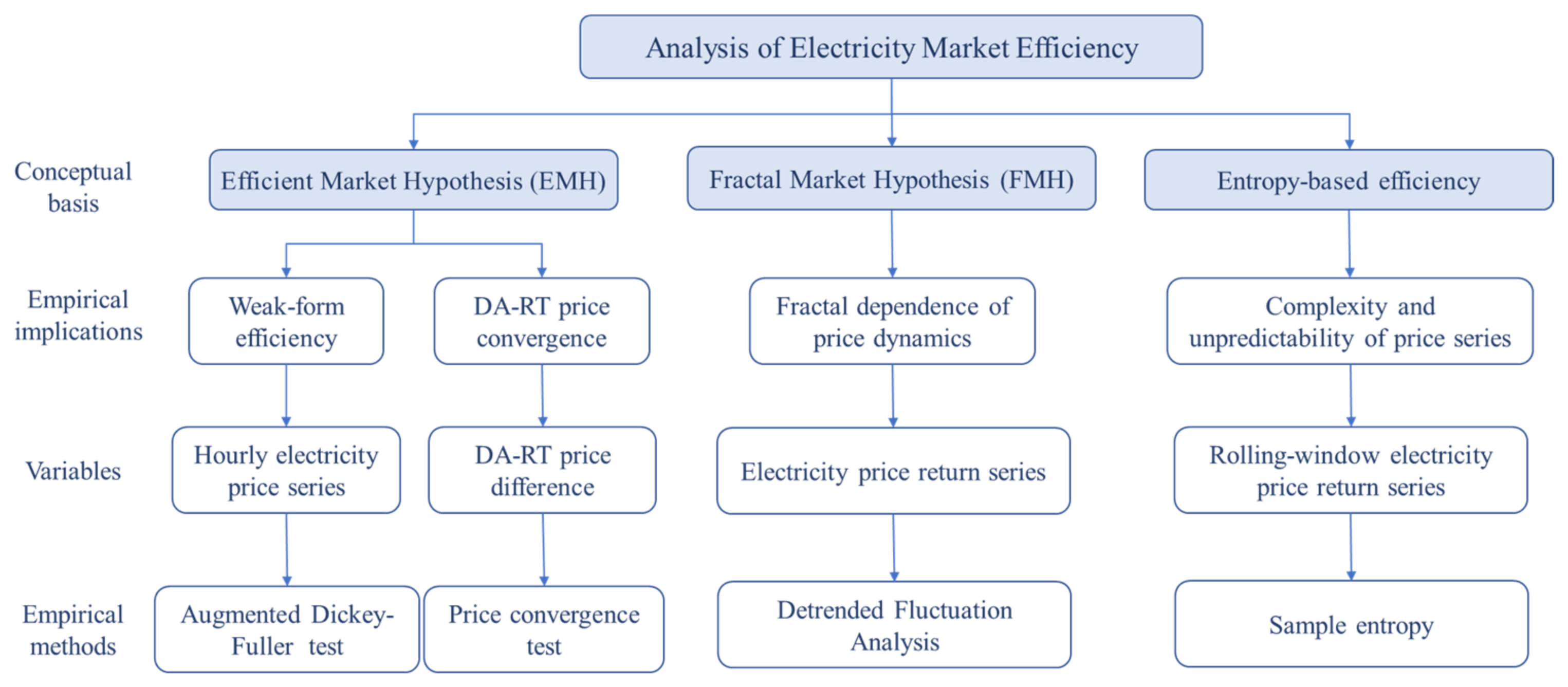
Based on the above theoretical hypotheses and empirical methods, Figure 2 presents the conceptual framework for electricity market efficiency assessment. The Efficient Market Hypothesis is examined from two perspectives: weak-form efficiency and day-ahead–real-time price convergence. The Fractal Market Hypothesis is assessed through the fractal dependence of electricity price returns. In addition, sample entropy is used to evaluate the level and time-varying trend of market efficiency by measuring the complexity and unpredictability of electricity price returns. Together, these complementary perspectives and methods help provide a more structured assessment of electricity market efficiency.

2.4. Electricity Market and Data Description

2.4.1. Background of the Selected Provincial Markets

China’s electricity spot market reform has been implemented mainly through provincial pilot markets. Against this background, this study focuses on Shandong, Shanxi and Guangdong. These three provinces were among the earliest provincial electricity spot markets in China and have accumulated relatively long operating experience. They also differ substantially in thermal-generation structure and emission characteristics. This makes them suitable cases for examining the heterogeneity of electricity market efficiency across China’s provincial spot markets.

In terms of generation structure, Shandong and Shanxi rely heavily on thermal power, especially coal-fired generation, as shown in

Table 1. Basic Information of Thermal Power Plants in Shandong, Shanxi and Guangdong.

	Number of Power Plants	Cumulative Capacity (MW)	Power Generation (Billion kWh)	Coal Consumption (g/kWh)
Shandong
Coal	383	106,010	489.63	268.86
Gas	-	-	-	-
Total	383	106,010	489.63	268.86
Shanxi
Coal	104	67,971	295.08	311.62
Gas	5	1817	4.23	279.76
Total	109	69,788	299.31	310.16
Guangdong
Coal	52	62,395	298.88	300.83
Gas	31	23,651	70.05	240.26
Total	83	86,047	368.93	278.20

Note: Cumulative capacity and power generation are summed across all power plants of different types in each province. Coal consumption values are averages of different types of power plants in each province. Coal consumption is measured in standard coal equivalent. It is used as a comparable energy-efficiency indicator for different thermal generation technologies. All the data are collected from the Compilation of Statistics on the Electric Power Industry.

. Shanxi is a major coal and power-exporting province, while Shandong combines a large thermal-power base with rapid growth in renewable generation, especially photovoltaic power. The low marginal cost and priority dispatch of photovoltaic generation may affect market clearing during periods of high solar output [49]. Guangdong has a more diversified supply structure, with a higher share of gas-fired generation and substantial electricity imports from other provinces. Gas-fired units are generally more flexible but more expensive, which may influence price formation and short-term balancing.

In addition to generation-side differences, the three provinces also represent different regional demand levels. Shandong and Guangdong are large electricity-consuming provinces, while Shanxi has a stronger energy-base characteristic. These differences highlight the diversity of market environments covered by the sample.

2.4.2. Data Sources and Sample Description

The electricity price data are obtained from publicly available sources released by the power trading centers of Shandong, Shanxi and Guangdong. The sample begins with the launch of long-term settlement trial operation in each provincial spot market. Specifically, the Shanxi spot market entered trial operation in April 2021, while the Shandong and Guangdong spot markets began trial operation in November 2021 and December 2021, respectively.

Since the pilot spot markets were launched at different times across provinces, this study uses a common sample period from 1 January 2022 to 31 August 2024 to ensure interprovincial comparability. For each province, the dataset includes both day-ahead and real-time electricity prices at a 15-min frequency. Before the empirical analysis, missing prices were filled using linear interpolation to maintain a regular time series. Negative prices, zero prices, and capped prices were retained because they reflect actual market conditions in electricity spot markets.

Table 2. Descriptive statistics of electricity prices.

Variable	Observations	Mean	Standard Deviation	Skewness	Kurtosis
Shandong DA	93,504	346.724	198.831	−0.356	3.748
Shandong RT	93,504	345.903	230.437	0.191	4.251
Shanxi DA	93,504	365.973	250.438	2.404	11.824
Shanxi RT	93,504	389.713	318.849	2.124	8.144
Guangdong DA	93,504	450.547	152.223	1.013	7.192
Guangdong RT	93,504	459.367	200.353	1.151	6.062

Note: DA denotes the day-ahead market; RT denotes the real-time market.

reports the descriptive statistics of the 15-min electricity prices in Shandong, Shanxi and Guangdong. Each price series contains 93,504 observations. The average day-ahead and real-time electricity prices in Shandong are approximately 346 CNY/MWh (CNY: Chinese Yuan; MWh: Megawatt-hour. CNY/MWh denotes Chinese yuan per megawatt-hour). In Shanxi, the corresponding average prices are 366 CNY/MWh and 390 CNY/MWh, respectively. Guangdong records the highest average price levels among the three provinces, with day-ahead and real-time prices of 451 CNY/MWh and 460 CNY/MWh. It is worth noting that Shandong, Shanxi and Guangdong impose explicit upper and lower limits on spot market quotations. In Shandong, the quotation range is from −100 CNY/MWh to 1500 CNY/MWh, while in Shanxi and Guangdong it ranges from 0 CNY/MWh to 1500 CNY/MWh. The high skewness and kurtosis values, especially in Shanxi, indicate that electricity prices are non-normal, asymmetric and fat-tailed. These distributional features are consistent with the nonlinear and volatile nature of electricity prices, and help motivate the subsequent analysis of price efficiency from stationarity, price convergence, fractal and complexity perspectives.

To account for differences in trading arrangements and short-term price fluctuations across provincial markets, the 15-min price data are aggregated into hourly series in this study. Specifically, the representative electricity price for each hour is calculated as the arithmetic mean of the four 15-min prices within that hour.

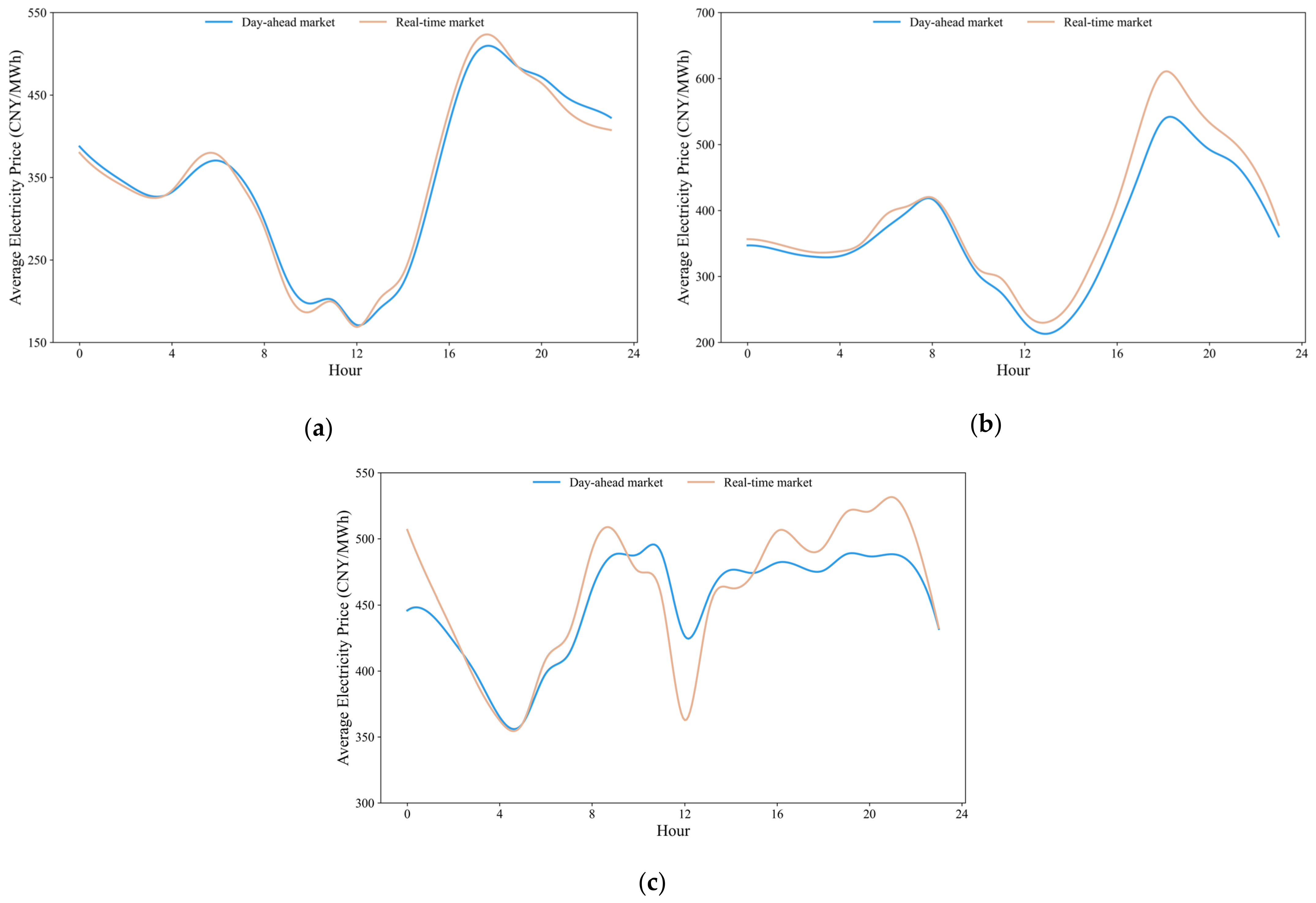
Figure 3 shows the average intraday profiles of day-ahead and real-time electricity prices in Shandong, Shanxi and Guangdong. Prices in all three provinces display clear daily patterns, but their shapes differ across provinces. In Shandong, the day-ahead and real-time curves show broadly similar movements, with prices declining before midday and increasing sharply in the late afternoon. In Shanxi, both curves exhibit a pronounced midday trough and an evening peak, and real-time prices are slightly higher than day-ahead prices in many hours. Guangdong shows a different pattern. The day-ahead price curve displays more moderate intraday variation, while the real-time curve fluctuates more strongly, especially around midday and in the evening.

These patterns suggest heterogeneous day-ahead and real-time market alignment across provinces. Shandong and Shanxi show relatively similar intraday movements between the two markets, although real-time prices tend to exceed day-ahead prices during some peak periods. In Guangdong, the larger real-time fluctuations indicate stronger short-term adjustment needs or greater forecast and balancing uncertainty.

In addition to electricity price data, this study also uses intraday load data, power generation by source and installed-capacity information to interpret cross-provincial heterogeneity in market efficiency. These data are used to construct the load profiles, generation mix and ownership concentration indicators.

Table 3. Variable description and data sources.

Variable	Unit	Data Source	Web Link
Day-ahead price	CNY/MWh	Provincial power trading centers	https://dianchacha.cn/home/ (accessed on 3 April 2026)
Real-time price	CNY/MWh
Load	MW
Power generation	108 kWh	Compilation of Statistics on the Electric Power Industry	-
Installed capacity	MW

Note: Electricity price data are released by provincial power trading centers and accessed through Dianchacha. The Compilation of Statistics on the Electric Power Industry is a printed statistical yearbook. Power generation by source is used to calculate the generation mix, measured as the share of each generation type in total electricity generation. Unit-level installed capacity and ownership information are used to calculate ownership concentration, measured as the installed-capacity share of the five major power generation groups.

summarizes the variables used in this study, including their measurement units, data sources and web links.

3. Results

3.1. Unit Root Test Results

This study first employs unit root tests to assess the market efficiency of electricity spot markets.

Table 4. Unit root test results.

Time	Shandong		Shanxi		Guangdong
	DA	RT	DA	RT	DA	RT
00:00–01:00	−3.533 **	−3.875 **	−6.057 ***	−6.441 ***	−3.540 **	−3.751 **
01:00–02:00	−3.778 **	−3.888 **	−6.334 ***	−6.605 ***	−3.219 *	−3.661 **
02:00–03:00	−3.922 **	−3.856 **	−4.935 ***	−6.682 ***	−3.989 ***	−4.218 ***
03:00–04:00	−5.495 ***	−3.884 **	−4.961 ***	−6.620 ***	−5.638 ***	−4.371 ***
04:00–05:00	−4.010 ***	−3.971 ***	−4.931 ***	−6.954 ***	−5.614 ***	−3.354 *
05:00–06:00	−5.687 ***	−5.565 ***	−4.729 ***	−6.094 ***	−5.301 ***	−3.928 **
06:00–07:00	−6.739 ***	−6.889 ***	−4.457 ***	−4.401 ***	−3.360 *	−3.361 *
07:00–08:00	−10.863 ***	−5.220 ***	−4.865 ***	−4.571 ***	−4.919 ***	−3.521 **
08:00–09:00	−3.814 **	−3.796 **	−3.901 **	−5.269 ***	−3.450 **	−3.036
09:00–10:00	−4.224 ***	−7.864 ***	−4.060 ***	−6.663 ***	−3.871 **	−3.556 **
10:00–11:00	−6.424 ***	−8.707 ***	−3.774 **	−9.486 ***	−3.908 **	−3.249 *
11:00–12:00	−6.567 ***	−9.147 ***	−6.178 ***	−8.387 ***	−3.555 **	−3.184 *
12:00–13:00	−6.375 ***	−8.674 ***	−3.477 ***	−9.024 ***	−3.148 *	−3.206 *
13:00–14:00	−7.226 ***	−8.957 ***	−3.432 **	−8.138 ***	−3.290 *	−3.679 **
14:00–15:00	−6.978 ***	−7.214 ***	−5.103 ***	−8.436 ***	−3.444 **	−6.030 ***
15:00–16:00	−7.009 ***	−4.773 ***	−3.787 **	−7.550 ***	−3.601 **	−4.991 ***
16:00–17:00	−4.348 ***	−4.255 ***	−4.281 ***	−6.559 ***	−4.901 ***	−3.050
17:00–18:00	−4.251 ***	−5.249 ***	−5.798 ***	−6.016 ***	−4.829 ***	−5.016 ***
18:00–19:00	−4.542 ***	−6.822 ***	−6.552 ***	−5.939 ***	−3.185 *	−3.715 **
19:00–20:00	−4.186 ***	−6.006 ***	−6.786 ***	−5.977 ***	−3.336 *	−3.083
20:00–21:00	−4.344 ***	−6.262 ***	−6.480 ***	−5.920 ***	−3.589 **	−4.941 ***
21:00–22:00	−4.387 ***	−4.161 ***	−6.897 ***	−6.695 ***	−5.068 ***	−3.777 **
22:00–23:00	−4.070 ***	−3.930 **	−7.076 ***	−7.301 ***	−3.597 **	−5.782 ***
23:00–24:00	−3.706 **	−4.389 ***	−5.582 ***	−7.052 ***	−3.548 **	−5.864 ***
Efficient hours	0	0	0	0	0	3

Note: *** p < 0.01, ** p < 0.05, * p < 0.1.

shows the hourly unit root results for the day-ahead and real-time electricity markets in Shandong, Shanxi and Guangdong. The null hypothesis of a unit root is rejected in almost all cases, indicating that electricity price series are stationary in most hourly periods across the three provinces. The only exceptions are three hourly periods in the Guangdong real-time market: 8:00–9:00 AM, 4:00–5:00 PM and 7:00–8:00 PM, for which the null hypothesis cannot be rejected. Since stationarity implies that price movements may be at least partly predictable, these results are inconsistent with weak-form market efficiency. Overall, the unit root test results suggest that the electricity spot markets in Shandong, Shanxi and Guangdong generally do not satisfy weak-form efficiency. The robustness results are reported in

Table A1. Unit root test results (2022–2023).

Time	Shandong		Shanxi		Guangdong
	DA	RT	DA	RT	DA	RT
00:00–01:00	−5.161 ***	−4.668 ***	−5.208 ***	−5.211 ***	−2.930	−3.140 *
01:00–02:00	−3.541 **	−3.589 **	−4.217 ***	−5.650 ***	−3.241 *	−3.047
02:00–03:00	−4.812 ***	−3.463 **	−4.079 ***	−5.584 ***	−4.743 ***	−3.494 **
03:00–04:00	−4.664 ***	−3.497 **	−4.144 ***	−5.847 ***	−4.692 ***	−6.193 ***
04:00–05:00	−2.767	−5.067 ***	−4.116 ***	−5.878 ***	−4.732 ***	−5.345 ***
05:00–06:00	−2.767	−4.812 ***	−3.943 **	−5.172 ***	−4.721 ***	−4.965 ***
06:00–07:00	−5.920 ***	−5.871 ***	−3.696 **	−5.097 ***	−2.723	−5.035 ***
07:00–08:00	−9.596 ***	−13.250 ***	−4.122 ***	−3.811 **	−3.942 **	−4.237 ***
08:00–09:00	−6.196 ***	−3.053	−3.195 *	−4.300 ***	−3.256 *	−2.465
09:00–10:00	−7.042 ***	−7.375 ***	−5.267 ***	−5.473 ***	−3.050	−3.040
10:00–11:00	−9.997 ***	−14.425 ***	−5.298 ***	−7.910 ***	−3.032	−2.671
11:00–12:00	−10.100 ***	−14.621 ***	−5.462 ***	−6.979 ***	−2.763	−2.574
12:00–13:00	−6.420 ***	−14.205 ***	−6.501 ***	−7.266 ***	−2.567	−4.080 ***
13:00–14:00	−6.482 ***	−14.693 ***	−4.570 ***	−6.630 ***	−2.729	−3.401 **
14:00–15:00	−6.934 ***	−10.148 ***	−6.567 ***	−6.959 ***	−2.719	−4.764 ***
15:00–16:00	−7.274 ***	−12.093 ***	−4.904 ***	−6.253 ***	−4.467 ***	−4.804 ***
16:00–17:00	−4.280 ***	−4.270 ***	−3.512 **	−6.258 ***	−3.930 **	−4.449 ***
17:00–18:00	−3.997 ***	−4.731 ***	−4.616 ***	−5.068 ***	−3.958 **	−4.133 ***
18:00–19:00	−4.139 ***	−6.154 ***	−5.276 ***	−4.921 ***	−3.858 **	−3.634 **
19:00–20:00	−4.032 ***	−5.512 ***	−5.566 ***	−5.850 ***	−2.720	−2.598
20:00–21:00	−4.078 ***	−5.789 ***	−5.293 ***	−5.790 ***	−2.899	−4.628 ***
21:00–22:00	−4.004 ***	−7.593 ***	−5.639 ***	−5.883 ***	−4.182 ***	−3.050
22:00–23:00	−3.684 **	−3.413 **	−5.575 ***	−6.003 ***	−4.036 ***	−4.854 ***
23:00–24:00	−3.484 **	−4.052 ***	−4.833 ***	−5.379 ***	−2.888	−4.975 ***
Efficient hours	2	1	0	0	11	3

Note: *** p < 0.01, ** p < 0.05, * p < 0.1.

,

Table A2. Phillips–Perron test results.

Time	Shandong		Shanxi		Guangdong
	DA	RT	DA	RT	DA	RT
00:00–01:00	−16.821 ***	−17.303 ***	−16.258 ***	−19.146 ***	−6.406 ***	−9.019 ***
01:00–02:00	−23.370 ***	−23.819 ***	−20.020 ***	−23.271 ***	−9.811 ***	−12.651 ***
02:00–03:00	−22.945 ***	−23.747 ***	−19.243 ***	−22.192 ***	−10.320 ***	−12.666 ***
03:00–04:00	−22.856 ***	−23.642 ***	−19.207 ***	−21.813 ***	−13.510 ***	−13.520 ***
04:00–05:00	−22.903 ***	−23.813 ***	−19.429 ***	−21.840 ***	−14.944 ***	−13.613 ***
05:00–06:00	−22.288 ***	−23.547 ***	−18.682 ***	−22.307 ***	−13.686 ***	−13.691 ***
06:00–07:00	−23.416 ***	−24.964 ***	−18.844 ***	−22.948 ***	−11.650 ***	−13.071 ***
07:00–08:00	−24.868 ***	−24.779 ***	−20.366 ***	−23.076 ***	−11.036 ***	−11.963 ***
08:00–09:00	−19.738 ***	−21.206 ***	−19.575 ***	−21.185 ***	−11.615 ***	−15.010 ***
09:00–10:00	−18.329 ***	−20.699 ***	−19.050 ***	−20.809 ***	−12.019 ***	−16.112 ***
10:00–11:00	−18.362 ***	−21.725 ***	−18.532 ***	−21.461 ***	−11.838 ***	−14.940 ***
11:00–12:00	−17.840 ***	−22.063 ***	−19.443 ***	−21.240 ***	−11.084 ***	−13.862 ***
12:00–13:00	−17.404 ***	−21.154 ***	−19.833 ***	−20.921 ***	−10.230 ***	−11.292 ***
13:00–14:00	−17.119 ***	−21.707 ***	−19.758 ***	−20.393 ***	−10.082 ***	−11.945 ***
14:00–15:00	−16.553 ***	−22.015 ***	−19.680 ***	−20.332 ***	−11.597 ***	−15.872 ***
15:00–16:00	−16.001 ***	−22.848 ***	−18.733 ***	−20.950 ***	−11.167 ***	−15.835 ***
16:00–17:00	−17.156 ***	−23.449 ***	−17.963 ***	−19.945 ***	−11.559 ***	−15.265 ***
17:00–18:00	−19.379 ***	−23.777 ***	−18.064 ***	−19.822 ***	−9.651 ***	−12.118 ***
18:00–19:00	−20.980 ***	−24.457 ***	−18.571 ***	−22.068 ***	−8.150 ***	−12.674 ***
19:00–20:00	−21.493 ***	−24.120 ***	−18.690 ***	−22.511 ***	−8.622 ***	−12.601 ***
20:00–21:00	−22.788 ***	−24.693 ***	−18.120 ***	−23.136 ***	−8.098 ***	−11.734 ***
21:00–22:00	−23.493 ***	−25.820 ***	−18.747 ***	−24.176 ***	−8.635 ***	−13.687 ***
22:00–23:00	−23.686 ***	−25.745 ***	−21.461 ***	−26.042 ***	−8.901 ***	−10.884 ***
23:00–24:00	−26.112 ***	−26.261 ***	−20.607 ***	−24.984 ***	−9.128 ***	−11.075 ***
Efficient hours	0	0	0	0	0	0

Note: The PP statistics are reported as Z-tau statistics. The null hypothesis is that the series has a unit root. *** p < 0.01.

and

Table A3. Zivot–Andrews test results.

Time	Shandong		Shanxi		Guangdong
	DA	RT	DA	RT	DA	RT
00:00–01:00	−4.889 **	−5.522 ***	−5.675 ***	−6.929 ***	−5.637 ***	−5.894 ***
01:00–02:00	−5.138 **	−5.383 ***	−5.878 ***	−7.126 ***	−5.822 ***	−5.562 ***
02:00–03:00	−5.160 **	−5.210 **	−6.354 ***	−7.607 ***	−5.947 ***	−5.859 ***
03:00–04:00	−5.316 **	−5.286 **	−6.683 ***	−7.753 ***	−5.987 ***	−6.101 ***
04:00–05:00	−5.374 ***	−5.323 **	−6.638 ***	−7.667 ***	−5.980 ***	−6.231 ***
05:00–06:00	−5.108 **	−4.937 **	−5.941 ***	−7.254 ***	−5.916 ***	−5.832 ***
06:00–07:00	−5.968 ***	−5.990 ***	−5.347 ***	−6.920 ***	−5.553 ***	−5.818 ***
07:00–08:00	−8.011 ***	−7.676 ***	−6.165 ***	−7.291 ***	−5.427 ***	−5.374 ***
08:00–09:00	−6.043 ***	−6.208 ***	−6.030 ***	−6.523 ***	−5.301 **	−5.144 **
09:00–10:00	−5.859 ***	−6.694 ***	−6.548 ***	−7.203 ***	−5.609 ***	−5.366 ***
10:00–11:00	−6.484 ***	−7.608 ***	−6.481 ***	−7.936 ***	−5.301 **	−5.823 ***
11:00–12:00	−7.003 ***	−8.173 ***	−6.336 ***	−7.474 ***	−5.410 ***	−6.192 ***
12:00–13:00	−6.795 ***	−7.557 ***	−6.608 ***	−6.966 ***	−5.801 ***	−6.123 ***
13:00–14:00	−6.804 ***	−7.677 ***	−6.504 ***	−6.697 ***	−5.401 ***	−6.268 ***
14:00–15:00	−6.451 ***	−7.279 ***	−6.411 ***	−6.853 ***	−5.278 **	−5.882 ***
15:00–16:00	−6.206 ***	−7.564 ***	−6.295 ***	−6.725 ***	−5.264 **	−5.735 ***
16:00–17:00	−5.759 ***	−6.709 ***	−5.874 ***	−6.323 ***	−5.347 ***	−5.440 ***
17:00–18:00	−5.633 ***	−6.257 ***	−6.083 ***	−6.394 ***	−5.454 ***	−5.294 **
18:00–19:00	−5.432 ***	−6.468 ***	−5.975 ***	−6.595 ***	−5.319 **	−5.384 ***
19:00–20:00	−5.081 **	−5.969 ***	−6.234 ***	−6.671 ***	−5.229 **	−5.316 **
20:00–21:00	−5.208 **	−6.127 ***	−6.069 ***	−6.623 ***	−5.416 ***	−5.351 ***
21:00–22:00	−5.100 **	−6.479 ***	−5.947 ***	−6.805 ***	−5.489 ***	−5.274 **
22:00–23:00	−4.989 **	−6.140 ***	−6.206 ***	−7.506 ***	−5.377 ***	−5.660 ***
23:00–24:00	−5.051 **	−5.915 ***	−5.594 ***	−7.307 ***	−5.696 ***	−6.257 ***
Efficient hours	0	0	0	0	0	0

Note: For the Zivot–Andrews test, the null hypothesis is a unit root without a structural break. The Zivot–Andrews test allows for an endogenous intercept break and includes 12 lag terms. *** p < 0.01, ** p < 0.05.

.

This study further examines market efficiency on a yearly basis, as shown in

Table 5. Annual unit root test results for the Shandong electricity spot market.

Time	2022		2023		2024
	DA	RT	DA	RT	DA	RT
00:00–01:00	−4.082 ***	−3.074	−4.131 ***	−3.849 **	−7.042 ***	−5.169 ***
01:00–02:00	−5.098 ***	−3.135 *	−5.067 ***	−5.703 ***	−7.694 ***	−4.665 ***
02:00–03:00	−3.238 *	−3.469 **	−4.981 ***	−5.635 ***	−7.562 ***	−4.286 ***
03:00–04:00	−3.001	−3.467 **	−5.003 ***	−2.759	−7.500 ***	−4.845 ***
04:00–05:00	−3.029	−3.389 *	−2.290	−4.205 ***	−5.399 ***	−4.317 ***
05:00–06:00	−3.126	−3.072	−2.260	−4.085 ***	−4.636 ***	−4.196 ***
06:00–07:00	−5.040 ***	−3.775 **	−2.451	−9.510 ***	−4.806 ***	−4.958 ***
07:00–08:00	−7.922 ***	−9.549 ***	−8.920 ***	−9.218 ***	−4.951 ***	−5.320 ***
08:00–09:00	−2.620	−4.227 ***	−8.149 ***	−2.108	−4.724 ***	−3.843 **
09:00–10:00	−5.869 ***	−4.824 ***	−8.354 ***	−8.926 ***	−7.140 ***	−3.851 **
10:00–11:00	−4.634 ***	−6.772 ***	−8.698 ***	−9.634 ***	−7.449 ***	−8.322 ***
11:00–12:00	−4.531 ***	−6.323 ***	−8.934 ***	−9.483 ***	−7.396 ***	−8.647 ***
12:00–13:00	−4.194 ***	−5.839 ***	−8.832 ***	−10.162 ***	−7.365 ***	−8.502 ***
13:00–14:00	−4.208 ***	−6.326 ***	−8.933 ***	−10.452 ***	−7.318 ***	−8.832 ***
14:00–15:00	−4.309 ***	−6.408 ***	−8.607 ***	−10.433 ***	−7.128 ***	−8.986 ***
15:00–16:00	−4.744 ***	−7.963 ***	−8.604 ***	−10.929 ***	−6.572 ***	−8.378 ***
16:00–17:00	−7.971 ***	−8.348 ***	−8.791 ***	−11.669 ***	−6.127 ***	−8.035 ***
17:00–18:00	−2.983	−3.140 *	−5.987 ***	−10.915 ***	−8.010 ***	−8.375 ***
18:00–19:00	−2.437	−3.742 **	−6.021 ***	−10.154 ***	−6.722 ***	−8.350 ***
19:00–20:00	−3.524 **	−3.954 **	−5.523 ***	−4.740 ***	−6.555 ***	−8.002 ***
20:00–21:00	−3.619 **	−11.695 ***	−4.647 ***	−4.787 ***	−6.732 ***	−8.111 ***
21:00–22:00	−2.944	−12.187 ***	−3.721 **	−4.570 ***	−6.805 ***	−4.581 ***
22:00–23:00	−2.557	−7.353 ***	−3.435 **	−4.273 ***	−9.253 ***	−6.434 ***
23:00–24:00	−6.140 ***	−3.400 **	−3.767 **	−4.755 ***	−9.286 ***	−4.418 ***
Efficient hours	8	2	3	2	0	0

Note: *** p < 0.01, ** p < 0.05, * p < 0.1.

,

Table 6. Annual unit root test results for the Shanxi electricity spot market.

Time	2022		2023		2024
	DA	RT	DA	RT	DA	RT
00:00–01:00	−3.760 **	−3.687 **	−6.595 ***	−7.303 ***	−7.370 ***	−7.933 ***
01:00–02:00	−3.099	−3.770 **	−7.600 ***	−5.289 ***	−7.638 ***	−8.154 ***
02:00–03:00	−4.167 ***	−4.002 ***	−9.509 ***	−5.264 ***	−5.443 ***	−7.656 ***
03:00–04:00	−4.182 ***	−4.152 ***	−6.737 ***	−5.717 ***	−5.424 ***	−7.891 ***
04:00–05:00	−3.362 *	−4.697 ***	−6.610 ***	−8.619 ***	−5.625 ***	−3.727 **
05:00–06:00	−3.981 ***	−4.315 ***	−6.585 ***	−9.215 ***	−5.361 ***	−7.819 ***
06:00–07:00	−3.597 **	−3.880 **	−7.858 ***	−8.421 ***	−6.721 ***	−8.203 ***
07:00–08:00	−3.029	−4.498 ***	−5.049 ***	−7.453 ***	−3.080	−8.289 ***
08:00–09:00	−2.250	−3.636 **	−2.997	−3.732 **	−2.985	−8.687 ***
09:00–10:00	−3.844 **	−3.890 **	−3.989 ***	−3.898 **	−7.893 ***	−8.635 ***
10:00–11:00	−3.133 *	−3.718 **	−7.158 ***	−6.923 ***	−6.830 ***	−8.155 ***
11:00–12:00	−3.021	−3.501 **	−7.071 ***	−6.835 ***	−6.770 ***	−8.144 ***
12:00–13:00	−3.468 **	−3.525 **	−5.252 ***	−6.571 ***	−6.906 ***	−7.885 ***
13:00–14:00	−2.655	−3.231 *	−5.907 ***	−6.866 ***	−5.543 ***	−8.178 ***
14:00–15:00	−3.372 *	−3.261 *	−5.356 ***	−7.650 ***	−6.732 ***	−8.373 ***
15:00–16:00	−3.195 *	−4.053 ***	−7.228 ***	−8.020 ***	−5.759 ***	−3.071
16:00–17:00	−2.923	−5.231 ***	−7.603 ***	−4.629 ***	−7.011 ***	−3.793 **
17:00–18:00	−3.163 *	−9.669 ***	−4.776 ***	−3.343 *	−5.328 ***	−2.675
18:00–19:00	−3.552 **	−4.269 ***	−4.863 ***	−6.410 ***	−5.244 ***	−4.483 ***
19:00–20:00	−3.676 **	−3.629 **	−7.409 ***	−10.338 ***	−4.019 ***	−3.420 *
20:00–21:00	−3.468 **	−3.613 **	−4.557 ***	−3.578 **	−2.688	−3.473 **
21:00–22:00	−4.489 ***	−3.930 **	−4.883 ***	−8.321 ***	−2.664	−2.570
22:00–23:00	−3.504 **	−4.822 ***	−7.745 ***	−8.544 ***	−3.898 **	−3.784 **
23:00–24:00	−3.614 **	−4.185 ***	−6.209 ***	−7.823 ***	−6.066 ***	−4.330 ***
Efficient hours	6	0	1	0	4	3

Note: *** p < 0.01, ** p < 0.05, * p < 0.1.

and

Table 7. Annual unit root test results for the Guangdong electricity spot market.

Time	2022		2023		2024
	DA	RT	DA	RT	DA	RT
00:00–01:00	−5.161 ***	−1.679	−2.155	−7.787 ***	−5.190 ***	−6.531 ***
01:00–02:00	−5.172 ***	−3.547 **	−5.414 ***	−2.458	−5.714 ***	−9.549 ***
02:00–03:00	−4.381 ***	−4.097 ***	−3.379 *	−6.386 ***	−6.226 ***	−4.910 ***
03:00–04:00	−2.913	−3.979 ***	−3.184 *	−6.375 ***	−6.374 ***	−5.822 ***
04:00–05:00	−3.867 **	−4.362 ***	−3.242 *	−7.379 ***	−3.844 **	−5.454 ***
05:00–06:00	−3.705 **	−3.722 **	−2.838	−4.238 ***	−2.474	−4.467 ***
06:00–07:00	−3.441 **	−4.063 ***	−2.122	−3.524 **	−6.089 ***	−6.647 ***
07:00–08:00	−3.918 **	−3.084	−1.682	−2.282	−6.088 ***	−4.607 ***
08:00–09:00	−3.648 **	−3.577 ***	−0.959	−2.335	−4.839 ***	−4.298 ***
09:00–10:00	−2.789	−2.139	−2.168	−1.905	−7.274 ***	−6.551 ***
10:00–11:00	−1.993	−3.256 *	−2.343	−3.505 **	−7.296 ***	−3.714 **
11:00–12:00	−1.804	−2.124	−2.489	−3.236 *	−7.472 ***	−6.872 ***
12:00–13:00	−4.684 ***	−2.234	−3.586 **	−7.803 ***	−9.188 ***	−5.926 ***
13:00–14:00	−3.031	−2.827	−3.775 **	−7.797 ***	−8.185 ***	−5.699 ***
14:00–15:00	−2.989	−2.987	−3.614 **	−4.918 ***	−7.357 ***	−5.416 ***
15:00–16:00	−3.048	−2.992	−3.476 **	−4.566 ***	−8.141 ***	−7.516 ***
16:00–17:00	−2.766	−2.803	−2.776	−4.258 ***	−8.351 ***	−3.887 ***
17:00–18:00	−3.000	−3.419 *	−2.342	−3.273 *	−7.883 ***	−8.129 ***
18:00–19:00	−2.957	−3.297 *	−1.973	−2.918	−7.172 ***	−7.509 ***
19:00–20:00	−2.855	−3.158 *	−1.834	−3.347 *	−7.581 ***	−7.096 ***
20:00–21:00	−4.942 ***	−3.254 *	−1.915	−3.784 **	−5.139 ***	−8.635 ***
21:00–22:00	−5.254 ***	−3.069	−2.081	−1.514	−5.688 ***	−8.279 ***
22:00–23:00	−5.199 ***	−3.320 *	−1.345	−5.983 ***	−5.370 ***	−8.377 ***
23:00–24:00	−5.195 ***	−3.760 **	−5.187 ***	−7.305 ***	−4.426 ***	−8.483 ***
Efficient hours	11	10	15	6	1	0

Note: *** p < 0.01, ** p < 0.05, * p < 0.1.

.

Table 5 presents the annual unit root test results for the Shandong electricity spot market. In 2022, the day-ahead and real-time markets satisfy weak-form efficiency in 8 and 2 hourly periods, respectively. In 2023, only 3 hourly periods in the day-ahead market remain weak-form efficient, while the null hypothesis is rejected in almost all other periods. The results in 2024 indicate that neither the day-ahead market nor the real-time market satisfies weak-form efficiency in any hourly period. The limited efficient hours in Shandong mainly occur during low-demand periods, such as 3:00 AM to 6:00 AM. Given that the electricity consumption in Shandong has grown rapidly since 2022, the increase in load may have intensified market tightness and caused electricity prices to deviate further from competitive benchmarks [50].

As shown in Table 6, six hourly periods in the day-ahead market satisfy weak-form efficiency, whereas none of the hourly periods in the real-time market do so in 2022. In 2023, the null hypothesis cannot be rejected in only one hourly period in the day-ahead market, while it is rejected in all other periods. The unit root test results in 2024 show 4 weak-form efficient hours in the day-ahead market and 3 in the real-time market. Since thermal power generation in Shanxi is dominated by coal-fired units, coal prices directly affect generation costs and electricity prices. The relatively low market efficiency observed in 2022 and 2023 may therefore be related to persistently high coal prices during this period. As coal prices gradually returned to more normal levels, market efficiency appears to have improved slightly in 2024.

Table 7 reports the annual unit root test results for the Guangdong electricity spot market. In 2022, the day-ahead market recorded 11 weak-form efficient hours, while the real-time market recorded 10. In 2023, the number of non-stationary hours in the day-ahead market and the real-time market increased to 15 and 6, indicating relatively higher market efficiency than in the other two provinces. However, market efficiency in Guangdong declined in 2024, with only one weak-form efficient hour in the day-ahead market and none in the real-time market. Although Guangdong exhibits more non-stationary hours in certain years, these patterns may not be stable across time and do not overturn the full-sample conclusion of weak-form inefficiency.

Taken together, the annual unit root test results show that none of the three provincial electricity spot markets fully satisfies the weak-form Efficient Market Hypothesis. From the perspective of weak-form efficiency, the widespread stationarity of electricity prices implies that historical price information still contains useful signals for future price movements. Therefore, the observed stationarity can be regarded as evidence that price formation in these provincial spot markets has not yet fully eliminated predictable components. This provides direct empirical support for the conclusion that weak-form efficiency remains limited. Nevertheless, Guangdong exhibits more non-stationary hours than Shandong and Shanxi in several years, suggesting that its price dynamics are relatively closer to the random-walk benchmark.

3.2. Convergence Between Day-Ahead and Real-Time Electricity Prices

Table 8. Convergence test results for day-ahead and real-time electricity prices.

Time	Shandong	Shanxi	Guangdong
00:00–01:00	7.642 **	−9.484 *	−60.829 ***
	(3.675)	(5.180)	(5.613)
01:00–02:00	7.306 **	−9.029 *	−22.488 ***
	(3.692)	(5.015)	(4.513)
02:00–03:00	5.136	−8.318	−6.267
	(3.538)	(5.051)	(4.515)
03:00–04:00	2.336	−6.793	5.906
	(3.165)	(5.024)	(4.213)
04:00–05:00	−2.047	−7.172	2.559
	(3.049)	(5.498)	(4.757)
05:00–06:00	−11.071 ***	−5.951	−0.130
	(3.941)	(5.314)	(4.341)
06:00–07:00	−6.920 **	−19.861 ***	−10.784 ***
	(3.242)	(6.147)	(3.357)
07:00–08:00	7.530 **	−6.932	−15.835 ***
	(3.117)	(6.093)	(4.271)
08:00–09:00	8.742 ***	−2.372	−29.769 ***
	(3.185)	(6.917)	(5.654)
09:00–10:00	14.161 ***	−9.167	−16.843 ***
	(3.905)	(6.725)	(5.637)
10:00–11:00	9.945 **	−8.692	12.985 ***
	(4.721)	(7.471)	(4.875)
11:00–12:00	2.388	−21.939 ***	32.959 ***
	(5.583)	(7.766)	(4.748)
12:00–13:00	2.432	−15.509 **	63.577 ***
	(5.454)	(6.426)	(4.836)
13:00–14:00	−11.830 **	−17.666 ***	11.713 ***
	(5.782)	(5.960)	(4.554)
14:00–15:00	−11.438 **	−24.009 ***	13.835 ***
	(5.231)	(6.531)	(5.015)
15:00–16:00	−18.535 ***	−36.876 ***	−0.603
	(4.965)	(6.803)	(5.431)
16:00–17:00	−17.122 ***	−42.707 ***	−23.851 ***
	(4.712)	(8.489)	(5.495)
17:00–18:00	−14.750 ***	−69.165 ***	−16.763 ***
	(4.929)	(10.043)	(4.774)
18:00–19:00	−11.839 **	−72.374 ***	−17.556 ***
	(5.190)	(9.936)	(5.518)
19:00–20:00	0.084	−52.097 ***	−31.865 ***
	(5.515)	(10.029)	(6.009)
20:00–21:00	7.408	−41.033 ***	−34.122 ***
	(5.900)	(9.445)	(6.090)
21:00–22:00	14.990 ***	−32.113 ***	−43.254 ***
	(5.358)	(9.230)	(6.573)
22:00–23:00	20.130 ***	−31.988 ***	−23.526 ***
	(4.984)	(8.420)	(5.581)
23:00–24:00	15.024 ***	−17.575 ***	−0.742
	(5.017)	(6.272)	(4.797)
Percentage of hours with price convergence	29%	33%	25%

Note: *** p < 0.01, ** p < 0.05, * p < 0.1. Rejecting the null hypothesis indicates a significant difference between day-ahead and real-time prices. The numbers in parentheses represent Newey–West standard errors.

presents the hourly convergence test results for day-ahead and real-time electricity prices. The results show that day-ahead and real-time electricity prices converge for 7, 8 and 5 hourly periods in the Shandong, Shanxi and Guangdong spot markets, corresponding to convergence ratios of 29%, 33% and 25%. Among the three provinces, Shanxi exhibits the highest share of convergent hours, while Guangdong shows the lowest.

The relatively higher convergence ratio in Shanxi may partly reflect its more homogeneous generation mix, which could make real-time operating conditions easier to anticipate in the day-ahead market. By contrast, Guangdong has a more complex power system, with a larger share of gas-fired units and greater load variability. These characteristics may be associated with greater deviations between real-time prices and day-ahead expectations, which could help explain its lower convergence ratio. Robustness tests are shown in

Table A4. Robustness check of the convergence test under alternative Newey–West lags.

Time	Shandong		Shanxi		Guangdong
	Lag = 7	Lag = 14	Lag = 7	Lag = 14	Lag = 7	Lag = 14
00:00–01:00	7.642 **	7.642 *	−9.484 *	−9.484	−60.829 ***	−60.829 ***
	(3.781)	(4.404)	(5.311)	(5.902)	(5.768)	(6.436)
01:00–02:00	7.306 *	7.306 *	−9.029 *	−9.029	−22.488 ***	−22.488 ***
	(3.785)	(4.235)	(5.129)	(5.612)	(4.613)	(5.161)
02:00–03:00	5.136	5.136	−8.318	−8.318	−6.267	−6.267
	(3.621)	(3.932)	(5.154)	(5.620)	(4.601)	(5.024)
03:00–04:00	2.336	2.336	−6.793	−6.793	5.906	5.906
	(3.233)	(3.414)	(5.134)	(5.562)	(4.276)	(4.598)
04:00–05:00	−2.047	−2.047	−7.172	−7.172	2.559	2.559
	(3.133)	(3.362)	(5.624)	(6.163)	(4.866)	(5.294)
05:00–06:00	−11.071 ***	−11.071 **	−5.951	−5.951	−0.130	−0.130
	(4.094)	(4.767)	(5.387)	(5.741)	(4.443)	(4.901)
06:00–07:00	−6.920 **	−6.920 *	−19.861 ***	−19.861 ***	−10.784 ***	−10.784 ***
	(3.333)	(3.725)	(6.290)	(7.023)	(3.393)	(3.639)
07:00–08:00	7.530 **	7.530 **	−6.932	−6.932	−15.835 ***	−15.835 ***
	(3.184)	(3.585)	(6.204)	(6.803)	(4.428)	(5.243)
08:00–09:00	8.742 ***	8.742 ***	−2.372	−2.372	−29.769 ***	−29.769 ***
	(3.200)	(3.301)	(7.067)	(7.920)	(5.872)	(6.927)
09:00–10:00	14.161 ***	14.161 ***	−9.167	−9.167	−16.843 ***	−16.843 ***
	(3.910)	(3.947)	(6.766)	(6.983)	(5.786)	(6.464)
10:00–11:00	9.945 **	9.945 **	−8.692	−8.692	12.985 ***	12.985 **
	(4.769)	(4.964)	(7.568)	(7.906)	(4.937)	(5.220)
11:00–12:00	2.388	2.388	−21.939 ***	−21.939 ***	32.959 ***	32.959 ***
	(5.685)	(6.193)	(7.860)	(8.223)	(4.799)	(4.970)
12:00–13:00	2.432	2.432	−15.509 **	−15.509 **	63.577 ***	63.577 ***
	(5.531)	(6.037)	(6.509)	(6.773)	(4.928)	(5.295)
13:00–14:00	−11.830 **	−11.830 *	−17.666 ***	−17.666 ***	11.713 **	11.713 **
	(5.898)	(6.695)	(5.996)	(6.211)	(4.671)	(5.269)
14:00–15:00	−11.438 **	−11.438 **	−24.009 ***	−24.009 ***	13.835 ***	13.835 ***
	(5.316)	(5.817)	(6.566)	(6.594)	(5.019)	(5.086)
15:00–16:00	−18.535 ***	−18.535 ***	−36.876 ***	−36.876 ***	−0.603	−0.603
	(5.036)	(5.418)	(6.869)	(7.046)	(5.420)	(5.427)
16:00–17:00	−17.122 ***	−17.122 ***	−42.707 ***	−42.707 ***	−23.851 ***	−23.851 ***
	(4.815)	(5.345)	(8.648)	(9.485)	(5.580)	(6.192)
17:00–18:00	−14.750 ***	−14.750 ***	−69.165 ***	−69.165 ***	−16.763 ***	−16.763 ***
	(5.028)	(5.538)	(10.221)	(11.798)	(4.889)	(5.759)
18:00–19:00	−11.839 **	−11.839 **	−72.374 ***	−72.374 ***	−17.556 ***	−17.556 **
	(5.297)	(5.855)	(10.067)	(11.402)	(5.701)	(6.834)
19:00–20:00	0.084	0.084	−52.097 ***	−52.097 ***	−31.865 ***	−31.865 ***
	(5.653)	(6.358)	(10.128)	(11.137)	(6.170)	(7.093)
20:00–21:00	7.408	7.408	−41.033 ***	−41.033 ***	−34.122 ***	−34.122 ***
	(6.044)	(6.850)	(9.568)	(10.303)	(6.229)	(6.979)
21:00–22:00	14.990 ***	14.990 **	−32.113 ***	−32.113 ***	−43.254 ***	−43.254 ***
	(5.474)	(6.106)	(9.386)	(10.068)	(6.721)	(7.648)
22:00–23:00	20.130 ***	20.130 ***	−31.988 ***	−31.988 ***	−23.526 ***	−23.526 ***
	(5.112)	(5.710)	(8.636)	(9.755)	(5.968)	(6.615)
23:00–24:00	15.024 ***	15.024 **	−17.575 ***	−17.575 **	−0.742	−0.742
	(5.162)	(5.927)	(6.430)	(7.245)	(4.874)	(5.350)
Percentage of hours with price convergence	29%	29%	33%	42%	25%	25%

Note: *** p < 0.01, ** p < 0.05, * p < 0.1. Rejecting the null hypothesis indicates a significant difference between day-ahead and real-time prices. The numbers in parentheses represent Newey–West standard errors.

.

Overall, the relatively low shares of convergent hours indicate limited consistency between day-ahead and real-time prices. This finding is relevant for evaluating market efficiency because the convergence test examines whether information is transmitted effectively between the day-ahead and real-time markets. If the day-ahead market fully incorporated expectations about real-time system conditions, systematic deviations between the two prices should be limited. These price differences should also be understood in the operational context of electricity spot markets. Real-time balancing costs, flexibility scarcity, renewable output deviations and unexpected system conditions can all widen the gap between day-ahead and real-time prices. Therefore, the low convergence ratios may indicate limited cross-market price alignment, while also reflecting real-time operational uncertainty and flexibility constraints.

The year-by-year results, reported in

Table A5. Annual day-ahead and real-time electricity price convergence test in Shandong.

Time	2022	2023	2024
00:00–01:00	−1.814	6.614 *	23.324 ***
	(7.318)	(3.536)	(6.326)
01:00–02:00	0.443	8.019 *	16.505 **
	(7.237)	(4.174)	(6.380)
02:00–03:00	−0.808	6.451	12.059 *
	(6.219)	(4.973)	(6.419)
03:00–04:00	−3.550	4.224	8.316
	(4.923)	(4.918)	(6.259)
04:00–05:00	−9.516 *	−1.468	8.259
	(5.323)	(4.274)	(5.381)
05:00–06:00	−18.742 **	−13.975 ***	4.747
	(8.121)	(4.869)	(4.506)
06:00–07:00	−8.819	−13.058 ***	5.101
	(6.553)	(4.309)	(4.098)
07:00–08:00	15.054 **	−6.470	17.218 ***
	(5.979)	(4.008)	(4.479)
08:00–09:00	15.358 **	−3.496	17.151 ***
	(6.227)	(4.139)	(5.240)
09:00–10:00	12.741 *	7.364	26.453 ***
	(7.356)	(5.785)	(6.752)
10:00–11:00	3.203	4.246	28.554 ***
	(8.741)	(6.707)	(8.701)
11:00–12:00	−10.342	−1.734	27.596 ***
	(10.034)	(7.862)	(10.265)
12:00–13:00	−13.805	2.762	26.226 ***
	(9.715)	(7.992)	(9.645)
13:00–14:00	−29.744 ***	−12.072	15.328
	(10.270)	(7.905)	(10.442)
14:00–15:00	−19.548 **	−16.905 **	8.872
	(8.624)	(7.114)	(11.232)
15:00–16:00	−8.667	−37.153 ***	−5.444
	(7.644)	(7.016)	(11.215)
16:00–17:00	−11.482	−27.290 ***	−10.350
	(8.140)	(6.519)	(9.462)
17:00–18:00	−10.049	−22.212 ***	−10.618
	(9.354)	(6.052)	(8.744)
18:00–19:00	−13.366	−14.711 **	−5.260
	(10.688)	(6.410)	(7.723)
19:00–20:00	−5.720	0.548	8.071
	(11.671)	(6.313)	(7.900)
20:00–21:00	−2.925	14.944 **	11.593
	(12.639)	(6.044)	(8.880)
21:00–22:00	3.021	22.320 ***	21.931 **
	(10.779)	(5.639)	(9.628)
22:00–23:00	10.601	22.162 ***	31.342 ***
	(8.798)	(6.170)	(10.092)
23:00–24:00	3.773	14.095 **	33.244 ***
	(9.596)	(5.995)	(8.393)
Efficiency (%)	58%	58%	29%

Note: *** p < 0.01, ** p < 0.05, * p < 0.1. Rejecting the null hypothesis indicates a significant difference between day-ahead and real-time prices. The numbers in parentheses represent Newey–West standard errors.

,

Table A6. Annual day-ahead and real-time electricity price convergence test in Shanxi.

Time	2022	2023	2024
00:00–01:00	−6.271	−13.620 **	−8.103
	(11.359)	(5.783)	(5.956)
01:00–02:00	−2.538	−16.529 ***	−7.520
	(10.671)	(6.247)	(5.472)
02:00–03:00	−2.090	−16.978 ***	−4.678
	(10.856)	(6.050)	(5.858)
03:00–04:00	−0.474	−13.156 **	−6.728
	(10.825)	(5.555)	(6.904)
04:00–05:00	0.834	−10.993 **	−13.432
	(12.002)	(5.402)	(8.231)
05:00–06:00	−4.968	−9.282	−2.437
	(11.792)	(5.794)	(6.876)
06:00–07:00	−32.259 **	−21.256 ***	0.770
	(13.064)	(8.041)	(5.657)
07:00–08:00	−11.964	−12.805	9.378
	(12.688)	(7.906)	(7.986)
08:00–09:00	−4.657	−6.671	7.477
	(14.685)	(8.550)	(8.980)
09:00–10:00	−7.766	−10.339	−9.507
	(13.833)	(9.135)	(9.698)
10:00–11:00	−3.935	−20.183 *	1.382
	(13.832)	(12.096)	(10.200)
11:00–12:00	−24.427 *	−28.310 **	−8.686
	(13.954)	(13.510)	(9.439)
12:00–13:00	−22.909 *	−3.296	−22.709 **
	(11.853)	(9.797)	(10.229)
13:00–14:00	−23.999 **	−5.447	−26.470 ***
	(11.785)	(8.339)	(9.592)
14:00–15:00	−21.672 *	−23.887 **	−27.685 ***
	(11.454)	(11.388)	(9.865)
15:00–16:00	−38.819 ***	−40.523 ***	−28.512 ***
	(12.912)	(11.605)	(7.110)
16:00–17:00	−71.182 ***	−37.480 ***	−7.932
	(17.285)	(12.212)	(6.847)
17:00–18:00	−116.154 ***	−57.982 ***	−15.601 *
	(19.499)	(14.680)	(8.767)
18:00–19:00	−117.507 ***	−56.925 ***	−27.971 **
	(18.540)	(14.101)	(13.473)
19:00–20:00	−98.931 ***	−30.103 **	−14.938
	(18.593)	(13.927)	(14.496)
20:00–21:00	−70.259 ***	−28.708 **	−15.751
	(19.188)	(12.829)	(11.730)
21:00–22:00	−51.320 **	−29.652 ***	−7.062
	(19.903)	(11.060)	(11.638)
22:00–23:00	−40.465 **	−37.656 ***	−10.830
	(18.310)	(10.009)	(9.530)
23:00–24:00	−24.504 *	−17.535 ***	−7.270
	(13.947)	(6.550)	(7.598)
Efficiency (%)	58%	25%	50%

Note: *** p < 0.01, ** p < 0.05, * p < 0.1. Rejecting the null hypothesis indicates a significant difference between day-ahead and real-time prices. The numbers in parentheses represent Newey–West standard errors.

and

Table A7. Annual day-ahead and real-time electricity price convergence test in Guangdong.

Time	2022	2023	2024
00:00–01:00	−48.842 ***	−77.881 ***	−53.251 ***
	(8.630)	(9.427)	(9.036)
01:00–02:00	−24.077 **	−31.031 ***	−7.333
	(9.600)	(5.541)	(4.862)
02:00–03:00	−10.807	−12.189 **	9.382 *
	(9.647)	(5.203)	(5.175)
03:00–04:00	−4.135	1.993	26.777 ***
	(8.493)	(5.283)	(5.236)
04:00–05:00	−21.839 **	4.879	35.586 ***
	(9.107)	(5.432)	(5.639)
05:00–06:00	−22.737 ***	0.240	33.135 ***
	(7.666)	(5.351)	(5.989)
06:00–07:00	−24.640 ***	−12.703 ***	12.813 ***
	(6.534)	(4.284)	(4.048)
07:00–08:00	−16.294 **	−26.414 ***	0.676
	(7.145)	(6.652)	(6.385)
08:00–09:00	−35.144 ***	−35.230 ***	−13.561
	(10.022)	(8.437)	(8.414)
09:00–10:00	−33.921 ***	−6.534	−6.716
	(10.545)	(7.102)	(9.630)
10:00–11:00	−5.142	17.621 **	33.169 ***
	(7.943)	(7.238)	(8.868)
11:00–12:00	20.405 ***	39.107 ***	42.542 ***
	(7.236)	(6.414)	(11.012)
12:00–13:00	47.199 ***	69.558 ***	79.132 ***
	(8.340)	(6.125)	(9.930)
13:00–14:00	−16.124 *	21.429 ***	38.822 ***
	(8.745)	(4.959)	(6.103)
14:00–15:00	2.249	17.394 **	25.841 ***
	(9.125)	(6.909)	(9.815)
15:00–16:00	−12.656	6.376	6.986
	(9.225)	(6.450)	(13.187)
16:00–17:00	−40.197 ***	−25.671 ***	3.325
	(9.320)	(8.684)	(8.605)
17:00–18:00	−32.549 ***	−17.122 ***	7.389
	(8.928)	(6.121)	(7.689)
18:00–19:00	−35.853 ***	−14.726 **	5.579
	(10.551)	(7.333)	(7.454)
19:00–20:00	−51.602 ***	−30.009 ***	−5.118
	(11.129)	(8.791)	(8.042)
20:00–21:00	−47.792 ***	−39.772 ***	−5.221
	(10.841)	(9.791)	(7.454)
21:00–22:00	−46.326 ***	−60.093 ***	−13.468
	(10.716)	(11.508)	(8.485)
22:00–23:00	−27.049 **	−34.631 ***	−1.643
	(10.667)	(9.427)	(7.182)
23:00–24:00	−2.710	−3.627	6.518
	(9.412)	(7.264)	(6.046)
Efficiency (%)	33%	29%	33%

Note: *** p < 0.01, ** p < 0.05, * p < 0.1. Rejecting the null hypothesis indicates a significant difference between day-ahead and real-time prices. The numbers in parentheses represent Newey–West standard errors.

, show relatively strong day-ahead and real-time price convergence in Shandong and Shanxi in several years, suggesting temporary improvements in market coordination. However, such performance is not stable over time. By contrast, the full-sample test is based on a longer time span and is less affected by year-specific shocks and short-term conditions. It therefore provides a more reliable assessment of overall market efficiency. Accordingly, the annual results are treated as supplementary evidence of time variation, while the full-sample results are used for the main conclusion.

3.3. Fractal Market Analysis

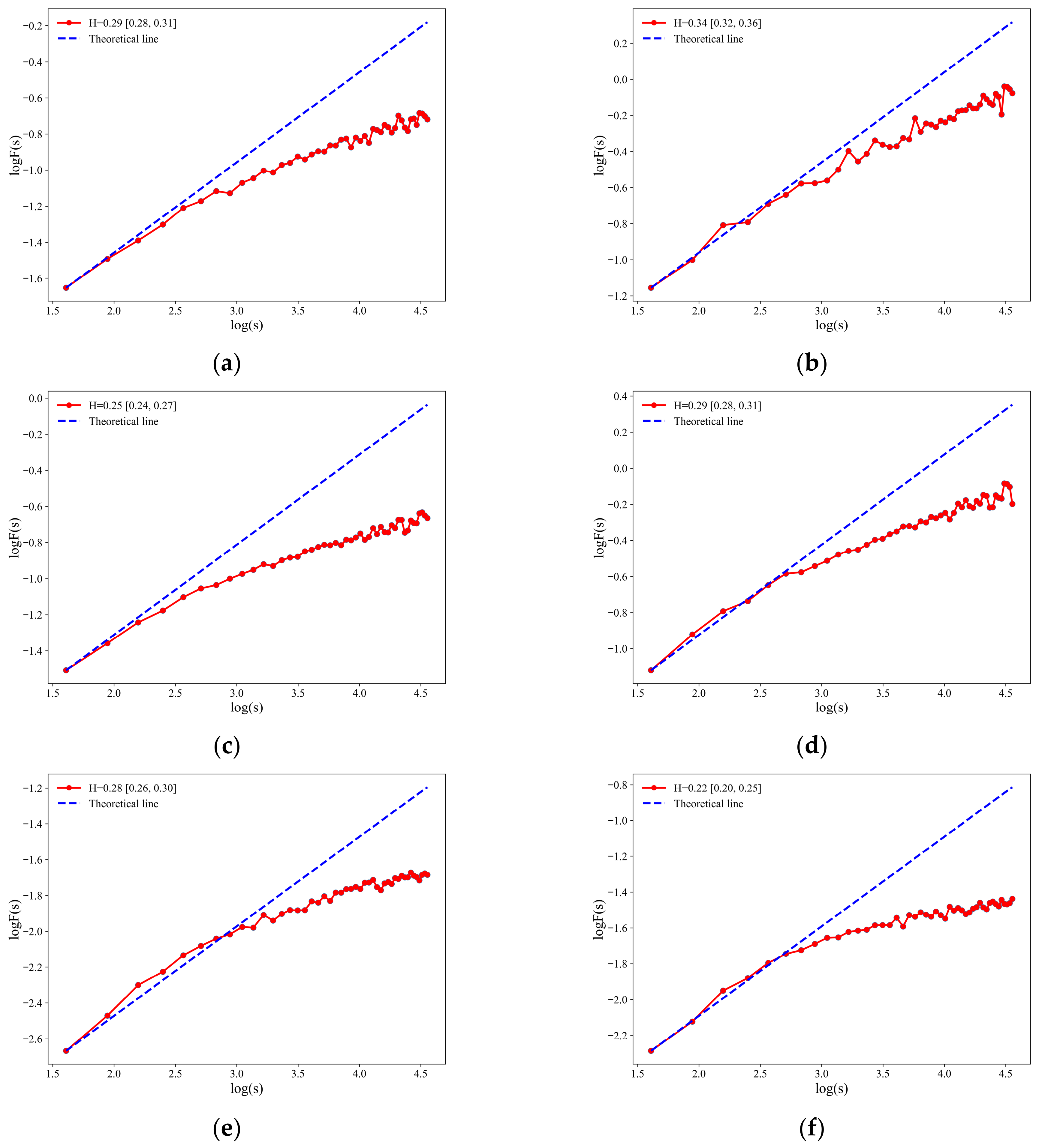
In addition to testing the efficient market hypothesis, this study further applies detrended fluctuation analysis (DFA) to estimate the Hurst exponent of day-ahead and real-time market returns. This allows market efficiency to be evaluated from the perspective of fractal market theory. Based on the method described in Section 2.2.3, the Hurst exponents of day-ahead and real-time returns in Shandong, Shanxi and Guangdong range from 0.22 to 0.34, indicating pronounced anti-persistent behavior. The corresponding 95% confidence intervals are also well below the random-walk benchmark of 0.5. This means that price movements are more likely to reverse than to continue in the same direction, implying short-term mean reversion and a clear deviation from a random walk. Figure 4 presents the log–log plots of $F\left(s\right)$ against $s$ for daily returns in the three provinces, together with the estimated Hurst exponents and their 95% confidence intervals.

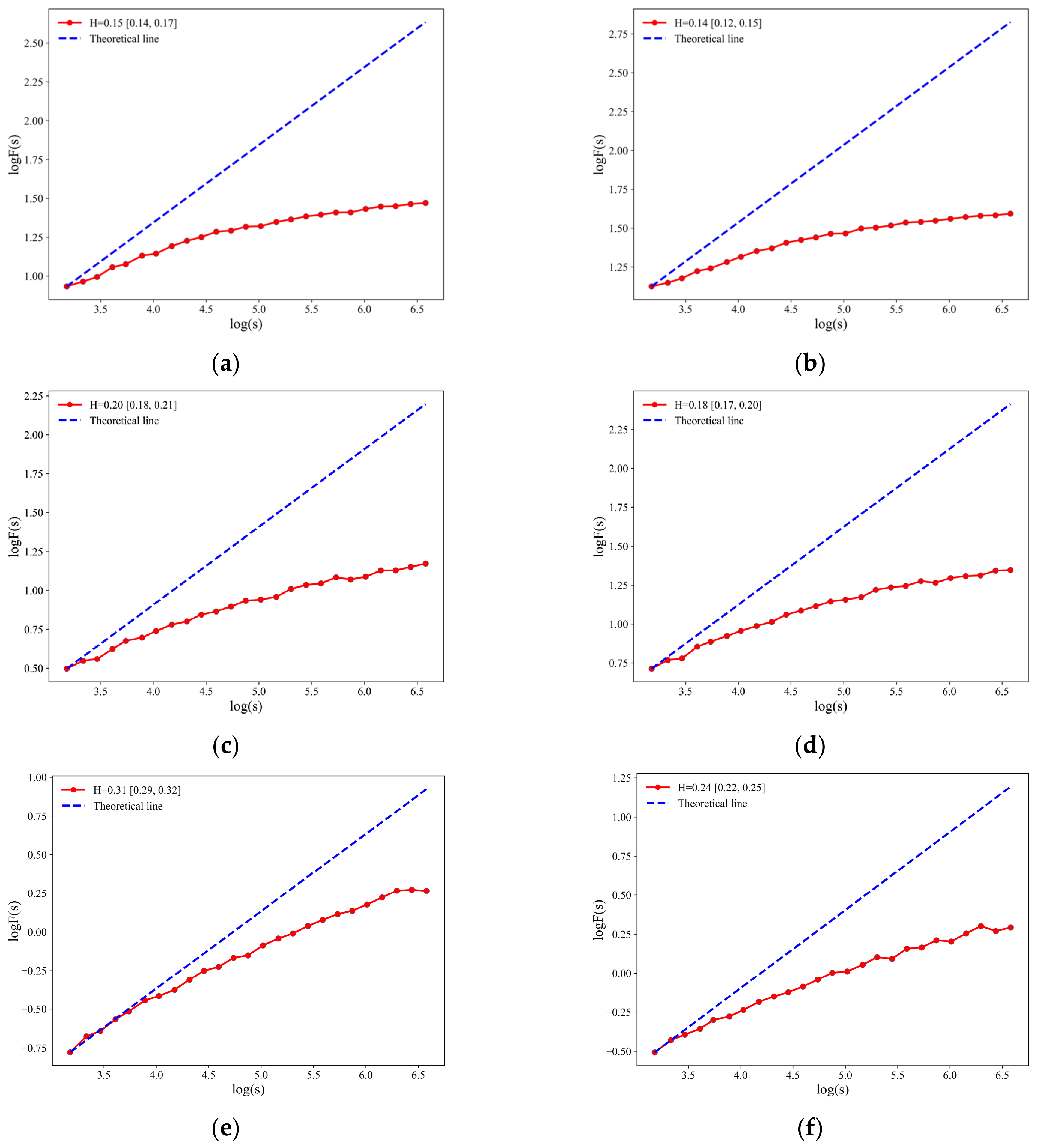
We further conduct DFA using hourly return series. Compared with daily DFA, hourly DFA captures the correlation structure of price fluctuations over a shorter time horizon. The daily results mainly reflect cross-day information absorption and price adjustment, whereas the hourly results are more strongly influenced by intraday load variation and fluctuations in renewable output. As shown in Figure 5, the Hurst exponents of hourly returns in Shandong, Shanxi and Guangdong range from 0.14 to 0.31, again indicating anti-persistence and mean-reverting behavior. Moreover, the hourly results deviate more strongly from the random-walk benchmark than the daily results, suggesting that high-frequency price dynamics are more strongly affected by intraday periodicity, market frictions and short-term noise.

Overall, the DFA results consistently show that the Hurst exponents of both daily and hourly return series are well below 0.5. The estimated Hurst exponents indicate that price returns are not independent across time scales. Instead, the anti-persistent pattern suggests repeated price correction and short-term reversal. This means that market participants with different time horizons may face a price process that still contains systematic dependence, rather than a fully random and informationally efficient process.

Table A8. Robustness test of DFA of daily return.

Province	Market	${\mathit{n}}_{\mathit{m}\mathit{i}\mathit{n}}$	${\mathit{n}}_{\mathit{m}\mathit{a}\mathit{x}}$	Hurst	95% CI
Shandong	DA	8	N/10	0.28	[0.26, 0.29]
Shandong	DA	6	N/12	0.30	[0.29, 0.32]
Shandong	DA	8	N/12	0.28	[0.27, 0.30]
Shandong	RT	8	N/10	0.32	[0.30, 0.33]
Shandong	RT	6	N/12	0.33	[0.31, 0.34]
Shandong	RT	8	N/12	0.32	[0.31, 0.33]
Shanxi	DA	8	N/10	0.23	[0.22, 0.24]
Shanxi	DA	6	N/12	0.24	[0.22, 0.24]
Shanxi	DA	8	N/12	0.23	[0.23, 0.26]
Shanxi	RT	8	N/10	0.27	[0.26, 0.28]
Shanxi	RT	6	N/12	0.29	[0.28, 0.30]
Shanxi	RT	8	N/12	0.27	[0.26, 0.28]
Guangdong	DA	8	N/10	0.25	[0.23, 0.26]
Guangdong	DA	6	N/12	0.27	[0.26, 0.29]
Guangdong	DA	8	N/12	0.26	[0.24, 0.27]
Guangdong	RT	8	N/10	0.18	[0.17, 0.20]
Guangdong	RT	6	N/12	0.21	[0.19, 0.23]
Guangdong	RT	8	N/12	0.19	[0.18, 0.21]

Note: $n_{min}$ and $n_{max}$ denote the minimum and maximum box sizes used in the DFA estimation, respectively and $N$ is the sample size of each return series.

and

Table A9. Robustness test of DFA of hourly return.

Province	Market	${\mathit{n}}_{\mathit{m}\mathit{i}\mathit{n}}$	${\mathit{n}}_{\mathit{m}\mathit{a}\mathit{x}}$	Hurst	95% CI
Shandong	DA	8	N/10	0.26	[0.22, 0.31]
Shandong	DA	6	N/12	0.31	[0.25, 0.36]
Shandong	DA	8	N/12	0.26	[0.22, 0.31]
Shandong	RT	8	N/10	0.24	[0.20, 0.28]
Shandong	RT	6	N/12	0.28	[0.23, 0.33]
Shandong	RT	8	N/12	0.24	[0.20, 0.28]
Shanxi	DA	8	N/10	0.28	[0.24, 0.32]
Shanxi	DA	6	N/12	0.32	[0.28, 0.36]
Shanxi	DA	8	N/12	0.28	[0.24, 0.32]
Shanxi	RT	8	N/10	0.27	[0.23, 0.30]
Shanxi	RT	6	N/12	0.30	[0.26, 0.34]
Shanxi	RT	8	N/12	0.27	[0.23, 0.30]
Guangdong	DA	8	N/10	0.35	[0.33, 0.37]
Guangdong	DA	6	N/12	0.37	[0.35, 0.40]
Guangdong	DA	8	N/12	0.35	[0.33, 0.37]
Guangdong	RT	8	N/10	0.27	[0.26, 0.29]
Guangdong	RT	6	N/12	0.30	[0.28, 0.32]
Guangdong	RT	8	N/12	0.27	[0.26, 0.29]

Note: $n_{min}$ and $n_{max}$ denote the minimum and maximum box sizes used in the DFA estimation, respectively and $N$ is the sample size of each return series.

report the robustness results of the DFA.

3.4. Trends of Market Efficiency

This study further applies the sample entropy method to characterize the time-varying market efficiency in Shandong, Shanxi and Guangdong. The sample entropy values of the electricity spot markets are calculated based on Equation (15) and the results are reported in

Table 9. Sample entropy results of electricity spot markets.

Province	DA Market	RT Market
Shandong	0.505	0.422
Shanxi	0.683	0.555
Guangdong	1.127	1.458

Note: $m=2$, $r=0.2 \ast SD.$

. The entropy results provide another perspective on information efficiency. Higher entropy indicates that price returns contain richer and less predictable patterns, while lower entropy suggests that price movements are more regular and easier to anticipate.

The results show that Guangdong has the highest sample entropy in both the day-ahead and real-time markets, while Shandong records the lowest values. This indicates that Guangdong’s price returns are less regular and less predictable, whereas Shandong’s price dynamics contain more regular patterns. These findings suggest relatively higher information efficiency in Guangdong and relatively lower efficiency in Shandong. Nevertheless, the entropy results do not imply that any of the three markets is fully efficient. Instead, the results show that overall market efficiency remains limited, with clear cross-provincial differences.

Table A10. Robustness test of sample entropy in day-ahead market.

Province	m	r Ratio	Window Size	Sample Entropy
Shandong	2	0.15	180	0.711
Shanxi	2	0.15	180	0.914
Guangdong	2	0.15	180	1.414
Shandong	2	0.25	180	0.394
Shanxi	2	0.25	180	0.629
Guangdong	2	0.25	180	0.979
Shandong	3	0.2	180	0.476
Shanxi	3	0.2	180	0.669
Guangdong	3	0.2	180	1.152
Shandong	2	0.2	90	0.544
Shanxi	2	0.2	90	0.817
Guangdong	2	0.2	90	1.198
Shandong	2	0.2	270	0.506
Shanxi	2	0.2	270	0.689
Guangdong	2	0.2	270	1.119

and

Table A11. Robustness test of sample entropy in real-time market.

Province	m	r Ratio	Window Size	Sample Entropy
Shandong	2	0.15	180	0.622
Shanxi	2	0.15	180	0.871
Guangdong	2	0.15	180	1.762
Shandong	2	0.25	180	0.330
Shanxi	2	0.25	180	0.523
Guangdong	2	0.25	180	1.273
Shandong	3	0.2	180	0.419
Shanxi	3	0.2	180	0.606
Guangdong	3	0.2	180	1.481
Shandong	2	0.2	90	0.483
Shanxi	2	0.2	90	0.710
Guangdong	2	0.2	90	1.564
Shandong	2	0.2	270	0.421
Shanxi	2	0.2	270	0.627
Guangdong	2	0.2	270	1.447

show the results of the robustness tests.

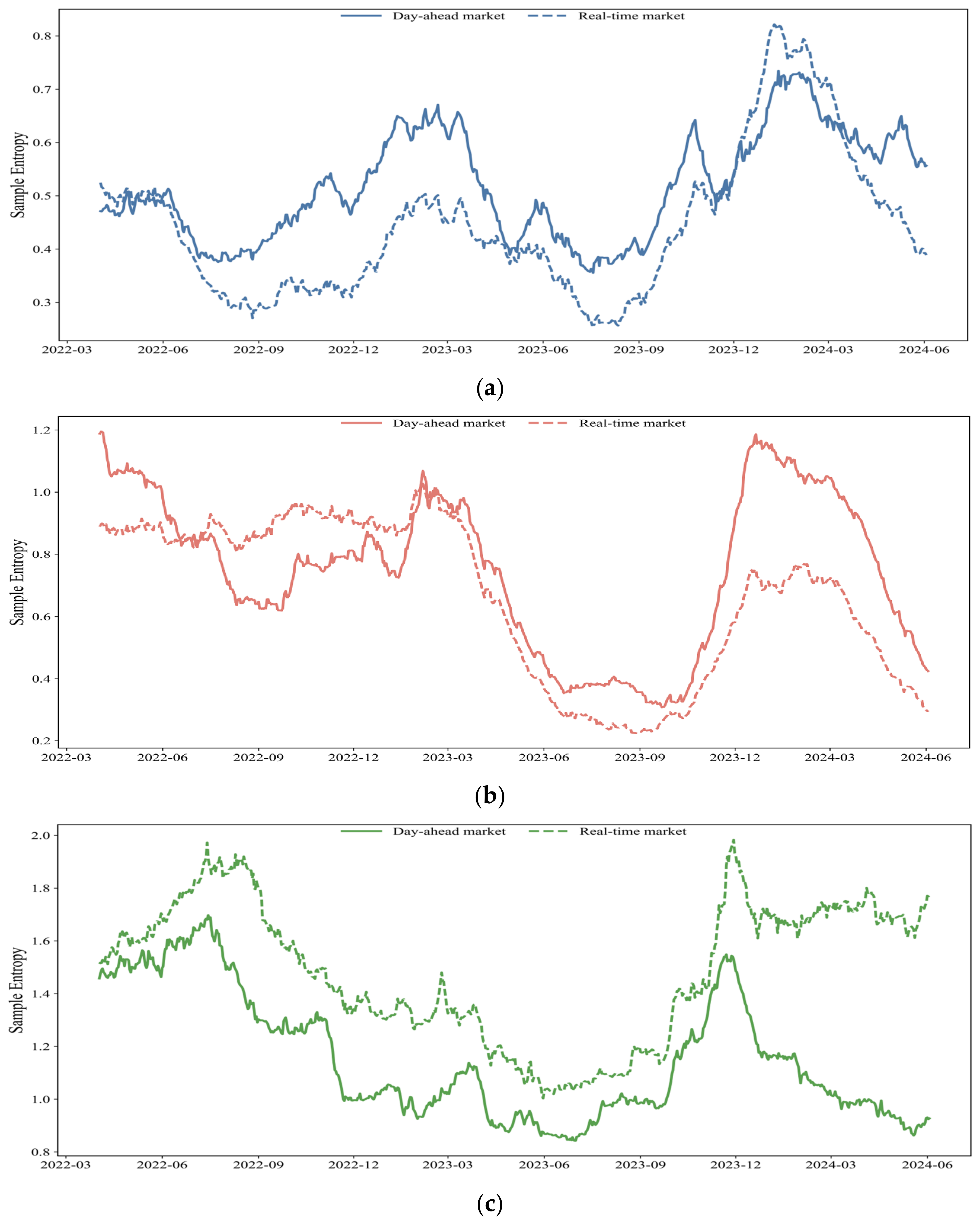
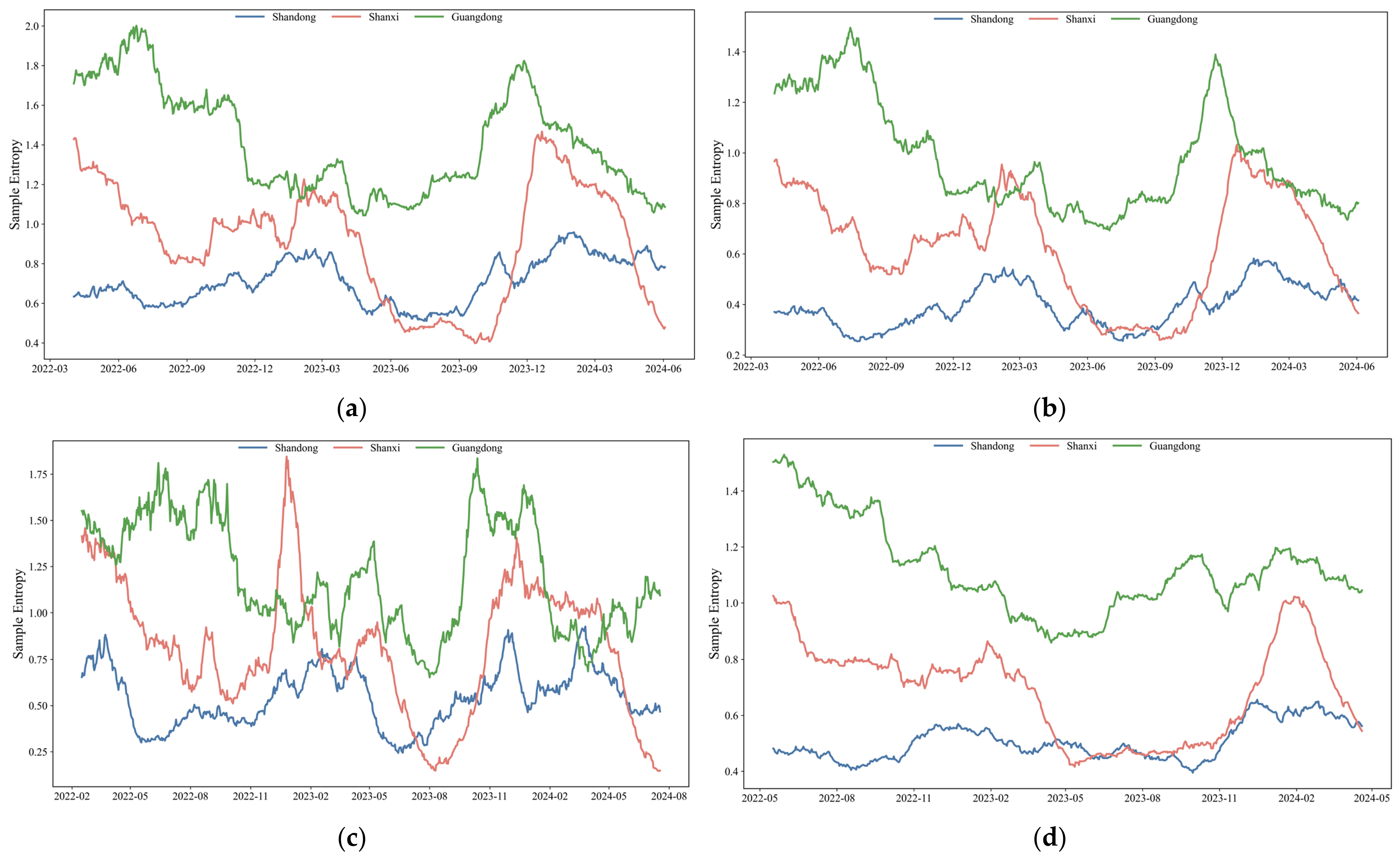
To further examine the time-varying characteristics of price fluctuations, this study applies sample entropy within a sliding window framework to measure the evolution of market efficiency over time. The window length is set to 180 days.

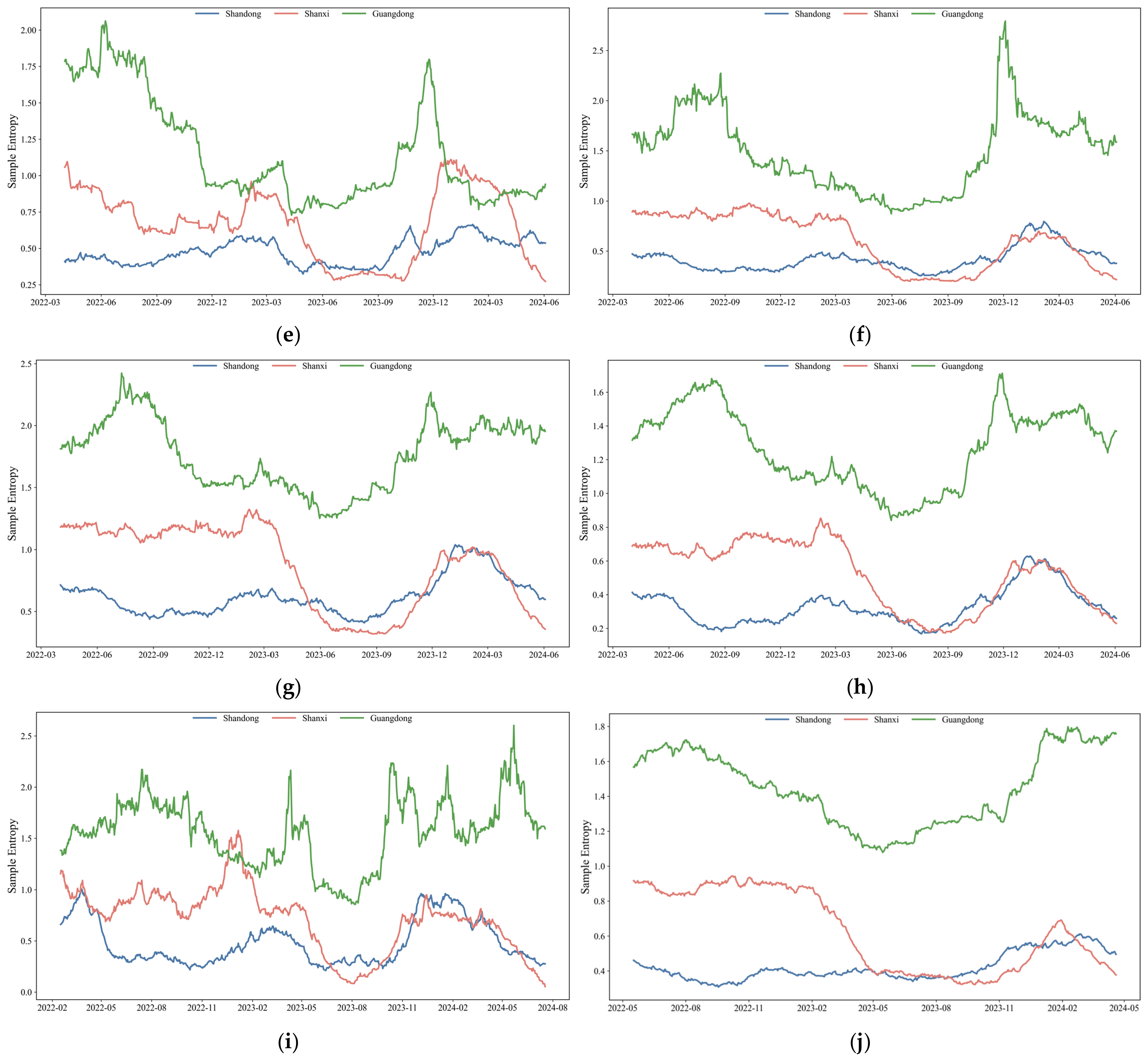
Figure 6 shows the time-varying sample entropy of day-ahead and real-time electricity spot prices in Shandong, Shanxi and Guangdong. By plotting the two market segments together for each province, the figure provides a direct comparison of their efficiency dynamics. The results show that the relationship between day-ahead and real-time entropy differs across provinces and changes over time. In Shandong, the two series do not show a stable dominance pattern. Real-time entropy is higher in some periods, especially in the early sample period and around late 2023 to early 2024, while day-ahead entropy is higher during several other intervals. In Shanxi, real-time entropy is higher before early 2023, but the two series become much closer afterward. In Guangdong, real-time entropy remains above day-ahead entropy for most of the sample period, suggesting that real-time prices contain more complex short-term fluctuations. The differences between the two market segments may reflect the role of short-term information, including demand fluctuations, renewable output variation and balancing conditions, in real-time price formation. Figure A1 reports the robustness results for the trends in electricity spot market efficiency.

3.5. Summary of Empirical Findings

Table 10. Cross-method comparison of market efficiency.

Province	Unit Root		Price Convergence	Hurst		Sample Entropy
	DA	RT	DA&RT	DA	RT	DA	RT
Shandong	4	1	29%	0.29	0.34	0.51	0.42
Shanxi	4	1	33%	0.25	0.29	0.68	0.56
Guangdong	9	5	25%	0.28	0.22	1.13	1.46

Note: The unit root columns report the average annual number of hourly periods for which the null hypothesis of a unit root cannot be rejected. Price convergence is measured as the share of hours for which day-ahead and real-time prices converge. Hurst exponents below 0.5 indicate anti-persistent behavior and higher sample entropy indicates lower predictability and thus higher market efficiency.

provides a cross-method summary of the market efficiency results. The full-sample results are used as the main basis for the overall assessment because they cover a longer period and are less affected by short-term fluctuations in market operation, fuel costs and supply–demand conditions. By contrast, the annual results reported above are useful for showing that market efficiency may change over time, but they are more sensitive to year-specific conditions. Overall, the evidence suggests that none of the three provincial electricity spot markets can be regarded as fully efficient.

The results also show that the relative performance of each province differs across indicators. Guangdong performs relatively better in the unit root and sample entropy results, but it has the lowest day-ahead and real-time price convergence ratio. Shanxi shows the highest price convergence ratio, while its Hurst exponents and entropy values still indicate limited efficiency. These differences should not be viewed as contradictory. Electricity market efficiency involves several related but distinct aspects of price formation. A market may show lower predictability in its own price series, but still exhibit limited consistency between day-ahead and real-time prices. Similarly, stronger price convergence does not necessarily mean that price returns are free from mean reversion or other dependence structures. Therefore, the indicators in Table 10 should be interpreted as complementary evidence on price predictability, inter-market consistency, fractal dependence and information complexity.

Table 10 further indicates that market efficiency differs across the three provincial markets. Overall, Guangdong appears to show relatively higher efficiency, Shandong shows relatively lower efficiency, and Shanxi generally lies between the two. These differences suggest that the efficiency of price formation varies across provincial electricity markets and may be associated with province-specific conditions. The following discussion further relates the observed cross-provincial efficiency differences to intraday load patterns, generation mix and ownership concentration.

4. Discussion

To further interpret the differences in market efficiency, this section discusses the intraday load patterns, generation mix, market structure and market design in the three provincial markets.

4.1. Intraday Load Patterns and Market Efficiency

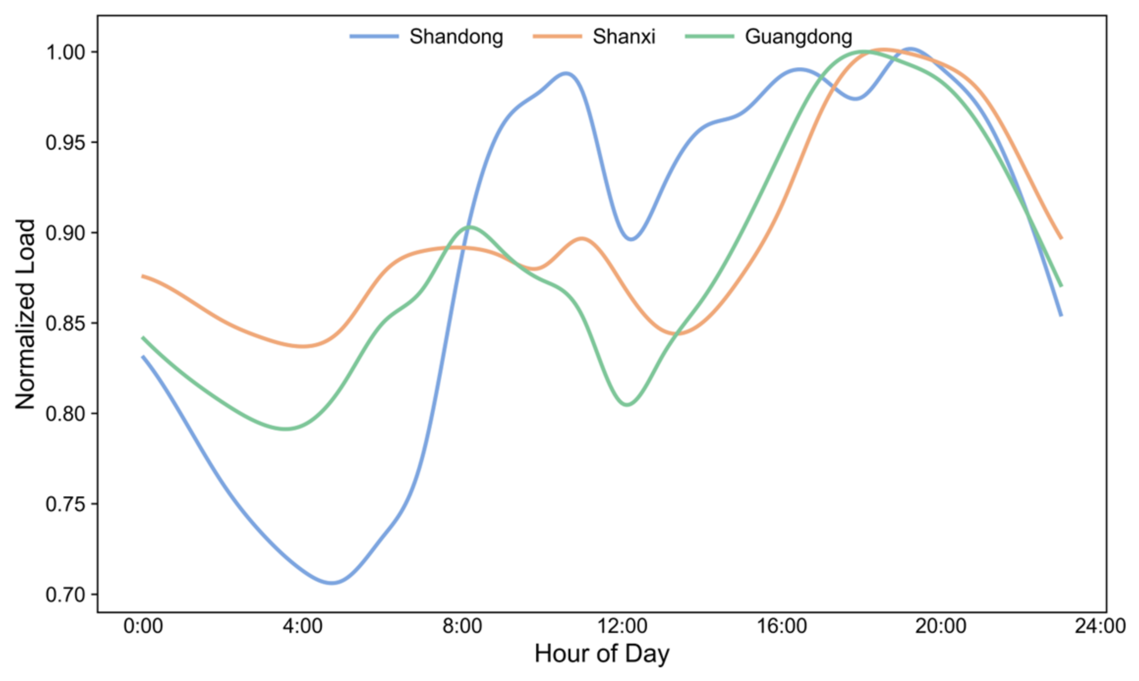
To examine whether demand-side conditions help explain cross-provincial differences in market efficiency, this study compares the normalized average daily load curves of Shandong, Shanxi and Guangdong. The hourly average load of each province is normalized by the maximum value of its own average daily load curve, so that the comparison emphasizes intraday load shape rather than absolute load size. This allows a clearer comparison of peak–valley structure across provinces.

Figure 7 shows noticeable differences in intraday load patterns across the three provinces. Shandong displays a pronounced two-stage pattern, with load rising rapidly in the morning, falling back around midday, and then increasing again toward the evening peak. Shanxi has a relatively smoother profile overall, although its load still increases steadily in the late afternoon and evening. Guangdong exhibits the deepest early-morning valley and a steep rise from the morning to the daytime plateau, followed by another increase toward the evening peak. These patterns suggest that the three provincial systems face different forms of intraday balancing pressure.

These differences may help explain part of the observed variation in market efficiency. More uneven intraday load movements, especially sharp ramps and distinct peak transitions, can increase the difficulty of real-time balancing and make prices more sensitive to short-term scarcity. In this sense, the more volatile intraday profile in Shandong may contribute to less stable price formation. At the same time, Guangdong’s market performs relatively better in the efficiency tests despite also showing substantial intraday variation. One possible explanation is that Guangdong has a larger share of gas-fired generation, which generally offers greater operational flexibility and can respond more quickly to short-term demand changes. This suggests that demand-side load patterns alone cannot fully explain cross-provincial differences in market efficiency. The ability of the market to absorb and respond to such variation through supply flexibility also plays an important role.

As power systems integrate more variable renewable energy, the ability to accommodate steep ramps and intraday fluctuations becomes increasingly important. Efficient markets should translate these system conditions into stable and informative price signals, which are essential for guiding flexible generation, storage and demand response. Therefore, strengthening market design and operational flexibility is an important complement to the low-carbon transition in electricity markets.

4.2. Generation Mix and Market Efficiency

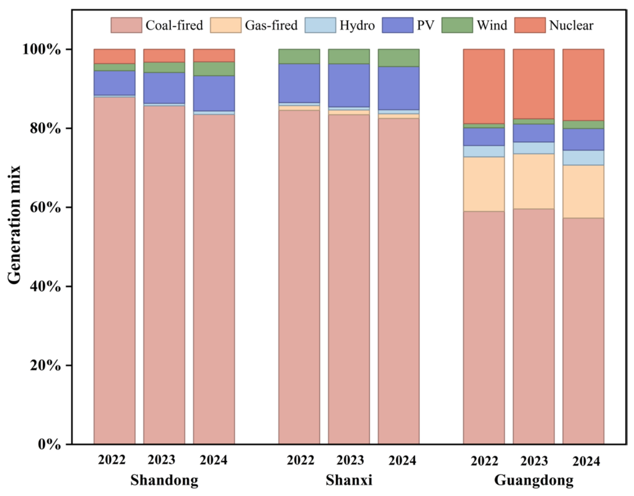
In addition to intraday load patterns, differences in generation mix may also help explain cross-provincial variation in market efficiency. Figure 8 shows that Shandong and Shanxi relied heavily on coal-fired generation during 2022–2024, with coal-fired power consistently accounting for more than 80% of total generation. By contrast, Guangdong exhibited a more diversified generation structure, with a lower share of coal-fired power and higher shares of gas-fired and nuclear generation. Such a generation mix may be associated with different price formation and balancing conditions, because gas-fired units are generally more flexible while nuclear generation provides stable baseload supply. At the same time, the shares of PV and wind generation increased gradually in both Shandong and Shanxi, indicating a growing role of variable renewable energy in these two provincial power systems.

These differences in generation mix are relevant to market efficiency because they shape supply-side flexibility and the cost structure of price formation. The increasing penetration of PV and wind generation may further complicate price formation. Renewable generation has low marginal cost and uncertain output, which can compress prices during high-output periods [6] and increase balancing pressure when output declines [51]. Therefore, higher renewable integration increases the importance of flexible resources and effective short-term price signals. In a system dominated by thermal generation, price adjustment may be less flexible when demand or renewable output changes rapidly within the day. This is because thermal units often face operational constraints under variable operating conditions [52]. By contrast, a more diversified generation mix, especially one with more flexible generation resources, can help the supply side respond more smoothly to changing system conditions [53]. This may reduce predictable price patterns and improve the quality of price signals.

In this sense, generation mix provides a possible perspective for understanding cross-provincial variation in market efficiency. A more diversified generation structure may improve the ability of the power system to absorb demand fluctuations and output variability, while a heavier reliance on thermal generation may be associated with a less flexible adjustment process under changing system conditions. From the perspective of a flexible and low-carbon power system, a more balanced generation mix can contribute to more adaptive system operation and, potentially, to more efficient price formation.

4.3. Market Structure and Market Efficiency

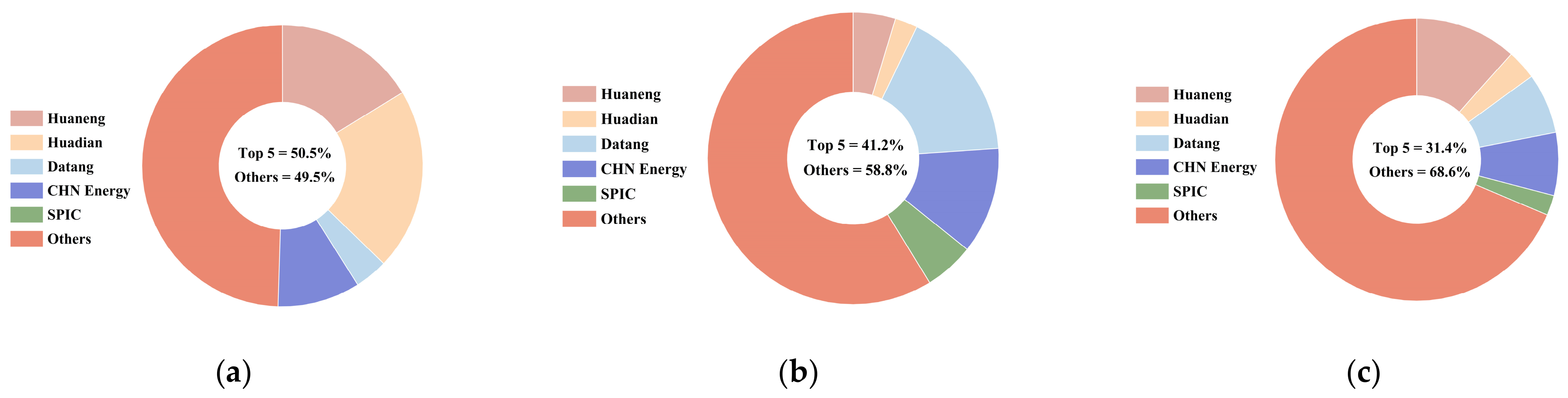
Market efficiency is influenced not only by supply–demand conditions, but also by market structure. In electricity spot markets, the ownership distribution of generation assets affects the intensity of competition. To provide additional context for the efficiency differences observed across provinces, Figure 9 compares the installed-capacity shares of the five major power generation groups in Shandong, Shanxi and Guangdong.

The results show clear cross-provincial differences in market structure. In Shandong, the combined installed-capacity share of the top five generation groups (the top 5 generation groups in China are China Huaneng Group, China Huadian Corporation, China Datang Corporation, China Energy Investment Corporation and State Power Investment Corporation) reaches 50.5%, indicating a relatively high degree of concentration. In Shanxi, the corresponding share is 41.2%, which suggests a moderate level of concentration. Guangdong shows the lowest share, with the top five groups accounting for only 31.4% of total installed capacity, while other market participants account for 68.6%. This implies that Guangdong has a more diversified ownership structure on the generation side.

Ownership concentration can affect market efficiency by changing competitive pressure in the bidding process [54]. When a large share of generation capacity is controlled by a small number of firms, competitive pressure may be weaker and market outcomes may become more susceptible to the strategic behavior of large participants [55]. Under such conditions, clearing prices may deviate more easily from short-run marginal system conditions, which can reduce the informational content of market prices. By contrast, a more dispersed ownership structure can strengthen competition among generators and make clearing prices more responsive to changes in demand, fuel costs and renewable output. From this perspective, market structure provides a possible explanation for part of the observed variation in market efficiency across provinces. The higher ownership concentration in Shandong may contribute to less competitive price formation, while Guangdong’s more diversified ownership structure may help explain its relatively better market efficiency. A more competitive market structure can therefore improve the quality of price signals, which is important for the efficient coordination of flexible resources and the integration of low-carbon energy.

4.4. Market Design and Market Efficiency

Market design could also be an important institutional source of market inefficiency. China’s power market reform has made substantial progress, but the construction of provincial electricity spot markets is still characterized by pilot-based development and gradual rule refinement [56]. Existing studies also suggest that China’s electricity market creation is shaped by political–economic and institutional constraints, including the need to coordinate market competition with system security, regulatory oversight and regional interests [57]. In this context, price formation may not fully reflect all available information on demand, fuel costs, renewable output and system scarcity. The coordination between day-ahead and real-time markets is still evolving, which may weaken the convergence between forward scheduling and real-time balancing. In addition, mechanisms related to imbalance settlement, ancillary services and interprovincial trading are still being developed and coordinated within China’s evolving power-market framework [27]. Recent international studies further show that market-design arrangements can shape the strategic behavior of market participants, including strategic bidding by variable renewable generators and operating strategies adopted by prosumers in local electricity markets [58,59]. These institutional features may weaken the transmission of short-term system conditions into market prices, and their effects may differ across provinces depending on local demand patterns, generation mix and supply-side flexibility. Therefore, market design should be viewed not only as a common reform background, but also as a mechanism that may amplify or mitigate provincial differences in market efficiency.

Price regulation may further affect market efficiency. In the three provincial spot markets examined in this study, market-clearing prices are subject to explicit upper and lower bounds. Evidence from Guangdong’s spot-market pilot shows that the price floor caused measurable market distortion and generated a welfare transfer from consumers to generators [60]. These price limits can play a stabilizing role during the early stage of market reform, because they help prevent excessive price spikes and protect market participants from extreme outcomes. However, they may also weaken the informational content of prices. When prices approach the upper bound, scarcity conditions may not be fully reflected in market-clearing prices [7]. When prices approach the lower bound, excess supply or high renewable output may also be only partially reflected. In both cases, price movements are constrained by regulatory rules rather than determined solely by supply and demand fundamentals. Therefore, price regulation may affect market efficiency both as a general institutional constraint and as a factor that interacts with local supply–demand conditions.

5. Conclusions

This study evaluates the efficiency of China’s provincial electricity spot markets using Shandong, Shanxi and Guangdong as representative cases. The results show that none of the provincial spot markets satisfies weak-form efficiency. Most hourly price series are stationary, indicating that electricity prices remain predictable to some extent. The convergence test also reveals limited consistency between day-ahead and real-time prices, with the shares of convergent hours being only 29%, 33% and 25% in Shandong, Shanxi and Guangdong. Moreover, the Hurst exponents of both daily and hourly return series are significantly below 0.5, indicating anti-persistent and mean-reverting behavior rather than a random walk. Taken together, these findings suggest that market information is not yet fully and efficiently incorporated into spot prices.

The discussion suggests that these differences are partly associated with cross-provincial variation in demand conditions, generation characteristics, market structure and institutional design. Shandong exhibits relatively more pronounced intraday load transitions, which may increase balancing difficulty and make prices more sensitive to short-term scarcity. Guangdong shows a more diversified generation mix and a less concentrated ownership structure, which may support smoother price formation and relatively better market efficiency. Institutional factors, including evolving market rules and regulatory price limits, may further influence the extent to which market-clearing prices reflect short-term system conditions. These factors provide potential explanations for the observed cross-provincial differences in market efficiency.

From a policy perspective, improving market efficiency requires better price formation mechanisms and stronger coordination between the day-ahead and real-time markets. It also requires greater operational flexibility and market arrangements that can better absorb demand fluctuations and renewable output variation. More efficient and informative prices can better support flexible generation, storage and demand response and thereby improve the efficient integration of low-carbon energy. Therefore, strengthening market design and operational flexibility, while promoting a more balanced generation mix and a more competitive market structure, is important for both market efficiency and sustainability. In practical terms, the framework used in this study may serve as a useful reference for regulators and market operators to monitor price predictability and assess day-ahead and real-time market coordination. It may also be further applied to track market performance across regions and over time. In addition, the Chinese case also provides useful lessons for other regions undergoing electricity market reforms. The comparisons of Shandong, Shanxi and Guangdong show that regional markets may exhibit different efficiency levels even under a broadly similar reform framework. This suggests that market design should be adapted to local generation structures, demand patterns, renewable integration conditions and regulatory constraints, rather than relying only on uniform institutional arrangements.

Due to data availability constraints, this study has several limitations. First, it cannot explicitly model interregional power flows, transmission constraints or neighboring-market interactions, which may affect residual demand and real-time balancing conditions. Second, although this study identifies temporal changes in market efficiency, it cannot fully distinguish their underlying drivers. Future research could incorporate bidding behavior, unit-level operating constraints and a broader set of provincial markets to better evaluate and explain market efficiency in different regions.

References

1. Erdogdu, E. Implications of Liberalization Policies on Government Support to R&D: Lessons from Electricity Markets. Renew. Sustain. Energy Rev. 2013, 17, 110–118. [Google Scholar] [CrossRef]
2. Morales, L.; Hanly, J. European Power Markets—A Journey towards Efficiency. Energy Policy 2018, 116, 78–85. [Google Scholar] [CrossRef]
3. Xu, C.; Wen, F.; Palu, I. Electricity Market Regulation: Global Status, Development Trend, and Prospect in China. Energy Convers. Econ. 2020, 1, 151–170. [Google Scholar] [CrossRef]
4. Karahan, C.C.; Odabaşı, A.; Tiryaki, C.S. Wired Together: Integration and Efficiency in European Electricity Markets. Energy Econ. 2024, 133, 107505. [Google Scholar] [CrossRef]
5. Rasheed, M.Q.; Yuhuan, Z.; Ahmed, Z. Can Enhancing Competitive Industrial Performance and Adopting Renewables Stimulate Progress toward Carbon Neutrality Targets? Evidence from Asian Developing Countries. Energy Environ. 2025, 0958305X251389830. [Google Scholar] [CrossRef]
6. Hirth, L. The Market Value of Variable Renewables: The Effect of Solar Wind Power Variability on Their Relative Price. Energy Econ. 2013, 38, 218–236. [Google Scholar] [CrossRef]
7. Zhou, Z.; Botterud, A.; Levin, T. Price Formation in Zero-Carbon Electricity Markets—Fundamentals, Challenges, and Research Needs. Renew. Sustain. Energy Rev. 2025, 211, 115250. [Google Scholar] [CrossRef]
8. Kühnlenz, F.; Nardelli, P.H.J.; Karhinen, S.; Svento, R. Implementing Flexible Demand: Real-Time Price vs. Market Integration. Energy 2018, 149, 550–565. [Google Scholar] [CrossRef]
9. Ambec, S.; Crampes, C. Real-Time Electricity Pricing to Balance Green Energy Intermittency. Energy Econ. 2021, 94, 105074. [Google Scholar] [CrossRef]
10. Marshall, L.; Bruce, A.; MacGill, I. Assessing Wholesale Competition in the Australian National Electricity Market. Energy Policy 2021, 149, 112066. [Google Scholar] [CrossRef]
11. Lu, Z.; Dong, Z.; Sanderson, P. The Efficient Market Hypothesis and Electricity Market Efficiency Test. In Proceedings of the 2005 IEEE/PES Transmission & Distribution Conference & Exposition: Asia and Pacific, Dalian, China, 18 August 2005; pp. 1–7. [Google Scholar]
12. Arciniegas, I.; Barrett, C.; Marathe, A. Assessing the Efficiency of US Electricity Markets. Util. Policy 2003, 11, 75–86. [Google Scholar] [CrossRef]
13. Filipiak, I.; Filipiak, P. Efficient Market Hypothesis and Polish Electricity Market. In Proceedings of the 2018 15th International Conference on the European Energy Market (EEM), Lodz, Poland, 27–29 June 2018; pp. 1–5. [Google Scholar]
14. Khan, I. Efficiency Analysis and A Random Forest Based Trading Strategy for Heteroscedastic Electricity Market Data. In Proceedings of the 2022 IEEE Power & Energy Society General Meeting (PESGM), Denver, CO, USA, 17–21 July 2022; pp. 1–5. [Google Scholar]
15. Hirsch, S.; Ziel, F. Simulation-Based Forecasting for Intraday Power Markets: Modelling Fundamental Drivers for Location, Shape and Scale of the Price Distribution. Energy J. 2024, 45, 87–124. [Google Scholar] [CrossRef]
16. Nickelsen, D.; Müller, G. Bayesian Hierarchical Probabilistic Forecasting of Intraday Electricity Prices. Appl. Energy 2025, 380, 124975. [Google Scholar] [CrossRef]
17. Asan, G.; Tasaltin, K. Market Efficiency Assessment under Dual Pricing Rule for the Turkish Wholesale Electricity Market. Energy Policy 2017, 107, 109–118. [Google Scholar] [CrossRef]
18. Castro, A.L.; Marcato, A.L.M.; De Aguiar, E.P. Multifractal Analysis of the Brazilian Electricity Market. IEEE Access 2023, 11, 98939–98957. [Google Scholar] [CrossRef]
19. Ali, H.; Aslam, F.; Ferreira, P. Modeling Dynamic Multifractal Efficiency of US Electricity Market. Energies 2021, 14, 6145. [Google Scholar] [CrossRef]
20. Papaioannou, G.P.; Dikaiakos, C.; Stratigakos, A.C.; Papageorgiou, P.C.; Krommydas, K.F. Testing the Efficiency of Electricity Markets Using a New Composite Measure Based on Nonlinear TS Tools. Energies 2019, 12, 618. [Google Scholar] [CrossRef]
21. Čurpek, J. Time Evolution of Hurst Exponent: Czech Wholesale Electricity Market Study. Eur. Financ. Account. J. 2019, 14, 25–44. [Google Scholar] [CrossRef]
22. Gorjão, L.R.; Witthaut, D.; Lind, P.G.; Medjroubi, W. Change of Persistence in European Electricity Spot Prices. arXiv 2021, arXiv:2112.03513. [Google Scholar] [CrossRef]
23. Ock, S.E.; Lee, M.; Song, J.W. Multifractal Analysis of the Impact of Fuel Cell Introduction in the Korean Electricity Market. Fractal Fract. 2024, 8, 573. [Google Scholar] [CrossRef]
24. Wang, J.; Wang, S. The Effect of Electricity Market Reform on Energy Efficiency in China. Energy Policy 2023, 181, 113722. [Google Scholar] [CrossRef]
25. Cheng, X.; Liu, P.; Zhu, L. The Impact of Electricity Market Reform on Renewable Energy Production. Energy Policy 2024, 194, 114306. [Google Scholar] [CrossRef]
26. Lin, J.; Kahrl, F.; Yuan, J.; Chen, Q.; Liu, X. Economic and Carbon Emission Impacts of Electricity Market Transition in China: A Case Study of Guangdong Province. Appl. Energy 2019, 238, 1093–1107. [Google Scholar] [CrossRef]
27. Guo, H.; Davidson, M.R.; Chen, Q.; Zhang, D.; Jiang, N.; Xia, Q.; Kang, C.; Zhang, X. Power Market Reform in China: Motivations, Progress, and Recommendations. Energy Policy 2020, 145, 111717. [Google Scholar] [CrossRef]
28. Bower, J.; Bunn, D.W. Model-Based Comparisons of Pool and Bilateral Markets for Electricity. Energy J. 2000, 21, 1–29. [Google Scholar] [CrossRef]
29. Zhou, Y.; Shi, Z.; Wu, L. Green Policy under the Competitive Electricity Market: An Agent-Based Model Simulation in Shanghai. J. Environ. Manag. 2021, 299, 113501. [Google Scholar] [CrossRef]
30. Aliabadi, D.E.; Kaya, M.; Şahin, G. An Agent-Based Simulation of Power Generation Company Behavior in Electricity Markets under Different Market-Clearing Mechanisms. Energy Policy 2017, 100, 191–205. [Google Scholar] [CrossRef]
31. Krishnamurthy, D.; Uckun, C.; Zhou, Z.; Thimmapuram, P.R.; Botterud, A. Energy Storage Arbitrage Under Day-Ahead and Real-Time Price Uncertainty. IEEE Trans. Power Syst. 2018, 33, 84–93. [Google Scholar] [CrossRef]
32. Fama, E.F. Efficient Capital Markets: A Review of Theory and Empirical Work. J. Financ. 1970, 25, 383–417. [Google Scholar] [CrossRef]
33. Li, R.; Svoboda, A.J.; Oren, S.S. Efficiency Impact of Convergence Bidding in the California Electricity Market. J. Regul. Econ. 2015, 48, 245–284. [Google Scholar] [CrossRef]
34. Liu, X.; Zhou, X.; Zhu, B.; He, K.; Wang, P. Measuring the Maturity of Carbon Market in China: An Entropy-Based TOPSIS Approach. J. Clean. Prod. 2019, 229, 94–103. [Google Scholar] [CrossRef]
35. Zou, S.; Zhong, T. Multifractal Detrended Cross-Correlation Analysis of the Relation between Price and Volume in European Carbon Futures Markets. Phys. A Stat. Mech. Its Appl. 2020, 537, 122310. [Google Scholar] [CrossRef]
36. Peters, E.E. Fractal Market Analysis: Applying Chaos Theory to Investment and Economics; John Wiley & Sons: Hoboken, NJ, USA, 1994. [Google Scholar]
37. Deng, S.; Inekwe, J.; Smirnov, V.; Wait, A.; Wang, C. Seasonality in Deep Learning Forecasts of Electricity Imbalance Prices. Energy Econ. 2024, 137, 107770. [Google Scholar] [CrossRef]
38. Stefenon, S.F.; Seman, L.O.; Mariani, V.C.; Coelho, L.D.S. Aggregating Prophet and Seasonal Trend Decomposition for Time Series Forecasting of Italian Electricity Spot Prices. Energies 2023, 16, 1371. [Google Scholar] [CrossRef]
39. Stanković, Z.Z.; Rajic, M.N.; Božić, Z.; Milosavljević, P.; Păcurar, A.; Borzan, C.; Păcurar, R.; Sabău, E. The Volatility Dynamics of Prices in the European Power Markets during the COVID-19 Pandemic Period. Sustainability 2024, 16, 2426. [Google Scholar] [CrossRef]
40. Ganepola, C.N.; Shubita, M.; Lee, L. The Electric Shock: Causes and Consequences of Electricity Prices in the United Kingdom. Energy Econ. 2023, 126, 107030. [Google Scholar] [CrossRef]
41. Li, J.; Li, Y.; Liu, H.-L.; Li, X.-X.; Yu, G.-M.; Yuan, R.-J.; Li, Y.; Hu, Y.-Y.; Zheng, X.-M. Analysis on the Correlation Characteristics of Electricity Trading Price Based on Multifractal Theory. In Proceedings of the 2022 IEEE 6th Conference on Energy Internet and Energy System Integration (EI2), Chengdu, China, 11–13 November 2022; pp. 2809–2814. [Google Scholar]
42. Alvarez-Ramirez, J.; Escarela-Perez, R. Time-Dependent Correlations in Electricity Markets. Energy Econ. 2010, 32, 269–277. [Google Scholar] [CrossRef]
43. Fan, J.-L.; Tang, B.-J.; Yu, H.; Hou, Y.-B.; Wei, Y.-M. Impact of Climatic Factors on Monthly Electricity Consumption of China’s Sectors. Nat. Hazards 2015, 75, 2027–2037. [Google Scholar] [CrossRef]
44. Dickey, D.A.; Fuller, W.A. Distribution of the Estimators for Autoregressive Time Series with a Unit Root. J. Am. Stat. Assoc. 1979, 74, 427–431. [Google Scholar] [CrossRef]
45. Liu, X.; Zhou, X.; Zhu, B.; Wang, P. Measuring the Efficiency of China’s Carbon Market: A Comparison between Efficient and Fractal Market Hypotheses. J. Clean. Prod. 2020, 271, 122885. [Google Scholar] [CrossRef]
46. Phinyomark, A.; Larracy, R.; Scheme, E. Fractal Analysis of Human Gait Variability via Stride Interval Time Series. Front. Physiol. 2020, 11, 333. [Google Scholar] [CrossRef] [PubMed]
47. Gulko, L. The Entropy Theory of Stock Option Pricing. Int. J. Theor. Appl. Financ. 1999, 02, 331–355. [Google Scholar] [CrossRef]
48. Delgado-Bonal, A.; Marshak, A. Approximate Entropy and Sample Entropy: A Comprehensive Tutorial. Entropy 2019, 21, 541. [Google Scholar] [CrossRef]
49. Shimomura, M.; Keeley, A.R.; Matsumoto, K.; Tanaka, K.; Managi, S. Beyond the Merit Order Effect: Impact of the Rapid Expansion of Renewable Energy on Electricity Market Price. Renew. Sustain. Energy Rev. 2024, 189, 114037. [Google Scholar] [CrossRef]
50. Borenstein, S.; Bushnell, J.B.; Wolak, F.A. Measuring Market Inefficiencies in California’s Restructured Wholesale Electricity Market. Am. Econ. Rev. 2002, 92, 1376–1405. [Google Scholar] [CrossRef]
51. Shahzad, S.; Jasińska, E. Renewable Revolution: A Review of Strategic Flexibility in Future Power Systems. Sustainability 2024, 16, 5454. [Google Scholar] [CrossRef]
52. Yuan, R.; Liu, M.; Chen, W.; Yan, J. Costs versus Revenues of Flexibility Enhancement Techniques for Thermal Power Units in Electricity-Carbon Joint Markets. Energy 2024, 302, 131925. [Google Scholar] [CrossRef]
53. Rahman, M.M.; Dadon, S.H.; He, M.; Giesselmann, M.; Hasan, M.M. An Overview of Power System Flexibility: High Renewable Energy Penetration Scenarios. Energies 2024, 17, 6393. [Google Scholar] [CrossRef]
54. Lundin, E.; Tangerås, T.P. Cournot Competition in Wholesale Electricity Markets: The Nordic Power Exchange, Nord Pool. Int. J. Ind. Organ. 2020, 68, 102536. [Google Scholar] [CrossRef]
55. Weber, C.; Möst, D.; Fichtner, W. Imperfect Competition and Market Power. In Economics of Power Systems: Fundamentals for Sustainable Energy; Weber, C., Möst, D., Fichtner, W., Eds.; Springer International Publishing: Cham, Switzerland, 2022; pp. 293–313. [Google Scholar]
56. Feng, Y.; Lin, J.; Song, F.; Ho, M.S. Performance and Challenges of Power Sector Reform in China since 2015. iScience 2025, 28, 113461. [Google Scholar] [CrossRef]
57. Lei, N.; Chen, L.; Sun, C.; Tao, Y. Electricity Market Creation in China: Policy Options from Political Economics Perspective. Sustainability 2018, 10, 1481. [Google Scholar] [CrossRef]
58. Sousa, V.; Algarvio, H. Strategic Bidding to Increase the Market Value of Variable Renewable Generators in Electricity Markets. Energies 2025, 18, 1586. [Google Scholar] [CrossRef]
59. Mochi, P.; Pandya, K.S.; Faia, R.; Dabhi, D.; Soares, J.; Vale, Z. Empowering Customers in Local Electricity Market: A Prosumer Segmentation and Operating Envelope Strategy for Joint Cost Reduction and Profit Maximization. Electr. Power Syst. Res. 2024, 226, 109908. [Google Scholar] [CrossRef]
60. Liu, Y.; Jiang, Z.; Guo, B. Assessing China’s Provincial Electricity Spot Market Pilot Operations: Lessons from Guangdong Province. Energy Policy 2022, 164, 112917. [Google Scholar] [CrossRef]
Figure 1. Merit-order clearing mechanism in a pool-based electricity spot market.
Sustainability 18 04960 g001
Figure 2. Analytical framework for assessing electricity market efficiency.
Sustainability 18 04960 g002
Figure 3. Intraday patterns of hourly electricity prices: (a) Shandong; (b) Shanxi; (c) Guangdong.
Sustainability 18 04960 g003
Figure 4. Log–log plots of F ( s ) against s for daily returns: (a) Shandong day-ahead market; (b) Shandong real-time market; (c) Shanxi day-ahead market; (d) Shanxi real-time market; (e) Guangdong day-ahead market; (f) Guangdong real-time market.
Sustainability 18 04960 g004
Figure 5. Log–log plots of F ( s ) against s for hourly returns: (a) Shandong day-ahead market; (b) Shandong real-time market; (c) Shanxi day-ahead market; (d) Shanxi real-time market; (e) Guangdong day-ahead market; (f) Guangdong real-time market.
Sustainability 18 04960 g005
Figure 6. Trends in electricity spot market efficiency: (a) Shandong; (b) Shanxi; (c) Guangdong.
Sustainability 18 04960 g006
Figure 7. Normalized average daily load curves of Shandong, Shanxi and Guangdong.
Sustainability 18 04960 g007
Figure 8. Generation mix in Shandong, Shanxi and Guangdong.
Sustainability 18 04960 g008
Figure 9. Ownership structure of generation capacity: (a) Shandong; (b) Shanxi; (c) Guangdong.
Sustainability 18 04960 g009