


Abstract
Saline water intrusion poses a major threat to groundwater security in arid and semi-arid regions, reducing freshwater availability and challenging sustainable water resource management. Accurate delineation of the fresh-saline water interface is therefore essential; however, conventional hydrochemical and laboratory-based assessments remain costly, invasive, and spatially limited. Resistivity methods have long been used to infer subsurface salinity, as low resistivity typically reflects clay-rich saline water and higher resistivity reflects freshwater-bearing sand or gravel. Yet, resistivity values for similar lithologies frequently overlap, causing ambiguity in distinguishing fresh and saline aquifers. To overcome this limitation, Dar–Zarrouk (D–Z) parameters are often applied to enhance hydrogeophysical discrimination, but previous studies have relied exclusively on one-dimensional (1D) D–Z derivations using vertical electrical sounding (VES), which cannot resolve the lateral complexity of alluvial aquifers. This study presents the first application of electrical resistivity tomography (ERT) to derive two- and three-dimensional D–Z parameters for detailed mapping of the fresh-saline water interface in the alluvial aquifers of Punjab, Pakistan. ERT provides non-invasive, continuous, and high-resolution subsurface imaging, enabling volumetric assessment of aquifer electrical properties and salinity structure. The resulting 2D/3D models reveal the geometry, depth, and spatial continuity of salinity transitions with far greater clarity than VES-based or purely hydrochemical methods. Physicochemical analyses from boreholes along the ERT profiles independently verify the geophysical interpretations. The findings demonstrate that ERT-derived 2D/3D D–Z modeling offers a cost-effective, scalable, and significantly more accurate framework for assessing fresh-saline water boundaries. This approach provides a transformative pathway for sustainable groundwater monitoring, improved well siting, and long-term aquifer protection in salinity-stressed alluvial regions.
1. Introduction
Groundwater is the primary source of freshwater for domestic, agricultural and industrial needs in many arid and semi-arid regions of the world. In South Asia, and particularly in Pakistan, groundwater plays an indispensable role in sustaining the population and economy due to the limited and highly variable nature of surface water resources [1]. Although only about 0.69% of global water is directly available for human use [2], groundwater constitutes the major share of this accessible freshwater, stored within alluvial and hard rock aquifers through the infiltration of rainfall, river seepage and irrigation return flows [3,4]. Historically, surface water dominated irrigation and supply, but rapid population growth, climate variability and expansion of irrigated agriculture have shifted the burden increasingly toward groundwater abstraction [5,6].
In Pakistan’s Indus Basin—home to nearly 90% of the country’s population—groundwater extraction has intensified sharply over recent decades [7,8]. About 31 million ha of irrigated land already depends on the Indus Basin irrigation system [9], and more than 0.8 million tube wells operate in Punjab alone [10]. The Upper Indus Basin, including the districts of Lahore and Kasur in the Lower Bari Doab, is characterized by dense agricultural development supported by a vast network of private and public tube wells [11]. The uncontrolled proliferation of these wells, often installed without prior geotechnical or geophysical investigation, has led to massive exploitation of groundwater, progressive lowering of water levels and widespread salinization [12,13,14,15].
Excessive abstraction, combined with insufficient natural recharge, disrupts the hydraulic balance between fresh and saline groundwater. As freshwater heads decline, deeper saline water migrates upward and laterally, intruding into previously fresh zones and degrading water quality [16,17]. These processes are well documented in many parts of the Upper and Lower Indus Basin, where increasing groundwater demand, reduced river flows and high evapotranspiration have intensified salinity hazards [18,19,20]. Kasur District, located between the Ravi and Sutlej rivers, is particularly affected: its alluvial aquifer exhibits strong vertical and lateral salinity contrasts, with shallow freshwater lenses overlying brackish to saline groundwater at depth. Under such conditions, accurate delineation of the fresh-saline water interface is critical for sustainable groundwater management, well siting and the protection of groundwater-dependent communities.
Traditionally, the assessment of salinity intrusion relies on borehole drilling, hydrochemical sampling and laboratory analysis. While effective locally, these methods are expensive, intrusive, time-consuming and spatially sparse, and therefore impractical for regional-scale mapping in heterogeneous aquifer systems [21,22]. Surface geophysical techniques, particularly electrical resistivity methods, offer efficient non-invasive alternatives for characterizing subsurface salinity distributions [1,23,24,25]. Vertical electrical sounding (VES) has long been used to infer the depth and extent of fresh-saline aquifers based on resistivity contrasts, as freshwater-bearing sands and gravels typically exhibit higher resistivity than clay-rich or saline-saturated zones [1,22,26,27,28,29]. However, resistivity alone often suffers from ambiguity: similar resistivity ranges can be observed for different combinations of lithology and pore-water salinity, leading to intermixing of signatures for clays, brackish and saline aquifers and clean sand layers [4,30,31]. This problem is particularly acute in the alluvial plains of the Indus Basin, where complex arrangements of clay lenses, silt bands and sand bodies generate highly heterogeneous geoelectrical responses [19,22].
To reduce these ambiguities, Dar–Zarrouk (D–Z) parameters—longitudinal conductance, transverse resistance and longitudinal resistivity—have been widely used to improve the discrimination between fresh, brackish and saline aquifers [19,32,33,34]. These parameters integrate layer resistivity and thickness, providing a more robust representation of hydrostratigraphic properties than resistivity alone and allowing clearer demarcation of fresh-saline boundaries [1,35]. Numerous studies have successfully applied D–Z parameters computed from VES data to delineate the fresh-saline interface in alluvial and coastal aquifers [1,4,19,22,26,27,29,36,37]. However, these applications are inherently one-dimensional (1D), providing only vertical profiles and limited lateral continuity. In hydrogeologically complex settings such as the Kasur alluvial aquifer, where salinity distribution is controlled by laterally variable lithofacies and pumping-induced flow patterns, purely 1D interpretation are insufficient.
Advances in electrical resistivity tomography (ERT) have enabled two- and three-dimensional imaging of subsurface resistivity with significantly improved resolution and depth penetration [38,39,40,41]. ERT has been widely used to map lithological variations, fractured zones, contamination plumes and groundwater structures [1,42,43,44]. In the context of salinity studies, ERT offers the potential to resolve complex fresh-saline geometries beyond the capability of VES. However, despite the extensive use of ERT and D–Z parameters individually, their combined application—specifically, the derivation of D–Z parameters from 2D and 3D ERT models—has not yet been explored. Existing D–Z applications remain confined to 1D VES interpretations, whereas most ERT-based studies rely solely on qualitative or semi-quantitative resistivity mapping [1,19,36].
This study addresses these gaps by developing and testing an integrated hydrogeophysical framework that advances the delineation of the fresh-saline water interface in the alluvial aquifers of Kasur District, Upper Indus Basin, Pakistan. Specifically, we present, for the first time, the use of ERT to derive two- and three-dimensional D–Z parameters for detailed mapping of salinity distribution. By combining high-resolution ERT imaging with a D–Z parameterization scheme and integrating the results with physicochemical data from selected boreholes, the approach overcomes the limitations of both conventional hydrochemical methods and 1D geoelectrical interpretations. The resulting 2D/3D D–Z models capture the geometry, depth and spatial continuity of fresh-saline transitions with substantially greater clarity than previous methods applied in the Indus Basin [1,19,20].
By extending D–Z analysis into higher-dimensional geoelectrical models, this work provides a new pathway for hydrogeophysical mapping in complex alluvial systems. The integration of 2D/3 D–Z parameterization derived from ERT presents a novel solution to the challenges associated with groundwater salinity assessment in such environments. While resistivity methods have long been used for salinity studies, this study introduces an innovative framework that overcomes the limitations of traditional methods like VES or borehole-based techniques, which often struggle to resolve salinity interfaces in regions with heterogeneous lithologies—such as clay, sand, and gravel intermixing. The ERT-based 2D/3 D–Z models enable a detailed, high-resolution, and continuous assessment of the fresh-saline interface, providing a significant advancement over 1D approaches that fail to capture the lateral and vertical complexities of such systems. This methodology enhances the reliability of fresh-saline interface delineation, reduces the need for dense and costly well networks, and offers a scalable tool for sustainable groundwater assessment and management in salinity-stressed regions like Kasur and, more broadly, across the Indus Basin and similar aquifer systems worldwide. This innovative approach significantly advances hydrogeophysical mapping, especially in salinity-prone alluvial aquifers, by offering actionable insights for groundwater management and aquifer protection.
2. Study Area and Hydrogeological Settings
Kasur District is located in the southeastern part of the Punjab Province of Pakistan and forms an integral component of the Upper Indus Basin, specifically the Lower Bari Doab between the Ravi and Sutlej rivers. The district covers an area of approximately 3995 km2 and lies between longitudes 74°00′–74°45′ E and latitudes 31°00′–31°30′ N. In the Universal Transverse Mercator (UTM) projection (Zone 43N, WGS84 datum), the study area spans roughly 430,000–465,000 m E and 3,405,000–3,480,000 m N. Kasur is bounded by Lahore to the north, India to the east, and Okara and Nankana Sahib districts to the south and west, respectively. The climate is semi-arid to sub-humid, with hot summers, mild winters, and mean annual rainfall ranging between 450 and 650 mm, most of which occurs during the monsoon season.
Hydrogeologically, Kasur lies within the extensive alluvial aquifer system of the Upper Indus Basin, one of the world’s largest and most intensively utilized groundwater bodies. The aquifer consists of Quaternary alluvial deposits derived from the Ravi and Sutlej rivers, comprising interbedded layers of sand, silt, clay, and gravel with highly variable thicknesses. This heterogeneity governs groundwater flow, salinity distribution, and hydraulic behavior across the region. The upper 20–40 m generally consists of fine- to medium-grained sands and silty sands, commonly saturated with fresh to marginally fresh water due to recharge from rainfall, irrigation return flow, and canal seepage, particularly from the BRB Canal and its distributaries. Below this, the lithology becomes increasingly heterogeneous, with alternating clay lenses, sandy zones, and localized gravel beds.
Groundwater occurs under unconfined to semi-confined conditions, with the depth to water table typically ranging from 5 to 15 m below ground level. The aquifer thickness exceeds 150–200 m in many parts of the district, but the distribution of freshwater is highly stratified. A distinct fresh–brackish transition zone is commonly observed between 40 and 60 m, reflecting the gradual mixing of shallow recharge with deeper, mineralized groundwater. At greater depths (generally >60–80 m), saline groundwater dominates, primarily due to paleosalinity preserved within clay-rich deposits, limited natural flushing, and upward migration driven by over-pumping. This vertical salinity stratification has been widely reported in the Upper Indus Basin, where agricultural expansion and uncontrolled installation of tube wells have altered the natural hydraulic gradients and promoted salinization in many districts, including Kasur.
The hydrogeological system is further complicated by the presence of discontinuous clay aquitards, which impede vertical flow and create perched or semi-confined conditions in localized zones. These facies variations lead to sharp lateral changes in hydraulic properties over short distances, producing a complex fresh-saline water interface that cannot be reliably delineated by sparse borehole data alone. As a result, geophysical methods—particularly those capable of resolving both vertical and lateral variations—are essential for accurate aquifer characterization in the region.
Overall, the Kasur alluvial aquifer represents a hydrogeologically complex and salinity-stressed system, where the interplay of lithological heterogeneity, intensive groundwater abstraction, and limited recharge creates significant challenges for sustainable water resource management. Understanding the geometry and spatial continuity of the fresh-saline water interface is therefore critical for optimizing well placement, preventing salinity upconing, and ensuring long-term groundwater security in the Upper Indus Basin.
3. Methods
In this study, we propose a novel method for deriving 2D/3D D–Z parameters from ERT data to map the fresh-saline water interface in complex alluvial aquifers. Unlike traditional 1D VES methods, which are often constrained by vertical interpretations, this approach provides high-resolution lateral continuity that enables the detailed delineation of the fresh-saline boundary across complex lithologies such as clay, sand, and gravel intermixing. This method eliminates the common issues of resistivity overlap seen in similar lithologies and significantly enhances hydrogeophysical interpretation in heterogeneous groundwater systems. The main steps of the proposed methodology are illustrated in Figure 1a.
Figure 1.
(a) Workflow of the proposed geophysical–hydrogeological approach for 2D/3D evaluation of the fresh-saline water interface, integrating ERT inversion, Dar–Zarrouk (D–Z) parameter derivation, 2D/3D Tr modeling, and limited borehole physicochemical data to reduce uncertainty in groundwater quality assessment, (b) Location map of the study area showing the five ERT profiles (A–E) and boreholes used for physicochemical validation (W1–W6). The inset map highlights the study area within Pakistan.
3.1. ERT Survey
Electrical resistivity tomography (ERT) was employed to image the subsurface resistivity distribution and to delineate the fresh-saline water interface across the alluvial aquifer of Kasur District. A total of five 2D ERT profiles, ranging from 450 to 900 m in length, were acquired across representative hydrogeological zones. With these profile lengths, the expected depth of investigation (DOI) is approximately 20–25% of the profile length, corresponding to ~100 m, which is adequate for resolving the vertical salinity stratification and lithological variations within the study area [38,41].
3.1.1. Data Acquisition
All ERT measurements were collected along five geophysical profiles (Figure 1b) using a multi-electrode resistivity imaging system equipped with stainless steel electrodes connected via multicore cables and an automatic switching box. Electrode spacings between 10 and 15 m were used depending on the profile length, yielding between 40 and 72 electrodes per line. The Wenner–Schlumberger array was adopted as the primary configuration for all profiles. This array provides an optimal compromise between vertical and lateral resolution, good depth penetration, and strong signal-to-noise ratios in conductive alluvial sediments [40,45,46]. It is particularly well suited to rectangular inversion meshes and to settings where both stratified layering and lateral salinity transitions are expected.
The resistivity survey was conducted during dry-season conditions to minimize the influence of temporal soil moisture variations. Each profile was laid out along accessible agricultural fields and canal embankments, oriented to cross the anticipated groundwater flow direction and salinity gradients. GPS-validated spatial coordinates were recorded for all electrode positions.
3.1.2. Data Processing
Raw resistivity measurements were inspected for noise, outliers, and reciprocity errors prior to inversion. Spurious readings associated with poor electrode contact, cultural interference, or excessively high contact resistance were removed. After quality control (QC) procedures, approximately 85–90% of the raw data were retained, ensuring that the inversion models were based on high-quality data, minimizing the loss of useful information. Robust filtering and weighting procedures were applied to minimize the influence of noisy data points [46].
Contact resistance tests were conducted at the start of each line, ensuring values remained below acceptable thresholds for reliable data acquisition. Reciprocal measurements were performed at selected nodes to evaluate acquisition quality; datasets with reciprocity errors greater than 5% were remeasured. Apparent resistivity pseudosections were generated for each line to assess data distribution and coverage prior to inversion.
3.1.3. Inversion and Model Generation
The processed datasets were inverted using the smoothness-constrained least-squares algorithm implemented in RES2DINV [38,46], which employs a finite-element mesh to compute forward responses. A rectangular block model was used for all inversions, as this geometry stabilizes solutions for layered alluvial sediments and enhances the lateral definition of resistivity boundaries [39,40,47].
A robust (L1-norm) inversion constraint was selected to reduce the impact of data noise and emphasize sharper subsurface boundaries, critical for identifying fresh-saline transitions. Model refinement was applied iteratively until the root-mean-square (RMS) misfit stabilized between 5% and 7%, indicating a strong fit between the modeled and observed resistivity data. The number of iterations varied between 8 and 15, reflecting the complexity of the Kasur aquifer and the need for further refinement to resolve sharp transitions, particularly in the saline zones.
The inversion results were stable and provided a reliable representation of the subsurface structure. Depth of investigation was evaluated using sensitivity analysis and model parameter sensitivity sections [48]. The iterative process ensured that the inversion was sufficiently refined to capture the lateral and vertical resistivity variations across the profiles.
3.1.4. Interpretation of ERT Models
Interpretation focused on the upper 100–120 m, corresponding to the calibrated DOI for the acquired profile lengths. In alluvial aquifers, high resistivity values generally indicate coarse-grained sand and gravel units saturated with freshwater, whereas low resistivity values correspond to clay-rich layers or saline-saturated sediments [19,49]. Resistivity thresholds were established based on hydrogeological knowledge of the Upper Indus Basin and calibrated using physicochemical analyses from boreholes located along or near the ERT profiles.
To overcome the known limitations of resistivity ambiguity—especially in clay-rich environments where saline water and clay may both yield low resistivity—the inverted models were used to derive 2D D–Z parameters (longitudinal conductance, transverse resistance, and longitudinal resistivity). These parameters enhance discrimination between fresh, brackish, and saline aquifers by integrating both resistivity and layer thickness [32,34]. The calculated 2D D–Z sections were then compared with hydrochemical profiles to validate the spatial patterns of salinity distribution.
3.1.5. Quality Control and Validation
Several approaches were used to ensure the reliability of ERT interpretations:
- Noise reduction and reciprocal error analysis to confirm data quality.
- Comparison of 2D resistivity sections with nearby borehole lithology logs, ensuring consistency in major stratigraphic boundaries.
- Validation using physicochemical parameters (EC, TDS, chloride, etc.) measured at wells intersecting or near the ERT lines.
- Cross-profile correlation to ensure continuity of major salinity zones across the study area.
Agreement among geophysical, hydrochemical, and geological data confirmed the robustness of the ERT-derived resistivity and D–Z models.
3.2. Dar–Zarrouk (D–Z) Parameter Derivation
Resistivity data alone often exhibit ambiguity when differentiating fresh, brackish, and saline groundwater, particularly in heterogeneous alluvial aquifers where similar resistivity values may arise from clay-rich layers, saline zones, or freshwater-bearing sands [1,30,31]. To address this challenge and reduce the overlapping of resistivity signatures, Dar–Zarrouk (D–Z) parameters—namely transverse resistance (Tr), longitudinal conductance (Sc), and longitudinal resistivity (ρL)—were computed from the inverted ERT models. Originally introduced by Maillet (1947) and widely adopted in hydrogeophysical studies [32,33,34]. D–Z parameters provide an integrated representation of both resistivity and layer thickness, thereby improving the delineation of fresh-saline interfaces. Conceptual illustration of D–Z parameters is shown in Figure 2.
Figure 2.
(a) Conceptual illustration of transverse unit resistance (Tr = h × ρ) for layered subsurface units, (b) Conceptual illustration of longitudinal unit conductance (Sc = h/ρ) used to characterize conductive layers and groundwater salinity.
Each discrete geoelectrical layer resolved by the ERT inversion is defined by two primary properties: resistivity (ρ) and thickness (h). The D–Z parameters were derived using the following classical formulations [19,32,35]:
(1) Transverse Resistance
where Tr (Ωm2) increases with thick, resistive layers typically associated with freshwater-bearing sands and gravels.
(2) Longitudinal Conductance
where Sc (Siemens) is characteristically high in conductive, clay-rich or saline-saturated layers.
(3) Longitudinal Resistivity
which provides another indicator to distinguish fresh (high ρL) and saline (low ρL) groundwater.
These parameters were computed at 10–15 m horizontal spacing along each of the five ERT profiles and vertically at depth intervals from 0–100 m, corresponding to the effective depth of investigation. The resulting 2D distributions of Tr, Sc, and ρL were subsequently interpolated into quasi-3D models to map the spatial variability of salinity across the study area.
To establish site-specific thresholds for classifying freshwater, brackish water, and saline water conditions, D–Z parameter values were calibrated against six lithological and hydrochemical borehole logs located along or near the ERT profiles. This calibration ensured that the derived ranges reflected the local hydrogeological context of the Kasur alluvial aquifer. It is important to note, however, that threshold ranges of D–Z parameters are not universal and may vary across regions depending on lithology, porosity, mineralization, and groundwater chemistry [19,22,36].
The integrated use of ERT-derived D–Z parameters significantly enhanced the reliability of fresh-saline interface delineation by reducing geophysical ambiguities and providing a more robust, volumetric interpretation of subsurface salinity distribution.
3.3. Hydrochemical Analysis
Hydrochemical data were collected to validate the geoelectrical and D–Z parameter interpretations and to independently assess groundwater salinity within the study area. A total of six groundwater samples were obtained from pumping wells with depths ranging from 40 to 60 m, corresponding to the brackish transition zone identified by the ERT models.
Laboratory analyses were performed at the Pakistan Council of Research in Water Resources (PCRWR) using standard analytical techniques following World Health Organization (WHO) guidelines for drinking water quality [50]. Major cations—including calcium (Ca2+), magnesium (Mg2+), sodium (Na+), and potassium (K+)—and major anions—including chloride (Cl−), sulfate (SO42−), nitrate (NO3−), and bicarbonate (HCO3−)—were quantified using a combination of ion chromatography, volumetric titration, UV–visible spectrophotometry, and atomic absorption spectrometry [51].
Electrical conductivity (EC), pH, and total dissolved solids (TDS) were measured in the laboratory at 25 °C, while field measurements ensured stable conditions during sampling. Concentrations of major ions were expressed in mg/L, whereas EC was expressed in µS/cm. The analytical precision of the ion measurements was evaluated using ionic balance error (IBE), which ranged between ±5%, indicating a high level of reliability.
The hydrochemical dataset served two primary purposes:
- Classification of water type (fresh, brackish, saline) based on EC, TDS, and major ion concentrations.
- Calibration and validation of the geophysical models by comparing borehole chemistry with resistivity and D–Z parameter signatures at corresponding depths and locations.
Agreement between EC-derived salinity levels and D–Z parameter trends provided strong independent confirmation of the ERT interpretations and the delineation of the fresh-saline water interface.
4. Results
4.1. Interpretation of Resistivity Data
The resistivity measured in the field represents apparent resistivity, which is influenced by the geometric configuration of electrodes and is not a direct representation of true subsurface resistivity. Therefore, inversion procedures were applied to convert the measured apparent resistivity into a true resistivity model that more accurately reflects subsurface lithological variations [1,46]. Because resistivity is highly sensitive to changes in lithology, saturation, pore-water chemistry, and porosity, even minor variations in subsurface materials can produce significant contrasts in resistivity values. The obtained 2D ERT models are shown in Figure 3.
Figure 3.
Inverted 2D ERT resistivity sections for profiles A–E, showing spatial variations in subsurface resistivity (log10ρ) down to ~100 m depth for delineation of lithological and groundwater salinity zones.
In general, coarse-grained materials such as gravels and sands exhibit higher resistivity compared to finer-grained silts and clays, owing to lower surface conductivity and higher pore-water flushing capacity. Similarly, freshwater-bearing layers typically show higher resistivity values, whereas saline water-saturated layers exhibit low resistivity due to increased ionic concentration and enhanced electrical conductivity [22]. As a result, gravel or sand horizons often correspond to freshwater aquifers, while clay-rich units frequently indicate brackish or saline groundwater. However, in heterogeneous and anisotropic alluvial deposits such as those in the Kasur District, overlapping resistivity ranges can occur, causing uncertainties in distinguishing lithological units solely based on resistivity [19].
To reduce this ambiguity, five ERT profiles were correlated with the lithological logs of five calibration boreholes located along or near the profiles. This calibration enabled the identification of resistivity ranges characteristic of distinct hydrostratigraphic units containing fresh, brackish, or saline groundwater. The comparison revealed several dominant lithological units in the subsurface as shown in Table 1, including: dry strata/topsoil (above the water table) with resistivity values of 20–1000 Ωm; clay with saline water (below the water table), showing resistivity < 15 Ωm; clay–sand mixtures with brackish water, having resistivity in the range of 10–25 Ωm; sand and gravel layers saturated with freshwater, showing resistivity > 20 Ωm.
Table 1.
Overlapping resistivity ranges and corresponding lithologies identified through calibration between borehole information and subsurface resistivity values in the study area.
Overlapping resistivity ranges: The calibration results show that the subsurface lithologies exhibit narrow resistivity ranges with significant overlap (Table 1) between different aquifer types, such as clay saturated with saline water (<15 Ωm) overlaps with clay–sand brackish units (10–25 Ωm), producing a 10–15 Ωm zone in which saline and brackish aquifers cannot be reliably separated; and clay–sand brackish layers (10–25 Ωm) overlap with freshwater sand–gravel layers (>20 Ωm), creating a 20–25 Ωm range where brackish and fresh aquifers intermix.
This overlapping of resistivity ranges introduces ambiguity in aquifer classification, particularly where lithological similarities occur (e.g., clay–sand vs. clay; sand–gravel vs. clay–sand). Consequently, the resistivity method alone cannot provide high-resolution discrimination between saline, brackish, and freshwater aquifers in such heterogeneous settings.
Need for D–Z parameters: To overcome these limitations, D–Z parameters are employed. Because D–Z parameters incorporate both layer resistivity and thickness, they have much broader and more distinct value ranges for saline versus freshwater units. This allows them to resolve ambiguous zones where resistivity alone fails.
In this study, we focus on the results derived from the transverse resistance (Tr) parameter, which is particularly effective for differentiating saline, brackish, and freshwater layers across the study area.
4.2. Analysis of Transverse Resistance
Among the D–Z parameters, transverse resistance (Tr) is particularly effective for distinguishing groundwater salinity zones because it reflects the combined influence of layer thickness (h) and true resistivity (ρ). For each geoelectrical layer resolved in the five ERT models (profiles A–E), Tr was computed using Equation (1). The resulting parameter provides a robust indicator of lithology and pore-water salinity, especially in heterogeneous alluvial settings where resistivity values alone are often ambiguous.
In this study, Tr values were interpreted using site-specific calibration based on hydrogeological information and six borehole logs located along or near the ERT profiles. The calibration demonstrated that high Tr values correspond to thick, resistive sand–gravel units saturated with freshwater, whereas low Tr values indicate thin, conductive clay-rich layers associated with saline water. Intermediate Tr values characterize mixed lithologies (clay–sand) containing brackish water.
Based on field calibration and regional hydrogeological characteristics, the aquifer zones were classified as follows (Table 2): Saline water: Tr < 500 Ωm2, generally associated with clay-rich layers, Brackish water: Tr = 500–1500 Ωm2, corresponding to clay–sand mixtures, Freshwater: Tr > 1500 Ωm2, linked to sand and gravel aquifers.
Table 2.
Classification of saline, brackish, and fresh aquifers in the study area based on transverse resistance (Tr) derived from Dar–Zarrouk (D–Z) parameters.
Notably, the Tr ranges for the three aquifer types show no overlap (Table 2), unlike the resistivity-only classification. This absence of intermixing demonstrates the effectiveness of Tr in clearly delineating saline, brackish, and freshwater zones. Thus, Tr provides a more dependable and higher-resolution interpretation of the fresh-saline interface across the study area compared with resistivity alone.
4.3. Two-Dimensional Evaluation of the Fresh–Saline Water Interface
The spatial distribution of transverse resistance (Tr) derived from the five ERT profiles was integrated into a 2D quasi-3D visualization to evaluate the geometry and continuity of fresh, brackish, and saline groundwater across the study area (Figure 4 and Figure 5). The first representation (Figure 4) shows the continuous variations in log10Tr, while the second (Figure 5) classifies the subsurface into discrete salinity zones based on the calibrated Tr thresholds (<500 Ωm2 saline, 500–1500 Ωm2 brackish, >1500 Ωm2 fresh). Together, these images provide a coherent interpretation of the hydrostratigraphic and salinity architecture of the Kasur alluvial aquifer.
Figure 4.
2D (quasi-3D) visualization of transverse resistance (log10Tr) showing spatial variations in fresh, brackish, and saline groundwater along ERT profiles A–E. Higher Tr values indicate freshwater-bearing sand–gravel units, while lower values correspond to saline water within clay-rich layers.
Figure 5.
2D (quasi-3D) classification of aquifer salinity based on transverse resistance (Tr) from ERT-derived Dar–Zarrouk parameters. Green areas represent saline zones (Tr < 500 Ωm2), white areas denote brackish zones (500–1500 Ωm2), and pink areas indicate freshwater zones (Tr > 1500 Ωm2) across profiles A–E.
Along Profile A, freshwater zones were identified primarily at depths of 10–50 m, extending over a distance of 100–800 m. These zones are characterized by high Tr values, indicating the presence of freshwater aquifers composed of sand and gravel. The brackish zone appears intermittently between 0–20 m, 50–60 m, and 70–100 m depth at 400–800 m distance, representing the transition between fresh and saline water. The saline zone is mainly observed at depths greater than 50 m, with clay-rich layers suggesting limited hydraulic connectivity.
For Profile B, the freshwater zone occurs at depths of 30–60 m over a distance of 0–300 m, with a 10 m thick brackish zone around the freshwater, extending at 500–900 m distance. The brackish zone is more pronounced between 0–100 m depth between fresh and saline water and extends from 400–900 m distance, showing a mix of clay and sand interlayers. The saline zone is observed predominantly in deeper layers below 60 m and over the range of 0–400 m distance, with saline water confined to these deeper sections and clay-rich layers dominating the subsurface.
Along Profile C, the freshwater zone is observed primarily in the upper 30–60 m, with high Tr values extending from 0–450 m distance. The brackish zone occurs between 60–100 m depth, extending from 0–450 m distance, with highly variable facies reflecting multiple fine-grained layers. The saline zone is found in deeper sections below 90 m depth, located between 0–450 m distance.
For Profile D, the freshwater zone appears at depths of 20–70 m and spans from 100–600 m distance, with high Tr values. The brackish zone is most prominent between 70–90 m depth, and it extends from 0–400 m distance, especially. The saline zone is located predominantly at depths greater than 50 m at 400–600 m distance, and below 80 m, spanning the 0–350 m distance, where the subsurface is dominated by clay-rich strata.
Finally, along Profile E, freshwater zones were observed at depths of 20–60 m and extend from 0–600 m distance, with high Tr values. The brackish zone occurs at depths of 60–100 m over a distance of 100–600 m, reflecting variations in grain size and porosity. The saline zone is located at depths greater than 60 m and extends from 250–600 m distance, especially where clay and silt layers dominate, indicating limited hydraulic connectivity.
The Tr-based classification shows no overlap between the salinity zones, confirming the advantage of D–Z parameters over resistivity alone. The reconstructed 2D/3D interpretation clearly highlights the boundaries between saline, brackish, and fresh units, enabling a reliable assessment of groundwater quality distribution at the scale of the study area. The 2D evaluation of Tr demonstrates that the freshwater aquifers are relatively shallow and laterally fragmented, whereas deeper layers are dominated by brackish to saline groundwater. These insights have direct implications for groundwater abstraction strategies, well-screen design, and long-term salinity management in the Upper Indus Basin.
The freshwater zones are typically shallow and concentrated in the upper 0–40 m, particularly along Profiles B and E. Brackish zones (40–70 m) form intermediate layers between fresh and saline water and appear prominently along Profiles C, D, and E. Saline water is generally confined to deeper layers (70–100 m), predominantly in Profiles B and D, where clay-rich formations restrict groundwater flow and flushing. These detailed interpretations, now explicitly referenced by Profiles A–E, provide a clearer and more complete understanding of the spatial distribution of salinity in the study area, with important implications for groundwater management, well-screen placement, and salinity mitigation strategies.
4.4. Three-Dimensional Evaluation of the Fresh–Saline Water Interface
The integration of Tr values into a three-dimensional (3D) volumetric framework provides a comprehensive view of the subsurface salinity architecture across the study area (Figure 6 and Figure 7). Unlike the profile-based 2D projections (Figure 4 and Figure 5), the 3D visualization allows simultaneous assessment of lateral and vertical variations in aquifer salinity, offering a more realistic representation of groundwater conditions within the heterogeneous alluvial deposits of the Upper Indus Basin.
Figure 6.
Three-dimensional volume rendering of transverse resistance (log10Tr) showing the spatial distribution of fresh, brackish, and saline groundwater across the study area down to 100 m depth. High Tr values (blue–green) indicate freshwater-bearing units, while low Tr values (brown) correspond to saline water within clay-rich layers.
Figure 7.
Three-dimensional classification of groundwater salinity based on transverse resistance (Tr), illustrating the distribution of saline (green), brackish (white), and fresh (pink) aquifers across the study area to a depth of 100 m.
The continuous 3D model of log10Tr (Figure 6 and Figure 7) highlights strong spatial contrasts in hydrostratigraphy. Low-Tr regions (shown in green tones), representing saline water within clay-rich strata, form deep, laterally extensive zones below 60–80 m across much of the modeled volume. These saline bodies typically occupy the lower part of the aquifer system and appear well-connected at depth, suggesting limited flushing and reflecting the persistence of old, mineralized groundwater in deeper alluvial layers.
In contrast, high-Tr regions (pink tones) indicate freshwater-bearing sand and gravel units. These zones are predominantly shallow (<50 m) and occur more prominently toward the eastern and northeastern portions of the study area, around Profile E. Their presence aligns with areas of higher recharge potential and better aquifer permeability. The 3D model clearly shows that freshwater aquifers are not uniform, but occur in patchy, lens-shaped bodies separated by brackish or saline intermixed layers—consistent with a complex fluvial depositional environment.
The classified 3D Tr model (Figure 6 and Figure 7) further sharpens this interpretation by delineating aquifers into distinct saline, brackish, and fresh zones. Notably:
- Saline zones (Tr < 500 Ωm2) dominate the deeper half of the volume and extend irregularly upward along several vertical corridors, indicating pathways of salinity upconing or zones of poor flushing.
- Brackish zones (500–1500 Ωm2) form transitional layers that envelope the saline cores and separate them from overlying freshwater bodies. These zones are highly irregular, reflecting lateral lithological variability.
- Freshwater zones (Tr > 1500 Ωm2) are largely confined to the upper 40–60 m and occur as interconnected but discontinuous bodies. Their geometry suggests preferential flow pathways through sand–gravel channels.
Importantly, the 3D Tr classification shows no overlap in the value ranges assigned to the three water types, demonstrating its superior discriminatory power compared to resistivity alone. The 3D perspective also reveals that the freshwater aquifer is both shallow and spatially fragmented, making it vulnerable to over-extraction and potential lateral encroachment of salinity.
Overall, the 3D evaluation underscores the strongly stratified and heterogeneous nature of the Kasur alluvial aquifer system. This enhanced visual and quantitative understanding of fresh-saline groundwater distribution provides a critical foundation for designing sustainable groundwater abstraction strategies and mitigating salinity risks across the region.
4.5. Depth-Wise Evaluation of Fresh–Saline Water Distribution
The depth-slice Tr maps (Figure 8 and Figure 9) offer a layer-by-layer visualization of the salinity structure within the upper 100 m of the alluvial aquifer. These horizontal slices allow direct assessment of how freshwater, brackish water, and saline water zones evolve with depth—providing a more explicit understanding of vertical stratification than the 2D profiles or 3D volume alone.
Figure 8.
Depth-slice visualization of transverse resistance (log10Tr) at depths 0–100 m, illustrating vertical and lateral variations in fresh, brackish, and saline groundwater across the study area.
Figure 9.
Depth-slice classification of groundwater salinity based on transverse resistance (Tr), showing saline (green), brackish (white), and fresh (pink) aquifer zones at 0, 25, 50, 75, and 100 m depths across the study area.
- 0–25 m Depth (dominance of freshwater with isolated brackish patches):
The shallowest horizon (0–25 m) is characterized primarily by high Tr values (>1500 Ωm2), indicating laterally extensive freshwater-bearing sand and gravel units. These freshwater zones are most widespread in the central, western, and northeastern parts of the study area, consistent with areas of active recharge from canal seepage and irrigation returns. Isolated brackish clusters (500–1500 Ωm2) appear in the south and southwest, typically associated with thin clay–sand lenses. Very limited saline signatures are observed at this depth, confirming that the upper aquifer remains predominantly fresh.
- 25–50 m Depth (expansion of brackish water and onset of saline intrusions):
At 25–50 m, the freshwater zones begin to fragment laterally, transitioning into a mixed assemblage of fresh and brackish units. Brackish water becomes more prevalent, especially across the central and southern portions, forming interconnected bands that mark the transition between the shallow freshwater aquifer and deeper saline zones. Early signs of saline encroachment (Tr < 500 Ωm2) emerge in localized southeastern and northwestern pockets, reflecting upward migration or poor flushing within finer-grained strata.
- 50–75 m Depth (widespread saline conditions with limited freshwater remnants):
At intermediate depths (50–75 m), saline water becomes the dominant feature, occupying most of the southern, central, and western sectors. These low-Tr zones correspond to thick clay-rich deposits, which retain saline water due to limited permeability. Brackish water forms transitional halos around these saline bodies. Freshwater pockets persist only in the far northeastern and northwestern regions, suggesting isolated sand channels or preferential flow pathways with better recharge connectivity.
- 75–100 m Depth (deep saline aquifer dominance):
The bottom depth slice (75–100 m) shows extensive and laterally continuous saline zones, confirming the presence of a deep, regionally persistent saline aquifer. Brackish water appears only as minor transition bands, while freshwater is almost completely absent at this depth. This pattern indicates that the deeper portions of the Kasur alluvial aquifer retain older, mineralized groundwater with minimal natural flushing. The geometry of the saline zones also suggests they form the base of the regional flow system, with the freshwater lenses confined to the upper 40–60 m.
- Overall depth-wise interpretation:
The depth-slice evaluation clearly demonstrates a strong vertical stratification:
- 0–40 m: predominantly freshwater, locally interbedded with brackish layers
- 40–70 m: transition zone, with mixed brackish and saline water
- >70 m: dominantly saline, forming a deep saline aquifer across the area
This stratification reflects the interplay of depositional facies, recharge mechanisms, and long-term groundwater abstraction. The clear separation of fresh, brackish, and saline water in the depth slices also confirms the effectiveness of Tr in accurately resolving the vertical salinity architecture.
4.6. Physicochemical Analysis
The fresh, brackish, and saline groundwater zones delineated from the D–Z parameters were independently validated using physicochemical data. Six groundwater samples were collected from pumping wells distributed across the study area (W1–W6; Figure 1b) to represent contrasting hydrogeological conditions. The samples were analyzed for major cations (Ca2+, Mg2+, Na+, K+), major anions (Cl−, NO3−, HCO3−, SO42−), and key water-quality indicators including electrical conductivity (EC), total dissolved solids (TDS), and pH (Table 3). All analyses followed standard procedures recommended by the World Health Organization (WHO) for groundwater quality assessment [50]. Groundwater salinity classes were first assigned using measured EC, TDS, pH, and supporting ion chemistry based on the WHO guideline ranges adopted in this study (Table 3). Samples within permissible limits were classified as fresh, intermediate values as brackish, and exceedances as saline, providing an independent hydrochemical framework for evaluating the geophysical interpretation.
Table 3.
Well-wise physicochemical parameters (W1–W6) and corresponding ERT-derived transverse resistance (Tr) values used to classify groundwater as fresh, brackish, or saline based on WHO guidelines, showing strong agreement between hydrochemical indicators and Tr-based zonation.
To ensure explicit quantitative validation, Table 3 presents a direct, well-by-well comparison between the measured physicochemical parameters (major ions, EC, TDS, and pH) and the corresponding ERT-derived transverse resistance (Tr) extracted from the D–Z models at the same well locations (W1–W6). Tr was calculated as the average Tr over the 40–60 m depth interval, consistent with the sampled pumping wells (40–60 m depth). This approach enables a transparent point-by-point comparison between hydrochemical observations and D–Z parameterization.
The results (Table 3) show strong agreement between the two datasets. Wells W1, W4, and W6 exhibit low EC and TDS, near-neutral pH, and comparatively low major-ion concentrations, consistent with freshwater conditions, and they coincide with high Tr values. Well W3 shows intermediate EC and TDS with moderate ion concentrations, indicating brackish groundwater, and corresponds to an intermediate Tr value. In contrast, wells W2 and W5 display markedly elevated EC and TDS, higher pH, and increased salinity-related ion concentrations, and are mapped within low Tr zones, consistent with saline groundwater (Table 3).
Spatially, these hydrochemical classes align with the Tr-based zonation in the 2D/3D D–Z models (Figure 4, Figure 5, Figure 6, Figure 7, Figure 8 and Figure 9). Freshwater wells occur within high-Tr regions associated with sand–gravel aquifer materials, whereas brackish and saline wells coincide with intermediate- and low-Tr zones linked to mixed clay–sand and clay-rich sediments. This well-by-well quantitative agreement confirms that ERT-derived D–Z parameters reliably capture both the lateral continuity and the vertical transition of groundwater salinity in the alluvial aquifer system. Overall, the close correspondence between physicochemical indicators and Tr strengthens the robustness of the proposed approach and supports ERT-derived D–Z parameterization as an effective, high-resolution tool for mapping fresh-saline groundwater boundaries in salinity-affected alluvial terrains.
5. Discussion
This study introduces a novel hydrogeophysical framework that integrates 2D and 3D electrical resistivity tomography (ERT) with Dar–Zarrouk (D–Z) parameters to delineate the fresh-saline water interface in the alluvial aquifers of Kasur District, Upper Indus Basin. The discussion interprets the significance of these results in the context of regional hydrogeology, the limitations of conventional approaches, and the implications for sustainable groundwater management.
5.1. Novelty of the Approach
This study presents the first-ever application of ERT to derive 2D/3D D–Z parameters for the assessment of the fresh-saline water interface in alluvial aquifers. Unlike traditional studies that have relied on 1D VES for D–Z parameter estimation, this work introduces a groundbreaking approach by extending the methodology into 2D/3D space, allowing for more accurate and detailed subsurface mapping.
While ERT has been previously applied in groundwater salinity studies, its use was generally limited to qualitative resistivity mapping without deriving D–Z parameters. These earlier studies, which used ERT alone, often encountered challenges when interpreting intermixed fresh-saline aquifers due to the complex lithological settings, such as interbedded clay, sand, and gravel. In such environments, resistivity values for different aquifer types (fresh, brackish, and saline) can overlap significantly, leading to ambiguities in the interpretation.
In contrast, by integrating 2D/3D D–Z parameterization with ERT, this study provides a novel solution to these challenges. The combined approach resolves lateral and vertical complexities in aquifer salinity distribution, which ERT alone cannot achieve, particularly in regions where heterogeneous lithologies complicate resistivity interpretation. The 2D/3D modeling not only enhances the resolution of the fresh-saline interface but also provides critical hydrogeological insights, such as aquifer connectivity and the vulnerability of freshwater zones to salinization.
This innovation goes beyond traditional methods by offering a high-resolution, continuous, and volumetric representation of salinity distribution, which is particularly important for sustainable groundwater management in salinity-prone regions. The use of 2D/3D D–Z parameters ensures that the salinity interface is delineated with greater accuracy than was previously possible using 1D VES or resistivity-only interpretations.
5.2. Strengths and Limitations of Resistivity-Only Interpretation
As demonstrated in Section 4.1, resistivity inversion alone is subject to considerable ambiguity when assessing groundwater salinity. Overlapping resistivity ranges between clay–saline, clay–sand–brackish, and sand–freshwater units (10–25 Ωm) result in intermixing of signatures that can mask critical hydrostratigraphic boundaries. This challenge is well recognized in alluvial environments, where fluvial heterogeneity and clay-rich units complicate classic geophysical interpretation. The resistivity-only approach therefore provides limited confidence for salinity mapping in the Kasur aquifer, echoing findings from earlier studies in the Indus Basin and similar depositional settings worldwide.
5.3. Enhanced Resolution Through Dar–Zarrouk Parameterization
The implementation of D–Z parameters significantly improves the discrimination of aquifer types by incorporating both resistivity and layer thickness. The Tr-based classification developed here eliminates the ambiguities inherent in resistivity-only analysis, because Tr exhibits non-overlapping value ranges for saline (<500 Ωm2), brackish (500–1500 Ωm2), and fresh (>1500 Ωm2) groundwater. This separation provides a robust hydrogeological criterion for aquifer zonation. The strong correspondence between physicochemical classifications and D–Z-based zones further validates this approach.
By deriving D–Z parameters directly from high-resolution 2D ERT models—rather than from traditional 1D VES—this study extends the applicability of D–Z analysis into multi-dimensional space, enabling continuous mapping of salinity patterns both laterally and vertically. This offers a major methodological advancement over previous work in the region, where only one-dimensional D–Z estimations were attempted.
5.4. Inversion Limitations and Calibration with Borehole Chemistry
While the computation of transverse resistance (Tr) and longitudinal conductance (Sc) from electrical resistivity tomography (ERT) models provides valuable insight into the fresh-saline water interface, we acknowledge inherent limitations due to the smoothness-constrained inversion process. Specifically, the smoothness constraints in the inversion algorithm can sometimes result in the smearing of sharp resistivity interfaces, which is particularly evident in environments with thin clay lenses. These lenses, which can influence the accuracy of salinity boundary delineation, may not be well resolved in the model, leading to potential biases in the Tr and Sc estimates. The smoothing of sharp boundaries may thus affect the accuracy of the inferred salinity zones, particularly in regions where rapid transitions between saline and freshwater occur. To address these limitations, future work could explore advanced inversion techniques, such as non-smoothness constraints or anisotropic inversion models, which may better capture sharp boundaries and improve the accuracy of Tr and Sc estimation, particularly in highly heterogeneous aquifer systems like the Kasur District. Incorporating these techniques would enhance the resolution of fine-scale features and improve the model’s ability to represent the subsurface heterogeneity more accurately.
Another limitation stems from the calibration of the D–Z thresholds with only six boreholes. While this approach provided a useful calibration framework, the limited number of boreholes introduces uncertainty, particularly in a complex aquifer like the Kasur system. The small dataset may not fully capture the spatial variability of groundwater salinity, leading to potential errors in the delineation of fresh, brackish, and saline zones. The uncertainty introduced by the limited borehole network can affect the robustness of the D–Z parameters and the overall accuracy of the model. To improve the reliability of the D–Z calibration in future studies, we recommend increasing the number of boreholes used for calibration. More boreholes would not only refine the parameter ranges but also reduce uncertainty, resulting in a more accurate representation of the fresh-saline interface. This would enable a more comprehensive understanding of the groundwater system and facilitate better groundwater management strategies.
5.5. Insights into the Hydrostratigraphic Architecture of the Kasur Aquifer
The combined 2D, 3D, and depth-slice interpretations provide new insights into the salinity structure of the Kasur alluvial aquifer:
- Strong vertical stratification is evident, with freshwater dominant above 40–50 m, brackish water forming a transitional layer, and saline groundwater prevailing below 70–80 m.
- Freshwater lenses occur as shallow, laterally discontinuous bodies associated with permeable sand and gravel channels.
- Saline groundwater forms deep, regionally continuous zones within clay-rich deposits, suggesting limited flushing and long-term residence times.
- Brackish water occupies intermediate zones, reflecting mixing between recharge-driven freshwater and deeper saline layers.
These patterns align with the expected hydrogeological behavior of the Ravi–Sutlej alluvial plain and reflect the combined influence of sedimentary facies variability, upward saline migration, and localized recharge from irrigation return flows and canal seepage.
5.6. Hydrogeological and Environmental Interpretation Beyond Interface Delineation
The 2D/3D transverse resistance (Tr) models provide more than a geometric boundary between fresh and saline groundwater; they enable a process-based interpretation of aquifer architecture, connectivity, and vulnerability in the Kasur alluvial system. The depth-slice results show a consistent vertical stratification: predominantly freshwater in the upper ~0–40 m, a mixed transition zone from ~40–70 m, and a laterally extensive saline domain below ~70–80 m. This stratification supports a conceptual model in which shallow freshwater is maintained by localized recharge, while deeper saline groundwater persists due to limited flushing and long residence times.
A key hydrogeological insight from the 3D framework is that freshwater does not form a continuous blanket aquifer; instead, it occurs as discontinuous, lens-shaped bodies that are laterally fragmented. This geometry is consistent with a fluvial depositional setting where sand–gravel channel fills are embedded within finer-grained overbank and floodplain deposits. As a result, hydraulic connectivity of freshwater zones is spatially variable, and well productivity and water quality may change substantially over short distances even within the same depth interval. The observed fragmentation also explains why resistivity-only interpretations are frequently ambiguous in this setting and why a thickness-sensitive parameter such as Tr improves hydrostratigraphic discrimination.
The deep saline domain mapped by low Tr values is comparatively more laterally continuous, indicating a regionally persistent saline groundwater body hosted by clay-rich units with low permeability and limited natural flushing. The upward irregularities of the saline zone and the expansion of brackish conditions with depth suggest that the interface is not a simple horizontal surface but a transition governed by heterogeneity and pumping stress, where localized pathways can promote salinity upconing into overlying freshwater lenses. This interpretation is consistent with the study’s documented risk that over-extraction can induce vertical hydraulic gradients and accelerate salinization of shallow usable groundwater.
These hydrogeological insights translate into clear environmental and management implications. Because freshwater is shallow and patchy, well-screen placement should be restricted to the mapped high-Tr intervals in the upper aquifer, and drilling should avoid penetrating the deeper low-Tr saline domain, which is unsuitable for irrigation and drinking. The 40–70 m transition zone should be prioritized for monitoring because it is the most sensitive to pumping-induced changes and represents the likely pathway for progressive salinization. Finally, the well-by-well agreement between EC/TDS and Tr (Table 3) indicates that Tr can serve as an efficient proxy for groundwater-quality zonation at the reconnaissance scale, reducing the need for dense borehole networks while still supporting targeted sampling at high-risk locations.
5.7. Validation and Uncertainty Analysis
The validation of the 2D/3D resistivity model in this study is based on six boreholes, which, while valuable, are limited in providing sufficient spatial representativeness of the entire study area. Given the heterogeneous nature of the Kasur aquifer, the use of only six boreholes introduces inherent uncertainties, particularly in areas where subsurface conditions vary significantly across short distances. While the six boreholes provide a useful calibration framework, the small number of validation points can lead to variability in the accuracy of the inferred groundwater salinity zones.
To improve the spatial validation of future models, we recommend increasing the number of boreholes for calibration. A larger borehole network would enhance the model’s ability to represent subsurface heterogeneity and allow for more reliable predictions of groundwater salinity. Increasing the borehole density would improve the calibration of the D–Z parameters, leading to more accurate delineation of the fresh, brackish, and saline zones. This approach would also reduce the uncertainty associated with Tr and salinity threshold estimation, providing a more robust model for groundwater management.
Furthermore, we have included an uncertainty analysis to assess how additional boreholes would improve the spatial accuracy of the model. Our analysis suggests that incorporating 10–12 boreholes instead of six would result in a more representative calibration, reducing the uncertainty in Tr and salinity threshold values. This would enhance the overall spatial resolution of the model, leading to a more precise assessment of groundwater salinity distribution. We also recommend performing sensitivity analysis to evaluate the impact of borehole density on model accuracy, which would help in understanding the minimum number of boreholes required for robust validation.
5.8. Implications for Groundwater Development and Salinity Management
The mapped distribution of fresh, brackish, and saline water has significant implications for groundwater extraction strategy:
- Freshwater zones are shallow and fragmented. Well screens should be positioned carefully within the upper 40–50 m to avoid penetration into brackish or saline layers.
- Salinity upconing is a potential risk, especially in areas where the freshwater lens is thin or where over-extraction induces downward hydraulic gradients.
- Brackish transition zones require monitoring, as these areas are most sensitive to pumping-induced changes in flow paths and can rapidly shift toward salinity if exploited excessively.
- The deep saline aquifer (>70 m) is unsuitable for irrigation or drinking and should be avoided in future groundwater development plans.
- The spatial continuity of saline bodies suggests limited natural dilution, meaning long-term sustainability relies on managing abstraction, enhancing recharge, and reducing vertical hydraulic gradients.
5.9. Temporal Limitations and Recommendations for Monitoring Salinity Variations
One of the key assumptions in this study is that the groundwater salinity is static. While this assumption is valid for a snapshot in time, it is well recognized that groundwater salinity is not constant, and can exhibit seasonal and annual variations due to a variety of factors, including monsoon recharge and evapotranspiration processes. Seasonal fluctuations in recharge, particularly from the monsoon, can significantly influence the distribution of fresh, brackish, and saline groundwater, altering the salinity interface in the aquifer system. These temporal variations have been unaccounted for in the current study, which may limit the applicability of the findings to long-term groundwater management strategies.
Given the potential for such fluctuations, it is important to consider the temporal variability of groundwater salinity when interpreting the results. The static salinity assumption might lead to an over-simplification, particularly in areas influenced by seasonal recharge, where the freshwater zones may vary in size and depth depending on the amount of annual recharge. The study’s reliance on a single point in time does not capture this important dynamic, which could impact the reliability of the findings for long-term water resource planning.
To address this limitation, we suggest the implementation of time-lapse ERT surveys as a future monitoring tool. These surveys, conducted at regular intervals (e.g., seasonally), would allow for the tracking of salinity changes over time, providing a more dynamic understanding of the fresh-saline water interface. Additionally, seasonal groundwater sampling and real-time monitoring of salinity could complement the ERT data, offering ground-truth validation for temporal changes in salinity. This combined approach would not only help capture seasonal variations but also allow for more accurate modeling of groundwater dynamics, particularly in response to monsoon recharge and other hydrological events.
We recommend that future studies integrate these monitoring techniques to improve the temporal resolution of salinity assessments and provide a more comprehensive understanding of the seasonal and annual variability in groundwater salinity. This would strengthen the validity of the model and its applicability to long-term groundwater management strategies.
5.10. Advantages of the ERT–D–Z Framework for Large-Scale Assessments
This study demonstrates that the integrated ERT–D–Z methodology can serve as a cost-effective and scalable alternative to exhaustive groundwater sampling and expensive laboratory testing. The ability to map salinity variations across large areas with high spatial continuity is especially valuable in regions like the Upper Indus Basin, where well density is insufficient and hydrochemical datasets are sparse.
The approach is non-invasive, adaptable, and capable of resolving complex subsurface heterogeneity. When combined with limited borehole data for calibration, it provides a powerful tool for guiding groundwater management decisions in agriculturally intensive and salinity-prone landscapes.
5.11. Broader Applicability and Future Directions
The successful application of 2D/3D D–Z parameterization from ERT models in Kasur opens new opportunities for its use in other sedimentary basins facing similar salinity challenges. Future improvements to this methodology may include:
- Incorporating time-lapse ERT to monitor seasonal or extraction-induced changes.
- Integrating ERT–D–Z outputs with numerical groundwater flow and transport models.
- Expanding the approach to regional-scale mapping for basin-wide salinity management.
- Combining D–Z analysis with machine learning classifiers to automate aquifer-type prediction.
6. Conclusions
The major conclusions of this study are as follows:
- This study introduces a novel hydrogeophysical interpretation framework by integrating ERT with 2D/3D D–Z parameterization, enabling thickness-aware, laterally continuous mapping of groundwater salinity architecture. This approach overcomes the limitations of traditional methods, such as resistivity sections or 1D VES-style interpretations, which fail to resolve the lateral and vertical complexities of aquifers in heterogeneous geological settings.
- The results demonstrate that resistivity alone is insufficient for robust salinity interpretation in heterogeneous alluvial aquifers, where interbedded clay, brackish, and fresh sand–gravel units often produce overlapping resistivity responses. In contrast, transverse resistance (Tr), derived from 2D/3D D–Z parameterization, provides clearer discrimination between different aquifer facies and salinity zones, offering a more accurate delineation of the fresh-saline interface.
- This study is the first of its kind to apply ERT for the estimation of 2D/3D D–Z parameters, compared to previous research that only utilized 1D VES-based D–Z derivations. While ERT has been used in groundwater studies, this is the first time that 2D/3D D–Z parameterization has been integrated with ERT to address the complex challenges of mapping salinity boundaries in regions with intermixed lithologies such as clay, sand, and gravel. The novelty of this method lies in its ability to overcome the ambiguities caused by overlapping resistivity values, which have previously limited the effectiveness of ERT alone in such heterogeneous settings.
- The 2D/3D Tr volumes reveal a well-defined hydrostratigraphic organization of the aquifer system, characterized by a predominantly freshwater upper zone (~0–40 m), a brackish transition zone (~40–70 m), and a laterally extensive saline domain below ~70–80 m. This stratification highlights the strong vertical salinity gradient in the study area, which is critical for effective groundwater management.
- The 3D perspective further demonstrates that freshwater zones are spatially discontinuous, occurring as lens-like bodies associated with channelized sand–gravel aquifers embedded in finer-grained deposits. This results in variable hydraulic connectivity, which helps explain short-distance changes in water quality and well performance, as well as the challenges in distinguishing fresh-saline boundaries using traditional resistivity techniques alone.
- Quantitative validation, using data from six pumping wells (W1–W6), confirms a strong agreement between hydrochemical indicators (EC/TDS and ions) and Tr-based zonation. This validates Tr as a reliable proxy for identifying fresh, brackish, and saline groundwater conditions at the validation depths, further supporting the effectiveness of the integrated 2D/3D D–Z approach.
- From an environmental and management perspective, the mapped transition zone between fresh and saline groundwater represents the highest-risk interval for progressive salinization, especially under pumping stress. The 3D salinity architecture supports informed decisions regarding well-screen placement, avoidance of deeper saline intervals, and the prioritization of monitoring in areas where salinity upconing and mixing are most likely.
- Overall, the ERT-derived 2D/3D D–Z parameterization provides a scalable, cost-effective approach for salinity assessment in complex alluvial aquifers, offering actionable hydrogeological insights for sustainable groundwater management in regions such as Punjab and the wider Indus Basin. This methodology advances the state of groundwater monitoring, providing a novel pathway for addressing salinity issues and enabling more precise and effective management strategies for groundwater resources.
Author Contributions
Conceptualization, F.Y. and M.H.; methodology, F.Y. and M.H.; software, F.Y. and Y.S.; validation, F.Y. and M.H.; formal analysis, M.H. and Y.S.; investigation, F.Y.; resources, F.Y.; data curation, F.Y.; writing—original draft preparation, M.H.; writing—review and editing, M.H. and Y.S.; visualization, M.H.; supervision, M.H.; project administration, F.Y.; funding acquisition, F.Y. and Y.S. All authors have read and agreed to the published version of the manuscript.
Funding
The completion of this work was supported by Collaborative Innovation Center for Natural Resources Planning and Marine Technology of Guangzhou (No. 2023B04J0301, No. 2023B04J0326), the Key-Area Research and Development Program of Guangdong Province (No. 2020B0101130009), the Guangdong Enterprise Key Laboratory for Urban Sensing, Monitoring and Early Warning (No. 2020B121202019), the Science and Technology Foundation of Guangzhou Urban Planning & Design Survey Research Institute (Grant No. RDI2240204086), the International Science and Technology Cooperation Program of the Shanghai Cooperation Organization, Science and Technology Department, Xinjiang, China (Grant No. 2023E01005), and the National Natural Science Foundation of China’s Research Fund for International Young Scientists (RFIS-I) (Grant No. 42350410442). Last but not least, many thanks for the support of Academic Specialty Group for Urban Sensing in Chinese Society of Urban Planning.
Institutional Review Board Statement
Not applicable.
Informed Consent Statement
Not applicable.
Data Availability Statement
The data are available from the corresponding author on reasonable request.
Conflicts of Interest
Author Fei Yang was employed by the company Guangzhou Urban Planning & Design Survey Research Institute Co., Ltd. The remaining authors declare that the research was conducted in the absence of any commercial or financial relationships that could be construed as a potential conflict of interest.
References
- Hasan, M.; Shang, Y.; Akhter, G.; Jin, W. Application of VES and ERT for Delineation of Fresh–Saline Interface in Alluvial Aquifers of Lower Bari Doab, Pakistan. J. Appl. Geophys. 2019, 164, 200–213. [Google Scholar] [CrossRef] [Scilit]
- Gopalakrishnan, T.; Kumar, L.; Mikunthan, T. Assessment of Spatial and Temporal Trend of Groundwater Salinity in Jaffna Peninsula and Its Link to Paddy Land Abandonment. Sustainability 2020, 12, 3681. [Google Scholar] [CrossRef] [Scilit]
- Duque, C.; Calvache, M.L.; Pedrera, A.; Martín-Rosales, W.; López-Chicano, M. Combined Time-Domain Electromagnetic Soundings and Gravimetry to Determine Marine Intrusion in a Detrital Coastal Aquifer, Southern Spain. J. Hydrol. 2008, 349, 536–547. [Google Scholar] [CrossRef] [Scilit]
- Hasan, M.; Shang, Y.; Metwaly, M.; Jin, W.; Khan, M.; Gao, Q. Assessment of Groundwater Resources in Coastal Areas of Pakistan for Sustainable Water Quality Management Using Joint Geophysical and Geochemical Approach: A Case Study. Sustainability 2020, 12, 9730. [Google Scholar] [CrossRef] [Scilit]
- Zawawi, M.H.; Syafalni; Abustan, I. Detection of Groundwater Aquifer Using Resistivity Imaging Profiling at Beriah Landfill Site, Perak, Malaysia. Adv. Mater. Res. 2011, 250–253, 1852–1855. [Google Scholar] [CrossRef] [Scilit]
- McLean, M.I.; Evers, L.; Bowman, A.W.; Bonte, M.; Jones, W.R. Statistical Modeling of Groundwater Contamination Monitoring Data: A Comparison of Spatial and Spatiotemporal Methods. Sci. Total Environ. 2018, 652, 1339–1346. [Google Scholar] [CrossRef] [Scilit]
- Haq, A.U. Drought Mitigation Interventions by Improved Water Management: A Case Study from Punjab, Pakistan. In Proceedings of the 18th International Congress on Irrigation and Drainage, Montreal, QC, Canada, 21–28 July 2002. [Google Scholar]
- Qureshi, A.L.; Lashari, B.K.; Kori, S.M.; Lashari, G.A. Hydro-Salinity Behaviour of Shallow Groundwater. In Proceedings of the Fifteenth International Water Technology Conference (IWTC-15), Alexandria, Egypt, 28–30 May 2011. [Google Scholar]
- Ministry of Food, Agriculture and Livestock (MINFAL). Agricultural Statistics of Pakistan 2008; Government of Pakistan: Islamabad, Pakistan, 2008.
- Pakistan Bureau of Statistics. Agricultural Statistics of Pakistan 2010–11; Government of Pakistan: Islamabad, Pakistan, 2011.
- Bouarfa, S.; Kuper, M. Groundwater in Irrigation Systems: From Menace to Mainstay. Irrig. Drain. 2012, 61, 1–13. [Google Scholar] [CrossRef] [Scilit]
- Bakhsh, A.; Awan, Q.A. Water Issues in Pakistan and Their Remedies. In National Symposium on Drought and Water Resources in Pakistan; CEWRE, University of Engineering and Technology Lahore: Lahore, Pakistan, 2002; pp. 145–150. [Google Scholar]
- Bakhsh, A.; Kanwar, R.S.; Pedderson, C.; Bailey, T.B. N-Source Effects on Temporal Distribution of NO3-N Leaching Losses to Subsurface Drainage Water. Water Air Soil Pollut. 2007, 181, 35–50. [Google Scholar] [CrossRef] [Scilit]
- Saeed, M.M. Skimming Wells; Higher Education Commission: Islamabad, Pakistan, 2008. [Google Scholar]
- Sikandar, P.; Christen, E.W. Geoelectrical Sounding for the Estimation of Hydraulic Conductivity of Alluvial Aquifer. Water Resour. Manag. 2012, 26, 1201–1215. [Google Scholar] [CrossRef] [Scilit]
- Chen, D.; Elhadj, A.; Xu, H.; Xu, X.; Qiao, Z. Relationship between Land Use Change and Water Quality of the Mitidja Watershed in Algeria Based on GIS and RS. Sustainability 2020, 12, 3510. [Google Scholar] [CrossRef] [Scilit]
- Post, V.E.A. Fresh and Saline Groundwater Interaction in Coastal Aquifers: Is Our Technology Ready for the Problems Ahead? Hydrogeol. J. 2005, 13, 120–123. [Google Scholar] [CrossRef] [Scilit]
- World Bank. Annual Report 2011: Year in Review; World Bank: Washington, DC, USA, 2011. [Google Scholar]
- Hasan, M.; Shang, Y.; Akhter, G.; Khan, M. Geophysical Investigation of Fresh–Saline Water Interface: A Case Study from South Punjab, Pakistan. Groundwater 2017, 55, 841–856. [Google Scholar] [CrossRef] [Scilit]
- Akhter, G.; Ge, Y.; Iqbal, N.; Shang, Y.; Hasan, M. Appraisal of Remote Sensing Technology for Groundwater Resource Management Perspective in Indus Basin. Sustainability 2021, 13, 9686. [Google Scholar] [CrossRef] [Scilit]
- Lee, S.; Kim, K.; Ko, I.; Lee, S.; Hwang, H. Geochemical and Geophysical Monitoring of Saline Water Intrusion in Korean Paddy Fields. Environ. Geochem. Health 2002, 24, 277–291. [Google Scholar] [CrossRef] [Scilit]
- Hasan, M.; Shang, Y.; Jin, W.; Shao, P.; Yi, X.; Akhter, G. Geophysical Assessment of Seawater Intrusion into Coastal Aquifers of Bela Plain, Pakistan. Water 2020, 12, 3408. [Google Scholar] [CrossRef] [Scilit]
- Hubbard, S.S.; Rubin, Y. Hydrogeological Parameter Estimation Using Geophysical Data: A Review. J. Contam. Hydrol. 2002, 45, 3–34. [Google Scholar] [CrossRef] [Scilit]
- Mario, Z.; Joan, B.; Rogelio, L.; Xavier, M.P. Electrical Methods (VES and ERT) for Identifying, Mapping and Monitoring Different Saline Domains in a Coastal Plain Region (Alt Empordà, Northern Spain). J. Hydrol. 2011, 409, 407–422. [Google Scholar] [CrossRef] [Scilit]
- Soupios, P.M.; Kouli, M.; Vallianatos, F.; Vafidis, A.; Stavroulakis, G. Estimation of Aquifer Hydraulic Parameters from Surficial Geophysical Methods: A Case Study of Keritis Basin, Crete. J. Hydrol. 2007, 338, 122–131. [Google Scholar] [CrossRef] [Scilit]
- Wilson, S.R.; Ingham, M.; McConchie, J.A. The Ability of Earth Resistivity Methods for Saline Interface Definition. J. Hydrol. 2006, 316, 301–312. [Google Scholar] [CrossRef] [Scilit]
- Hodlur, G.K.; Dhakate, R.; Andrade, R. Correlation of Vertical Electrical Sounding and Borehole Log Data for Delineation of Saltwater and Freshwater Aquifers. Geophysics 2006, 71, G11–G20. [Google Scholar] [CrossRef] [Scilit]
- Adepelumi, A.A.; Ako, B.D.; Ajayi, T.R.; Afolabi, O.; Omotoso, E.J. Delineation of Saltwater Intrusion into the Freshwater Aquifer of Lekki Peninsula, Lagos, Nigeria. Environ. Geol. 2008, 56, 927–933. [Google Scholar] [CrossRef] [Scilit]
- Kouzana, L.; Benassi, R.; Ben Mammou, A.; Felfoul, M.S. Geophysical and Hydrochemical Study of Seawater Intrusion in Mediterranean Semi-Arid Zones: Korba Aquifer, Tunisia. J. Afr. Earth Sci. 2010, 58, 242–254. [Google Scholar] [CrossRef] [Scilit]
- George, N.J.; Obianwu, V.I.; Obot, I.B. Estimation of Groundwater Reserve Using Combined Surficial Geophysical and Laboratory Techniques in the Niger Delta, Nigeria. Adv. Appl. Sci. Res. 2011, 2, 163–177. [Google Scholar]
- Morrow, F.J.; Ingham, M.R.; McConchie, J.A. Monitoring Tidal Influence on the Saline Interface Using Resistivity Techniques. J. Hydrol. 2010, 389, 69–77. [Google Scholar] [CrossRef] [Scilit]
- Henriet, J.P. Direct Applications of the Dar–Zarrouk Parameters in Groundwater Surveys. Geophys. Prospect. 1976, 24, 344–353. [Google Scholar] [CrossRef] [Scilit]
- Singh, U.K.; Das, R.K.; Hodlur, G.K. Significance of Dar–Zarrouk Parameters in Coastal Aquifer Exploration. Environ. Geol. 2004, 45, 696–702. [Google Scholar] [CrossRef] [Scilit]
- Nwankwo, C.; Nwosu, L.; Emujakporue, G. Determination of Dar–Zarrouk Parameters for Groundwater Potential Assessment in Imo State, Nigeria. J. Econ. Sustain. Dev. 2011, 2, 57–71. [Google Scholar]
- El Osta, M.M.; El Sheikh, A.E.; Barseem, M.S. Comparative Hydrological and Geoelectrical Study of Quaternary Aquifer in Wadi Badaa and Ghweiba, Egypt. Int. J. Geophys. 2010, 2010, 585243. [Google Scholar] [CrossRef] [Scilit]
- Batayneh, A.T. Estimation and Significance of Dar–Zarrouk Parameters in Gulf of Aqaba Coastal Aquifers. J. Coast. Conserv. 2013, 17, 623–632. [Google Scholar] [CrossRef] [Scilit]
- Sattar, G.S.; Keramat, M.; Shahid, S. Deciphering Aquifer Properties from VES Experiments in Northwest Bangladesh. Appl. Water Sci. 2016, 6, 35–45. [Google Scholar] [CrossRef] [Scilit]
- Loke, M.H.; Barker, R.D. Rapid Least-Squares Inversion of Apparent Resistivity Pseudosections by a Quasi-Newton Method. Geophys. Prospect. 1996, 44, 131–152. [Google Scholar] [CrossRef] [Scilit]
- Bentley, L.R.; Gharibi, M. Two- and Three-Dimensional Electrical Resistivity Imaging at a Heterogeneous Remediation Site. Geophysics 2004, 69, 674–680. [Google Scholar] [CrossRef] [Scilit]
- Chambers, J.E.; Kuras, O.; Meldrum, P.I.; Ogilvy, J.; Hollands, J. Electrical Resistivity Tomography Applied to Geological and Hydrogeological Investigations. Geophysics 2006, 71, B231–B239. [Google Scholar] [CrossRef] [Scilit]
- Kneisel, C. Assessment of Subsurface Lithology in Mountain Environments Using 2D Resistivity Imaging. Geomorphology 2006, 80, 32–44. [Google Scholar] [CrossRef] [Scilit]
- Aizebeokhai, A.P.; Olayinka, A.; Singh, V. Application of 2D and 3D Geoelectrical Resistivity Imaging for Engineering Site Investigations in Crystalline Basement Terrain, Nigeria. Environ. Earth Sci. 2010, 61, 1481–1492. [Google Scholar] [CrossRef] [Scilit]
- Attwa, M.; Basokur, A.; Akca, I. Hydraulic Conductivity Estimation Using DC Resistivity Sounding Data. Hydrogeol. J. 2014, 22, 1163–1178. [Google Scholar] [CrossRef] [Scilit]
- Olayanju, G.; Mogaji, K.; Lim, H.; Ojo, T. Foundation Integrity Assessment Using Integrated Geophysical and Geotechnical Techniques. J. Geophys. Eng. 2017, 14, 675–690. [Google Scholar] [CrossRef] [Scilit]
- Dahlin, T.; Zhou, B. A Numerical Comparison of 2D Resistivity Imaging with 10 Electrode Arrays. Geophys. Prospect. 2004, 52, 379–398. [Google Scholar] [CrossRef] [Scilit]
- Loke, M.H. Tutorial: 2-D and 3-D Electrical Imaging Surveys; Geotomo Software: Gelugor, Malaysia, 2016. [Google Scholar]
- Loke, M.H.; Frankcombe, K.; Rucker, D.F. The Inversion of Data from Complex 3-D Resistivity and IP Surveys. ASEG Ext. Abstr. 2013, 1, 1–4. [Google Scholar] [CrossRef] [Scilit]
- Deceuster, J.; Etienne, A.; Robert, T.; Nguyen, F.; Kaufmann, O. A Modified DOI-Based Method to Statistically Estimate the Depth of Investigation of DC Resistivity Surveys. J. Appl. Geophys. 2014, 112, 293–300. [Google Scholar] [CrossRef] [Scilit]
- Adepelumi, A.A.; Ako, B.D.; Ajayi, T.R. Groundwater Contamination in Basement Complex Terrain of Ile-Ife, Nigeria: An Electrical Resistivity Case Study. Hydrogeol. J. 2001, 9, 611–622. [Google Scholar]
- WHO. Guidelines for Drinking-Water Quality, 3rd ed.; World Health Organization: Geneva, Switzerland, 2008. [Google Scholar]
- APHA. Standard Methods for the Examination of Water and Wastewater; American Public Health Association: Washington, DC, USA, 2000. [Google Scholar]
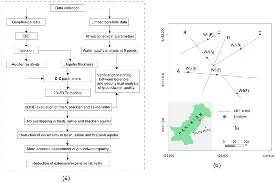
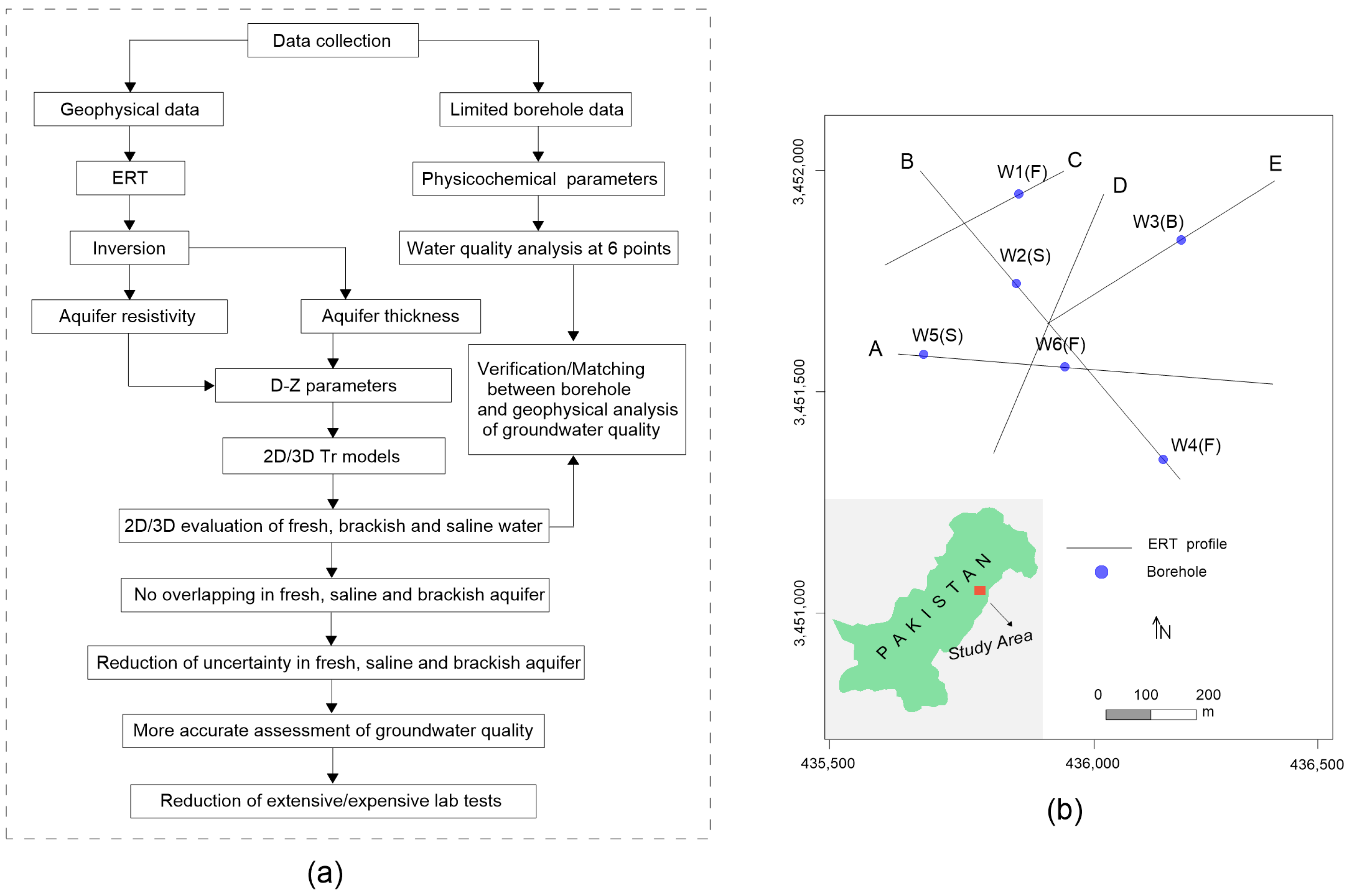
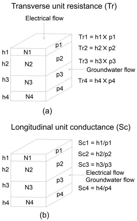
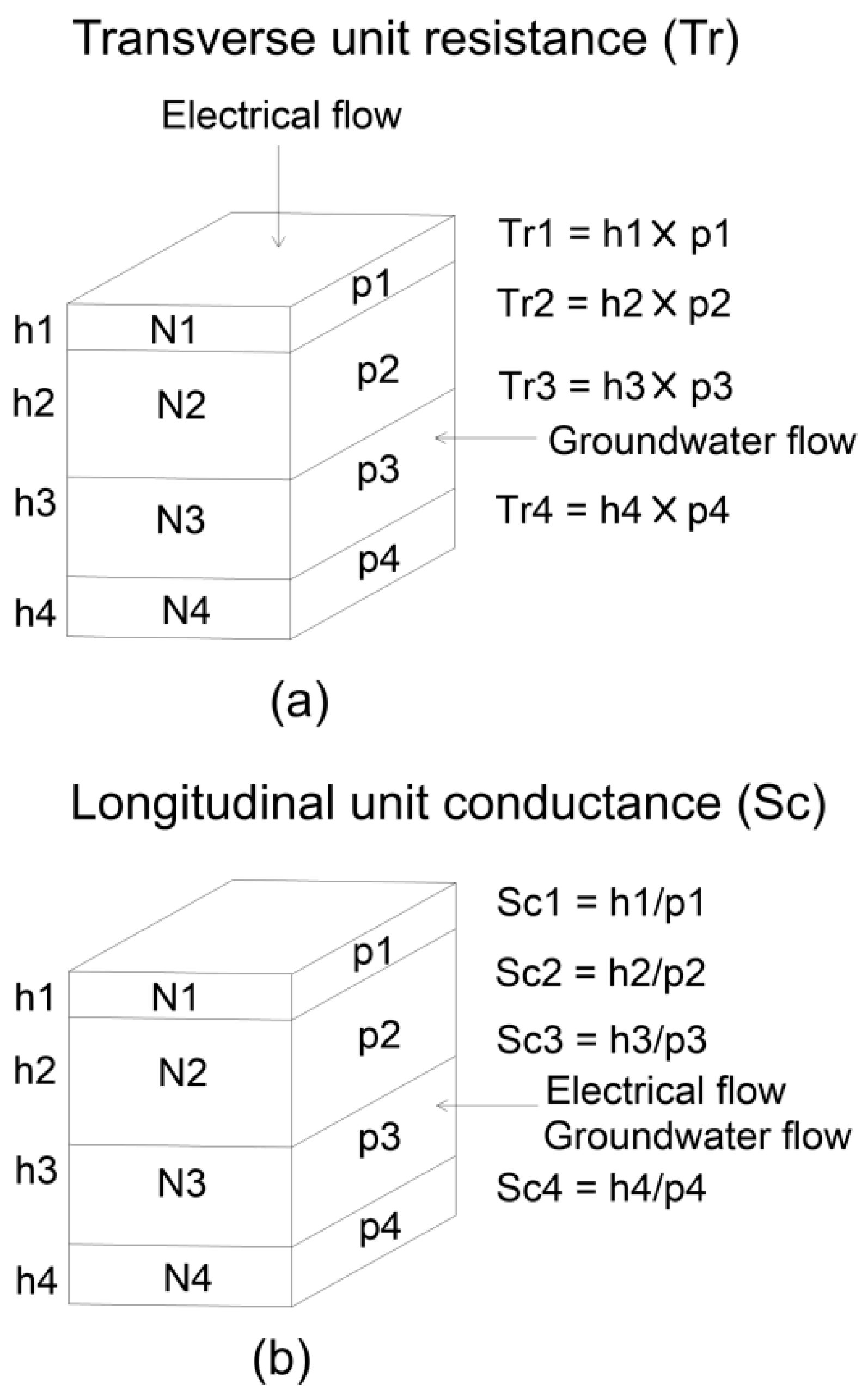
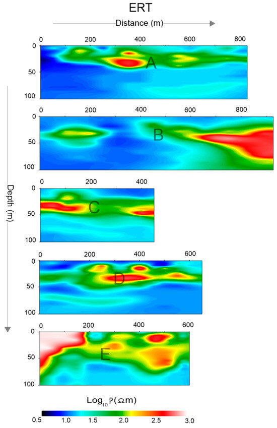
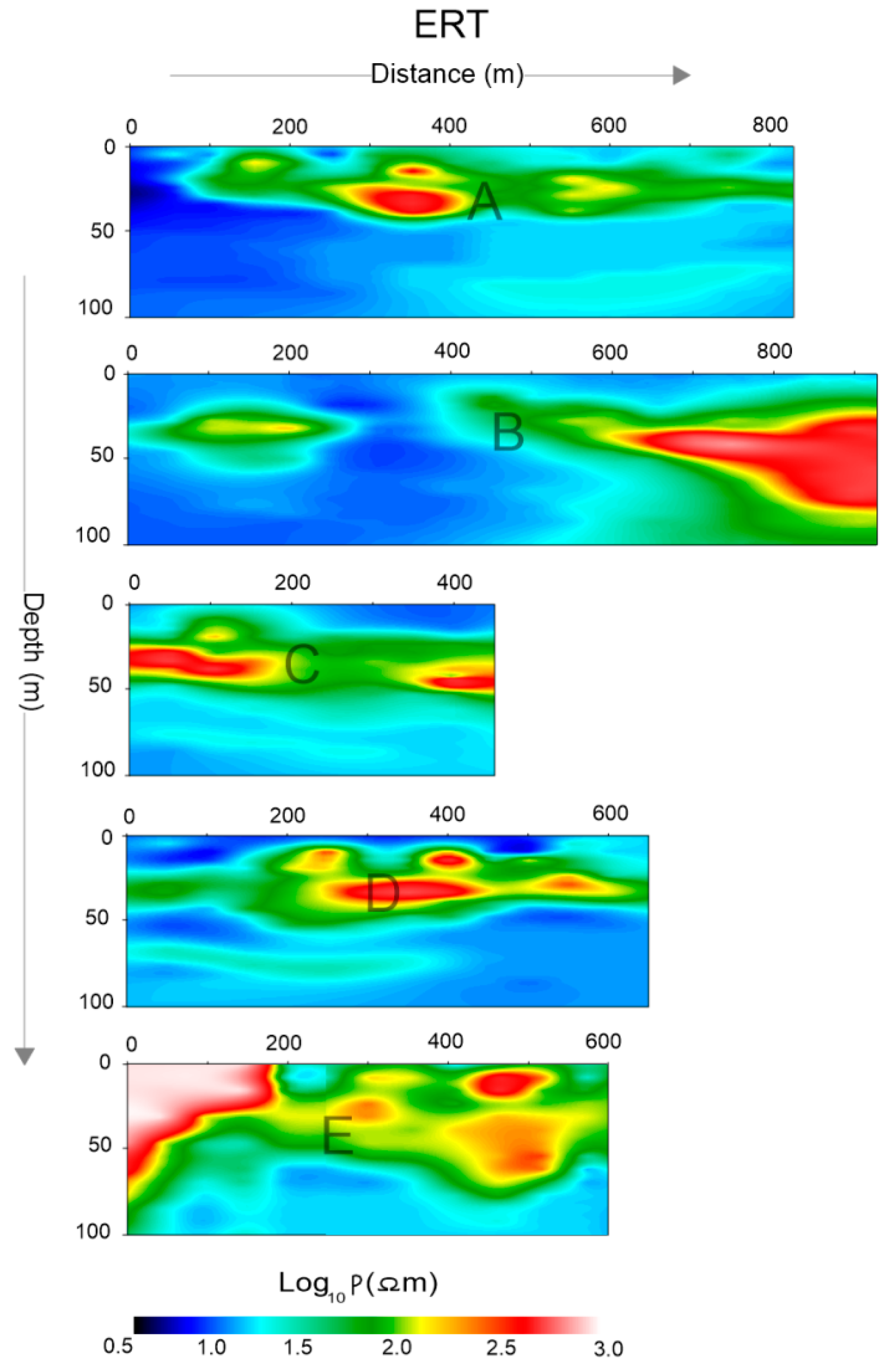
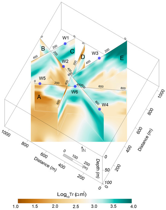
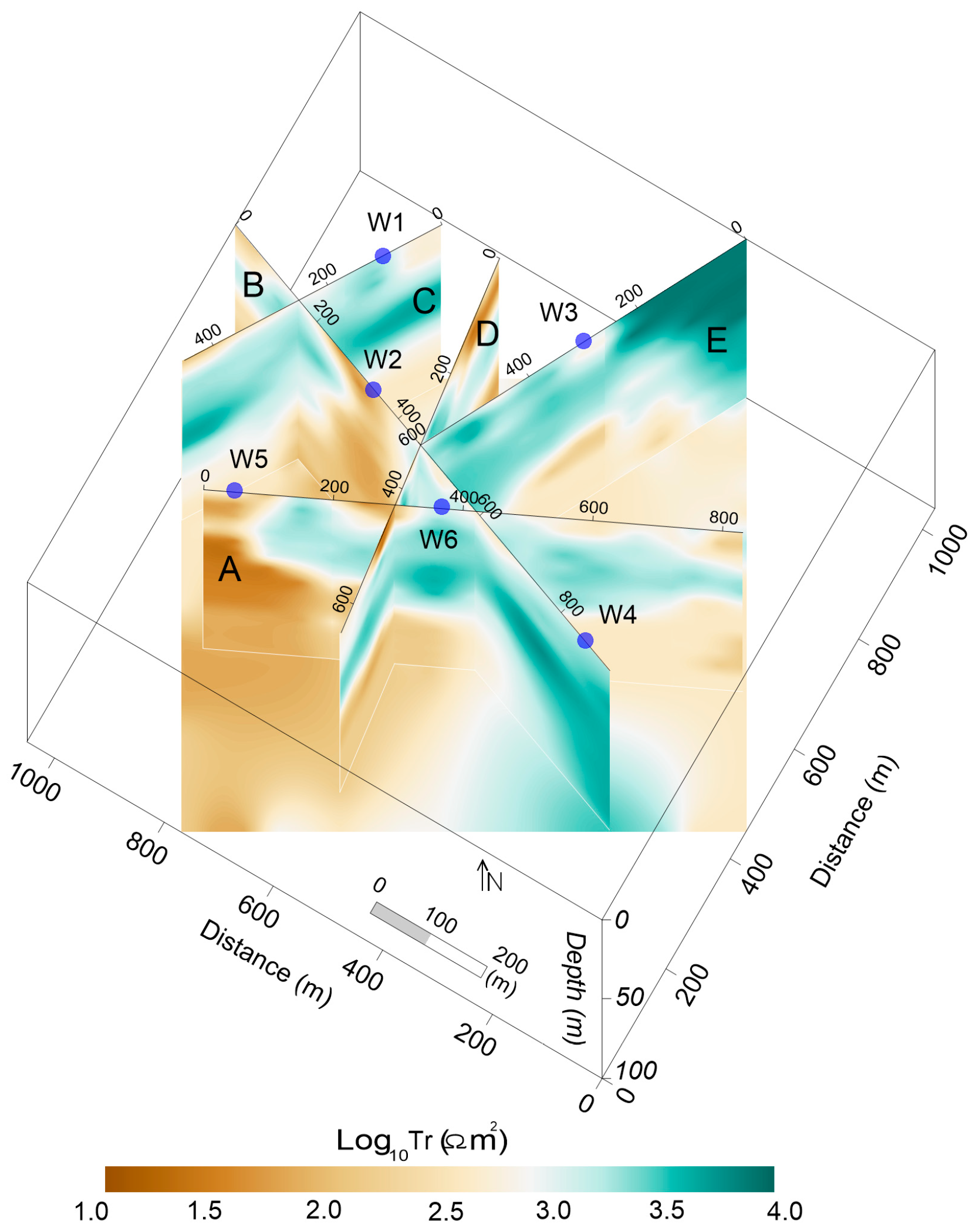
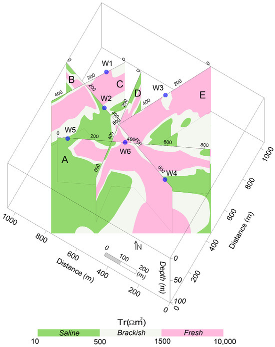
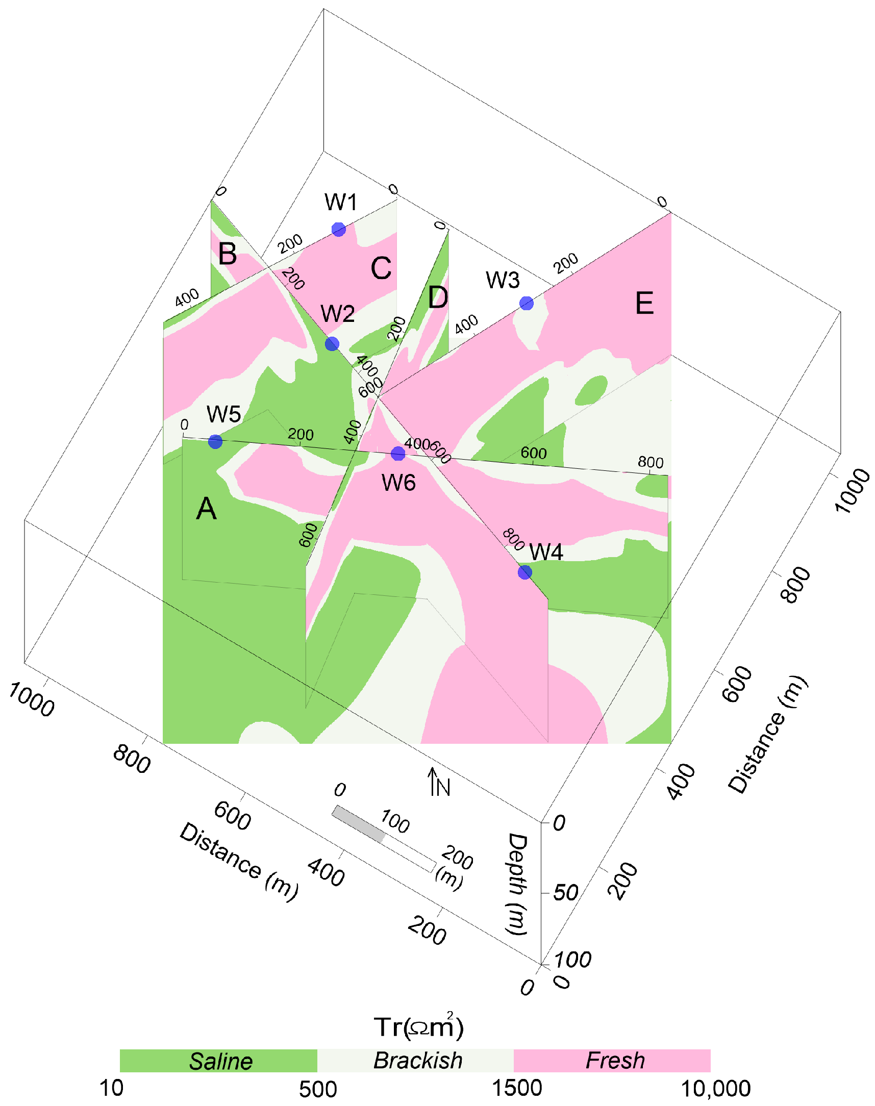
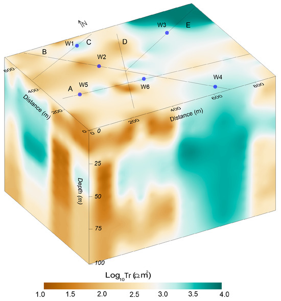
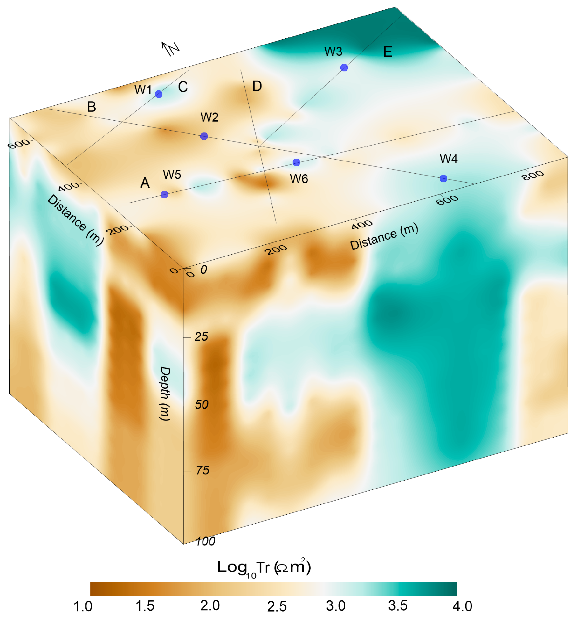
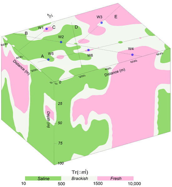
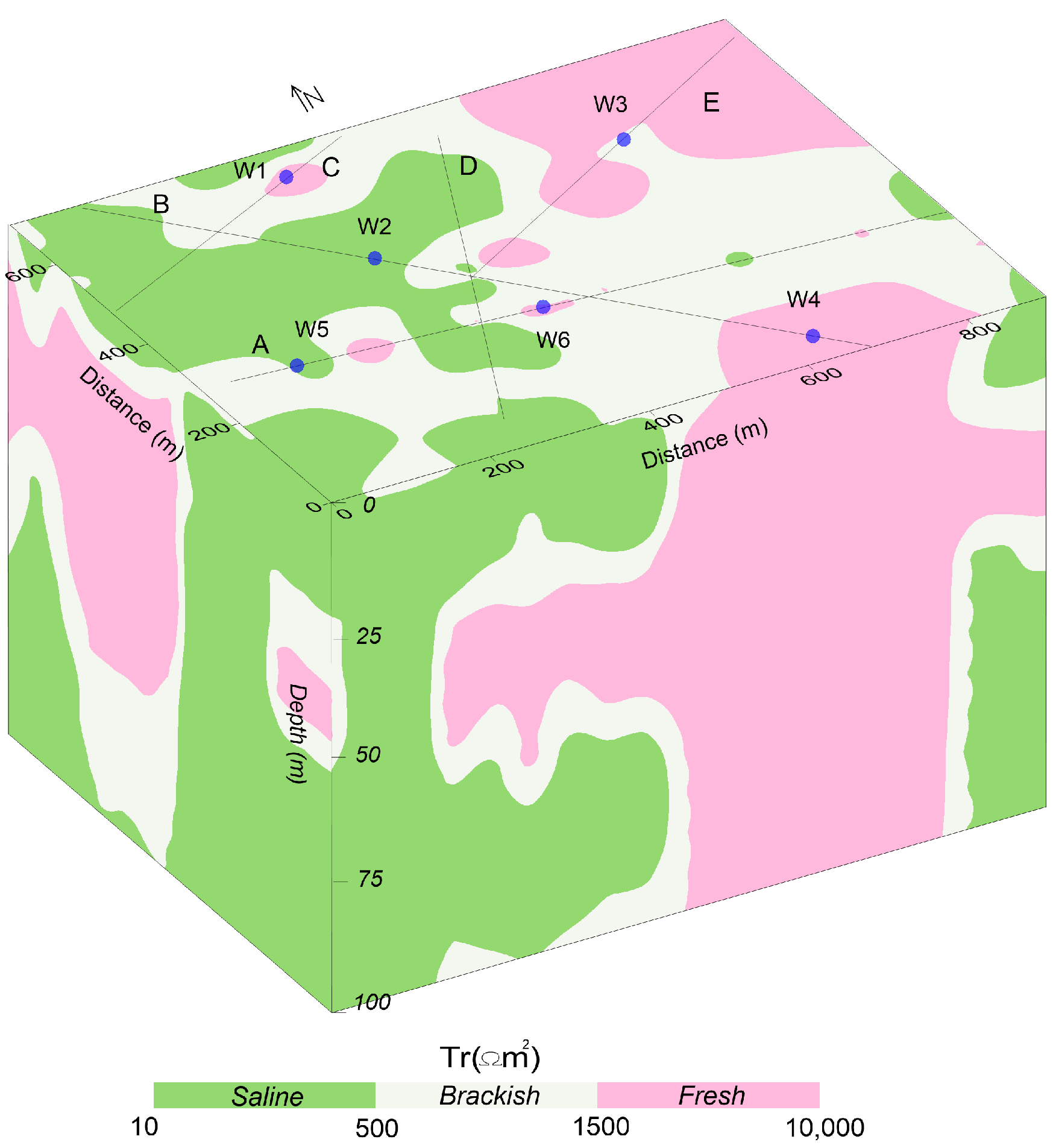
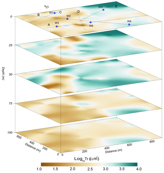
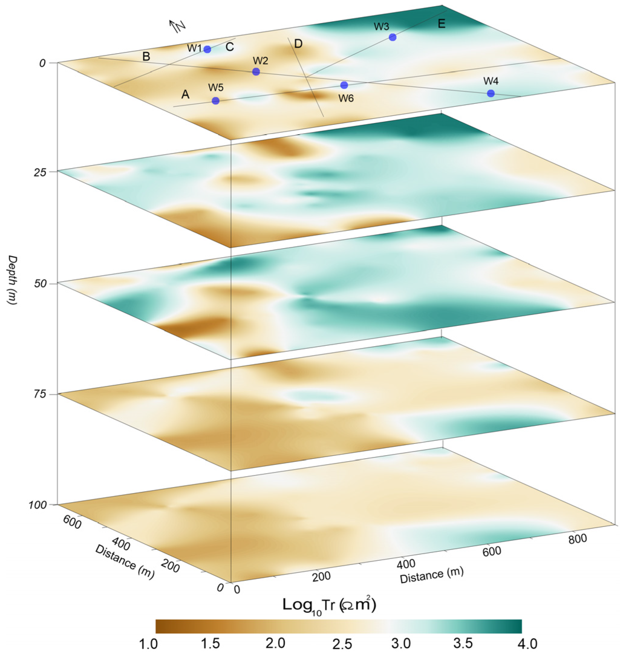
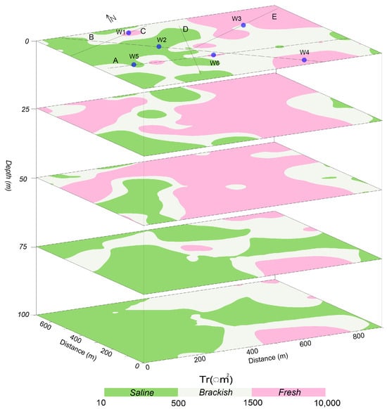
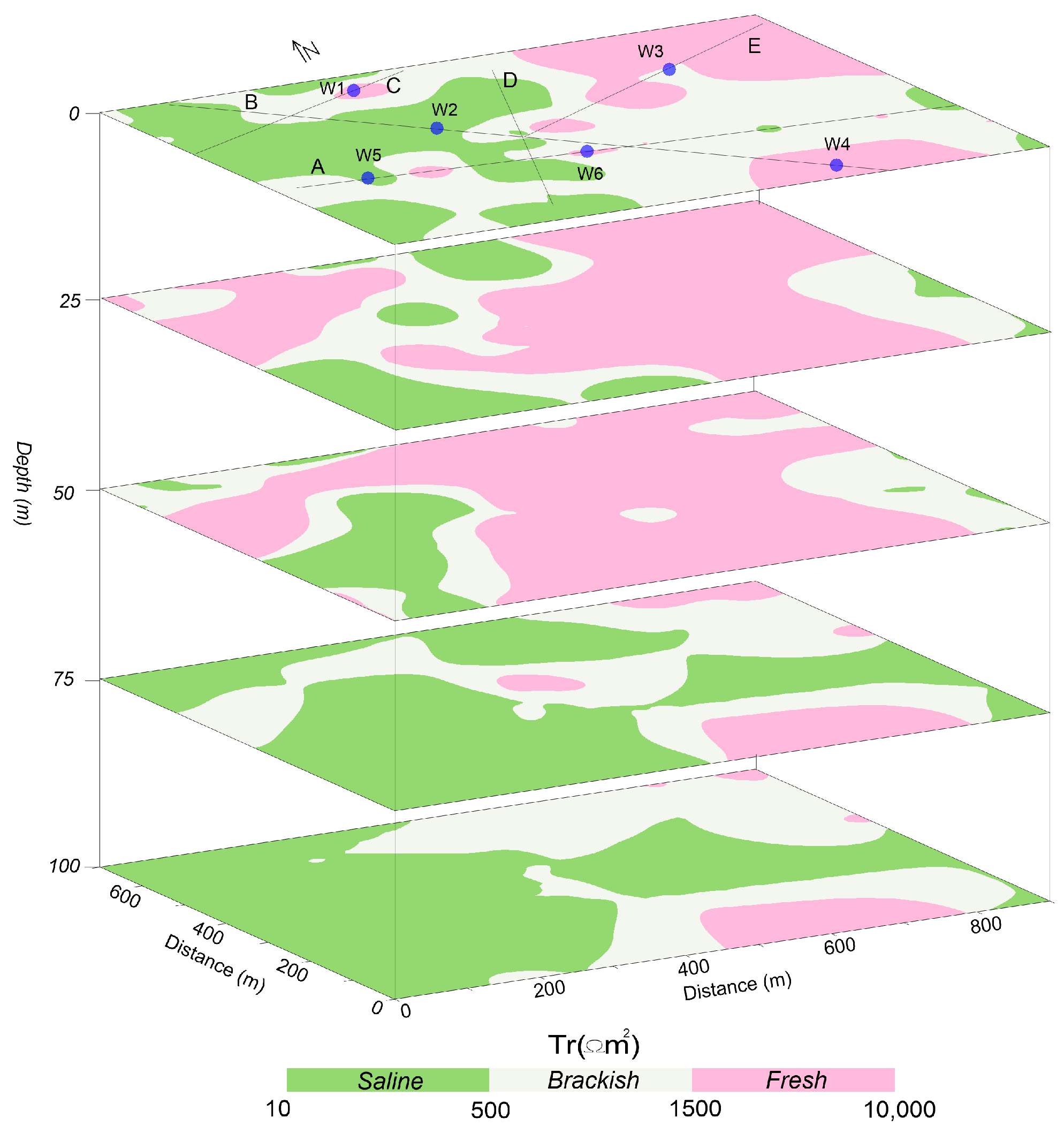

Disclaimer/Publisher’s Note: The statements, opinions and data contained in all publications are solely those of the individual author(s) and contributor(s) and not of MDPI and/or the editor(s). MDPI and/or the editor(s) disclaim responsibility for any injury to people or property resulting from any ideas, methods, instructions or products referred to in the content. |
© 2026 by the authors. Licensee MDPI, Basel, Switzerland. This article is an open access article distributed under the terms and conditions of the Creative Commons Attribution (CC BY) license.