Optimizing Performance of Equipment Fleets Under Dynamic Operating Conditions: Generalizable Shift Detection and Multimodal LLM-Assisted State Labeling

Abstract

This paper presents OpS-EWMA-LLM (Operational State Shifts Detection using Exponential Weighted Moving Average and Labeling using Large Language Model), a hybrid framework that combines fleet-normalized statistical shift detection with LLM-assisted diagnostics to identify and interpret operational state changes across heterogeneous fleets. First, we introduce a residual-based EWMA control chart methodology that uses deviations of each component’s sensor reading from its fleet-wide expected value to detect anomalies. This statistical approach yields near-zero false negatives and flags incipient faults earlier than conventional methods, without requiring component-specific tuning. Second, we implement a pipeline that integrates an LLM with retrieval-augmented generation (RAG) architecture. Through a three-phase prompting strategy, the LLM ingests time-series anomalies, domain knowledge, and contextual information to generate human-interpretable diagnostic insights. Finaly, unlike existing approaches that treat anomaly detection and diagnosis as separate steps, we assign to each detected event a criticality label based on both statistical score of the anomaly and semantic score from the LLM analysis. These labels are stored in the OpS-Vector to extend the knowledge base of cases for future retrieval. We demonstrate the framework on SCADA data from a fleet of wind turbines: OpS-EWMA successfully identifies critical temperature deviations in various components that standard alarms missed, and the LLM (augmented with relevant documents) provides rationalized explanations for each anomaly. The framework demonstrated robust performance and outperformed baseline methods in a realistic zero-tuning deployment across thousands of heterogeneous equipment units operating under diverse conditions, without component-specific calibration. By fusing lightweight statistical process control with generative AI, the proposed solution offers a scalable, interpretable tool for condition monitoring and asset management in Industry 4.0/5.0 settings. Beyond its technical contributions, the outcome of this research is aligned with the UN Sustainable Development Goals SDG 7, SDG 9, SDG 12, SDG 13.

1. Introduction

Industrial asset management has increasingly recognized the importance of accurate operational state awareness for complex equipment fleets. Power systems and other critical infrastructures deploy integrated supervisory control and data acquisition (SCADA) systems to monitor sensor data in real time and trigger alarms when abnormalities occur. However, current alarm systems configured with fixed thresholds or simplistic logic often perform inadequately in dynamic environments. They tend to produce a deluge of alarms (so-called “alarm floods”) during periods of system stress [1]. In such scenarios, operators face hundreds of alerts—many being false positives—which hinders their ability to discern truly critical events [2]. Even more concerning, important anomalies can be overlooked (false negatives) amid the noise. These issues can desensitize operators and have contributed to cascading failures in power networks when minor faults go unaddressed until they propagate into major outages [3]. In electrical grids sector, studies report that alarm floods obscure essential information and increase the risk of subsequent equipment failures downstream [4]. The underlying causes include suboptimal sensitivity settings, static prioritization rules, and inadequate filtering of redundant signals. This challenges the reliability and situational awareness of traditional alarm management frameworks.

To mitigate alarm overload, researchers have proposed advanced alarm management techniques [5]. Broadly, two families of methods exist: (1) sequence mining approaches, which ignore time-series dynamics but identify frequent patterns or sequences of alarm events leading to faults, and (2) time-series analytics, which focus on temporal behavior to spot anomalies. Various strategies have been explored—alarm correlation and similarity analysis, pattern extraction, classification and clustering of alarms, predictive alarm filtering, and dynamic suppression of nuisance alarms [6]. These have achieved some success in isolating critical alarms and reducing false alerts. For instance, techniques for alarm flood classification using multi-sensor data fusion have been developed to diagnose root causes during alarm cascades [3]. In the wind energy domain, clustering analysis of turbine alarm logs has been used to group related events and link them to downtime incidents [7]. A prescriptive framework combining SCADA sensor trends with alarm logs was shown to improve wind turbine fault prediction, underscoring the value of integrating heterogeneous alert data [8]. However, a major limitation of many alarm-management solutions is their lack of generalizability. They often require tailoring to each specific alarm system or equipment type, involving ad hoc rule tuning or training bespoke machine learning models for every component class. The development and maintenance effort for these custom solutions is substantial and applying them across different systems is non-trivial.

Given these challenges, there is a clear trend in industry and academia toward leveraging the wealth of raw sensor data directly for condition monitoring and anomaly detection [9]. Instead of relying on biased alarm outputs, modern approaches use data-driven algorithms on multivariate time-series (MVTS) from equipment sensors to identify abnormal behavior indicative of incipient faults [10]. This shift promises more objective and generalizable detection of equipment health issues. A rich body of work on anomaly detection in MVTS has emerged, ranging from classical statistical process control to advanced machine learning and deep learning techniques [11,12,13,14]. Traditional statistical methods include “memory-based” control charts like CUSUM (Cumulative Sum) and EWMA (Exponentially Weighted Moving Average), which are designed to raise alerts on shifts in a process signal’s mean or variance [15]. Modern enhancements to control charts include time-varying or adaptive smoothing factors to improve responsiveness and methods to automatically optimize the EWMA parameter for specific noise characteristics [16]. Such techniques have been applied in manufacturing and process engineering with success in early shift detection. Nonetheless, when scaling to dozens of sensor signals across large fleets, even tuned control charts face challenges—especially if each sensor requires separate parameter calibration or if signals are cross-correlated.

Parallel to statistical methods, data-driven machine learning (ML) approaches have flourished for anomaly detection and predictive maintenance. Unsupervised methods, supervised classification, and semi-supervised or hybrid strategies have all been reported [17]. These include distance or density-based outlier detectors, clustering algorithms to identify groups of abnormal points, subspace methods focusing on important feature projections, and ensemble techniques that combine multiple detectors. In the wind turbine context, deep learning models like autoencoders and recurrent neural networks (RNN) have been employed to learn normal behavior from historical SCADA data and flag deviations. Variational autoencoders and LSTM-based generative adversarial networks have shown promise in detecting subtle anomalies in turbine sensor streams [14]. Techniques such as temporal convolutional networks with robust distance metrics, and isolation forests or k-NN applied to high-frequency data, have achieved high true-positive rates in identifying anomalies [18]. A recent evaluation compared several ML and deep learning methods on multivariate industrial time-series and highlighted the trade-offs in detection accuracy and diagnosis capability. A key insight from these studies is that purely data-driven models can indeed uncover problems missed by alarm systems (reducing false negatives) and cut down false alarms [19]. However, they typically require substantial historical failure data for training and careful hyperparameter tuning per application. Each component or fault mode might need a custom-trained model, limiting scalability across diverse fleets. Additionally, complex ML models often act as “black boxes,” making it hard for engineers to interpret why an anomaly was flagged—a significant issue in sensitive industrial applications requiring trust and explainability.

Our approach addresses the above gaps by combining a simple yet powerful statistical detection method with the adaptability of modern AI for interpretation. Recent advancements in generative AI and foundation models have shown that LLMs are capable of reasoning over both structured and unstructured data to assist in tasks like troubleshooting and root cause analysis [20]. However, deploying these foundation models in industrial settings comes with challenges. General-purpose LLMs often lack specific domain knowledge and can produce hallucinations or irrelevant answers if prompted naively. To overcome this limitation, academic research has introduced a retrieval-augmented generation (RAG) approach [21]. This strategy has been shown in other studies to greatly improve the quality and trustworthiness of LLM responses for fault diagnosis [22]. Within a full fleet management pipeline, detection remains the domain of statistical or machine learning methods, while LLMs—augmented with RAG—add value through diagnosis and decision support.

In our prior work, we introduced a straightforward MVTS anomaly detection technique based on a residual EWMA statistic, which offers generalizability across equipment types. The method yields to an OpS-Matrix where each entry indicates if a given component on a given equipment is in a normal (0) or deviating (1) state at a given time interval [23]. We extend our approach by integrating an LLM-based component that can ingest the OpS-Matrix outputs along with other data modalities (technical documentation, maintenance logs, operator notes, etc.) to automatically label the anomalies using context-specific information. We implement the LLM reasoning in a multi-phase hierarchy: Phase I examines anomalies at the individual component level and generates a preliminary explanation. Phase II then considers the equipment level—aggregating all component anomalies on the same equipment—to infer the overall equipment state. Phase III generalizes across the fleet or operational context, translating multiple equipment-level findings into high-level overview of operational performance. This phased prompt design aligns with best practices in prompt engineering, allowing the LLM to tackle complex reasoning in steps and incorporate intermediate feedback [24].

Through the above integration of OpS-EWMA and LLM in one pipeline, our approach contributes a novel generalizable and interpretable anomaly management framework (

Table 1. Comparative overview of anomaly detection and diagnostic frameworks with OpS-EWMA-LLM positioning.

Method	Detection Core Mechanism	LLM Reasoning + Knowledge Integration	Outputs + Scale of Applicability	Distinctive Features/Limitations
Classical SPC-based methods (Shewhart, CUSUM, EWMA, PCA–T2)	Univariate/multivariate control charts	None (no LLM; no RAG/KG)	Binary control-limit breach per variable; limited to equipment-level monitoring	Interpretable, lightweight; no diagnostics
ML/DL anomaly detectors (autoencoders, LSTM–VAE, TCN, GAN, etc.)	Data-driven anomaly scoring/reconstruction-error–based detection	None (no LLM; no RAG/KG)	Anomaly score or binary label; limited generalizability across heterogeneous fleets	High accuracy but requires training; black-box
RAG-enhanced LLM diagnostic assistants (RAG-GPT, HybridRAG, LLM + KG frameworks)	External detector (rule-based, ML or alarms)	LLM explanations grounded via RAG or KG	Free-text diagnostic narratives; asset or plant-level rather than fleet-wide	Good explanations; weak detection integration
AAD-LLM/RAAD-LLM frameworks (SPC + feature extraction + LLM)	SPC statistics + DFT features	RAG injects historical thresholds or statistical references; LLM acts as classifier	Binary anomaly decision per sensor window; limited multi-asset generalization	Adaptive baseline updates; no semantic scoring
Proposed OpS-EWMA-LLM	Residual EWMA on fleet baselines producing OpS-Matrix	Hierarchical multi-phase LLM reasoning enriched with RAG technical documents	Structured operational state labels (Normal/Warning/Critical) with fleet-wide applicability	Hybrid pipeline: statistical rigor + semantic reasoning + dual scoring

) which is further distinguished by a structured interaction mechanism where residual-based fleet-normalized deviations (OpS-Matrix) explicitly guide hierarchical LLM reasoning, enabling diagnostic interpretability and scalability beyond existing SPC–LLM or RAG-enhanced detectors.

The contributions of this work can be summarized as follows:

• Generalizable Shift Detection: We develop a residual EWMA-based method that can be uniformly applied to monitor any subset of similar components in a fleet. It automatically compensates for common external influences by referencing fleet averages, enabling detection of true performance degradation with minimal false alarms. The approach is lightweight and easily scalable to hundreds of sensors, since it avoids intensive model training or complex tuning per sensor.
• Criticality Scoring Mechanism: We propose a three-phase, prompt-driven LLM pipeline that integrates time-series data with domain-specific textual knowledge. Through retrieval-augmented generation (RAG), the LLM is grounded in technical documentation and produces contextualized explanations of anomalies, including likely causes and potential remedial actions. Building on this, we introduce a severity index, which combines a statistical anomaly score with a semantic score derived from LLM reasoning. Unlike traditional labeling approaches, this dual-scoring process provides interpretable criticality levels for each event. The result is a structured repository of diagnostic cases enriched with graded severity labels, enabling more effective search, retrieval, and knowledge transfer across the fleet.
• Applicability to Wind Energy: We validate our approach on a real-world case study using SCADA data from 1997 wind turbines across 41 wind farms, demonstrating interpretable results that can directly inform asset management decisions.

The remainder of this paper is organized as follows. Section 2 reviews related work in condition monitoring, statistical shift detection, multimodal learning, and industrial AI to position our contributions in context. Section 3 details the OpS-EWMA methodology and the design of the LLM diagnostic pipeline. Section 4 presents the case study results. Section 5 concludes the paper and outlines future work toward scaling this framework and exploring its use in broader Industry 5.0 initiatives.

2. Literature Review

We begin with a survey of condition monitoring and predictive maintenance in wind power plants, then justify our statistical process control focus through a targeted review. We subsequently cover the latest diagnostic uses of generative AI—spanning time-series signals and textual/knowledge sources—and its practical implementations. This literature review motivates and informs the design of our framework.

2.1. Condition Monitoring and Predictive Maintenance

Condition monitoring aims to assess the health of equipment in real time, enabling predictive maintenance actions before catastrophic failures occur. Wind turbines, as complex electromechanical systems operating in variable conditions, have been a major focus of condition monitoring research [25]. Traditional turbine monitoring relies on SCADA measurements (e.g., temperatures, pressures, power output, vibrations) and threshold-based alarms for each signal, which led to alarm floods and missed faults. These limitations have prompted researchers to leverage the rich multivariate time-series data directly, using statistical and machine learning techniques to holistically detect incipient faults before catastrophic failures. The standard workflow models normal turbine behavior from historical data and flags deviations that either exceed statistical limits or resemble patterns of known failures [26]. Both physics-based models—such as thermodynamic models of gearboxes [27] or drivetrain dynamics [28]—and data-driven models have been employed, often in the context of “digital twins” that replicate the behavior of turbine subsystems under current conditions (

Table 2. Summary of fault detection model categories.

Model Categories	Description	Strengths	Limitation	Paper
Knowledge-Based Methods	Use expert knowledge to identify potential faults. Examples include rule-based systems, expert systems, and fuzzy logic.	Leverage domain expertise to make accurate predictions even with relatively little data.	Rely heavily on the availability and quality of expert knowledge, which may not be available or may be expensive to acquire. Also, these methods might not adapt well to new or changing conditions that weren’t anticipated by the experts.	[31,32]
Model-Based Methods	Rely on mathematical models that describe the physical behavior of the system. Examples include physics-based models, fault trees, and reliability models.	Very accurate when the model correctly describes the system, and they can also provide insight into the underlying physical processes.	The accuracy of these methods is heavily dependent on the accuracy of the model. Building accurate models can be challenging, especially for complex and nonlinear systems. These methods can also be computationally intensive.	[33,34]
Data-Driven Methods	Rely on historical data to identify patterns or anomalies that might indicate a fault. Examples include statistical methods, machine learning, and deep learning.	Handle complex, nonlinear systems, and they can potentially discover unexpected patterns or faults.	Require large amounts of high-quality, labeled data, which can be difficult to obtain, particularly for rare faults. Also, many data-driven methods (like deep learning) are “black box” models that can be difficult to interpret.	[35,36]

) [29]. By continuously comparing observed sensor data against simulated baselines, digital twins enable not only state monitoring but also forecasting of future degradation trajectories [30].

Among data-driven strategies, machine learning methods applied to turbine SCADA data have advanced considerably. Reviews highlight the progression from simple thresholding to sophisticated AI-based detection frameworks, stressing the importance of domain-specific feature selection [37]. Unsupervised learning is particularly attractive since labeled fault data are rare. Clustering algorithms can segment turbine operating states, while deviations from clusters reveal potential anomalies. For example, a minimum spanning tree-based anomaly detector has shown strong performance in hydropower turbine monitoring by efficiently approximating distances in high-dimensional data [38]. Deep learning approaches have demonstrated even higher promise: a temporal convolutional network (TCN) combined with a dynamic Mahalanobis distance threshold enabled the detection of subtle anomalies in turbine streams under varying wind conditions [39]. Likewise, a semi-supervised LSTM-based variational autoencoder with a WGAN (Generative Adversarial Network) learned normal operating behavior with minimal labeled data and successfully identified abnormal patterns [14]. These approaches generally outperform conventional SCADA alarms, offering earlier and more reliable detection. However, they also highlight the trade-off between sensitivity and specificity: overly sensitive detectors may misclassify benign variations (e.g., daily temperature cycles or wind gusts) as faults, whereas conservative thresholds may delay fault recognition.

An additional challenge lies in the heterogeneity of turbine fleets: models trained on one turbine type, manufacturer, or climate regime often fail to generalize across different sites. To address this, research increasingly explores transfer learning and domain adaptation, which recalibrate models with limited new data for different operating contexts. At the same time, explainability has emerged as a critical requirement. Given the high cost of false alarms and shutdowns, operators must trust diagnostic outputs; thus, explainable AI (XAI) techniques such as SHAP value analysis, saliency mapping, or rule extraction are now commonly integrated to interpret black-box model decisions [40]. Hybrid approaches also combine unsupervised clustering with rule-based expert systems, enabling distinction between sensor malfunctions and true equipment faults [41]. These strategies help balance performance with interpretability, an essential factor in operational adoption.

In parallel, classical statistical process control (SPC) methods have experienced renewed interest because of their computational efficiency and interpretability. SPC techniques fall into two families: multivariate control charts (MCCs) and univariate control charts (UCCs). MCCs, often combined with dimensionality reduction methods such as principal component analysis (PCA), can effectively track correlations among interdependent variables and provide a holistic representation of equipment health [32]. However, MCCs compress multivariate information into a single chart, limiting insight into variable-specific contributions. Complementary use of UCCs applied individually to each variable, followed by correlation analysis, can help disaggregate contributions to anomalies [32]. Complementary use of UCCs applied individually to each variable, followed by correlation analysis, can help disaggregate contributions to anomalies [33]. Widely used industrial UCC methods include Shewhart charts for rapid detection of large deviations, cumulative sum (CUSUM) charts and exponentially weighted moving average (EWMA) charts for detecting smaller shifts, and attribute-based charts (e.g., p-charts or u-charts) for binary outcomes [34,35]. Recent advances introduce adaptive smoothing factors and optimized parameter tuning to improve responsiveness under noisy conditions, making SPC tools viable for high-dimensional and dynamic wind turbine data. While limitations remain, these methods provide lightweight and interpretable complements to data-intensive AI models, especially in contexts demanding real-time operational monitoring [37]. These issues are addressed and solved in the methodology section.

In summary, condition monitoring in wind energy has evolved from basic alarm thresholds to an array of advanced techniques, including digital twins, statistical analysis, and machine learning. The literature encourages adaptations like residual charts and group comparisons to handle the complexities of real-world data. Our literature review finds that while advanced ML often grabs headlines, these statistical methods remain extremely valuable in industrial contexts due to their simplicity, transparency, and low requirement for fault examples. By leveraging an EWMA on residuals, our approach aligns with best practices from these studies, achieving robust anomaly detection without a need for extensive training data. The next subsections will delve into how we augment such statistical detection with AI-driven interpretation.

2.2. Anomaly Detection and Diagnostics with Generative AI

The advent of large-scale language models (LLMs) has significantly expanded the methodological landscape for fault detection and diagnostics (FDD) in engineering and energy systems. Large Language Models (LLMs) like OpenAI’s GPT series, Google’s BERT-derived models, and domain-adapted transformers have shown the capacity to capture semantics across technical domains when properly tuned or guided. Their application in industrial maintenance is an active area of research [42]. Early studies demonstrated their utility in analyzing unstructured maintenance-related text, such as work orders, error logs, and technician notes, to extract latent knowledge about equipment health and operational reliability. These applications highlight an evolution beyond conventional natural language processing (NLP) methods, where rule-based or shallow statistical models were often insufficient to capture the nuances of technical vocabulary and fault progression dynamics [43]. By leveraging contextual embeddings and generative capabilities, LLMs can identify implicit relations between operational events and failure modes, forming a foundation for AI-enhanced predictive maintenance in complex infrastructures. Beyond text-based mining, an important development has been the emergence of multimodal LLM frameworks—in which the model serves as a central reasoning engine capable of fusing heterogeneous inputs such as sensor time series, images, and operator narratives. A recent framework leveraging a 32-billion-parameter LLM for predictive maintenance of industrial compressors demonstrated that multimodal fusion improves anomaly recall and interpretability relative to specialized CNNs and LSTMs [44]. The self-attention mechanism of transformers enables capturing dependencies across modalities, linking sensor-derived features with textual fault descriptions and visual cues. Notably, the Qwen 2.5–32B model achieved superior performance in anomaly detection while also generating natural language explanations that could be directly interpreted by operators, thereby reducing false alarms and lowering operational costs. These findings underscore the potential of multimodal LLMs to bridge low-level data-driven diagnostics with high-level decision support in asset management.

To operationalize LLMs for industrial FDD, researchers have relied on prompt engineering and domain adaptation strategies. A common practice is to use a system prompt to establish the diagnostic context, followed by a structured user prompt encoding heterogeneous state information, including numerical sensor readings, alarm messages, inspection images, and expert annotations—often in JSON or tabular form [45]. Within Industry 4.0 scenarios, GPT-4 has been applied in this manner, successfully identifying anomalies across diverse equipment types by formatting sensor metadata as natural language text [46]. However, such approaches face challenges of reliability: LLMs may produce plausible but incorrect diagnoses when prompts are underspecified or when training data lacks domain specificity. To mitigate these risks, techniques such as knowledge infusion through domain-specific fine-tuning have been explored [47]. Yet, fine-tuning very large models remains resource-intensive and inflexible in dynamic environments where knowledge updates are frequent. Retrieval-augmented generation (RAG) has emerged as a more scalable and practical alternative, enabling LLMs to dynamically access external knowledge sources rather than embedding all domain knowledge within their parameters. In RAG-based systems, external databases, fault logs, or knowledge graphs are queried in real time and appended to the prompt, enhancing both factual accuracy and domain alignment [48]. Recent work has shown that RAG-enhanced ChatGPT, using gpt-3.5-turbo-0301 and gpt-4, can substantially improve diagnostic accuracy when provided with structured repositories of equipment manuals and maintenance logs [49]. Further, hybrid approaches such as “HybridRAG”, integrate retrieval with knowledge graphs, combining the interpretability of symbolic reasoning with the generative flexibility of LLMs [50]. These frameworks represent a transition point in the literature: moving from static expert systems and narrow deep learning models toward adaptive, explainable, and knowledge-grounded AI assistants that can operate reliably in industrial FDD contexts.

A particularly recent relevant development is RAAD-LLM (Retrieval-Augmented Adaptive Anomaly Detection with LLMs) framework, an enhanced version of AAD-LLM (Adaptive Anomaly Detection using LLMs) method which leveraged a pretrained language model in a zero-shot manner to detect anomalies in time-series sensor data. RAAD-LLM augments the original framework with a RAG component to inject relevant reference knowledge into the LLM’s prompt. Each new time-series window from the equipment is first analyzed using statistical process control (SPC) techniques and signal processing. RAAD-LLM computes control chart metrics and a Discrete Fourier Transform (DFT) on the data to extract key features. z-scores are then injected into a templated text prompt. The RAG module uses those statistics as a query to retrieve context from a domain knowledge base (historical operating ranges and previously observed z-score thresholds). The retrieved contextual information is appended to the prompt alongside the live data descriptors. The LLM (8-billion-parameter LLaMA 3.1 model) remains frozen and is asked, in this richly informed prompt, to output whether the current conditions represent a high deviation (anomaly) or not. The answer is then parsed (via a simple rule-based function) into a binary decision, and the system updates its baseline with the new data if it was deemed normal. This last step implements an adaptability mechanism: RAAD-LLM continually refreshes its understanding of “normal” as operations evolve, addressing concept drift in a non-parametric way [51].

Beyond these targeted applications, researchers are investigating how to generally repurpose LLMs for time-series analysis tasks. Time series analytics traditionally includes forecasting, classification, anomaly detection, and imputation [52]. Until recently, forecasting dominated the intersection of LLMs and time-series: Time-LLM showed that by “reprogramming” numerical sequences into natural-language-like prompts, a frozen GPT-style model could perform competitive time-series forecasts without any gradient training [53]. Similarly, Chronos method tokenized time-series data into a vocabulary of symbols to feed a language model, avoiding dataset-specific retraining and achieving strong zero-shot predictions [54]. These approaches indicated that LLMs’ pattern recognition abilities can transfer to sequential sensor data when the input is appropriately encoded. To remove the need for manual prompt design, other frameworks trained dedicated embedding layers: a unified model (One-Size-Fits-All, OFA) that learns a numeric embedding to interface with a frozen LLM, enabling tasks like univariate anomaly detection and few-shot classification [55]. Another study proposed an embedding alignment method (TEST) to map time-series signals into the text embedding space of an LLM [56]. Like OFA, TEST required training a front-end, but it allowed the LLM to handle multiple time-series tasks without sacrificing its language capabilities. These works demonstrate various embedding strategies for combining sequence data with generative models. Notably, however, most early efforts were limited to single-sensor or simulated data and focused on performance metrics; they did not tackle rich multivariate anomaly detection or interactive diagnostics in real industrial contexts. Overall, these pioneering steps in univariate time-series analysis using LLMs demonstrate that foundation models are capable of capturing temporal structure (trend, seasonality, periodicity, etc.). Building on this insight, we embed temporal characteristics of time-series directly into the prompt structure, enabling the model to reason over both short-term fluctuations and long-term patterns.

This review of prior work on alarm management, multivariate time-series anomaly detection, statistical process control, and LLM-based diagnostics, establishes the foundation for a unified framework that is generalizable, scalable, and interpretable, thereby enhancing anomaly detection and diagnostics across heterogeneous equipment fleets. Within our broader research on the resilience of electrical systems, such a framework addresses previous challenges in assessing the distribution of operational states under varying conditions. Moreover, deploying this model in industrial settings redefines the operator’s role: rather than engaging in low-level data sifting, human expertise is directed toward verification and strategic decision-making informed by AI-generated insights. This shift aligns with the vision of Industry 5.0, which emphasizes human-centric technology—operators are supported by AI in routine tasks and can focus on higher-level judgments [57]. The next section will detail how OpS-EWMA is designed and how the LLM component is integrated in the pipeline, drawing on these insights to fulfill the objectives of generalizable shift detection and explainable operational state labeling across an equipment fleet.

3. Methodology

In the industrial context, the process of labeling the operational states of equipment involves determining whether their functioning is normal, abnormal, or transitioning to a critical state at each moment t or at regular time intervals $\delta t$. This process uses the data recorded by sensors installed on the equipment components. The collected data includes physical measurements such as temperature, pressure, frequency, vibrations, etc., at high frequency, thereby creating time series (TS) [58]. Multivariate TS analysis techniques such as classification (by segment) and anomaly or fault detection are employed at this stage to identify deviations from normal operation, indicating observations or sequences of observations in a critical state. These techniques fall under the broader category known as condition monitoring. They include “memory-based” charts such as CUSUM and EWMA [15]. While both aim to identify deviations in time series data, they operate on different principles in terms of sensitivity to shifts and data weighting. Given the fluctuations and high variability in physical data measurements, EWMA is particularly interesting [59]. It applies weighting factors that decrease exponentially, giving more weight to recent observations without completely disregarding older ones. This method smooths short-term fluctuations and highlights long-term trends or cycles in equipment. The EWMA statistic for the process $X$ is calculated using the following formula:

$$Z_t=\left\{\begin{array}{ll}{Z}_0,& t=0\\ {\lambda ·X}_t+\left(1-\lambda \right)·Z_{t-1},& t>0\end{array}\right.$$

(1)

where $Z_t$ is the EWMA statistic at time $t$, $X_t$ is the process at time $t$, and $\lambda$ is the smoothing parameter between 0 and 1. If $\lambda$ is close to 1, the smoothing is very weak, giving great importance to recent values. In the case where $\lambda =1$, the EWMA statistic becomes a Shewhart map. On the other hand, if $\lambda$ is close to 0, the control map has a large memory and gives greater weight to historical values. The smoothing constant must therefore be chosen according to the type of variation to be detected. To choose the value of parameter $\lambda$, we need to have an idea of the amplitude of the variations likely to occur. Several approaches can be used to obtain the optimum value of $\lambda$ such as model-based calibration [60] or time-varying value adapted to the expected shift over the time [16]. The common performance measure for EWMA statistic is the expected time between false positive detections denoted average run length [61]. The optimal range of values for $\lambda$ is provided in [62,63].

The starting value $Z_0$ is the process target or expected value of $\overline{X}$. In real application, the central line of EWMA $Z_0$ is generally replaced by ${\mu }_0$, the average of preliminary data or selected period of historical data where the equipment is in normal operation status. Since the EWMA can be viewed as a weighted average of all past and current observations, it is very insensitive to the normality assumption. It is therefore an ideal control statistic to use with MVTS. The lower control limit (LCL) and the upper control limit (UCL) are defined by:

$$\begin{gathered} CL={\mu }_0\pm k {\sigma }_0={\mu }_0\pm k {\sigma }_{\overline{X}}\sqrt{{\displaystyle \frac{\lambda }{\left(2-\lambda \right)}} \left[1-{\left(1-\lambda \right)}^{2i}\right]} \\ \underset{i\to +\infty }{\to }{\mu }_0\pm k {\sigma }_{\overline{X}}\sqrt{{\displaystyle \frac{\lambda }{\left(2-\lambda \right)}}} \end{gathered}$$

(2)

where ${\sigma }_0$ is the standard deviation of the EWMA statistic, ${\sigma }_{\overline{X}}$ the standard deviation of the process $\overline{X}$ with independent random variables, and $k$ is the width of the control limits, usually set to $k=3$ correspond to a three-sigma limit or 99.9% confidence level.

As we are dealing with MVTS at very high resolution, a lot of noise perturbed the deviation detection process. One of the solutions that has been studied in the literature is applying the moving average to a residual $R$ also denoted $\mathsf{\Delta }$, expressed by the difference between physical quantity measure on an equipment and the expected value [64]. Generally, the expected value is computed using a model-based approach [65], or a machine learning or deep learning model trained on historical data such as bagged regression trees (RT) [66] or gaussian process regression (GPR) [58]. The problem with this method is that every type of component needs to be modeled, and it became excessively cost in computation and in model testing, hyperparameters turning, and data preprocessing. This approach performs well on a single component but is not appropriate to generalize to multiple types of physical measurement.

On of the solution found, is to take the variation between a specific component and the average of the remaining system fleet components [67]. This approach works with a minimum number of components to ensure the robustness of the fleet average. Let $\epsilon ·{\mu }_0$ denote the maximum acceptable impact on the average, ${\delta }_j·X_j$ the shift of the equipment $j$, $K$ the maximum number of equipment presenting a shift and $N$ the total number of equipment, then:

$${\mu }_0+{\displaystyle \frac{1}{K}}\sum _{j=1}^K{\delta }_j·{\displaystyle \frac{X_j}{N}}<{\mu }_0+\epsilon ·{\mu }_0$$

(3)

Which can be simplified to:

$${\displaystyle \frac{1}{K}}\sum _{j=1}^K{\delta }_j·{\displaystyle \frac{X_j}{N}}<\epsilon ·{\mu }_0$$

(4)

As equipment is in the same operating conditions during the interval time $\delta t$, ${\overline{X}}_{j, \delta t}\approx {\mu }_0$. Thus, the precedent inequality becomes:

$$N>{\displaystyle \frac{1}{\epsilon }}·{\displaystyle \frac{1}{K}}\sum _{j=1}^K{\delta }_j$$

(5)

Furthermore, as the physical quantities of components are affected by the operational condition, EWMA statistic should be computed on equipment located in a defined geographical area. This uniformity in operating conditions across the same type of equipment implies that the variations in physical parameters like vibrations, temperatures or pressure remain consistent across equipment and over time. The difference between the values measured by an equipment sensor and the fleet average should be statistically constant within the CL, if they operate in normal status.

For a given physical quantity measured on the equipment $i, i=0, \dots , N$, the difference with the mean of other equipment, denoted ${\mathsf{\Delta }}_{x_i}\left(t\right)$, can be defined by the following equation:

$$R_i\left(t\right)={\mathsf{\Delta }}_{x_i}\left(t\right)=x_i\left(t\right)-\sum _{k,k\ne i}^{N\left(t\right)}{\displaystyle \frac{x_k\left(t\right)}{N\left(t\right)-1}}$$

(6)

Variations in ${\mathsf{\Delta }}_{x_i}\left(t\right)$ indicate a change in the behavior of the component $i$. Detecting abnormal variations using ${\mathsf{\Delta }}_{x_i}\left(t\right)$ is more straightforward than using $x_i\left(t\right)$ as this method effectively isolates deviations specific to the equipment by eliminating stochastic fluctuations due to environmental effects and therefore decrease the noise in the observation. Consequently, in the EWMA statistic, the standard physical quantity observation $X_t$ is replaced by ${\mathsf{\Delta }}_x\left(t\right)$ in the Equation (1):

$$Z_i\left(t\right)=\lambda ·{\mathsf{\Delta }}_{x_i}\left(t\right)+\left(1-\lambda \right)·Z_i\left(t-1\right)$$

(7)

where ${\mathsf{\Delta }}_{x_i}\left(t\right)$ can be defined as a random variable from a normal distribution with mean ${\mu }_{\mathsf{\Delta }\overline{X}}$, and standard deviation ${\sigma }_{\mathsf{\Delta }\overline{X}}$ expressed with following formulas:

$${\mu }_{\mathsf{\Delta }\overline{X}}={\displaystyle \frac{1}{T}}\sum _{t=0}^T{\displaystyle \frac{1}{N}}\sum _{i=1}^N{\mathsf{\Delta }}_{x_i}\left(t\right)={\displaystyle \frac{1}{T}}\sum _{t=0}^T \overline{{\mathsf{\Delta }}_{x_i}\left(t\right)}$$

(8)

$${\sigma }_{\mathsf{\Delta }\overline{X}}={\displaystyle \frac{1}{T}}\sum _{t=0}^T\sqrt{{\displaystyle \frac{1}{N}}\sum _{i=1}^N\left({\mathsf{\Delta }}_{x_i}\left(t\right)-\overline{{\mathsf{\Delta }}_{x_i}\left(t\right)}\right)}$$

(9)

$$CL\cong {\mu }_{\mathsf{\Delta }\overline{X}}\pm k {\sigma }_{\mathsf{\Delta }\overline{X}}\sqrt{{\displaystyle \frac{\lambda }{\left(2-\lambda \right)}}}$$

(10)

At this stage, an alarm generation process needs to be defined. The simple rule is to raise an alarm when $n$ consecutive points are outside the CL. As we are working with high frequency data on physical quantities over the equipment’s operating time, the statistic is critical if it exceeds the upper control limit (UCL). To optimize the process, we perform an average resampling to the EWMA statistics and UCL with a selected frequency $\delta t$ (e.g., daily, weekly, etc.) and raise an alarm when a single point falls above the UCL. We define $Z_{i,\delta t}$ the vector of $K={\displaystyle \frac{T}{\delta t}}$ resample observations:

$$\overrightarrow{Z_{i,\delta t}}=\left(\begin{array}{c}{\displaystyle \frac{1}{\delta t}}{\displaystyle \sum _{t=0}^{\delta t}} Z_i\left(t\right)\\ ⋮\\ {\displaystyle \frac{1}{\delta t}}{\displaystyle \sum _{t=\left(K-1\right)·\delta t }^{K·\delta t}}{Z}_i\left(t\right)\end{array}\right)=\left(\begin{array}{c}\overline{Z_i}\left(0\right)\\ ⋮\\ \overline{Z_i}\left(K\right)\end{array}\right)$$

(11)

$$\overrightarrow{{UCL}_{\delta t}}=\left(\begin{array}{c}{\displaystyle \frac{1}{\delta t}}{\displaystyle \sum _{t=0}^{\delta t}} {UCL}_t\\ ⋮\\ {\displaystyle \frac{1}{\delta t}}{\displaystyle \sum _{t=\left(K-1\right)·\delta t }^{K·\delta t}}{UCL}_t\end{array}\right)=\left(\begin{array}{c}\overline{UCL}\left(0\right)\\ ⋮\\ \overline{UCL}\left(K\right)\end{array}\right)$$

(12)

As control limit converge to UCL value, $\overrightarrow{{UCL}_{\delta t}}$ is a constant vector and the accuracy of the threshold depends on the number $N$ of equipment used to compute the statistic.

At this stage, we use only one physical measurement at a time to determine the operational status of a component type on a set of equipment. To assign a criticality factor at each interval $\delta t$ for a given piece of equipment, we need to consider the interdependencies between these components. To do so, we define a binary operational state matrix called the OpS-Matrix which indicates for each equipment the set of components whose operational state deviates from the normal state. If we have $N+1$ equipment on a selected location composed with $L+1$ common sensors, the OpS-Matrix is the following:

$$\begin{gathered} M_{OpS}\left(t\right)=\left(\begin{array}{ccc}{OpS}_{\mathrm{0,0}}\left(t\right)& \dots & {OpS}_{0,N}\left(t\right)\\ ⋮& \ddots & ⋮\\ {OpS}_{L,0}\left(t\right)& \dots & {OpS}_{L,N}\left(t\right)\end{array}\right), \\ \mathrm{Where} {OpS}_{i,j}\left(t\right)=\left\{\begin{array}{c}0, {\overline{Z}}_{i,j}\left(t\right)-{\overline{UCL}}_{i,j}(t)<0\\ 1, {\overline{Z}}_{i,j}\left(t\right)-{\overline{UCL}}_{i,j}(t)\ge 0\end{array}\right. \end{gathered}$$

(13)

If the value is 0, the component is in a normal state; if the value is 1, the component transitions to a critical state.

Given anomaly information for each component at a $\delta t$ sampling frequency, it becomes necessary to assess the criticality of equipment-level abnormal operating states. We address this through an LLM-driven diagnostic analysis implemented within a hierarchical three-phase prompting architecture. Each prompt is composed of three elements: a system prompt, a user prompt, and contextual data (

Table 3. Overview of the hierarchical three-phase LLM diagnostic framework with RAG integration. A consistent prompting structure that progressively aggregates knowledge and reasoning from individual sensors to fleet-wide insights.

Prompt Elements	Phase I	Phase II	Phase III
System	Assigns the role of component-level diagnostic assistant.	Defines the role as equipment-level synthesizer.	Defines the role as fleet-level analyst.
User	Contains the anomaly event packet for a single component.	Aggregates all component-level diagnoses for one piece of equipment.	Collects all equipment-level summaries across the fleet.
Contextual Data	Retrieves relevant manuals, fault databases, and maintenance logs related to that component/anomaly.	Retrieves subsystem interaction models, equipment manuals, and FMEA reports.	Retrieves fleet bulletins, cross-site maintenance reports, and industry alerts.
Assistance	Initial diagnosis for the component; may suggest immediate checks or corrective actions.	Integrated diagnosis of the equipment state; identifies subsystem interactions and higher-level fault patterns.	Comparative reasoning across units; detects systemic issues, recurring anomalies, or fleet-wide trends.

). To enhance the accuracy and reliability of the model’s outputs, we integrate a retrieval-augmented generation (RAG) process, enabling the LLM to ingest both anomaly descriptions and domain-specific documentation (retrieved context) in order to generate human-interpretable explanations or labels.

• Phase I—Component-Level Diagnosis: The system prompt establishes the role, and the user prompt supplies the event packet details (semantic summary a component’s anomaly). The prompt is enriched with RAG-retrieved domain knowledge (technical manuals, fault databases, maintenance records). The LLM then produces an initial diagnosis at the component level and possibly suggests immediate checks or actions.
• Phase II—Equipment-Level Synthesis: The user prompt in Phase II aggregates the outputs from Phase I along with any additional subsystem-level knowledge (e.g., equipment operation manuals or failure mode and effects analyses (FMEA)). The LLM performs reasoning across components to capture system-wide fault patterns, consistent with hierarchical fault modeling approaches reported in the literature [68].
• Phase III (optional)—Fleet-Level Reasoning: Finally, the model generalizes across multiple units to detect fleet-wide trends, identify recurring anomalies, and distinguish isolated issues from systemic problems. This step leverages collective insights and aligns with research advocating fleet-level anomaly detection frameworks [69].

After the LLM has provided diagnostic hypotheses at component, equipment, and fleet levels, the final stage of framework introduces a decision layer that consolidates these insights with the original statistical anomaly metrics. The objective of this layer is to assign each detected event a criticality state label $C_s, s=1,\dots ,S$ (e.g., Normal, Warning, Critical operational state) based on both quantitative anomaly severity and qualitative semantic assessment. The resulting set of labels forms the OpS-Vector that corresponds to the row-level labels of the OpS-Matrix:

$$\overrightarrow{{\mathrm{V}}_{\mathrm{O}\mathrm{p}\mathrm{S}}}=\left(C_{s_0} \dots , C_{s_N}\right)$$

(14)

To establish each $C_{s_i}$, we employ a rule-based logic that takes as inputs: (1) the statistical score of the anomaly from OpS-EWMA, and (2) the semantic score from the LLM analysis:

• The statistical score combines the standardized EWMA residual $R$ and the number of consecutive points beyond the control limit ($N_{CL}$). A larger deviation or longer run of out-of-control points yields a higher severity index. This captures the degree to which the sensor reading deviated from expected fleet behavior.

  $$I_{sta{t}_i}={\lambda }_1·{\displaystyle \frac{{\sum }_{k\in \mathsf{\Omega }D} Z_{i,k}\left(t\right)}{{|\mathsf{\Omega }}_D|·Z_{\infty }}}+{\lambda }_2·{\displaystyle \frac{{\sum }_{k\in \mathsf{\Omega }D} N_{C{L}_{i,k}}}{\left|{\mathsf{\Omega }}_D\right|·K}}={\lambda }_1·R_i+{\lambda }_2·N_{C{L}_i}$$

  (15)

  where
  • ${\Omega }_N$: set of components in normal state for equipment $i$.
  • ${|\Omega }_D|$: cardinality (number of elements) of the corresponding sets.
  • $Z_{i,k}$: EWMA standardized residual statistics for component $k$ equipment $i$ at time $t$.
  • $Z_{\infty }$ EWMA standardized residual statistic for component $k$ operating under extreme condition—maximum realistic operating temperature.
  • $N_{C{L}_{i, k}}$: the number of consecutive points for component $k$ beyond the control limit.
  • $K={\displaystyle \frac{T}{\delta t}}$: total number of weeks within the analysed period, where $T$ is the observation horizon and $\delta t$ is the resampling interval.
  • ${\lambda }_1$, ${\lambda }_2$: weighting coefficients balancing the contribution of relative residual magnitude vs. control-limit violations.
  • $R_i\in \left[0, 1\right]$: aggregated residual ratio for equipment $i$.
  • $N_{CL}\in \left[0, 1\right]$: normalized run-length index for equipment $i$.
• The semantic score is derived from the LLM’s output. Using a keyword ontology, if the explanation contains terms associated with severe faults or urgent action, the score increases. If the LLM cites historical failure cases or manufacturer’s warnings, additional weight is added.

  $$I_{{semantic}_i}={\lambda }_3·\left(S_i+W_i\right), S_i+W_i \in \left[0, 1\right]$$

  (16)

  where
  • $S_i$: score for severity keywords (e.g., urgent fault descriptors).
  • $W_i$: score for historical cases and manufacturer warnings.
  • ${\lambda }_3$: weight controlling the contribution of semantic evidence.

The fixed three-level keyword ontology (

Table 4. Ontology of severity keywords for semantic scoring.

Category	Keywords	Score
Urgent action required	“immediate action”, “urgent repair”, “danger”, “alarm flood”, “out of service”	+1/2
Critical fault	“failure”, “breakdown”, “shutdown”, “trip”, “overheating”, “critical fault”, “unsafe operation”, “abnormal condition”	+1/3
Warning	“degradation”, “reduced efficiency”, “unusual vibration”, “abnormal trend”, “early warning”	+1/6

and

Table 5. Ontology of historical failures and manufacturer warnings for semantic scoring.

Category	Keywords	Score
Manufacturer warnings	“OEM alert”, “manufacturer’s bulletin”, “safety notice”, “technical advisory”	+1/2
Historical failures	“previous incident”, “recurrence”, “historical failure mode”, “documented case”	+1/3
Best-practice reference	“standard procedure”, “maintenance guideline”, “compliance issue”	+1/6

) was built iteratively from three sources: (1) terminology extracted from turbine manuals, alarm descriptions and fault investigation records; (2) language used by field engineers in 104 anomaly diagnostics monthly reports; and (3) representative explanations generated by controlled LLM prompts. While this rule-based approach ensures transparency and reproducibility, we acknowledge that fixed keyword lists may miss nuanced or emerging failure descriptions and may over-penalize benign events containing severe-sounding terms. Future work will explore embedding-based similarity and contextual filtering to reduce dependence on exact matches.

If the LLM finds no severe term and no historical warning, both $S_i=0$ and $W_i=0$, making $I_{{semantic}_i}=0$. The final criticality label is obtained by combining both scores in a weighted rule-based logic:

$$\begin{gathered} C_{s_i}=I_{sta{t}_j}+I_{{semantic}_i} \\ ={\lambda }_1·R_i+{\lambda }_2·N_{C{L}_i}+{\lambda }_3·(S_i+W_i) \end{gathered}$$

(17)

where

$$\sum _{i=1}^3{\lambda }_i=1, C_{s_i}\in \left[0, 1\right]$$

(18)

The theoretical effect of each weight on the final criticality score can be stated as follows:

• Increasing ${\lambda }_1$ (statistical severity) amplifies sensitivity to sharp, short-term deviations and may increase false positives in noisy environments;
• Increasing ${\lambda }_2$ (duration/persistence) emphasizes slowly developing or long-duration faults but may reduce responsiveness to transient yet high-impact events;
• Increasing ${\lambda }_3$ (semantic severity) strengthens reliance on LLM-informed contextual cues, improving interpretability but potentially propagating model bias if retrieval context is incomplete or not high-quality.

This dual-scoring approach is analogous to combining two independent “votes”: one from the data-driven statistical detector and one from the knowledge-driven reasoning engine. By merging quantitative deviation measures with semantic diagnostic cues, the framework yields interpretable and robust criticality assignments for heterogeneous equipment fleets (system reduces misclassifications). Importantly, the decision layer ensures that the final assessment is not purely statistical but also grounded in operational context. For example, an anomaly with only a mild statistical deviation may still be escalated to a Warning state if the LLM associates it with a known failure mode, while a statistically large spike may be downgraded from Critical to Warning (or even Normal) if semantic analysis indicates a benign transient. Importantly, the diagnostic performance of the LLM depends on the completeness and quality of the RAG knowledge base, as insufficient or outdated retrieved context may lead the model to generate plausible but incorrect diagnostic interpretations. To mitigate this risk, the proposed framework explicitly decouples detection from diagnosis: LLM-based diagnostics operate independently and cannot influence anomaly detection or control-limit decisions of the OpS-EWMA layer. In addition, diagnostic outputs are flagged as low confidence when retrieval similarity falls below a predefined threshold, ensuring that uncertain explanations are clearly identified.

Each decision is traceable: the statistical evidence (e.g., deviation magnitude) and semantic reasoning (e.g., fault description, historical precedent) are attached to the assigned label. This traceability is essential in practice, as it explains why an alert was flagged as critical or filtered out, addressing the interpretability challenge of “black-box” AI and providing rationale that operators can understand and trust.

The pipeline (Figure 1) starts with raw time-series data from the database, which undergoes (1) data processing (filtering, completion, normalization, segmentation). Next, (2) the anomaly detection module (OpS-EWMA) computes residuals, applies control limits, and generates the OpS-Matrix, where each component is labeled as normal or deviating. These outputs, along with contextual domain documents stored in a vector database, are passed to (3) the feature fusion module, which structures the input for the pretrained LLM. Through hierarchical prompting (Phases I–II), the LLM provides (4) diagnostic explanations at the component and equipment levels. Finally, (5) a decision layer fuses the statistical severity score with the semantic score to assign operational state labels (Normal, Warning, Critical), forming the OpS-Vector. Optionally, (6) the LLM can extend reasoning to the fleet level (Phase III) by incorporating aggregated OpS-Vectors into the prompt.

For reproducibility, we document the full configuration of the LLM and RAG components used in this study (Appendix A). From a real-time perspective, the three-phase pipeline is lightweight. OpS-EWMA runs continuously on CPU and costs less than a millisecond per sensor window. Only anomaly packets that exceed statistical thresholds—typically 1–5% of assets per day with about one affected component per turbine—trigger LLM calls. Retrieval from the local FAISS index executes in milliseconds; the principal latency is the gpt-4 API, which averaged 10–20 s. The system therefore generates tens rather than thousands of LLM prompts per day and can be parallelized by site. All detection, packet construction, retrieval and reasoning are automated, but operators review high-severity criticality labels before acting. To cope with concept drift, residual baselines recalibrate as the fleet evolves, persistence criteria suppress transient shifts, the knowledge base can be reindexed when documentation changes, and the severity weights ${{\lambda }_1-\lambda }_3$ can be adjusted to reduce semantic influence during periods of limited context.

In the next section, we apply this integrated pipeline to a real wind power plant case study, demonstrating how statistical detection and LLM-driven diagnostics jointly enhance anomaly identification, interpretation, and decision support.

4. Case Study—Wind Power Plant

We applied our diagnostic framework to a three-months SCADA dataset spans 1 January 2024 to 31 March 2024 and includes 1 997 turbines with 10-min time resolution. Temperature sensors across the fleet exhibit an overall data-coverage ratio of 94.43% (January 96.93%, February 95.97% and March 90.41%) and turbine time-based availability exceeding 93%. This large-scale case study reflects a realistic deployment scenario, where turbines operate under widely varying wind speeds, ambient temperatures, and control settings. The SCADA data (10-min logged signals) included key operational parameters (power output, rotor speed, temperatures, pitch angles, etc.) for each turbine. These dynamic environmental conditions present a challenge: normal operational ranges shift with wind and load, making static thresholds ineffective. The goal was to detect subtle performance degradation or faults early across the fleet, while minimizing false alarms triggered by benign fluctuations. For this initial analysis, critical states were established by grouping analyzed sensors by component, for a total of 55 sensors out of 8 components.

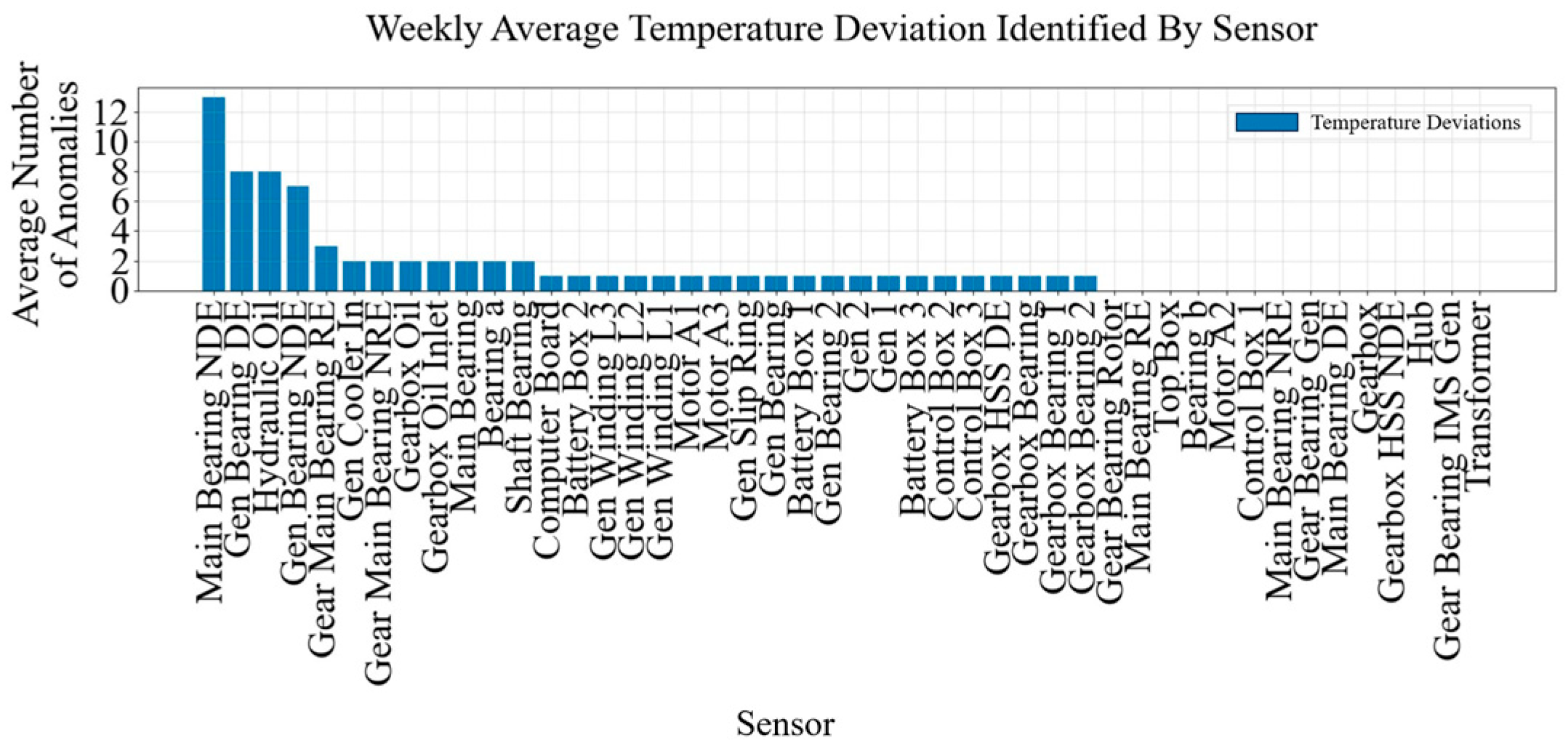
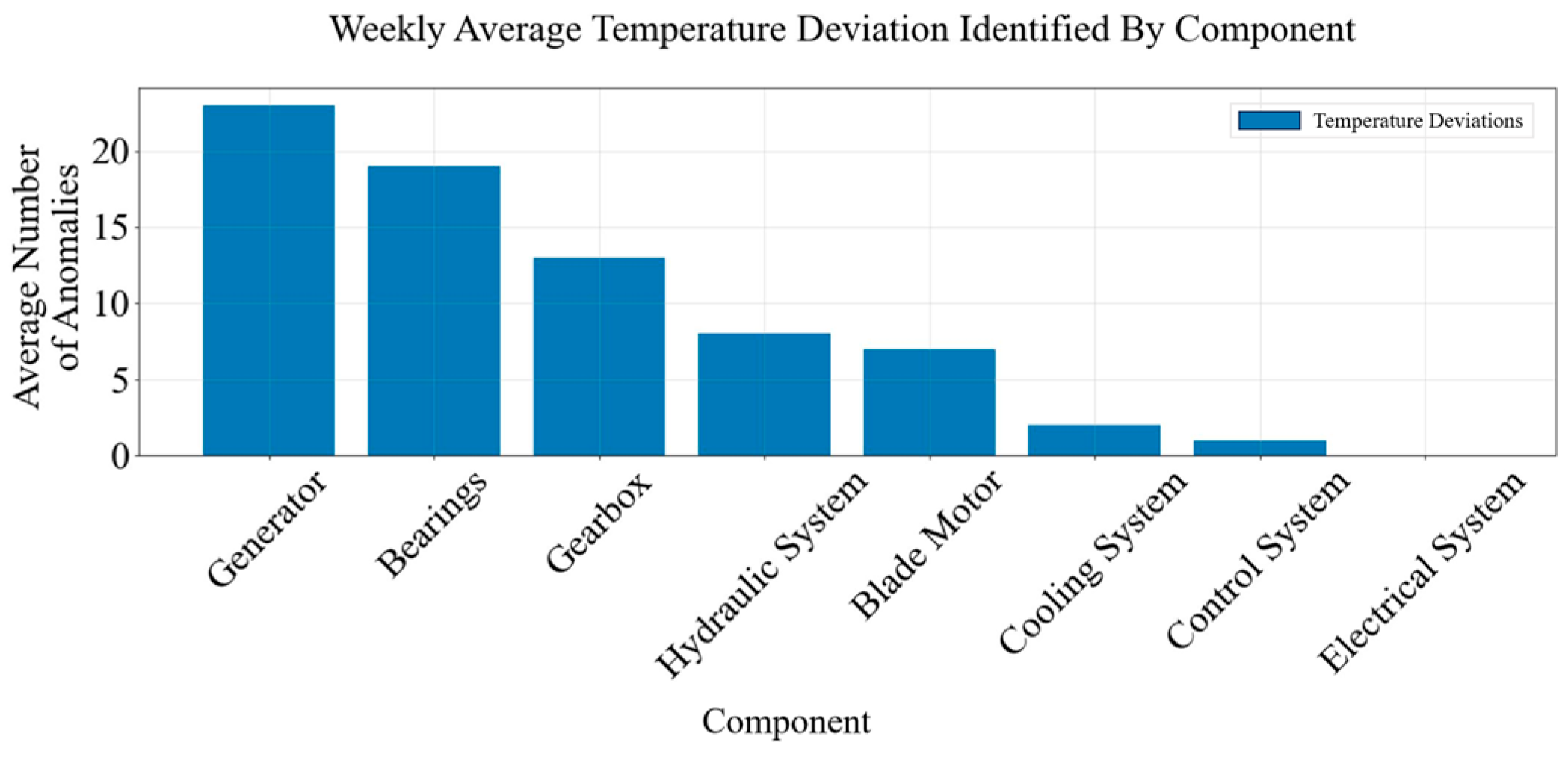
To address this, we establish a baseline for each turbine’s signals under normal operation and employ an EWMA control chart to flag significant deviations. After a series of tests, the results presented use a smoothing parameter $\lambda$ set to 0.7 and a weighting coefficient $k=6$. These parameters allow for the identification of only critical cases. As temperatures increase gradually and several weeks can elapse before a failure occurs, the resampling parameter $\delta t$ was set to 7 days, resulting in time series of 1008 observations. This duration ensures the continuous observation of equipment in operation (wind speeds above 3 m/s) and a sufficiently long period to detect real over-temperature events. For shorter periods, some cases of deviation are caused by intraday fluctuations in certain wind sectors. Finally, the time series were filtered by turbine, keeping only the observations where temperatures are above 30 degrees Celsius, ensuring a statistic calculated on equipment during operational periods. Discontinuities in the time series created by the filtering process are addressed during the calculation of the EWMA statistic through forward-fill followed by backward-fill sequence (ffill → bfill) (this assumes that the equipment maintains a constant operational condition in the missing data period). Forward-fill propagates the most recent valid measurement, while backward-fill resolves isolated gaps at the beginning of a resampled window. This imputation does not infer turbine behavior during uncertain states; it merely stabilizes the EWMA recursion under the assumption of short-term thermal continuity, consistent with standard practices in industrial signal smoothing and condition monitoring. For simplicity, each site represents a geographic zone, and no site grouping was performed at this level. An alert is raised only when the EWMA statistic crosses control limits, indicating an anomaly in the turbine’s behavior. To avoid spurious alerts, we enforced an alert persistence rule: an anomaly must persist for multiple consecutive readings ($>3·\delta t$) before it is reported. The output of OpS-EWMA is an anomaly score per turbine that triggers an alarm when sustained high. For the 3 months of data analyzed, over 98 turbines with temperature overhitting components were identified (Figure 2 and Figure 3).

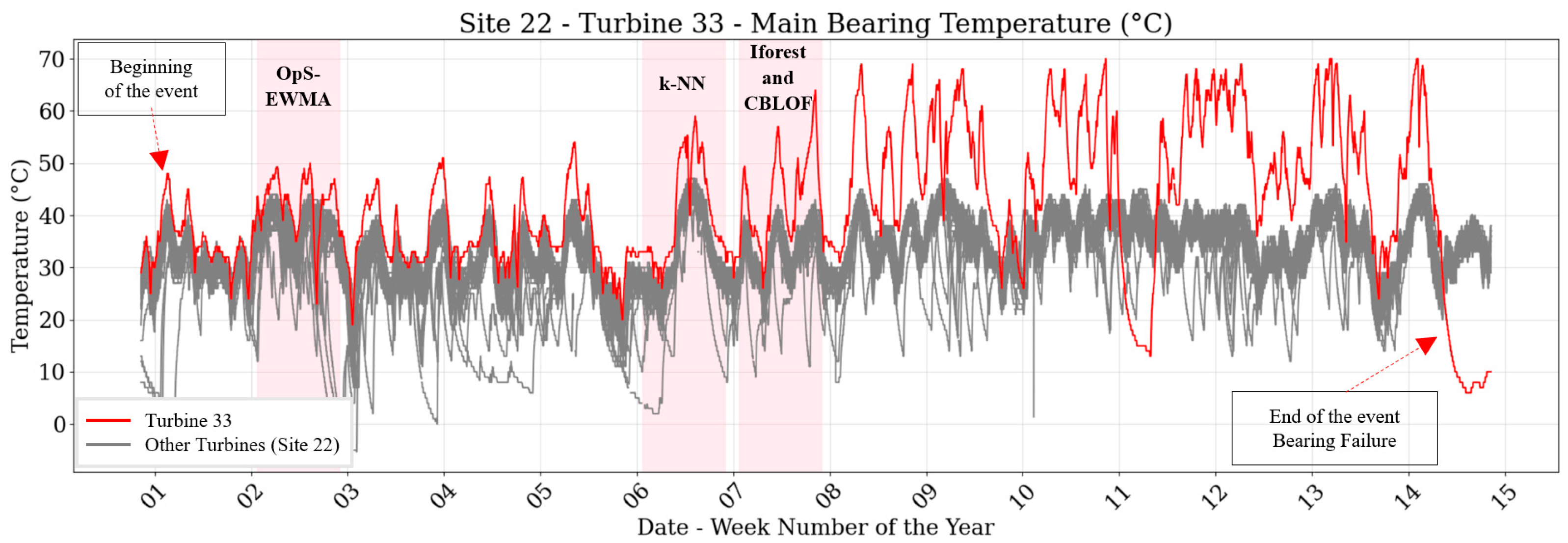
We benchmarked our proposed approach against three widely used anomaly detection methods: k-Nearest Neighbors (k-NN), Isolation Forest (IForest), and Cluster-Based Local Outlier Factor (CBLOF). To ensure comparability, input features were limited to wind speed, power, and component temperature, and data were normalized. Each method produced binary outputs (0 = normal, 1 = abnormal), resampled weekly (1008 observations); a week was considered abnormal if more than 50% of observations were flagged. This process generated OpS-Matrix equivalents for cross-method comparison. All baseline models required tuning of a parameter (neighbors, trees, clusters), which is difficult without labeled data; we used default settings from the PyOD library (K-NN with contamination = 0.1, n_neighbors = 5, method = “largest”, radius = 1.0 and metric = “minkowski”; IForest with n_estimators = 100, max_samples = “auto”, contamination = 0.1 and max_features = 1; and CBLOF with n_clusters = 8, contamination = 0.1, α = 0.9 and β = 5). A moving average of temperature was also included to improve performance. Results indicated broadly similar detection rates across methods, but our approach detected progressive deviations earlier (Figure 4).

A domain expert validated the anomalies identified by our method, noting that several non-isolated issues had escaped operator detection system. The methods, however, differ in their ability to capture isolated anomalies—short events (< seven days, based on the resampling frequency) detected by alarm systems and resolved through operator interventions. Excluding these cases, all four approaches detect a comparable range of anomalies [23]. OpS-EWMA identifies several additional events, mainly due to: (i) the limited three-month analysis period, with one-third of deviation appearing near its end, too early for other methods to capture; and (ii) the fixed $k$ parameter, which may not be optimal and would requires manual tuning per component type and turbine type—a key shortcoming of these approaches.

The baseline detectors (k-NN, IForest, CBLOF) were intentionally evaluated using their default PyOD hyperparameters. The goal of the comparison is to evaluate performance in a realistic zero-tuning deployment across thousands of heterogeneous turbines. Optimizing unsupervised detectors for each sensor or equipment would require thousands of subsystem-specific models and contradict the fleet-level objective. Similarly, the residual EWMA module operates with a single global parameter set ($\lambda$, $k$, $\delta t$, $\epsilon$ and $R_0$) without per-component tuning. Under these uniform conditions OpS-EWMA (and in particular its LLM-augmented variant) consistently outperformed the zero-tuning baselines, demonstrating superior robustness and practicality. Deep-learning detectors such as TCN-VAE, LSTM-VAE, GAN or Transformer-AD were excluded because they require fault-rich training data, extensive hyperparameter tuning and hardware resources that preclude their deployment at fleet scale.

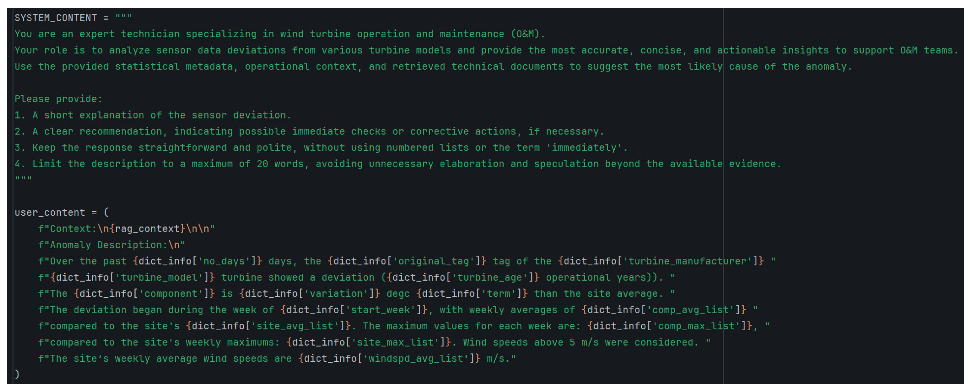
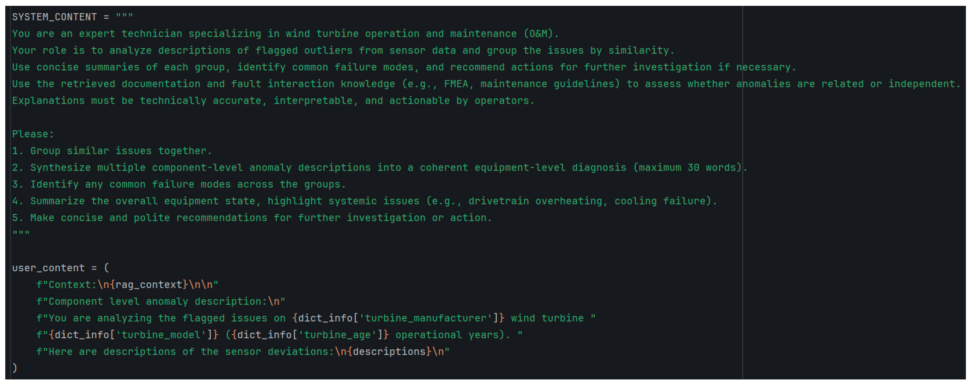
Following this validation, we structure the prompts for Phases I and II. Several configurations of the system content and user content were tested and analyzed before finalizing the structure presented below (Figure 5 and Figure 6). This prompt design forms the core of the framework: in a prompt-based architecture, the way prompts are structured has a decisive impact on the quality of the outputs.

The system content defines the role of the model, and the user content integrates two elements:

• The “rag_context”: is constructed using LangChain’s ingestion and retrieval pipeline. Documents (technical manuals, maintenance logs, and fault databases) are ingested with DirectoryLoader and split into manageable chunks using RecursiveCharacterTextSplitter. Each chunk is embedded into a dense vector representation with OpenAIEmbeddings, and the resulting embeddings are indexed in a FAISS vector store. At runtime, the anomaly description is converted into the same embedding space and used to query FAISS for the most relevant passages, which are then appended to the user prompt.
• The “dict_info” dictionary containing anomaly metadata: the number of days since detection (via OpS-EWMA), the original sensor tag, turbine manufacturer/model/age, component affected, and the variation compared to site averages. Weekly averages and maxima (component vs. site) and average wind speeds are also included (operating condition), aligned with the 7-day resampling used for the OpS-Matrix.

In phase II, the system content again defines the diagnostic role, while the user content begins with rag_context at the equipment level, enriched with manufacturer, model, and age information. It then incorporates the component-level explanations produced in Phase I, enabling the model to synthesize anomalies across subsystems and provide an equipment-level diagnostic. Once assembled, the system and user prompts (containing rag_context and dict_info) are sent to the OpenAI API for reasoning and explanation generation. In this design, LangChain handles the knowledge ingestion and retrieval pipeline, while the OpenAI API is used only for prompting the LLM—keeping the retrieval layer independent and adaptable.

4.1. Equipment Level Diagnostics and Severity Factor Calculation

Below, we present an example of the Phase I and Phase II model outputs (

Table 6. Example of Phase I and Phase II LLM assistant output.

Phase I—Component Level Analysis Output	Phase II—Equipment Level Diagnostics
1. 2.

). For confidentiality reasons, site names, time periods, turbine manufacturer, and model identifiers have been anonymized. Note also that we were limited on the documentation available for RAG. No maintenance records or FMEA were available. Only part of failure mode and technical manuals were used for phase I and some equipment operation manuals for phase II. An illustrative example of Phases I and II is provided in the following table. Phase II not only correlates anomalies into a systemic diagnosis but also reduces operator workload by consolidating two separate sensor checks into a single targeted inspection of the cooling system.

At the equipment level, the criticality state labels were computed using the formulas presented in the methodology section with equal weighting between the statistical and semantic score (${\lambda }_1={\lambda }_2={\displaystyle \frac{1}{4}}, {\lambda }_3={\displaystyle \frac{1}{2}}$). This process successfully generated the OpS-Vector at seven-day intervals (14 vectors, one per week), resulting in 24 validated equipment anomalies where more than two components deviated simultaneously (Figure 7). All cases received a semantic score of $I_{semantic}=0.33$ because the diagnostic texts consistently contained severity terms like “overheating” or “abnormal condition”, which belong to the Critical fault category (+1/3). None of the Phase II outputs contained urgent-action keywords (“immediate action”, “urgent repair”) or manufacturer/historical references (“OEM alert”, “historical failure mode”), so $S_i=0.33,{\mathrm{W}}_{\mathrm{i}}=0$ for all cases. The statistical score $I_{stat}$, on the other hand, varies across cases as a function of both the deviation amplitude and its duration.

The weights were not selected to represent an optimal configuration but instead reflect a balanced, domain-informed baseline that gives proportionally greater importance to semantic context. A full sensitivity study would require a much larger and more diverse dataset and direct collaboration with field engineers.

4.2. Fleet Level Diagnostics

Phase III extends the diagnostic pipeline to the fleet level by grouping turbines into homogeneous cohorts and reasoning over aggregated anomaly trends. In our implementation group formation was based on operational and engineering criteria such as manufacturers (Siemens, Vestas, GE), turbine model, derating category (e.g., curtailment profiles) and equipment age, all of which influence control logic, drivetrain design and thermal behavior. For each cohort, “dict_info” contains statistics summarizing the prevalence of each anomaly type normalized by group size, residual drifts from OpS-EWMA, distributional temperature metrics and patterns of anomaly duration and recurrence (Figure 8). These structured features were passed to the LLM, which reasoned about emerging fleet-level patterns. Such insights enable coordinated preventive interventions (e.g., lubrication campaigns) that are low-cost yet can prevent high-impact drivetrain failures. Phase III can also reveal operator-specific differences and systemic design issues when similar deviations occur across a large fraction of a cohort, guiding maintenance policies and manufacturer engagement.

We applied Phase III prompts to perform a fleet-level overview. For this exercise, turbines were grouped by manufacturer in order to identify recurring issues within specific turbine types across multiple sites. This revealed an important cross-site issue affecting one turbine type across multiple locations. The model diagnostics identified a progressive temperature increase across five gearbox bearings, suggesting lubrication as a preventive action. This was later confirmed by a technician, who noted that lubrication should have been performed earlier to avoid further escalation. Importantly, the model linked this issue to repeated shutdown events observed in similar turbine types (Figure 9), referencing documentation retrieved through the RAG process (internal reports). Validation showed that these turbines indeed a shutdown triggered by a temperature spike, which resulted in frequent restart cycles—over 20 shutdown/restart events within 24 h—completely missed by the alarm system.

Such undetected temperature-driven shutdowns pose significant risks: each emergency stop requires activation of the turbine’s mechanical brake, generating high stresses on the drivetrain. Repeated braking and restart cycles accelerate fatigue of the main bearing, couplings, and yaw/pitch mechanisms, and can propagate damage to connected subsystems like the gearbox and generator. Turbines are not designed to endure frequent hard stops, as this reduces component lifespan, increases maintenance costs, and threatens overall availability.

This case demonstrates that without an intelligent diagnostic layer, identifying the issue would require a time-consuming manual investigation—whereas our framework provides actionable insights within seconds.

4.3. Evaluation of Model Performance

Since the dataset was not originally labeled, we validated the model using an expert-in-the-loop approach. A total of 98 anomaly events were aggregated across all methods for which a complete chain of confirmation (sensor deviation → expert interpretation → technician verification) was available; when multiple detections occurred on the same equipment and within the same period, they were merged into a single event. This set was reviewed by a domain expert, who determined which were true positives and which were false alarms. Based on this validation, we assumed that the set of confirmed true positives represented the complete set of anomalies in the dataset. Obtaining multi-expert labels is challenging in industrial settings because confirmed failures are rare, maintenance logs are restricted and expert annotation is time-consuming. As a result, the present evaluation may underestimate the number of undetected anomalies (false negative rate), and slightly overestimate precision, yet it remains a consistent basis for comparing model performance. Although full ground-truth enumeration was not possible, complementary checks—including SCADA cross-validation, EWMA-trajectory stability analysis, threshold-sensitivity tests, and the separation of detection from LLM diagnosis—reduce the likelihood of substantial missed anomalies and help ensure that the reported metrics are not overly biased.

We compared our method against k-NN, Isolation Forest (IForest), and CBLOF. Performance was measured in terms of:

• Accuracy: proportion of correct predictions (both normal and anomalous).
• Precision: proportion of detected anomalies that were true positives.
• Recall: proportion of true anomalies that were successfully detected.
• F1-score: harmonic mean of precision and recall, balancing both.

Results (

Table 7. Average evaluation metrics over 5 runs: Comparison of three PyOD anomaly detection models (k-NN, IForest, CBLOF) with the proposed OpS-EWMA and its extended version OpS-EWMA–LLM (integrated with RAG, LangChain, and LLM diagnostics via the OpenAI API).

Metrics	Accuracy	Precision	Recall	F1 Score
K-NN	0.89	0.83	0.72	0.77
IForest	0.91	0.89	0.74	0.81
CBLOF	0.91	0.86	0.80	0.83
OpS-EWMA	0.94	0.93	0.83	0.88
OpS-EWMA-LLM	0.97	0.96	0.93	0.95

) show that incorporating the RAG with LLM reduces false positives through the criticality scoring step (which integrates semantic cues). Specifically, if an anomaly was triggered by OpS-EWMA but subsequently classified as Normal by the criticality layer, the event could be considered as normal (depending on scoring)—increasing precision by 3%. This aligns with the findings of the RAAD-LLM framework, which reported a 5% precision gain when applying RAG to their use-case dataset. Accuracy was already close to its maximum, as expected for state-of-the-art models in time-series anomaly detection, with only marginal improvement observed over baseline OpS-EWMA. Interpretation remains challenging given the unbalanced nature of the dataset, where most turbines operated normally (98 confirmed anomalies out of 1997 cases, representing fewer than 5% of the equipment in the dataset). OpS-EWMA combined with LLM diagnostics proved more sensitive to true positives, yielding a 10% recall improvement, consistent with RAAD-LLM results (23% recall improvement using RAG).

In summary, the case study demonstrates that integrating OpS-EWMA with LLM-based diagnostics and RAG improves anomaly detection and interpretation in real-world wind turbine data, yielding measurable gains in precision, recall, and F1-score. Regarding LLM accuracy, it is important to clarify that the objective of this work is not to evaluate the diagnostic performance of the LLM in isolation (e.g., through expert scoring, top-k agreement, or semantic similarity), but rather to quantify the end-to-end impact of incorporating semantic reasoning into the anomaly-detection pipeline; accordingly, LLM diagnostic consistency is captured indirectly through the semantic scoring layer, which influences the final classification. One of the next steps will be to extend the framework in a model-agnostic manner by benchmarking the outputs of different anomaly detection models to enhance robustness and accuracy, while in parallel working to gain access to larger datasets that could be released alongside an open-source Python implementation of the framework (Python 3.14), thereby providing a benchmark for the community and lowering barriers to reproducibility and adoption in the energy sector.

5. Conclusions

This study presented a unified framework, OpS-EWMA-LLM, that combines residual-based statistical process control with LLM diagnostics enhanced by RAG, hierarchical multi-phase prompting, and semantic scoring. The proposed approach is distinct from SPC–LLM (e.g., AAD-LLM/RAAD-LLM) or RAG-based diagnostic systems (e.g., RAG-GPT, HybridRAG, LLM + KG frameworks), which treat anomaly detection and explanation as separate stages or rely on LLMs as classifiers. In contrast, OpS-EWMA-LLM explicitly integrates fleet-normalized statistical deviation structures that guide and constrain hierarchical LLM reasoning within a single, tightly coupled pipeline.

Applied to SCADA data from almost 2000 wind turbines, the framework was evaluated under a strict zero-tuning strategy, in which all comparative methods were deployed using selected default parameter settings, without component-specific calibration. Under these conditions, OpS-EWMA-LLM outperformed baseline anomaly detection methods, consistently identifying incipient faults and producing human-understandable explanations, with critical deviations detected up to two weeks earlier than competing approaches. Such lead time is operationally valuable, as it allows operators to plan maintenance interventions, allocate resources, and mitigate risks before failures escalate. From an operational standpoint, the framework remains lightweight, as residual EWMA detection executes continuously on CPU with negligible computational overhead, and LLM inference is triggered only for a small subset of statistically significant events. To the best of our knowledge, this work represents one of the first approaches to address large-scale, heterogeneous equipment fleets using a computationally efficient and fully zero-tuning methodology for MVTS data.

The novelty of our methodology lies in its hybrid design: statistical detection ensures sensitivity and generalizability across heterogeneous fleets, while LLM-based reasoning enriches each alert with domain-grounded insights, supported by RAG to reduce hallucinations and increase traceability. The decision layer that fuses statistical severity with semantic cues produces interpretable criticality labels (Normal, Warning, Critical), thereby bridging quantitative anomaly evidence with qualitative operational knowledge. This dual-scoring logic offers a transparent and scalable means of building trust in AI-driven diagnostics. The relative influence of statistical detection and semantic interpretation is explicitly controlled through tunable weighting coefficients (${\lambda }_1$–${\lambda }_3$), ensuring that statistical evidence remains the primary driver of criticality while allowing semantic reasoning to refine interpretation when sufficient contextual evidence is available. Additionally, the semantic severity is computed using a transparent, fixed three-level keyword ontology derived from technical documentation and field reports, providing reproducible and interpretable diagnostic reasoning.

By reducing false alarms and enabling early identification of incipient faults, the proposed framework supports infrastructure sustainability beyond improved operational efficiency. Life-cycle assessments show that manufacturing and transporting a single gearbox or large bearing assembly emit approximately 25–60 t CO₂-eq, while crane mobilization adds 3–8 t CO₂-eq and the loss of 3–7 days of renewable generation (150–400 MWh) equates to 45–200 t CO₂-eq under typical OECD grid intensities. Preventing a single major drivetrain failure can therefore avoid roughly 70–250 t CO₂-eq when embodied emissions, logistic operations and lost renewable output are combined. Even minor interventions, such as avoiding a bearing replacement, yield meaningful emission and material savings [70]. These benefits align with UN Sustainable Development Goals: SDG 7 (Affordable and Clean Energy) by increasing renewable energy availability; SDG 9 (Industry, Innovation and Infrastructure) through AI-enabled reliability; SDG 12 (Responsible Consumption and Production) by extending component lifetimes; and SDG 13 (Climate Action) via avoiding greenhouse-gas emissions.

Looking forward, several avenues for development remain. First, constructing a historical case base by applying the framework to archived datasets will expand the diagnostic knowledge repository and support continual learning. Second, implementing a rolling window of recent data will enable real-time monitoring while filtering for active cases at a given time t, ensuring timely and actionable outputs. Third, scaling to fleet-wide deployment promises a practical solution for continuous anomaly detection and diagnostics in industrial operations. Upcoming efforts will further consolidate the framework, and a forthcoming paper will extend the methodology to transformer fleets, benchmarking performance against industry standards, while parallel initiatives aim to integrate additional datasets for broader cross-asset validation. We will also demonstrate how OpS-EWMA-LLM can further strengthen resilience assessment of electrical grids by constructing a knowledge base of critical operational states observed during extreme weather events. This will enable the development of data-driven mitigation strategies that enhance grid adaptability and recoverability, aligning the framework with the broader sustainability agenda for resilient and low-carbon energy systems.

We invite collaboration from researchers and practitioners interested in advancing explainable and multimodal diagnostic systems. Joint development of the framework—through shared datasets, domain expertise, or deployment partnerships—will accelerate progress toward reliable, real-time, and scalable solutions for condition monitoring across renewable energy and other critical infrastructure sectors.

References

1. Kaced, R.; Kouadri, A.; Baiche, K.; Bensmail, A. Multivariate nuisance alarm management in chemical processes. J. Loss Prev. Process Ind. 2021, 72, 104548. [Google Scholar] [CrossRef]
2. Zhao, J.; Huang, X.; Gao, Y.; Zhang, J.; Su, B.; Dong, Z. Research on machine learning-based correlation analysis method for power equipment alarms. In Proceedings of the 2022 International Conference on Informatics, Networking and Computing (ICINC), Nanjing, China, 14–16 October 2022. [Google Scholar] [CrossRef]
3. Shirshahi, A.; Aliyari-Shoorehdeli, M. Diagnosing root causes of faults based on alarm flood classification using transfer entropy and multi-sensor fusion approaches. Process Saf. Environ. Prot. 2024, 181, 469–479. [Google Scholar] [CrossRef]
4. Wang, J.; Yang, F.; Chen, T.; Shah, S.L. An Overview of Industrial Alarm Systems: Main Causes for Alarm Overloading, Research Status, and Open Problems. IEEE Trans. Autom. Sci. Eng. 2016, 13, 1045–1061. [Google Scholar] [CrossRef]
5. Lucke, M.; Chioua, M.; Grimholt, C.; Hollender, M.; Thornhill, N.F. Integration of alarm design in fault detection and diagnosis through alarm-range normalization. Control. Eng. Pract. 2020, 98, 104388. [Google Scholar] [CrossRef]
6. Lucke, M.; Chioua, M.; Grimholt, C.; Hollender, M.; Thornhill, N.F. Advances in alarm data analysis with a practical application to online alarm flood classification. J. Process Control. 2019, 79, 56–71. [Google Scholar] [CrossRef]
7. Leahy, K.; Gallagher, C.; O’Donovan, P.; O’Sullivan, D.T.J. Cluster analysis of wind turbine alarms for characterising and classifying stoppages. IET Renew. Power Gener. 2018, 12, 1146–1154. [Google Scholar] [CrossRef]
8. Kevin, L.; Colm, G.; Peter, O.D.; Ken, B.; Dominic, T.J.O.S. A Robust Prescriptive Framework and Performance Metric for Diagnosing and Predicting Wind Turbine Faults Based on SCADA and Alarms Data with Case Study. Energies 2018, 11, 1738. [Google Scholar] [CrossRef]
9. Abid, A.; Khan, M.T.; Iqbal, J. A review on fault detection and diagnosis techniques: Basics and beyond. Artif. Intell. Rev. 2021, 54, 3639–3664. [Google Scholar] [CrossRef]
10. Ju, Y.; Tian, X.; Liu, H.; Ma, L. Fault detection of networked dynamical systems: A survey of trends and techniques. Int. J. Syst. Sci. 2021, 52, 3390–3409. [Google Scholar] [CrossRef]
11. Garg, A.; Zhang, W.; Samaran, J.; Savitha, R.; Foo, C.S. An Evaluation of Anomaly Detection and Diagnosis in Multivariate Time Series. IEEE Trans. Neural Netw. Learn. Syst. 2022, 33, 2508–2517. [Google Scholar] [CrossRef] [PubMed]
12. Preciado-Grijalva, A.; Iza-Teran, V.R. Anomaly Detection of Wind Turbine Time Series using Variational Recurrent Autoencoders. arXiv 2021, arXiv:2112.02468. [Google Scholar] [CrossRef]
13. Chen, W.; Zhou, H.; Cheng, L.; Xia, M. Condition Monitoring and Anomaly Detection of Wind Turbines Using Temporal Convolutional Informer and Robust Dynamic Mahalanobis Distance. IEEE Trans. Instrum. Meas. 2023, 72, 3536914. [Google Scholar] [CrossRef]
14. Zhang, C.; Yang, T. Anomaly Detection for Wind Turbines Using Long Short-Term Memory-Based Variational Autoencoder Wasserstein Generation Adversarial Network under Semi-Supervised Training. Energies 2023, 16, 7008. [Google Scholar] [CrossRef]
15. Zwetsloot, I.M.; Jones-Farmer, L.A.; Woodall, W.H. Monitoring univariate processes using control charts: Some practical issues and advice. Qual. Eng. 2024, 36, 487–499. [Google Scholar] [CrossRef]
16. Ugaz, W.; Sánchez, I.; Alonso, A.s.M. Adaptive EWMA control charts with time-varying smoothing parameter. Int. J. Adv. Manuf. Technol. 2017, 93, 3847–3858. [Google Scholar] [CrossRef]
17. Khan, P.W.; Byun, Y.-C. A Review of machine learning techniques for wind turbine’s fault detection, diagnosis, and prognosis. Int. J. Green Energy 2024, 21, 771–786. [Google Scholar] [CrossRef]
18. Liu, J.; Yang, G.; Li, X.; Wang, Q.; He, Y.; Yang, X. Wind turbine anomaly detection based on SCADA: A deep autoencoder enhanced by fault instances. ISA Trans. 2023, 139, 586–605. [Google Scholar] [CrossRef]
19. Allal, Z.; Noura, H.N.; Vernier, F.; Salman, O.; Chahine, K. Wind turbine fault detection and identification using a two-tier machine learning framework. Intell. Syst. Appl. 2024, 22, 200372. [Google Scholar] [CrossRef]
20. Chen, X.; Lei, Y.; Li, Y.; Parkinson, S.; Li, X.; Liu, J.; Lu, F.; Wang, H.; Wang, Z.; Yang, B.; et al. Large Models for Machine Monitoring and Fault Diagnostics: Opportunities, Challenges and Future Direction. J. Dyn. Monit. Diagn. 2025, 4, 76–90. [Google Scholar] [CrossRef]
21. Gao, Y.; Xiong, Y.; Gao, X.; Jia, K.; Pan, J.; Bi, Y.; Dai, Y.; Sun, J.; Wang, M.; Wang, H. Retrieval-Augmented Generation for Large Language Models: A Survey. arXiv 2023, arXiv:2312.10997. [Google Scholar] [CrossRef]
22. Liu, Y.; Zhou, Y.; Liu, Y.; Xu, Z.; He, Y. Intelligent Fault Diagnosis for CNC Through the Integration of Large Language Models and Domain Knowledge Graphs. Engineering 2025, 53, 311–322. [Google Scholar] [CrossRef]
23. Chabane, B.; Komljenovic, D.; Abdul-Nour, G. Optimizing Performance of Equipment Fleets in Dynamic Environments: A Straightforward Approach to Detecting Shifts in Component Operational States. In Proceedings of the 2024 International Conference on Electrical, Computer and Energy Technologies, ICECET, Sydney, Australia, 25–27 July 2024; pp. 1–7. [Google Scholar] [CrossRef]
24. Tao, X.; Tula, A.; Chen, X. From prompt design to iterative generation: Leveraging LLMs in PSE applications. Comput. Chem. Eng. 2025, 202, 109282. [Google Scholar] [CrossRef]
25. Kandemir, E.; Hasan, A.; Kvamsdal, T.; Abdel-Afou Alaliyat, S. Predictive digital twin for wind energy systems: A literature review. Energy Inform. 2024, 7, 68. [Google Scholar] [CrossRef]
26. Liu, S.; Ren, S.; Jiang, H. Predictive maintenance of wind turbines based on digital twin technology. Energy Rep. 2023, 9, 1344–1352. [Google Scholar] [CrossRef]
27. Habbouche, H.; Amirat, Y.; Benbouzid, M. Leveraging Digital Twins and AI for Enhanced Gearbox Condition Monitoring in Wind Turbines: A Review. Appl. Sci. 2025, 15, 5725. [Google Scholar] [CrossRef]
28. Zhou, Y.; Zhou, J.; Cui, Q.; Wen, J.; Fei, X. Digital twin-driven online intelligent assessment of wind turbine gearbox. Wind. Energy 2024, 27, 797–815. [Google Scholar] [CrossRef]
29. Leon-Medina, J.X.; Tibaduiza, D.A.; Parés, N.; Pozo, F. Digital twin technology in wind turbine components: A review. Intell. Syst. Appl. 2025, 26, 200535. [Google Scholar] [CrossRef]
30. Zhong, D.; Xia, Z.; Zhu, Y.; Duan, J. Overview of predictive maintenance based on digital twin technology. Heliyon 2023, 9, e14534. [Google Scholar] [CrossRef]
31. Yang, T.; Pen, H.; Wang, Z.; Chang, C.S. Feature Knowledge Based Fault Detection of Induction Motors Through the Analysis of Stator Current Data. IEEE Trans. Instrum. Meas. 2016, 65, 549–558. [Google Scholar] [CrossRef]
32. Delgoshaei, P.; Delgoshaei, P.; Austin, M. Framework for Knowledge-Based Fault Detection and Diagnostics in Multi-Domain Systems: Application to HVAC Systems; Institute for Systems Research: College Park, MD, USA, 2017. [Google Scholar] [CrossRef]
33. Zhong, M.; Zhu, X.; Xue, T.; Zhang, L. An overview of recent advances in model-based event-triggered fault detection and estimation. Int. J. Syst. Sci. 2023, 54, 929–943. [Google Scholar] [CrossRef]
34. Isermann, R. Model-based fault-detection and diagnosis—Status and applications. Annu. Rev. Control 2005, 29, 71–85. [Google Scholar] [CrossRef]
35. Jieyang, P.; Kimmig, A.; Dongkun, W.; Niu, Z.; Zhi, F.; Jiahai, W.; Liu, X.; Ovtcharova, J. A systematic review of data-driven approaches to fault diagnosis and early warning. J. Intell. Manuf. 2023, 34, 3277–3304. [Google Scholar] [CrossRef]
36. Li, B.; Yang, Y. Data-Driven Optimal Distributed Fault Detection Based on Subspace Identification for Large-Scale Interconnected Systems. IEEE Trans. Ind. Inform. 2024, 20, 2497–2507. [Google Scholar] [CrossRef]
37. Abid, K.; Sayed Mouchaweh, M.; Cornez, L. Fault Prognostics for the Predictive Maintenance of Wind Turbines: State of the Art. In ECML PKDD 2018 Workshops; Springer International Publishing: Cham, Switzerland, 2019. [Google Scholar] [CrossRef]
38. Ahmed, I.; Dagnino, A.; Ding, Y. Unsupervised Anomaly Detection Based on Minimum Spanning Tree Approximated Distance Measures and Its Application to Hydropower Turbines. IEEE Trans. Autom. Sci. Eng. 2019, 16, 654–667. [Google Scholar] [CrossRef]
39. Lin, K.; Pan, J.; Xi, Y.; Wang, Z.; Jiang, J. Vibration anomaly detection of wind turbine based on temporal convolutional network and support vector data description. Eng. Struct. 2024, 306, 117848. [Google Scholar] [CrossRef]
40. Eugenio, B.; Luca, C.; Cristiana, D.; Luigi Gianpio Di, M. Explainable AI for Machine Fault Diagnosis: Understanding Features’ Contribution in Machine Learning Models for Industrial Condition Monitoring. Appl. Sci. 2023, 13, 2038. [Google Scholar] [CrossRef]
41. Lu, W.; Liliang, W.; Feng, L.; Zheng, Q. Clustering Analysis of Wind Turbine Alarm Sequences Based on Domain Knowledge-Fused Word2vec. Appl. Sci. 2023, 13, 10114. [Google Scholar] [CrossRef]
42. Raza, M.; Jahangir, Z.; Riaz, M.B.; Saeed, M.J.; Sattar, M.A. Industrial applications of large language models. Sci. Rep. 2025, 15, 13755. [Google Scholar] [CrossRef]
43. Maximilian, L. A Text-Based Predictive Maintenance Approach for Facility Management Requests Utilizing Association Rule Mining and Large Language Models. Mach. Learn. Knowl. Extr. 2024, 6, 233–258. [Google Scholar] [CrossRef]
44. Palma, G.; Cecchi, G.; Rizzo, A. Large Language Models for Predictive Maintenance in the Leather Tanning Industry: Multimodal Anomaly Detection in Compressors. Electronics 2025, 14, 2061. [Google Scholar] [CrossRef]
45. Park, J.; Atarashi, K.; Takeuchi, K.; Kashima, H. Emulating Retrieval Augmented Generation via Prompt Engineering for Enhanced Long Context Comprehension in LLMs. arXiv 2025, arXiv:2502.12462. [Google Scholar] [CrossRef]
46. Alsaif, K.M.; Albeshri, A.A.; Khemakhem, M.A.; Eassa, F.E. Multimodal Large Language Model-Based Fault Detection and Diagnosis in Context of Industry 4.0. Electronics 2024, 13, 4912. [Google Scholar] [CrossRef]
47. Mecklenburg, N.; Lin, Y.; Li, X.; Holstein, D.; Nunes, L.; Malvar, S.; Silva, B.; Chandra, R.; Aski, V.; Yannam, P.K.R.; et al. Injecting New Knowledge into Large Language Models via Supervised Fine-Tuning. arXiv 2024, arXiv:2404.00213. [Google Scholar] [CrossRef]
48. Heredia Álvaro, J.A.; Barreda, J.G. An advanced retrieval-augmented generation system for manufacturing quality control. Adv. Eng. Inform. 2025, 64, 103007. [Google Scholar] [CrossRef]
49. Xu, J.; Xu, Z.; Jiang, Z.; Chen, Z.; Luo, H.; Wang, Y.; Gui, W. Labeling-free RAG-enhanced LLM for intelligent fault diagnosis via reinforcement learning. Adv. Eng. Inform. 2026, 69, 103864. [Google Scholar] [CrossRef]
50. Xie, X.; Tang, X.; Gu, S.; Cui, L. An intelligent guided troubleshooting method for aircraft based on HybirdRAG. Sci. Rep. 2025, 15, 17752. [Google Scholar] [CrossRef]
51. Russell-Gilbert, A.; Mittal, S.; Rahimi, S.; Seale, M.; Jabour, J.; Arnold, T.; Church, J. RAAD-LLM: Adaptive Anomaly Detection Using LLMs and RAG Integration. arXiv 2025, arXiv:2503.02800. [Google Scholar] [CrossRef]
52. Jin, M.; Wen, Q.; Liang, Y.; Zhang, C.; Xue, S.; Wang, X.; Zhang, J.; Wang, Y.; Chen, H.; Li, X.; et al. Large Models for Time Series and Spatio-Temporal Data: A Survey and Outlook. arXiv 2023, arXiv:2310.10196. [Google Scholar] [CrossRef]
53. Jin, M.; Wang, S.; Ma, L.; Chu, Z.; Zhang, J.Y.; Shi, X.; Chen, P.-Y.; Liang, Y.; Li, Y.-F.; Pan, S.; et al. Time-LLM: Time Series Forecasting by Reprogramming Large Language Models. arXiv 2023, arXiv:2310.01728. [Google Scholar] [CrossRef]
54. Ansari, A.F.; Stella, L.; Turkmen, C.; Zhang, X.; Mercado, P.; Shen, H.; Shchur, O.; Rangapuram, S.S.; Arango, S.P.; Kapoor, S.; et al. Chronos: Learning the Language of Time Series. arXiv 2024, arXiv:2403.07815. [Google Scholar] [CrossRef]
55. Zhou, T.; Niu, P.; Wang, X.; Sun, L.; Jin, R. One Fits All:Power General Time Series Analysis by Pretrained LM. arXiv 2023, arXiv:2302.11939. [Google Scholar] [CrossRef]
56. Sun, C.; Li, H.; Li, Y.; Hong, S. TEST: Text Prototype Aligned Embedding to Activate LLM’s Ability for Time Series. arXiv 2023, arXiv:2308.08241. [Google Scholar] [CrossRef]
57. Chabane, B.; Komljenovic, D.; Abdul-Nour, G. Converging on human-centred industry, resilient processes, and sustainable outcomes in asset management frameworks. Environ. Syst. Decis. 2023, 43, 663–679. [Google Scholar] [CrossRef]
58. Harrou, F.; Bouyeddou, B.; Sun, Y. Sensor Fault Detection in Wind Turbines Using Machine Learning and Statistical Monitoring Chart. In Proceedings of the 2023 Prognostics and Health Management Conference (PHM), Salt Lake City, UT, USA, 28 October–2 November 2023; pp. 344–349. [Google Scholar] [CrossRef]
59. Haridy, S.; Wu, Z. Univariate and multivariate control charts for monitoring dynamic-behavior processes: A case study. J. Ind. Eng. Manag. 2009, 2, 464. [Google Scholar] [CrossRef]
60. Hartkopf, J.P.; Reh, L. Challenging golden standards in EWMA smoothing parameter calibration based on realized covariance measures. Financ. Res. Lett. 2023, 56, 104129. [Google Scholar] [CrossRef]
61. Areepong, Y.; Chananet, C. Optimal parameters of EWMA Control Chart for Seasonal and Non-Seasonal Moving Average Processes. J. Phys. Conf. Ser. 2021, 2014, 012005. [Google Scholar] [CrossRef]
62. Lucas, J.M.; Saccucci, M.S. Exponentially Weighted Moving Average Control Schemes: Properties and Enhancements. Technometrics 1990, 32, 1–12. [Google Scholar] [CrossRef]
63. Jones, L.A.; Champ, C.W.; Rigdon, S.E. The Performance of Exponentially Weighted Moving Average Charts With Estimated Parameters. Technometrics 2001, 43, 156–167. [Google Scholar] [CrossRef]
64. Harrou, F.; Sun, Y.; Hering, A.S.; Madakyaru, M.; Dairi, A. Statistical Process Monitoring Using Advanced Data-Driven and Deep Learning Approaches: Theory and Practical Applications; Elsevier: San Diego, CA, USA, 2020. [Google Scholar]
65. Cambron, P.; Tahan, A.; Masson, C.; Pelletier, F. Bearing temperature monitoring of a Wind Turbine using physics-based model. J. Qual. Maint. Eng. 2017, 23, 479–488. [Google Scholar] [CrossRef]
66. Harrou, F.; Sun, Y.; Dorbane, A.; Bouyeddou, B. Sensor fault detection in photovoltaic systems using ensemble learning-based statistical monitoring chart. In Proceedings of the 2023 11th International Conference on Smart Grid (icSmartGrid), Paris, France, 4–7 June 2023; pp. 1–6. [Google Scholar] [CrossRef]
67. Cambron, P.; Masson, C.; Tahan, A.; Pelletier, F. Control chart monitoring of wind turbine generators using the statistical inertia of a wind farm average. Renew. Energy 2018, 116, 88–98. [Google Scholar] [CrossRef]
68. Dhada, M.; Girolami, M.; Parlikad, A.K. Anomaly detection in a fleet of industrial assets with hierarchical statistical modeling. Data-Centric Eng. 2020, 1, e21. [Google Scholar] [CrossRef]
69. Hendrickx, K.; Meert, W.; Mollet, Y.; Gyselinck, J.; Cornelis, B.; Gryllias, K.; Davis, J. A general anomaly detection framework for fleet-based condition monitoring of machines. Mech. Syst. Signal Process. 2020, 139, 106585. [Google Scholar] [CrossRef]
70. Guezuraga, B.; Zauner, R.; Pölz, W. Life cycle assessment of two different 2 MW class wind turbines. Renew. Energy 2012, 37, 37–44. [Google Scholar] [CrossRef]
71. Plumley, C.; Takeuchi, R. Penmanshiel wind farm data (Version v3). Zenodo 2025. [Google Scholar] [CrossRef]
72. Plumley, C.; Takeuchi, R. Kelmarsh wind farm data (Version v4). Zenodo 2025. [Google Scholar] [CrossRef]
Figure 1. Integrated pipeline for multivariate time-series anomaly detection and LLM-assisted diagnostic.
Sustainability 18 00132 g001
Figure 2. Occurrence of anomalies per sensor.
Sustainability 18 00132 g002
Figure 3. Occurrence of anomalies per component.
Sustainability 18 00132 g003
Figure 4. Detection time comparison of main bearing anomaly across four methods—OpS-EWMA detected the anomaly in week 2, well before the 70 °C alarm threshold. By contrast, k-NN identified it only in week 6, IForest and CBLOF in week 7, while the alarm system failed to trigger until week 14—the same week the bearing failure occurred.
Sustainability 18 00132 g004
Figure 5. Phase I prompt structure.
Sustainability 18 00132 g005
Figure 6. Phase II prompt structure.
Sustainability 18 00132 g006
Figure 7. Criticality scores for 24 flagged turbines—consolidated into 12 anomaly types.
Sustainability 18 00132 g007
Figure 8. Phase III prompt structure.
Sustainability 18 00132 g008
Figure 9. Fleet-Level LLM diagnostic output identifying recurrent gearbox bearing overheating and shutdown events.
Sustainability 18 00132 g009