Abstract
Rapid economic development, accelerated urbanization, and agricultural modernization in eastern China have exacerbated pollution in rivers discharging into the sea, challenging regional ecological security and water resource sustainability. This study investigates ten main rivers in eastern China using monthly water quality and hydrological data from 2021 to 2023. Pollutant fluxes for permanganate index (), ammonia nitrogen (AN), total phosphorus (TP), and total nitrogen (TN) were calculated, and their temporal and spatial variations were analyzed using descriptive statistics, two-way analysis of variance (ANOVA), and principal component analysis (PCA). Results show significant spatial heterogeneity, with the Yangtze (YAR) and Pearl Rivers (PER) exhibiting the highest fluxes due to high basin runoff and intense human activities. Seasonal variations significantly affect , TP, and TN fluxes, with summer runoff and agricultural activities enhancing pollutant transport. Moreover, flood periods markedly increase pollutant fluxes compared to non-flood periods. PCA further reveals that the pollutant flux patterns of YAR and PER are clearly distinct from those of the other rivers, indicating the joint influence of geographic conditions and anthropogenic activities. This study provides quantitative evidence for regional water environment management and offers crucial guidance for developing sustainable, differentiated pollution control strategies.
1. Introduction
In recent years, the rapid economic development, accelerated urbanization, and advancement of agricultural modernization in China have led to increasingly severe river environmental issues in eastern coastal regions [1,2]. The major rivers discharging into the sea within the region not only provide abundant water resources but also directly affect coastal ecosystems and marine environments [3,4]. Nevertheless, as industrial and agricultural activities expand, nutrients such as nitrogen and phosphorus inevitably enter river systems, causing water quality to deteriorate progressively [5]. This degradation poses a severe challenge to regional ecological security and the sustainable utilization of water resources. The river water quality issue is increasingly serious, which not only threatens freshwater utilization, particularly for drinking water, but also risks causing substantial harm to marine ecosystems through riverine inputs [6,7,8]. The degradation of freshwater quality can substantially alter the ecological structure and function of rivers, lakes, and reservoirs, leading to ecosystem decline and water shortages that seriously hinder basin-wide sustainable development [9,10]. Consequently, characterizing the spatiotemporal variability of water quality in rivers discharging into the sea is essential for effective ecological management and pollution control. In-depth studies on this topic supply policymakers and environmental managers with critical scientific evidence to uphold ecological balance and ensure the long-term sustainability of water resources. Such insights are fundamental to devising targeted strategies for mitigating pollution in coastal river systems and preserving the integrity of freshwater ecosystems.
Over the past few years, many studies have employed various statistical analysis methods from different perspectives to explore the water quality conditions and spatio-temporal variation characteristics of rivers discharging into the sea. Prior investigations on this field has predominantly focused on the spatio-temporal analysis of pollutant concentrations. For example, Koch et al. [11] analyzed the characteristics of water quality over 21 years in a North-Eastern Germany lowland watershed, revealing overall improvements in surface water quality, with phosphorus concentrations and loads exhibiting variability across seasons. Mamun et al. [12] investigated the spatio-temporal characteristics of water quality and its influencing factors in the Geum River, discovering that total suspended solids, chlorophyll-a, TP, and chemical oxygen demand were higher in summer than in other seasons. Bu et al. [13] conducted an in-depth study on the spatio-temporal variation of water quality in the Jinshui River of the South Qinling Mts., China, revealing significant temporal and spatial differences in pollutants, with water quality gradually deteriorating from the headwater to downstream. Moreover, many studies have demonstrated the spatio-temporal heterogeneity of pollutants such as TP and TN across different rivers or basins [14,15,16,17,18]. In addition, several scholars have applied cutting-edge statistical or computational methods to showcase the dynamic spatio-temporal features of river water quality. Chang et al. [19] proposed a systematical modeling approach based on dynamic neural networks combined with three refined statistical methods, and investigated a decade of seasonal water quality data collected from seven monitoring stations along the Dahan River in Taiwan, China. They found that the proposed model effectively captured key characteristics of TP concentration dynamics. Wang et al. [20] employed a combination of the Mann-Kendall test, clustering analysis, self-organizing map, the Boruta algorithm, and positive matrix factorization to comprehensively assess the interactions between land use types and various water quality parameters in the Huaihe River basin, China, revealing that these interactions vary with the seasons. Currently, most studies still focus on the spatio-temporal changes in pollutant concentrations in rivers [21,22]; however, single concentration data are insufficient to fully reflect the transport and diffusion processes of pollutants within river systems. In contrast, pollutant flux can more directly reveal the spatio-temporal distribution and transport characteristics of pollutants, offering higher scientific value for evaluating river water environments. This is particularly important in regions where hydrological conditions, climate change, and the intensity of human activities vary significantly in space, making a systematic study of the spatio-temporal variations in pollutant flux is an urgent scientific issue.
This paper focuses on ten major rivers in eastern China that discharge into the sea, which are distributed across seven distinct river basins and each exhibit unique characteristics. For example, between 2021 and 2023, the annual runoff of the Yangtze River exceeded 800 billion cubic meters, which resulted in significantly higher pollutant fluxes compared to other rivers. In addition, seasonal variations in runoff also contribute to fluctuations in pollutant fluxes. For instance, the Haihe River experiences much higher runoff during the summer and autumn compared to the winter and spring, which leads to notably elevated pollutant fluxes in the summer season. The significant differences in hydrological properties, precipitation patterns, temperature variations, and levels of economic activity among these basins result in complex and varied mechanisms governing the generation, transport, and diffusion of pollutants. To address this complexity, the study utilizes monthly monitoring data from 2021 to 2023 to calculate pollutant fluxes, including the , AN, TP, TN, and employs descriptive statistics, two-way ANOVA, and PCA to systematically investigate the spatio-temporal variations of pollutant fluxes in these rivers under different seasonal conditions as well as during flood and non-flood periods. The primary innovations of this work include: (1) a detailed examination of current water quality status in eastern Chinese rivers discharging into the sea, with an in-depth exploration of the spatial heterogeneity of river pollutant fluxes; (2) an investigation into the temporal heterogeneity of pollutant fluxes from two perspectives, namely seasonal variations and differences between flood and non-flood seasons, provides essential knowledge for improving the sustainability of river ecosystems both seasonally and under different flow regimes; (3) an analysis of the spatio-temporal characteristics of pollutants in eastern Chinese rivers that not only has significant implications for improving riverine ecological environments but also offers a reference for the management of river water quality on a global scale.
2. Materials and Methods
2.1. Study Area
This research is centered on the eastern region of mainland China. China is located in East Asia, with a longitude of E to E and a latitude of N to N. This study encompasses seven major river basins in eastern China. From these basins, we selected ten principal rivers for detailed analysis. The specific rivers and their respective basins have been summarized in Table 1. Data on river basin divisions were sourced from the Resource and Environmental Science Data Platform (https://www.resdc.cn/data.aspx?DATAID=141, accessed on 26 April 2025), provided by the Institute of Geographic Sciences and Natural Resources Research, Chinese Academy of Sciences. The coordinate system used was GCS_WGS_1984. The spatial distribution of hydrological stations and water quality stations for each river is systematically presented in Figure 1 and Table 1. The selected basins exhibit significant heterogeneity in hydrological regimes, climatic conditions, and socioeconomic development levels, which may lead to spatial variations in pollutant fluxes across different rivers.

Table 1.
Informations of rivers and coordinates of sampling stations.
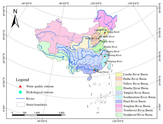
Figure 1.
Map of the sampling stations.
2.2. Data Sources
The water quality data for this study were sourced from China National Environmental Monitoring Centre (available at https://www.cnemc.cn, accessed on 16 February 2024). The pollutant concentration data were collected in accordance with the Environmental Quality Standards for Surface Water (GB 3838-2002). The hydrological data were obtained from China River Sediment Bulletin, which is published by Ministry of Water Resources of the People’s Republic of China (available at http://www.mwr.gov.cn, accessed on 2 May 2024). The analyzed dataset comprises monthly records spanning a three-year period from 2021 to 2023. Pollutant flux calculation [23,24] is defined as:
where F is the monthly pollutant flux (t), C is the monthly mean pollutant concentration (mg/L), and Q is the monthly runoff ( ).
To characterize season variations in pollutant fluxes, we established a standardized seasonal framework with spring spanning from March to May, summer from June to August, autumn from September to November, and winter from December to February. River-specific flood seasons were designated according to hydrological patterns: the flood season of YAR is from May to October, YER is from June to October, PER is from April to September, HUAI, LUAN, HAI, LIAO and HUN are from June to September, QTR and MJR are from May to September. This basin-specific setting of flood seasons accounts for heterogeneous precipitation regimes, snowmelt cycles, and water management practices across different geographical regions, enabling systematic comparison of pollutant fluxes dynamics between flood season and non-flood season.
2.3. Statistical Method
Data processing and analysis were conducted using the R 4.3.2 programming language. In the data pre-processing stage, missing values within each river dataset were initially imputed using linear interpolation. Subsequently, pollutant fluxes in every river were calculated according to the method described in (1). During the analysis phase, descriptive statistics of pollutant fluxes, including the minimum, maximum, median, mean, standard deviation, skewness, and kurtosis, were computed. Violin plots were then utilized to illustrate the distribution of pollutant fluxes for different pollutants across various rivers and years. A two-way ANOVA was subsequently performed to investigate the differences in pollutant levels associated with seasonal variations and river characteristics, as well as between flood and non-flood periods across rivers. Pairwise comparisons were carried out using boxplots and mean bar charts, accompanied by Tukey HSD tests. Finally, PCA was applied to explore the patterns of pollutant fluxes during different seasons and between flood season and non-flood season. The study made use of R packages including zoo 1.8.12 [25], pastecs 1.4.2 [26], tidyplots 0.2.2 [27], ggplot2 3.5.1 [28], FactoMineR 2.11 [29] and factoextra 1.0.7 [30].
3. Results
3.1. Basic Descriptive Statistics for Pollutant Fluxes
Since the pollutant flux data analyzed in this study were derived from river runoff measurements, short-term events such as rainfall and flooding can have a significant impact on the flux values. Therefore, to better capture the hydrological characteristics of each river, we plotted the time series of river runoff in Figure 2.
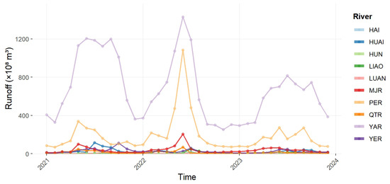
Figure 2.
Time series plot of runoff.
The fundamental descriptive statistical analysis of pollutant fluxes in ten main rivers discharging into the sea in eastern Chinese elucidates their overall distribution patterns, forming the foundation for subsequent spatio-temporal characterization. Table 2 presents comprehensive univariate descriptive statistics for four pollutant fluxes, including minimum, maximum, median, mean, standard deviation, skewness, and kurtosis. The statistical results demonstrate substantial variations in pollutant fluxes. Wide ranges between minimum and maximum values, accompanied by large standard deviations (1.47 × – × ), suggest possible temporal variations and possible spatial variations in pollutant fluxes between different rivers. All pollutant fluxes show high median and mean values, with means systematically higher than medians. This pattern, reinforced by positive skewness values (3.35–5.14), indicates right-skewed distributions with potential high-value outliers. Furthermore, the leptokurtic nature of distributions (kurtosis > 0) demonstrates pronounced peakness compared to normal distributions, indicating higher probabilities of extreme values.
Table 2.
Univariate descriptive statistical analysis of pollutant fluxes.
Figure 3 presents violin plots illustrating the spatio-temporal distribution of four pollutant fluxes across different rivers and years. Analysis of Figure 3 reveals several notable findings. All four pollutant fluxes are significantly higher in YAR compared to other rivers. PER maintained secondary pollutant flux levels following YAR during the 2021–2023 observation period. PER exhibited interannual variability, with 2022 showing higher pollutant fluxes across all four pollutants and the presence of outlier data points compared to 2021 and 2023. Comparative analysis identified similar pollutant flux distribution patterns between LIAO, HUN, LUAN, and HAI during 2022 to 2023; however, HAI displayed moderately higher fluxes across all four pollutants relative to the other three rivers in 2021. Pollutant fluxes demonstrated variations, with and TN exhibiting considerably higher values than AN and TP across all rivers.
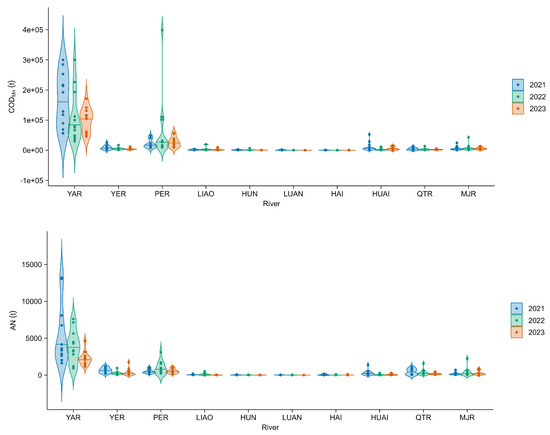
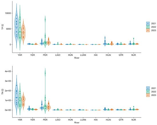
Figure 3.
Violin plots of pollutant fluxes across different rivers and years.
3.2. Analysis of Variance for Season and River Factors
Table 3 presents the results of a two-way ANOVA for the four pollutants across the factors of season and river. The results in Table 3 indicate that the effects of both season and river on pollutant fluxes are significantly different.
Table 3.
Two-way ANOVA results on pollutant fluxes among seasons and rivers.
Regarding the seasonal effect, season has a significant impact on the fluxes of , TP, and TN (p-value < 0.001), while its effect on AN is only marginally significant (F-statistic = 2.626, p-value = 0.051); Regarding the river effect, the river factor shows highly significant effects on all pollutant fluxes (p-value < 0.001), indicating marked spatial differences in pollutant fluxes among the different rivers. Notably, the influence of the river factor is most significant for TP (F-statistic = 151.039), followed by TN (F-statistic = 72.912) and (F-statistic = 65.088); Regarding the interaction effect, the interaction between season and river significantly affects the fluxes of , TP, and TN (p-value < 0.001), but not AN (F-statistic = 0.493, p-value = 0.985), suggesting that the spatio-temporal variation of AN is primarily driven by the independent effects of season or river.
Figure 4 presents box plots comparing the pollutant fluxes among different rivers across seasons, along with pairwise comparisons. In spring, significant differences (p-value < 0.001) were observed in the fluxes of , AN, TP, and TN between YAR and the other rivers. Similarly, the fluxes of , AN, TP, and TN in PER were significantly different (p-value < 0.05) compared to YAR, LIAO, HUN, LUAN, and HAI. Moreover, significant differences (p-value < 0.05) in and TN fluxes were found between PER and YER; significant differences (p-value < 0.05) in , AN, and TN fluxes were observed between PER and HUAI; and significant differences (p-value < 0.05) in and TN fluxes were detected between PER and QTR. Finally, the TN flux in PER differed significantly from that in MJR (p-value < 0.001).
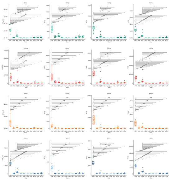
Figure 4.
Box plots and Tukey HSD test results of pollutant fluxes between different rivers. *: p-value < 0.05; **: p-value < 0.01; ***: p-value < 0.001.
In summer, YAR continues to exhibit highly significant differences (p-value < 0.001) in the fluxes of , AN, TP, and TN compared to the other nine rivers. In addition, the PER shows significant differences (p-value < 0.05) in and TN fluxes relative to the other rivers, although no significant difference in TP flux is observed between PER and MLR. Furthermore, among the nine rivers other than YAR, no significant pairwise differences in AN flux are found (p-value > 0.05).
In autumn, it was observed that YAR exhibited significant differences in the fluxes of , AN, TP, and TN compared to the other nine rivers (p-value < 0.05). However, among the nine rivers excluding YAR, no significant differences in pollutant fluxes were detected (p-value > 0.05).
In winter, YAR continues to demonstrate extremely significant differences (p-value < 0.001) in the fluxes of , AN, TP, and TN compared to the other nine rivers. Similarly, PER exhibits relatively significant differences (p-value < 0.001) in the fluxes of , AN, TP, and TN relative to the other nine rivers. Furthermore, significant differences (p-value < 0.05) in TP flux are observed between PER and YAR, LUAN, HAI. However, among the nine rivers excluding the Yangtze, no significant differences in AN flux were detected (p-value > 0.05).
Figure 5, Figure 6, Figure 7 and Figure 8 reports the pairwise comparison results of the four pollutant fluxes across different seasons for each river. For the flux, YAR exhibits a significant difference between summer and winter (p-value < 0.001), and YER shows a significant difference between summer and winter (p-value < 0.05). LIAO demonstrates significant differences between summer and spring (p-value < 0.01), summer and autumn (p-value < 0.05), and summer and winter (p-value < 0.001). HUN also presents significant differences between summer and spring, as well as between summer and winter (p-value < 0.05). The pattern of differences in HUAI is similar to that of LIAO. QTR reveals significant differences between spring and autumn (p-value < 0.05), summer and autumn (p-value < 0.01), and summer and winter (p-value < 0.05). However, PER, LUAN, HUAI, and MJR show no significant differences among the four seasons.
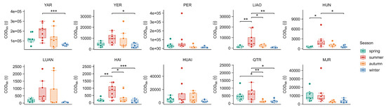
Figure 5.
Box plots and Tukey HSD test results of fluxes between different seasons. *: p-value < 0.05; **: p-value < 0.01; ***: p-value < 0.001.
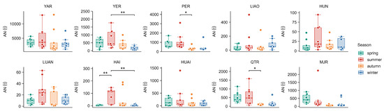
Figure 6.
Box plots and Tukey HSD test results of AN fluxes between different seasons. *: p-value < 0.05; **: p-value < 0.01.
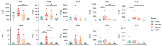
Figure 7.
Box plots and Tukey HSD test results of TP fluxes between different seasons. *: p-value < 0.05; **: p-value < 0.01; ***: p-value < 0.001.
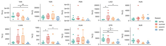
Figure 8.
Box plots and Tukey HSD test results of TN fluxes between different seasons. *: p-value < 0.05; **: p-value < 0.01.
For the AN flux, YER exhibited a significant difference between summer and winter (p-value < 0.01). PER showed a significant difference between summer and autumn (p-value < 0.05). HAI demonstrated significant differences both between spring and summer (p-value < 0.01) and between summer and winter (p-value < 0.01). QTR exhibited a significant difference between summer and autumn (p-value < 0.05). However, for YAR, LIAO, HUN, LUAN, HUAI, and MLR, no significant differences in AN flux were observed among the four seasons, which is consistent with the marginal seasonal significance of AN reported in Table 3 (F-statistic = 2.626, p-value = 0.051).
For TP flux, the difference patterns for YAR and YER are similar, with both showing significant differences between summer and winter; however, the TP flux difference between summer and winter is more pronounced for YAR (p-value < 0.001) than for YER (p-value < 0.05). The patterns for LIAO and HUN are also similar, as both exhibit significant differences between spring and summer (LIAO, p-value < 0.01; HUN, p-value < 0.05) and between summer and winter (LIAO, p-value < 0.05; HUN, p-value < 0.01). HAI displays significant differences in TP flux between spring and summer (p-value < 0.001), between summer and autumn (p-value < 0.05), and between summer and winter (p-value < 0.001). QTR shows significant differences between summer and autumn, as well as between summer and winter (p-value < 0.05). However, for PER, LUAN, MJR, and HUAI, no significant differences in TP flux were observed among the four seasons.
For TN flux, YAR shows significant differences to varying degrees between spring and winter (p-value < 0.05) and between summer and winter (p-value < 0.01). LIAO exhibits significant differences between spring and summer (p-value < 0.05), as well as between summer and winter (p-value < 0.05). HAI displays seasonal variations in TN flux similar to those of LIAO. QTR demonstrates significant differences between spring and autumn (p-value < 0.01), between spring and winter (p-value < 0.05), and between summer and autumn (p-value < 0.05). However, no seasonal differences in TN flux were observed for YER, PER, HUN, LUAN, HUAI, and MJR. Additionally, seasonal differences were detected in the fluxes of all four pollutants for the four rivers PER, LUAN, HUAI, and MLR.
3.3. Analysis of Variance for Flood Season and River Factors
Given the significant impact of seasonal fluctuations in river runoff on pollutant fluxes, it is essential to examine the correlation between river runoff and pollutant dynamics. However, because runoff data were already used in the calculation of pollutant fluxes in this study, conducting a correlation analysis between runoff and pollutant flux would be methodologically invalid. As an alternative, we analyzed the correlations between river runoff and pollutant concentrations. Figure 9 presents the seasonal correlation matrices between river runoff and the concentrations of four pollutants. The results show that the relationships between runoff and concentration are generally consistent across seasons. Moreover, a negative correlation is observed, suggesting that higher river runoff tends to dilute pollutant concentrations.
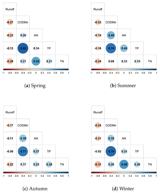
Figure 9.
The correlation matrix plot between river runoff and pollutant concentrations for different seasons.
Table 4 presents the results of a two-way ANOVA for the four pollutants across the factors of flood season and river.
Table 4.
Two-way ANOVA results on pollutant fluxes among flood season, non-flood season and rivers.
The results in Table 4 indicate that the effects of both flood season and river on pollutant fluxes are significantly different.
Regarding the foold seasonal effect, flood season and non-flood season has a highly significant difference on the fluxes of , AN, TP, and TN (p-value < 0.001); Regarding the river effect, the river factor shows significant difference on all pollutant fluxes (p-value < 0.001). Notably, the influence of the river factor is most significant for TP (F-statistic = 104.85), followed by TN (F-statistic = 60.264) and (F-statistic = 67.66); Regarding the interaction effect, the interaction between flood season and river significantly affects the fluxes of , TP, and TN (p-value < 0.001), but not AN (F-statistic = 1.088, p-value = 0.371), suggesting that the spatio-temporal variation of AN is primarily driven by the independent effects of flood season or river.
It should be noted that although the influence of rivers on pollutant fluxes is also discussed in Table 3, the results will be slightly different because we performed the two-way ANOVA.
Figure 10 presents the pairwise comparisons of the four pollutant fluxes among rivers, categorized by flood and non-flood seasons. During the flood season, YAR exhibits highly significant differences in the fluxes of , AN, TP, and TN compared to the other nine rivers (p-value < 0.001). PER shows significant differences in and TN fluxes relative to the other nine rivers; however, no significant difference in TP flux is observed between the PER and MLR, and its AN flux does not difference significantly from that of the eight rivers excluding YAR.
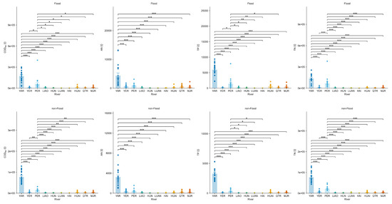
Figure 10.
Mean bar plots and Tukey HSD test results of pollutant fluxes between different rivers. *: p-value < 0.05; **: p-value < 0.01; ***: p-value < 0.001.
During the non-flood season, YAR exhibits significant differences (p-value < 0.001) in the fluxes of , AN, TP, and TN compared to the other nine rivers. PER shows significant differences in and TN fluxes relative to the other nine rivers. In addition, PER displays significant differences in AN flux when compared with YAR, LIAO, HUN, LUAN, and HAI. However, the AN flux of the Pearl River does not difference significantly from that of the eight rivers excluding YAR.
Figure 11 reports the comparative results of the four pollutant fluxes between the flood season and non-flood season across different rivers. Analysis of the results presented in Figure 11 reveals that:
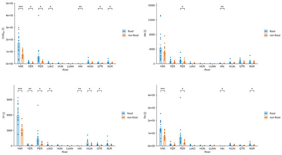
Figure 11.
Mean bar plots and T test results of pollutant fluxes between flood season and non-flood season. *: p-value < 0.05; **: p-value < 0.01; ***: p-value < 0.001.
For flux, significant differences between flood season and non-flood season are observed in seven rivers: YAR, YER, PER, LIAO, HAI, QTR, and MJR. For AN flux, only PER and HAI exhibit significant differences between the flood season and non-flood season, while no significant differences are observed in the other eight rivers. For TP flux, significant differences between the two periods are found in seven rivers: YAR, YER, PER, LIAO, HAI, HUAI, and QTR. For TN flux, significant differences between flood season and non-flood season occur in four rivers: YAR, PER, HAI, and MJR.
3.4. PCA Results
Table 5 and Table 6 presents the eigenvalue, variance percent, and cumulative variance percent of the PCA for different seasons and different flood seasons. Figure 12 presents the PCA results for ten rivers across different seasons. Figure 13 compares the PCA results of the ten rivers during flood and non-flood periods. The left panel of Figure 12 and Figure 13 reveals the spatial differentiation in the distribution of river pollutant fluxes between these periods, while the right panel quantifies the contribution weights of each pollutant flux to the principal components. A comprehensive analysis indicates the following:
Table 5.
PCA results between for different seasons.
Table 6.
PCA results between for flood season and non-flood season.
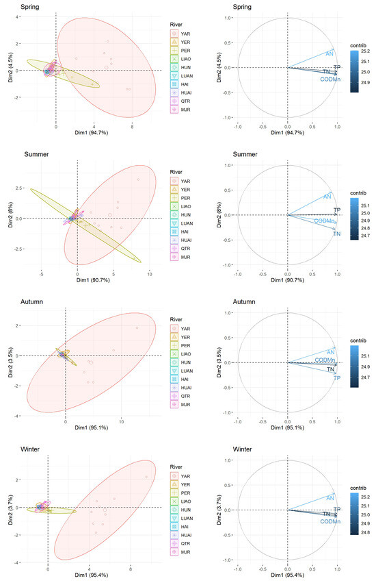
Figure 12.
PCA results between different seasons. Left: PCA profiles of ten rivers; Right: PCA loading of ten rivers.
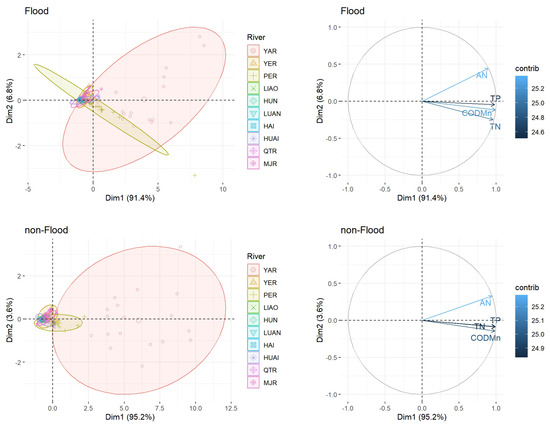
Figure 13.
PCA results between flood season and non-flood season. Left: PCA profiles of ten rivers; Right: PCA loading of ten rivers.
River samples from different seasons cluster separately in the principal component space, suggesting that seasonal changes significantly influence the overall distribution patterns of pollutants. For instance, summer and winter samples may be positioned at opposite ends of the principal component axis, reflecting the regulatory effects of seasonal factors such as water temperature and runoff on pollutant fluxes.The distribution profiles of the ten rivers exhibit spatial heterogeneity. YAR and PER are distinctly separated from others along the principal component axis, implying that their pollutant flux characteristics are unique.
It is worth noting that in all the principal component analyses presented above, the first principal component consistently have a high variance percent (>90%). This may be attributed to the fact that our study focuses on pollutant fluxes, which are calculated using river runoff. As a result, the different variables involved may share overlapping information, leading to redundancy and consequently inflating the variance percent captured by the first principal component.
4. Discussion
4.1. Spatial Heterogeneity of Pollutant Fluxes
Pollutant flux is an important indicator for assessing river ecological health and eutrophication [24]. Exploring the spatial variability of pollutant fluxes across different rivers offers essential insights to inform river management strategies [31]. This study reveals that there is significant spatial heterogeneity in the pollutant fluxes of rivers discharging into the sea in eastern China. This phenomenon is likely driven by the combined effects of watershed characteristics, the intensity of human activities, and hydrological conditions. This is consistent with previous studies on the relationship between human activities and environmental changes [1,32,33]. Two-way ANOVA (Table 3) indicates that the river factor have a highly significant influence on all pollutant fluxes (p-value < 0.001), with TP flux exhibiting the most pronounced spatial variability (F-statistic = 151.039), followed by TN and fluxes. This finding is consistent with the violin plot analysis in Figure 3, which shows that the pollutant fluxes in YAR are significantly higher than those in the other rivers—possibly due to YAR’s enormous runoff and its location in an economically developed region with intense human activities [34,35]. PER, which ranks second in terms of pollutant flux, may have its pollutant load closely linked to the dense industrial discharges and urban wastewater inputs from the Pearl River Delta [36,37].
Spatial differentiation is further corroborated by PCA results (Figure 12 and Figure 13). The PCA results confirm that YAR and PER are distinctly separated from the other rivers in the principal component space, with YAR, in particular, exhibiting a unique distribution pattern during both flood and non-flood periods (Figure 13). This differentiation may be attributed to the massive runoff of the Yangtze River basin [38], and agricultural pollution within the basin [39]. In contrast, northern rivers such as LIAO and LUAN display lower and more concentrated fluxes (Figure 3), likely due to the low runoff and seasonal flow interruptions [16,40].
Notably, HAI exhibited slightly higher pollutant fluxes than other northern rivers in 2021 (Figure 3), which may be associated with the high population density of the Beijing-Tianjin-Hebei urban agglomeration and the overloading of wastewater treatment facilities within its basin. Furthermore, interaction analysis indicates that the interaction effects between season and river (F-statistic = 0.493, p-value = 0.985) as well as between flood period and river (F-statistic = 1.088, p-value = 0.371) have no significant impact on AN flux, suggesting that AN flux is primarily controlled by either spatial or temporal factors independently, rather than by dynamic hydrological-climatic coupling mechanisms [18].
In summary, the spatial heterogeneity of pollutant fluxes is not only a product of natural geographical conditions but also reflects the pronounced regional imbalance of human activities. Future basin management should develop differentiated control strategies based on the specific pollutant source characteristics of each river. For instance, controlling non-point source pollution should be prioritized in the YAR and PER, whereas northern rivers require greater emphasis on improving water allocation and regulating industrial point-source discharges. These tailored strategies can further support existing policy frameworks by establishing river-specific reduction targets and monitoring protocols.
4.2. Mechanisms Underlying Seasonal Variations in Pollutant Fluxes
Investigating the variability of river pollutant fluxes across different seasons is of paramount importance, as it offers critical insights for understanding seasonal changes in pollutant fluxes and for guiding policy recommendations [41]. The data analysis in this study indicates that, except for AN flux, which exhibits only marginal significance, the fluxes of , TP, and TN display significant seasonal differences (Table 3, p-value < 0.001), underscoring the substantial impact of seasonal variation on pollutant fluxes. The underlying mechanisms behind this phenomenon can be primarily attributed to several factors.
First of all, seasonal variations in natural hydrological conditions are a important factor driving changes in river pollutant fluxes. In summer, increased rainfall and a significant rise in runoff not only speed up the transport of pollutants but may also flush or dilute them during short periods of high flow, leading to clear fluctuations in the measured pollutant fluxes [42]. For example, the significant differences in , TP, and TN fluxes between summer and winter for YAR and YER clearly reflect this hydrological effect (Figure 5, Figure 6, Figure 7 and Figure 8).
Secondly, temperature changes play a important role in the transformation and transport of pollutants. In summer, higher water temperatures can boost microbial activity, which accelerates the decomposition of organic matter and the transformation of nutrients, leading to changes in the concentrations of certain pollutants [43]. In contrast, the low temperatures of winter tend to slow down these biochemical reactions, resulting in more pronounced accumulation of pollutants [44]. These temperature-driven changes in reaction rates directly affect both the calculation of pollutant fluxes and their spatial-temporal distribution [45].
Furthermore, the seasonal patterns of human activities also play an vital role in the changes observed in pollutant fluxes [32]. In China, both agricultural production and industrial activities show clear seasonal trends [46,47]. For example, during summer, vigorous crop growth accompanied by frequent fertilization and irrigation leads to a significant increase in non-point source pollution from farmlands [48]. In winter, although agricultural activities decline, urban domestic sewage and industrial discharges tend to be more concentrated and steady, resulting in relatively higher pollutant fluxes. This effect is particularly noticeable for rivers such as YAR and PER, which are located in economically developed and densely populated areas, where seasonal fluctuations in human activities strongly influence pollutant flux regulation, which is consistent with previous researches [49,50].
Finally, examining the interaction effects, the interplay between seasonal variations and river-specific factors significantly influences the fluxes of , TP, and TN (Table 3, p-value < 0.001). However, this interaction does not have a notable effect on AN flux (Table 3, F-statistic = 0.493, p-value = 0.985). This suggests that the transport processes of certain pollutants, such as , TP, and TN, are predominantly governed by the coupling of hydrometeorological conditions and geographical characteristics [51]. In contrast, AN flux appears to be primarily controlled by specific factors, such as agricultural or urban discharges during particular periods [52].
In summary, the seasonal variations in pollutant fluxes result from the combined effects of natural hydrological conditions, temperature changes, and seasonal fluctuations in human activities. Future research should further explore the interaction mechanisms among these factors to provide more precise scientific evidence for regional water environment management and pollution prevention. In addition, our findings highlight the need to incorporate seasonal discharge of concentration dynamics into operational guidelines. For example, adjusting reservoir release schedules and agricultural fertilization windows to minimize peak pollutant loads.
4.3. Differences in Pollutant Fluxes Between Flood and Non-Flood Seasons
This study, by comparing pollutant fluxes during flood and non-flood seasons, revealed significant differences in pollutant fluxes under varying hydrological conditions. The results indicate that during the flood season, the dramatic increase in rainfall and runoff substantially alters hydrodynamic conditions, which in turn significantly affects the pollutant fluxes. For instance, the two-way ANOVA results in Table 4 show highly significant differences in the fluxes of , AN, TP, and TN between flood and non-flood seasons (p-value < 0.001), with TP flux being the most pronounced (F-statistic = 104.85). Moreover, the significant interaction effects between flood season and river for , TP, and TN (p-value < 0.001) further demonstrate that different rivers exhibit distinct pollutant fluxes characteristics during flood events. These differences may stem from the variations in rainfall intensity, runoff response, and pollutant sources among the basins [53,54].
Figure 10 and Figure 11, which display box plots and mean bar plots, clearly show that during the flood season, the pollutant flux in YAR is considerably higher than in the other nine rivers. This is likely due to the strong runoff generated by widespread rainfall and concentrated anthropogenic pressures within the Yangtze basin [55]. In contrast, during the non-flood season, although YAR still exhibits significant differences compared with other rivers (p-value < 0.001), the overall flux levels are lower. This reflects that under weaker runoff conditions in the non-flood season, the capacity for pollutant transport and diffusion is limited [56].
Furthermore, the study found that PER shows significant differences in and TN fluxes between flood and non-flood seasons, whereas its TP flux did not display significant changes in some cases. This phenomenon might be related to the dense industrial and urban discharges in the Pearl River Delta region, where high flows during the flood season may dilute certain pollutants, while in the non-flood season, pollutant accumulation is more pronounced [57,58].
Overall, the substantial impact of heavy rainfall and increased runoff during flood events on pollutant fluxes can be attributed to two primary factors. First, the high flow during the flood season accelerates the transport of pollutants, potentially triggering short-term surges or dilution effects [59]. Second, differences in geography, climate, and the distribution of human activities among river basins lead to distinct pollutant release and dispersion patterns during flood events [60]. The results of this study will provide more precise scientific evidence for the development of effective regional water environment management and pollution prevention strategies. These findings underscore the importance of dynamic flood season management to mitigate peak pollutant loads.
5. Conclusions
Through detailed analysis, this study explores pollutant fluxes in ten major rivers discharging into the sea in eastern China, revealing significant spatiotemporal differences. The findings indicate that, under the influence of hydrological conditions, climate change, and anthropogenic intervention, pollutant loads in YAR and PER are markedly higher than in other rivers. Furthermore, seasonal variations and flood events have a substantial impact on pollutant fluxes. Statistical analyses demonstrate that the spatiotemporal distribution of pollutant fluxes reflects not only the diversity of natural conditions but also the imbalance in regional economic activities. Based on these results, the study provides scientific support for regional water management and pollution control. It is recommended that future river management strategies be tailored to the unique characteristics of each basin and that further investigation into the coupled effects of multiple factors be conducted to ensure sustainable water utilization and the protection of ecological security.
Despite these insights, this study has several limitations. First, our analysis does not include detailed data on point-source discharges, which may underestimate the contribution of industrial and municipal effluents. Second, monitoring coverage and sampling vary among the rivers, potentially biasing comparisons. Finally, the reliance on annual and seasonal aggregates may mask shorter-term episodic events. Future work should address these gaps by integrating high-resolution discharge and effluent data alongside more uniform monitoring networks.
Author Contributions
Conceptualization, W.G. and Y.Z.; methodology, L.W.; software, L.W. and S.L.; validation, L.W., S.M. and Y.C.; formal analysis, L.W. and S.L.; investigation, L.W.; resources, L.W.; data curation, L.W.; writing—original draft preparation, L.W.; writing—review and editing, S.M. and S.L.; visualization, L.W. and S.L.; supervision, Y.Z.; project administration, W.G.; funding acquisition, S.M. All authors have read and agreed to the published version of the manuscript.
Funding
This research was funded by Research Project on Ecological Protection and High-Quality Development in the Yellow River Basin, China No. (2022-YRUC-01-0602).
Institutional Review Board Statement
Not applicable.
Informed Consent Statement
Not applicable.
Data Availability Statement
The water quality data for this study were sourced from China National Environmental Monitoring Centre (available at https://www.cnemc.cn, accessed on 16 February 2024). The hydrological data were obtained from China River Sediment Bulletin, which is published by Ministry of Water Resources of the People’s Republic of China (available at http://www.mwr.gov.cn, accessed on 2 November 2024).
Conflicts of Interest
The authors declare no conflicts of interest.
Abbreviations
The following abbreviations are used in this manuscript:
| Yangtze River | YAR |
| Yellow River | YER |
| Pearl River | PER |
| Liaohe River | LIAO |
| Hunhe River | HUN |
| Luanhe River | LUAN |
| Haihe River | HAI |
| Huaihe River | HUAI |
| Qiantang River | QTR |
| Minjiang River | MJR |
| Permanganate Index | |
| Ammonia Nitrogen | AN |
| Total Phosphorus | TP |
| Total Nitrogen | TN |
References
- Cheng, X.; Chen, L.; Sun, R.; Kong, P. Land use changes and socio-economic development strongly deteriorate river ecosystem health in one of the largest basins in China. Sci. Total Environ. 2018, 616, 376–385. [Google Scholar] [CrossRef] [PubMed]
- Zhang, Y.; Sun, M.; Yang, R.; Li, X.; Zhang, L.; Li, M. Decoupling water environment pressures from economic growth in the Yangtze River Economic Belt, China. Ecol. Indic. 2021, 122, 107314. [Google Scholar] [CrossRef]
- Fan, H.; Huang, H. Response of coastal marine eco-environment to river fluxes into the sea: A case study of the Huanghe (Yellow) River mouth and adjacent waters. Mar. Environ. Res. 2008, 65, 378–387. [Google Scholar] [CrossRef]
- Han, Q.; Huang, X.; Xing, Q.; Shi, P. A review of environment problems in the coastal sea of South China. Aquat. Ecosyst. Health Manag. 2012, 15, 108–117. [Google Scholar] [CrossRef]
- Akhtar, N.; Syakir Ishak, M.I.; Bhawani, S.A.; Umar, K. Various natural and anthropogenic factors responsible for water quality degradation: A review. Water 2021, 13, 2660. [Google Scholar] [CrossRef]
- Swaney, D.P.; Hong, B.; Ti, C.; Howarth, R.W.; Humborg, C. Net anthropogenic nitrogen inputs to watersheds and riverine N export to coastal waters: A brief overview. Curr. Opin. Environ. Sustain. 2012, 4, 203–211. [Google Scholar] [CrossRef]
- Frigstad, H.; Kaste, Ø.; Deininger, A.; Kvalsund, K.; Christensen, G.; Bellerby, R.G.; Sørensen, K.; Norli, M.; King, A.L. Influence of riverine input on Norwegian coastal systems. Front. Mar. Sci. 2020, 7, 332. [Google Scholar] [CrossRef]
- Mishra, R.K. Fresh water availability and its global challenge. Br. J. Multidiscip. Adv. Stud. 2023, 4, 1–78. [Google Scholar] [CrossRef]
- Song, X.; Ravesteijn, W.; Frostell, B.; Wennersten, R. Managing water resources for sustainable development: The case of integrated river basin management in China. Water Sci. Technol. 2010, 61, 499–506. [Google Scholar] [CrossRef]
- Li, P.; Wang, D.; Li, W.; Liu, L. Sustainable water resources development and management in large river basins: An introduction. Environ. Earth Sci. 2022, 81, 179. [Google Scholar] [CrossRef]
- Koch, S.; Kahle, P.; Lennartz, B. Spatio-temporal analysis of phosphorus concentrations in a North-Eastern German lowland watershed. J. Hydrol. Reg. Stud. 2018, 15, 203–216. [Google Scholar] [CrossRef]
- Mamun, M.; Jargal, N.; An, K.G. Spatio-temporal characterization of nutrient and organic pollution along with nutrient-chlorophyll-a dynamics in the Geum River. J. King Saud Univ.-Sci. 2022, 34, 102270. [Google Scholar] [CrossRef]
- Bu, H.; Tan, X.; Li, S.; Zhang, Q. Temporal and spatial variations of water quality in the Jinshui River of the South Qinling Mts., China. Ecotoxicol. Environ. Saf. 2010, 73, 907–913. [Google Scholar] [CrossRef] [PubMed]
- Turner, R.E.; Rabalais, N.N.; Justic’, D.; Dortch, Q. Global patterns of dissolved N, P and Si in large rivers. Biogeochemistry 2003, 64, 297–317. [Google Scholar] [CrossRef]
- Varol, M. Temporal and spatial dynamics of nitrogen and phosphorus in surface water and sediments of a transboundary river located in the semi-arid region of Turkey. CATENA 2013, 100, 1–9. [Google Scholar] [CrossRef]
- Wang, H.; Sun, L.; Liu, Z.; Luo, Q. Spatial distribution and seasonal variations of heavy metal contamination in surface waters of Liaohe River, Northeast China. Chin. Geogr. Sci. 2017, 27, 52–62. [Google Scholar] [CrossRef]
- Rattan, K.; Corriveau, J.; Brua, R.; Culp, J.; Yates, A.; Chambers, P. Quantifying seasonal variation in total phosphorus and nitrogen from prairie streams in the Red River Basin, Manitoba Canada. Sci. Total Environ. 2017, 575, 649–659. [Google Scholar] [CrossRef]
- Li, X.; Xu, W.; Song, S.; Sun, J. Sources and spatiotemporal distribution characteristics of nitrogen and phosphorus loads in the Haihe River Basin, China. Mar. Pollut. Bull. 2023, 189, 114756. [Google Scholar] [CrossRef]
- Chang, F.J.; Chen, P.A.; Chang, L.C.; Tsai, Y.H. Estimating spatio-temporal dynamics of stream total phosphate concentration by soft computing techniques. Sci. Total Environ. 2016, 562, 228–236. [Google Scholar] [CrossRef]
- Wang, L.; Han, X.; Zhang, Y.; Zhang, Q.; Wan, X.; Liang, T.; Song, H.; Bolan, N.; Shaheen, S.M.; White, J.R.; et al. Impacts of land uses on spatio-temporal variations of seasonal water quality in a regulated river basin, Huai River, China. Sci. Total Environ. 2023, 857, 159584. [Google Scholar] [CrossRef]
- Dou, M.; Zhang, Y.; Li, G. Temporal and spatial characteristics of the water pollutant concentration in Huaihe River Basin from 2003 to 2012, China. Environ. Monit. Assess. 2016, 188, 1–18. [Google Scholar] [CrossRef]
- Floehr, T.; Xiao, H.; Scholz-Starke, B.; Wu, L.; Hou, J.; Yin, D.; Zhang, X.; Ji, R.; Yuan, X.; Ottermanns, R.; et al. Solution by dilution?—A review on the pollution status of the Yangtze River. Environ. Sci. Pollut. Res. 2013, 20, 6934–6971. [Google Scholar] [CrossRef] [PubMed]
- Jin, Z.; Chen, L.; Li, F.; Pan, Z.; Jin, M. Effects of water transfer on water quality and estimation of the pollutant fluxes from different sources into West Lake, Hangzhou City, China. Environ. Earth Sci. 2015, 73, 1091–1101. [Google Scholar] [CrossRef]
- Wu, G.; Cao, W.; Wang, F.; Su, X.; Yan, Y.; Guan, Q. Riverine nutrient fluxes and environmental effects on China’s estuaries. Sci. Total Environ. 2019, 661, 130–137. [Google Scholar] [CrossRef] [PubMed]
- Zeileis, A.; Grothendieck, G. zoo: S3 infrastructure for regular and irregular time series. J. Stat. Softw. 2005, 14, 1–27. [Google Scholar] [CrossRef]
- Grosjean, P.; Ibanez, F.; Etienne, M. Pastecs: Package for Analysis of Space-Time Ecological Series, R package version; 2018; Volume 1, p. 21. Available online: https://github.com/SciViews/pastecs (accessed on 30 April 2025).
- Engler, J.B. Tidyplots empowers life scientists with easy code-based data visualization. bioRxiv 2024. [Google Scholar] [CrossRef]
- Wickham, H. ggplot2: Elegant Graphics for Data Analysis; Springer: New York, NY, USA, 2016. [Google Scholar]
- Lê, S.; Josse, J.; Husson, F. FactoMineR: An R package for multivariate analysis. J. Stat. Softw. 2008, 25, 1–18. [Google Scholar] [CrossRef]
- Kassambara, A.; Mundt, F. factoextra: Extract and Visualize the Results of Multivariate Data Analyses, R package version 1.0.7.999; 2020; Available online: https://cran.r-project.org/web/packages/factoextra/readme/README.html (accessed on 30 April 2025).
- Wu, L.; Liu, K.; Wang, Z.; Yang, Y.; Sang, R.; Zhu, H.; Wang, X.; Pang, Y.; Tong, J.; Liu, X.; et al. Temporal–Spatial Variations in Physicochemical Factors and Assessing Water Quality Condition in River–Lake System of Chaohu Lake Basin, China. Sustainability 2025, 17, 2182. [Google Scholar] [CrossRef]
- Cui, M.; Guo, Q.; Wei, R.; Tian, L. Human-driven spatiotemporal distribution of phosphorus flux in the environment of a mega river basin. Sci. Total Environ. 2021, 752, 141781. [Google Scholar] [CrossRef]
- Lämmle, L.; Perez Filho, A.; Donadio, C.; Arienzo, M.; Ferrara, L.; Santos, C.d.J.; Souza, A.O. Anthropogenic pressure on hydrographic basin and coastal erosion in the delta of Paraíba do Sul River, southeast Brazil. J. Mar. Sci. Eng. 2022, 10, 1585. [Google Scholar] [CrossRef]
- Xu, H.; Chen, Z.; Finlayson, B.; Webber, M.; Wu, X.; Li, M.; Chen, J.; Wei, T.; Barnett, J.; Wang, M. Assessing dissolved inorganic nitrogen flux in the Yangtze River, China: Sources and scenarios. Glob. Planet. Change 2013, 106, 84–89. [Google Scholar] [CrossRef]
- Lou, B.; Zhuo, H.; Zhou, Z.; Wu, Y.; Wang, R. Analysis on alteration of water quality and pollutant fluxes in the Yangtze mainstem during recently 18 years. Res. Environ. Sci. 2020, 33, 1150–1162. [Google Scholar] [CrossRef]
- Zhang, K.; Zhang, B.Z.; Li, S.M.; Zeng, E.Y. Regional dynamics of persistent organic pollutants (POPs) in the Pearl River Delta, China: Implications and perspectives. Environ. Pollut. 2011, 159, 2301–2309. [Google Scholar] [CrossRef]
- Zhang, S.; Zhang, H. Anthropogenic impact on long-term riverine CODMn, BOD, and nutrient flux variation in the Pearl River Delta. Sci. Total Environ. 2023, 859, 160197. [Google Scholar] [CrossRef]
- Chen, J.; Wu, X.; Finlayson, B.L.; Webber, M.; Wei, T.; Li, M.; Chen, Z. Variability and trend in the hydrology of the Yangtze River, China: Annual precipitation and runoff. J. Hydrol. 2014, 513, 403–412. [Google Scholar] [CrossRef]
- Wang, H.; Liu, C.; Xiong, L.; Wang, F. The spatial spillover effect and impact paths of agricultural industry agglomeration on agricultural non-point source pollution: A case study in Yangtze River Delta, China. J. Clean. Prod. 2023, 401, 136600. [Google Scholar] [CrossRef]
- Li, D.; Zhang, B.; Li, H.; Wu, E.; Zhao, J.; Chen, Q.; Bai, X.; Li, Y.F.; Li, B.; Wu, G.; et al. Heavy metals pollution and the associated ecological risks along the Luanhe River basin in North China. J. Environ. Manag. 2025, 376, 124452. [Google Scholar] [CrossRef]
- Huang, C.W.; Li, Y.L.; Lin, C.; Bui, X.T.; Vo, T.D.H.; Ngo, H.H. Seasonal influence on pollution index and risk of multiple compositions of microplastics in an urban river. Sci. Total Environ. 2023, 859, 160021. [Google Scholar] [CrossRef] [PubMed]
- Alifujiang, Y.; Abuduwaili, J.; Ge, Y. Trend analysis of annual and seasonal river runoff by using innovative trend analysis with significant test. Water 2021, 13, 95. [Google Scholar] [CrossRef]
- Tang, G.; Zheng, X.; Hu, S.; Li, B.; Chen, S.; Liu, T.; Zhang, B.; Liu, C. Microbial metabolism changes molecular compositions of riverine dissolved organic matter as regulated by temperature. Environ. Pollut. 2022, 306, 119416. [Google Scholar] [CrossRef]
- Van Vliet, M.T.; Thorslund, J.; Strokal, M.; Hofstra, N.; Flörke, M.; Ehalt Macedo, H.; Nkwasa, A.; Tang, T.; Kaushal, S.S.; Kumar, R.; et al. Global river water quality under climate change and hydroclimatic extremes. Nat. Rev. Earth Environ. 2023, 4, 687–702. [Google Scholar] [CrossRef]
- Wang, J.H.; Li, C.; Xu, Y.P.; Li, S.Y.; Du, J.S.; Han, Y.P.; Hu, H.Y. Identifying major contributors to algal blooms in Lake Dianchi by analyzing river-lake water quality correlations in the watershed. J. Clean. Prod. 2021, 315, 128144. [Google Scholar] [CrossRef]
- Huang, X.; Song, Y.; Li, M.; Li, J.; Zhu, T. Harvest season, high polluted season in East China. Environ. Res. Lett. 2012, 7, 044033. [Google Scholar] [CrossRef]
- Wang, Y.; Xin, J.; Li, Z.; Wang, S.; Wang, P.; Hao, W.M.; Nordgren, B.L.; Chen, H.; Wang, L.; Sun, Y. Seasonal variations in aerosol optical properties over China. J. Geophys. Res. Atmos. 2011, 116. [Google Scholar] [CrossRef]
- Savci, S. An agricultural pollutant: Chemical fertilizer. Int. J. Environ. Sci. Dev. 2012, 3, 73. [Google Scholar] [CrossRef]
- Ali, S.H.; Puppim de Oliveira, J.A. Pollution and economic development: An empirical research review. Environ. Res. Lett. 2018, 13, 123003. [Google Scholar] [CrossRef]
- Muyibi, S.A.; Ambali, A.R.; Eissa, G.S. The impact of economic development on water pollution: Trends and policy actions in Malaysia. Water Resour. Manag. 2008, 22, 485–508. [Google Scholar] [CrossRef]
- Pizarro, H.; Rodríguez, P.; Bonaventura, S.M.; O’Farrell, I.; Izaguirre, I. The sudestadas: A hydro-meteorological phenomenon that affects river pollution (River Luján, South America). Hydrol. Sci. J. 2007, 52, 702–712. [Google Scholar] [CrossRef]
- Zhang, W.; Swaney, D.P.; Hong, B.; Howarth, R.W.; Li, X. Influence of rapid rural-urban population migration on riverine nitrogen pollution: Perspective from ammonia-nitrogen. Environ. Sci. Pollut. Res. 2017, 24, 27201–27214. [Google Scholar] [CrossRef]
- Li, Z.; Tian, C.; Sheng, Y. Fluxes of chemical oxygen demand and nutrients in coastal rivers and their influence on water quality evolution in the Bohai Sea. Reg. Stud. Mar. Sci. 2022, 52, 102322. [Google Scholar] [CrossRef]
- Wang, X.; Ding, L.; Wu, Y.; Bol, R. Combined effects of flood, drought and land use dominate water quality and nutrient exports in Jialing River basin, SW China. Sci. Total Environ. 2024, 954, 176733. [Google Scholar] [CrossRef] [PubMed]
- Cui, L.; Wang, L.; Lai, Z.; Tian, Q.; Liu, W.; Li, J. Innovative trend analysis of annual and seasonal air temperature and rainfall in the Yangtze River Basin, China during 1960–2015. J. Atmos. Sol.-Terr. Phys. 2017, 164, 48–59. [Google Scholar] [CrossRef]
- Jiang, P.; Dong, B.; Huang, G.; Tong, S.; Zhang, M.; Li, S.; Zhang, Q.; Xu, G. Study on the sediment and phosphorus flux processes under the effects of mega dams upstream of Yangtze River. Sci. Total Environ. 2023, 860, 160453. [Google Scholar] [CrossRef]
- Zhou, N.; Westrich, B.; Jiang, S.; Wang, Y. A coupling simulation based on a hydrodynamics and water quality model of the Pearl River Delta, China. J. Hydrol. 2011, 396, 267–276. [Google Scholar] [CrossRef]
- Zhao, Y.; Song, Y.; Cui, J.; Gan, S.; Yang, X.; Wu, R.; Guo, P. Assessment of water quality evolution in the Pearl River Estuary (South Guangzhou) from 2008 to 2017. Water 2019, 12, 59. [Google Scholar] [CrossRef]
- Tan, L.; Wang, Z.; Bai, Y.; Huang, X. Short-term responses of nutrients and algal biomass in a eutrophic shallow lake to different scales of water transfer. Sci. Total Environ. 2023, 880, 163321. [Google Scholar] [CrossRef]
- Bhuiyan, A.B.; Mokhtar, M.B.; Toriman, M.E.; Gasim, M.B.; Ta, G.C.; Elfithri, R.; Razman, M.R. The environmental risk and water pollution: A review from the river basins around the world. Am.-Eurasian J. Sustain. Agric. 2013, 7, 126–136. [Google Scholar]
Disclaimer/Publisher’s Note: The statements, opinions and data contained in all publications are solely those of the individual author(s) and contributor(s) and not of MDPI and/or the editor(s). MDPI and/or the editor(s) disclaim responsibility for any injury to people or property resulting from any ideas, methods, instructions or products referred to in the content. |
© 2025 by the authors. Licensee MDPI, Basel, Switzerland. This article is an open access article distributed under the terms and conditions of the Creative Commons Attribution (CC BY) license (https://creativecommons.org/licenses/by/4.0/).