Do Regional Differences Matter? Spatiotemporal Evolution and Convergence of Household Carbon Emissions in China

Abstract

Understanding how household carbon emissions vary across time and regions is essential for promoting low-carbon lifestyles and advancing sustainability, yet this dimension remains underexplored—especially in large, diverse economies like China. This study addresses that gap by analyzing household carbon emissions across 29 Chinese provinces from 2000 to 2022, focusing on regional differences and convergence patterns. Using spatial and convergence models, we find persistent clustering—where provinces with high or low emissions group together—though these patterns shift gradually. Emissions have generally risen nationwide, with convergence trends emerging in the east, central, south, and north, while the west and northeast show inconsistent dynamics. Notably, emissions in one province are influenced by those in neighboring provinces, particularly in central China, due to close economic and energy ties. Industrial structure slows convergence at the national level, whereas stronger economic development, better education, and higher industrialization contribute to narrowing regional disparities—especially in southern China. These findings offer new insights for designing region-specific strategies that align household emissions management with China’s broader climate and sustainability goals.

1. Introduction

Carbon emissions have garnered significant global attention amid the backdrop of escalating global climate change. The acceleration of industrialization and urbanization worldwide has led to a steep surge in energy consumption, resulting in a continuous augmentation of greenhouse gas emissions. According to the Emissions Gap Report 2020 published by the United Nations Environment Programme, household consumption emissions account for two-thirds of global carbon emissions [1]. China, one of the largest carbon-emitting countries, exhibits household consumption carbon emissions that attract extensive academic and policy attention. China’s household carbon emissions are rising rapidly, fueled by economic growth and higher living standards. Household consumption constitutes approximately 26% of China’s total energy consumption and 30% of its carbon emissions [2]. Consequently, conducting in-depth research on the evolving characteristics of carbon emissions from Chinese residents’ consumption and fostering a transition towards low-carbon and green consumption patterns represent crucial avenues for achieving sustainable economic and social development.

From the initial identification of, the quantitative assessment of, and mitigation strategies for carbon emissions to the contemporary evaluation of policy impacts, extensive research has been conducted. Gao et al. constructed a non-competitive input–output model to measure the embodied carbon emissions of 28 industrial sectors in China spanning 2005 to 2017 [3]. The findings revealed that China’s embodied and direct carbon emissions exhibited an overall upward trend, with notable differences in the total volume, growth rate, and rate of change. Feng et al. found that implementing carbon emission policies can significantly promote carbon emission reduction, and technological capacity is the main channel for carbon emission policies to encourage carbon emission reduction [4].

Scholars have increasingly focused on the convergence characteristics of carbon emissions, aiming to elucidate the dynamic fluctuations in carbon emission levels across different regions. Borozan employed the logarithmic regression method to study institutional convergence within the European Union and discovered that the influence of institutional quality on carbon dioxide emissions varies among distinct convergence clubs [5]. Shi and Huang demonstrated that the energy-related carbon emission efficiencies across the Yangtze River Economic Belt and its midstream and upstream segments exhibited σ-convergence traits [6]. In contrast, the downstream segment did not display such convergence. Notably, absolute β and conditional β convergence were observed in the upstream, midstream, and downstream regions, each exhibiting distinct spatial effects. Ren et al. investigated the role of climate vulnerability in global carbon emissions based on a panel dataset encompassing 101 countries from 2012 to 2019 [7]. Their study revealed a distinct spatial convergence pattern in global carbon emissions, with climate vulnerability facilitating this spatial convergence. Akram et al. examined the convergence patterns of carbon emissions in India and proposed a phased approach to reducing per capita carbon dioxide emissions by targeting specific state groups [8].

As residents’ consumption levels have risen, carbon emissions stemming from household consumption have garnered increasing attention. Basso et al. emphasized the necessity of understanding potential distributional impacts when assessing the importance of emission reduction policies [9]. To evaluate this heterogeneity, they quantified and analyzed the consumption emission intensity of Spanish households. Notably, except for the poorest households, emission intensity decreased with increasing income, peaking among households headed by middle-aged individuals (40 years old). Lian et al. analyzed the spatiotemporal evolution characteristics of provincial household carbon consumption emissions (HCCEs) in China using the Theil index and spatial autocorrelation [10]. Their findings revealed an average annual growth rate of 11.90% for HCCEs. Additionally, they observed a spatial agglomeration effect on per capita HCCE. Using input–output tables, Pang et al. calculated indirect carbon emissions from household consumption of middle-income groups in urban and rural areas from 2012 to 2018 [11]. The results indicated an increasing trend in indirect carbon emission intensity per household consumption (ICEHC) among middle-income groups in the Yangtze River Economic Belt, with notable spatial disparities, higher in the eastern region and lower in the western region. Su et al. proposed a dynamic household energy consumption and carbon emission assessment model from a residential perspective [12]. This model evaluated the average carbon emissions of households under three dynamic scenarios spanning from 2020 to 2060, revealing an overall downward trend. Cao et al. calculated the carbon emissions of the entire production end, including capital formation, resulting from Chinese household consumption using optimized data on the relationship between household consumption and production industries [13]. Their findings showed a steady increase in carbon emissions from Chinese household consumption between 2005 and 2015, with nearly 50% attributed to the rapid growth of household consumption. Some scholars have also conducted research from a micro-level perspective. Chen et al. analyzed the factors influencing direct household carbon emissions (DHCEs) and indirect household carbon emissions (IHCEs) in urban and rural areas of Fujian Province from 2006 to 2018 [14]. Their results indicated that per capita consumption expenditure positively impacted both DHCEs and IHCEs in urban and rural areas. Jiang et al. evaluated the spatial heterogeneity of household energy consumption and carbon emissions at the community scale in Guangzhou using a community-scale household energy consumption survey database [15]. They employed exploratory spatial data analysis and the standard deviation ellipse method and found significant spatial heterogeneity in household energy consumption carbon emissions. Wang and Yang utilized urban and rural statistical data spanning from 1999 to 2010 in China to compute the energy ecological footprint (EEF) associated with indirect energy consumption [16]. Their findings revealed that, for urban dwellers, the EEF of indirect energy use exhibited an upward trajectory. Liu et al. studied the impact of household consumption on carbon emissions using provincial data from China spanning from 1995 to 2017 [17]. They found that household consumption increases carbon emissions.

The academic community extensively researched the factors influencing carbon emissions stemming from household consumption. In terms of research methodologies, the ordinary least-squares method, the STIRPAT model, and the input–output method have all been employed. Lian et al. analyzed urban–rural disparities, spatiotemporal patterns, and agglomeration characteristics associated with household carbon emissions [18]. The results reveal that educational attainment has a suppressive effect on rural HCCEs. Peng et al. further observed that per capita income/consumption was the primary contributor to the increase in household emissions over most periods, while population changes also demonstrated a weak positive impact [19]. Conversely, the intermediate input–output structure and carbon emission intensity were the primary offsetting factors for household emissions. Wang et al. argued that community type has a significant bearing on the characteristics of household carbon emissions and their driving factors [20].

This paper focuses on 29 provinces in China, adopting a regional disparity perspective. The level of consumer carbon emissions is measured, the Theil index is employed to analyze regional disparities in household carbon emissions across China, and Moran’s index is used to analyze the spatial agglomeration characteristics of these emissions. Furthermore, the paper employs the kernel density analysis method to explore the spatiotemporal evolution of consumer carbon emissions. On this foundation, it investigates the convergence characteristics of consumer carbon emission levels in China using spatial exploration and convergence analysis techniques. This paper is important for advancing low-carbon consumption practices and achieving green economic transformation and sustainable development.

The potential contributions of this paper are the following. First, while most existing studies have analyzed the heterogeneity in consumption-based carbon emission levels among different provinces using the four major regional classifications of east, central, west, and northeast China, the scant literature is grounded in the north–south differentiation perspective, and studies that integrate the four major regions with north–south differences are exceedingly rare. This paper innovatively combines China’s north–south geographical differences with the traditional four-region framework. Taking “Do regional differences matter?” as a novel entry point, we facilitate a deeper exploration of the disparities in characteristics of residential consumption-based carbon emission changes and their convergence patterns across diverse regions. This approach provides new analytical lenses for comprehending interregional disparities in residential carbon emission levels. Second, existing studies frequently concentrate on time series analysis or static comparisons within a single region. In contrast, this study organically integrates the Theil index, Moran’s index, Kernel Density Estimation (KDE), and spatial convergence analysis. This approach addresses the limitation of conventional panel models that neglect spatial dependence and enables a multidimensional systematic examination spanning static distribution to dynamic evolution and global patterns to local characteristics. By incorporating spatial weight matrices into traditional convergence tests, we innovatively resolve the identification challenge of carbon emission convergence mechanisms under regional interaction effects. Finally, this study analyzes trends and cyclical patterns in consumption-based carbon emission levels across diverse spatial and temporal scales, both nationally and regionally. By capturing the micro-level impacts of regional disparities—such as climate conditions, economic models, and consumption habits—on residential carbon emissions, this research enhances understanding of the dynamics and complexity underlying consumption-driven emission patterns. These insights provide a differentiated empirical foundation for designing regionally coordinated emission reduction policies. Furthermore, innovatively tailored to China’s pronounced interregional disparities in economic development levels and consumption behaviors, this study proposes a suite of region-specific carbon mitigation strategies that account for local economic and geographical characteristics. This framework offers actionable guidance for policymakers to craft scientifically informed, context-sensitive emission reduction plans. Beyond China, the study establishes a replicable empirical paradigm for exploring consumption-side carbon reduction pathways globally, contributing not only to advancing low-carbon regional development in China but also offering valuable lessons for shaping equitable and effective carbon mitigation policies worldwide.

2. Methodology

This study establishes a five-stage cascading analytical framework of “household consumption carbon emission accounting → analysis of regional disparities → spatial autocorrelation analysis → dynamic evolution → convergence analysis”. First, we quantify residential consumption-based carbon emissions across China’s provincial-level regions using the carbon emission coefficient method. Subsequently, the Theil index examines regional disparities in household consumption carbon emission levels among different areas. Second, Moran’s I index is applied to identify spatial autocorrelation characteristics in these emissions. Following this, Kernel Density Estimation (KDE) delineates dynamic evolutionary patterns of consumption-related carbon emissions among China’s regional clusters. Finally, σ and β convergence models are constructed to investigate emission convergence mechanisms systematically.

2.1. Measurement of Carbon Emission Levels from Household Consumption

Direct carbon emissions pertain to the emissions generated by residents’ direct energy consumption in their daily lives [21]. Utilizing the carbon emission coefficient methodology published by the Intergovernmental Panel on Climate Change (IPCC), the direct emission inventory approach is employed to quantify direct carbon emissions from household consumptions [22]. The precise formula is outlined as follows:

$$C_d={\displaystyle \sum D{E}_i\times D{F}_i}$$

(1)

$$D{E}_i=F_i{C}_i$$

(2)

$$D{F}_i=NC{V}_i\times CE{F}_i\times CO{F}_i\times {\displaystyle \frac{44}{12}}$$

(3)

where C_d denotes the total direct carbon emissions from household consumption, and DE_i signifies the emission level associated with the i-th energy source. At the same time, F_i represents the standard coal conversion coefficient for the i-th energy source. C_i denotes the original consumption of this energy source. DF_i is the emission factor of the i-th energy source, and NCV_i indicates its net calorific value. CEF_i represents the carbon emission coefficient, and COF_i signifies the carbon oxidation factor. The numerals 44 and 12 correspond to the molecular weights of carbon dioxide and carbon, respectively.

Indirect carbon emissions are generated by the production and processing of various goods and services consumed by residents [23,24]. Drawing upon research findings from the China Family Panel Studies (CFPS), this study classifies indirect carbon emissions generated by household consumption into eight distinct categories, as outlined in

Table 1. Indicators for household consumption carbon emission level.

Carbon Emission Categories	Major Categories	Subcategories
Direct carbon emissions	Coals	Raw coal	Refined coal	Coke (processed coal used in blast furnace)
	Petroleum	Petroleum
	Diesel	Gasoline	Kerosene	Fuel oil	Diesel oil
	Crude oil
	Liquefied petroleum gas	Liquefied petroleum gas
	Gas (fuel)	Coke oven gas	Blast furnace gas	Converter gas	Other gases
	Thermodynamic	Thermal energy
	Electrical power	Electrical power
Indirect carbon emissions	Food, tobacco, and alcohol
	Clothing
	Living
	Daily necessities and services
	Medical care
	Transportation and communication
	Education, culture, and entertainment
	Other

. Adopting the methodology of Wei et al. [25], the consumer lifestyle approach is utilized. The specific formula employed is the following:

$$C_{in}={\displaystyle {\sum }_{i=1}^8{Q}_{i}P{L}_i}$$

(4)

where C_in represents the indirect carbon emissions from household consumption, Q_i denotes per capita consumption expenditure on consumer goods, P represents the total population, and L_i represents the carbon emission coefficients of the eight major categories of consumption expenditures [26].

The total household consumption carbon emissions (HCCEs) are calculated by aggregating direct and indirect carbon emissions [27]. Specifically, this is accomplished as follows:

$$Hcce=C_d+C_{in}$$

(5)

2.2. Theil Index

The Theil index is employed to measure regional inequality. This index decomposes the overall disparity into intra-group and inter-group components, enabling the identification of both the magnitude and sources of variation. Consequently, it has been widely utilized in regional disparity research. The mathematical formulation is expressed as follows:

$$T={\displaystyle \frac{1}{n}}{\displaystyle \sum _i^n\frac{Z_i}{u}\times \ln \frac{Z_i}{u}}$$

(6)

$$T=T_w+T_b$$

(7)

$$T_w={\displaystyle \sum _{k=1}^m\frac{n_k}{n}}\times {\displaystyle \frac{u_k}{u}}\times T_k$$

(8)

$$T_b={\displaystyle \sum _{k=1}^m\frac{n_k}{n}}\times {\displaystyle \frac{u_k}{u}}\times \ln {\displaystyle \frac{u_k}{u}}$$

(9)

T denotes the overall Theil index; n represents the number of provinces; Z_i indicates the level of carbon emissions from the residential consumption of the i-th province after sorting provinces in ascending order of carbon emissions; u signifies the mean value of residential consumption carbon emissions across all provinces; T_w quantifies intra-group disparity; T_b measures inter-group disparity; m is the number of groups; u_k denotes the mean residential consumption carbon emissions of provinces in the k-th group; n_k represents the number of provinces in the k-th group; and T_k refers to the Theil index value for the k-th group.

2.3. Moran’s Index

Given the potential spatial autocorrelation in residents’ consumption-based carbon emission levels, before introducing spatial econometric models, this paper employs the Global Moran index and its associated statistical testing methodologies to examine the spatial autocorrelation [28]. This analysis is the foundation for subsequent spatial econometric modeling: if emissions exhibit significant spatial dependence, spatial econometric methods become necessary; conversely, if spatial correlation proves statistically insignificant, traditional non-spatial models may be more appropriate. The range of the Global Moran index spans from −1 to 1, where a value greater than 0 indicates spatial positive correlation, a value less than 0 suggests a spatial negative correlation, and a value equal to 0 implies no spatial correlation. The magnitude of the absolute value of the Global Moran index reflects the strength of the correlation. The formula for computing the Global Moran index is the following:

$$Global\hspace{0.33em}Moran’s\hspace{0.33em}{I}_{ij}={\displaystyle \frac{(n{\displaystyle \sum _{i=1}^n{\displaystyle \sum _{j=1}^n{w}_{ij}\left|x_i-\overline{x}\right|}\left|x_j-\overline{x}\right|})}{\left[{\displaystyle \sum _{i=1}^n{\displaystyle \sum _{j=1}^n{w}_{ij}}{\displaystyle \sum _{i=1}^n{(x_i-\overline{x})}^2}}\right]}}$$

(10)

where n is the number of provinces and cities, w_ij is the spatial weight matrix, and x_i and x_j represent the carbon emissions levels of residents’ consumption in provinces i and j, respectively. $\overline{x}$ is the average carbon emissions level of residents’ consumption in the 29 provinces of China.

2.4. Nuclear Density Map

Moran’s I can explain the spatial agglomeration of household consumption carbon emissions but fails to characterize the dynamic evolutionary features of their distribution across regions. To address this limitation, we further applied Kernel Density Estimation (KDE) to visually examine morphological changes, polarization trends, and multimodal characteristics in the distribution of consumption-based carbon emissions. This method effectively reveals regional heterogeneity, thus compensating for the deficiencies inherent in spatial autocorrelation analysis. Kernel Density Estimation (KDE) is primarily utilized to estimate the probability density of a random variable with strong robustness. This article delves into the dynamic progression of carbon emissions stemming from household consumption across the nation, employing KDE [29]. Given that f(x) represents the density function of the random variable x, the precise formulation is the following:

$$f(x)={\displaystyle \frac{1}{Nh}}{\displaystyle \sum _{i=1}^{N}K(\frac{X_i-\overline{x}}{h})}$$

(11)

N is the total number of observations, X_i is the observation value with independent and identically distributed characteristics, $\overline{x}$ represents the mean of all observations, K(x) is the kernel density function, as shown in Formula (11), and h is the bandwidth. A larger bandwidth produces a smoother density function image, indicating reduced estimation accuracy. Conversely, a smaller bandwidth leads to a less smooth density function, suggesting higher accuracy. The Gaussian verification is employed to estimate the dynamic evolution of residential carbon emission levels nationwide and in major regions.

$$K(x)={\displaystyle \frac{1}{\sqrt{2\pi }}}\exp (-{\displaystyle \frac{x^2}{2}})$$

(12)

2.5. Space Exploration and Convergence Analysis

The KDE results reveal whether significant regional disparities exist in household consumption carbon emissions, raising a pivotal question: whether these disparities diminish over time. To address this, we implemented spatial convergence analysis, examining whether regional gaps in carbon emissions exhibit convergence tendencies.

The σ convergence indicates whether the deviation of indicators has continuously decreased over time, assessing whether the consumption carbon emission levels across provinces have converged over time. β convergence can be further categorized into absolute convergence and conditional convergence. Conditional β convergence pertains to the phenomenon where, after accounting for a series of influencing factors, regions with lower levels of household consumption carbon emissions tend to exhibit faster growth rates compared to those with higher levels.

The σ convergence can be quantified through its coefficient of variation, with the calculation formula presented as follows:

$$\sigma ={\displaystyle \frac{\sqrt{\frac{1}{n-1}{\displaystyle \sum _{i=1}^n{(S_i^t-{\overline{S}}_i^t)}^2}}}{{\overline{S}}_i^t}}$$

(13)

where $S_i^t$ is the carbon emission level of residents’ consumption in province i in year t, and ${\overline{S}}_i^t$ is the average carbon emission level of residents’ consumption in all provinces in year t.

The absolute β convergence and conditional β convergence models without considering spatial factors are set as follows:

$$\begin{array}{l}\ln ({\displaystyle \frac{CC{E}_{i,t+1}}{CC{E}_{i,t}}})=\alpha +\beta \ln CC{E}_{i,t}+{\phi }_i+{\delta }_t+{\epsilon }_{it}\\ \ln ({\displaystyle \frac{CC{E}_{i,t+1}}{CC{E}_{i,t}}})=\alpha +\beta \ln CC{E}_{i,t}+\gamma X_{it}+{\phi }_i+{\delta }_t+{\epsilon }_{it}\end{array}$$

(14)

where $\ln CC{E}_{i,t}$ and $\ln CC{E}_{i,t+1}$ represent household carbon emission levels in province i in years t and t + 1. β represents the convergence coefficient. If β is significantly negative, it indicates the existence of β convergence, and the convergence speed is inversely proportional to the size of the β coefficient. X_it represents the control variables of travel convenience, urbanization level, pollution control capacity, economic development level, labor force level, industrial structure, and industrialization level. φ_i and δ_t represent the fixed effects of cities and years. ε_it represents the random error term.

The nested weight matrix, which integrates geographic and economic distance, provides a comprehensive measure of the relationship between the geographic proximity and the two provinces’ economic development level. After considering space consideration, this paper introduces the Spatial Error Model (SEM) with absolute β convergence and conditional β convergence, the Spatial Autoregressive Model (SAR), and the Spatial Durbin Model (SDM), all based on the nested weight matrix of geographic and economic distance. These models are utilized to analyze the spatial β convergence of Chinese residents’ consumption carbon emission levels. The formulations for the SEM, SAR, and SDM are presented as follows:

$$\begin{array}{l}\ln ({\displaystyle \frac{CC{E}_{i,t+1}}{CC{E}_{i,t}}})=\alpha +\beta \ln CC{E}_{i,t}+\gamma X_{it}+{\phi }_i+{\delta }_t+{\epsilon }_{it},{\epsilon }_{it}=\lambda {\displaystyle \sum _{j\ne 1}^{n}Wi,j{\epsilon }_{jt}+{\mu }_{it}}\\ \ln ({\displaystyle \frac{CC{E}_{i,t+1}}{CC{E}_{i,t}}})=\alpha +\beta \ln CC{E}_{i,t}+\rho {\displaystyle \sum _{j\ne i}^n{W}_{i,j}\ln (\frac{CC{E}_{j,t+1}}{CC{E}_{j,t}})}+\gamma X_{it}+{\phi }_i+{\delta }_t+{\epsilon }_{it}\\ \ln ({\displaystyle \frac{CC{E}_{i,t+1}}{CC{E}_{i,t}}})=\alpha +\beta \ln CC{E}_{i,t}+\rho {\displaystyle \sum _{j\ne i}^n{W}_{i,j}\ln (\frac{CC{E}_{j,t+1}}{CC{E}_{j,t}})}+\theta {\displaystyle \sum _{j\ne i}^n{W}_{i,j}\ln CC{E}_{j,t}}+\gamma X_{it}\\ +\xi {\displaystyle \sum _{j\ne i}^n{W}_{i,j}{X}_{jt}}+{\phi }_i+{\delta }_t+{\epsilon }_{it}\end{array}$$

(15)

where W_i,j represents the spatial weight matrix, ${\displaystyle {\sum }_{j\ne i}^n{W}_{i,j}\ln (\frac{CC{E}_{j,t+1}}{CC{E}_{j,t}})}$ represents the growth rate of residents’ consumption carbon emissions level after spatial weighting, and ρ represents the spatial autocorrelation coefficient.

3. Data Sources

The data for calculating carbon emissions from household consumption were obtained from the National Bureau of Statistics, local statistical bureaus, the Wind database, the CSMAR database, the Baidu index, the China Statistical Yearbook, the China Industrial Economic Statistical Yearbook, the China Energy Statistical Yearbook, and the China Rural Statistical Yearbook. The control variables for conditional β convergence were obtained from the China Statistical Yearbook and the China Industrial Economic Statistical Yearbook. Additionally, missing data points were filled using linear interpolation. Descriptive statistics for all variables are presented in

Table 2. Variable definition and descriptive statistical analysis.

Primary Indicators	Measures of Primary Indicators	Average Value	Standard Deviation	Min	Max
Ease of traveling	Public transport vehicles per 10,000 people in cities	10.9626	3.9646	0.4998	26.55
Urbanization level	Urbanization rate	53.1305	15.7293	23.2	89.6
Pollution control capacity	Investment in industrial pollution control	20.7521	1.0623	16.9948	23.374
Level of economic development	GDP	9.2396	1.1572	5.5748	11.7685
Labor force levels	Permanent employed population	7.5979	0.7662	5.5452	8.8639
Industrial structure	Value added of tertiary industry/value added of secondary industry	1.1629	0.6175	0.5182	5.2829
Industrialization level	Rate of increase in gross industrial product	0.3604	0.0784	0.1184	0.5738

.

4. Dynamic Evolution of Carbon Emissions from Chinese Household Consumption

4.1. Analysis of Regional Differences

This study conducted Theil index decomposition through two comparative perspectives: interregional comparisons among eastern, central, western, and northeastern China, as well as north–south regional comparisons. The results are presented in

Table 3. Decomposition results of regional disparities in residential consumption carbon emissions in China, 2000–2022.

Year	Comparison of Eastern, Central, Western and Northeastern Regions					Comparison Between Southern and Northern Regions
	Overall Gap	Intra-Regional Gap				Overall Gap	Regional Gap
		Value	Contribution Rate	Value	Contribution Rate		Value	Contribution Rate	Value	Contribution Rate
2000	0.2787	0.2135	76.61%	0.0652	23.39%	0.2788	0.2043	73.28%	0.0745	26.72%
2001	0.2371	0.1667	70.31%	0.0704	29.69%	0.2371	0.171	72.12%	0.0661	27.88%
2002	0.2145	0.1444	67.32%	0.0701	32.68%	0.2145	0.1558	72.63%	0.0587	27.37%
2003	0.2099	0.1459	69.51%	0.064	30.49%	0.21	0.15	71.43%	0.06	28.57%
2004	0.214	0.145	67.76%	0.069	32.24%	0.2139	0.1528	71.44%	0.0611	28.56%
2005	0.1937	0.1283	66.24%	0.0654	33.76%	0.1937	0.1374	70.93%	0.0563	29.07%
2006	0.184	0.1272	69.13%	0.0568	30.87%	0.1841	0.1273	69.15%	0.0568	30.85%
2007	0.1699	0.1169	68.81%	0.053	31.19%	0.17	0.1169	68.76%	0.0531	31.24%
2008	0.1618	0.1137	70.27%	0.0481	29.73%	0.1617	0.1084	67.04%	0.0533	32.96%
2009	0.1509	0.1073	71.11%	0.0436	28.89%	0.1509	0.0963	63.81%	0.0546	36.19%
2010	0.1455	0.1099	75.53%	0.0356	24.47%	0.1455	0.092	63.23%	0.0535	36.77%
2011	0.1405	0.11	78.29%	0.0305	21.71%	0.1405	0.0867	61.71%	0.0538	38.29%
2012	0.1368	0.1106	80.85%	0.0262	19.15%	0.1368	0.0807	58.99%	0.0561	41.01%
2013	0.1271	0.1073	84.42%	0.0198	15.58%	0.1271	0.078	61.37%	0.0491	38.63%
2014	0.1222	0.104	85.11%	0.0182	14.89%	0.1222	0.0758	62.03%	0.0464	37.97%
2015	0.1215	0.1039	85.51%	0.0176	14.49%	0.1214	0.073	60.13%	0.0484	39.87%
2016	0.1201	0.1031	85.85%	0.017	14.15%	0.1201	0.0702	58.45%	0.0499	41.55%
2017	0.1243	0.108	86.89%	0.0163	13.11%	0.1244	0.0717	57.64%	0.0527	42.36%
2018	0.126	0.1086	86.19%	0.0174	13.81%	0.1261	0.0676	53.61%	0.0585	46.39%
2019	0.1273	0.1116	87.67%	0.0157	12.33%	0.1273	0.0713	56.01%	0.056	43.99%
2020	0.14437	0.12877	89.19%	0.0156	10.81%	0.1444	0.0785	54.36%	0.0659	45.64%
2021	0.1405	0.1251	89.04%	0.0154	10.96%	0.1406	0.0792	56.33%	0.0614	43.67%
2022	0.1478	0.1354	91.61%	0.0124	8.39%	0.1479	0.0895	60.51%	0.0584	39.49%
Average	0.1625	0.125	78.40%	0.0375	21.60%	0.1626	10.58%	63.69%	0.0567	36.31%

. Regarding the four-region comparison, the overall disparity in residential consumption-based carbon emissions decreased from 0.2782 in 2000 to 0.1478 in 2022. For the north–south comparison, the gap declined from 0.2788 in 2000 to 0.1479 in 2022, indicating a general reduction in regional disparities. The decomposition analysis reveals that intra-regional disparities are significantly greater than inter-regional differences. Specifically, regional disparities among the four major areas (eastern, central, western, and northeastern) demonstrate a gradually narrowing trend, whereas the north–south regional gap exhibits an expanding tendency. The observed patterns may be attributed to China’s intensified policy support and financial investments in central–western regions in recent years, which have accelerated infrastructure development, industrial upgrading, and economic growth, thereby narrowing the gap between them and eastern areas. Simultaneously, northeastern China’s proactive industrial restructuring and transformation have progressively improved its disadvantages in residential consumption-based carbon emissions. Compared to northern regions, southern China benefits from warmer and more humid climates, abundant resources, relatively advanced economic development, and more sophisticated consumption patterns, resulting in higher carbon emission levels. At the same time, differences in policy orientations and industrial structures further exacerbate the north–south disparity in residential consumption-based carbon emissions.

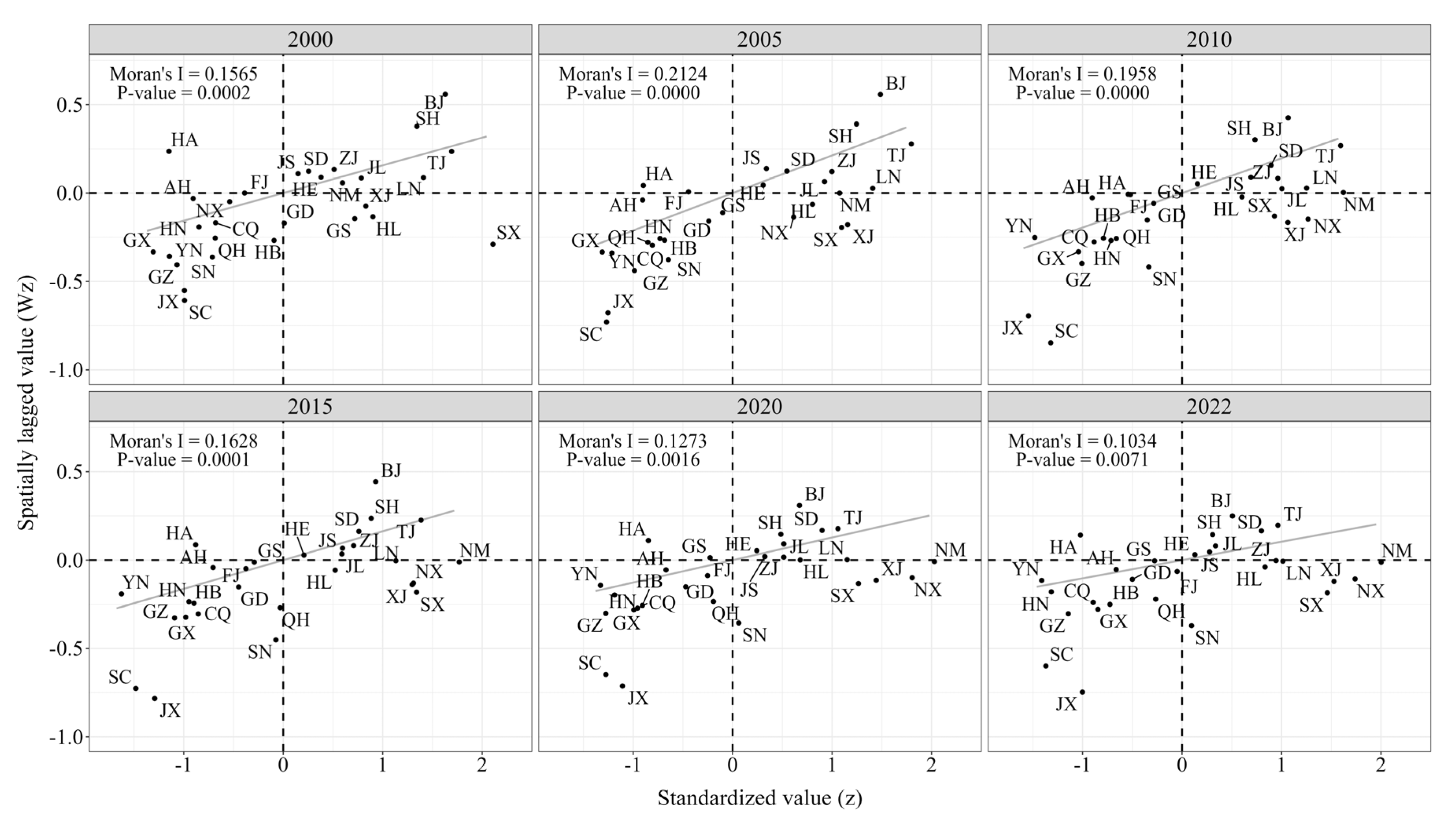
4.2. Spatial Autocorrelation Analysis

The Moran’s I index results are presented in

Table 4. Global Moran’s index of carbon emissions from Chinese household consumption.

Year	Moran’s Value	Z-Score	p-Value
2000	0.1565	3.7184	0.0002
2001	0.1759	4.0705	0.0000
2002	0.1907	4.3585	0.0000
2003	0.1926	4.3911	0.0000
2004	0.201	4.5558	0.0000
2005	0.2124	4.7630	0.0000
2006	0.2043	4.6053	0.0000
2007	0.2018	4.5520	0.0000
2008	0.2015	4.5465	0.0000
2009	0.1868	4.2717	0.0000
2010	0.1958	4.4477	0.0000
2011	0.1954	4.4476	0.0000
2012	0.1837	4.2328	0.0000
2013	0.1758	4.0680	0.0000
2014	0.1702	3.9632	0.0001
2015	0.1628	3.8223	0.0001
2016	0.152	3.6159	0.0003
2017	0.1284	3.1582	0.0016
2018	0.1547	3.6650	0.0002
2019	0.1373	3.3400	0.0008
2020	0.1273	3.1527	0.0016
2021	0.1231	3.0773	0.0021
2022	0.1034	2.6933	0.0071

. According to the Global Moran index of carbon emissions from household consumption in China, all indices exceed 0 and are significant at the 1% significance level, suggesting that provinces with high (or low) carbon emissions exhibit a clustered development trend, demonstrating a notable spatial positive correlation. Simultaneously, during the study period, the Global Moran index exhibits a fluctuating downward trend, decreasing from 0.1565 in 2000 to 0.1034 in 2022, indicating a gradual weakening of spatial interaction between provinces with similar carbon emissions. However, overall, these provinces remain in a state of significant agglomeration.

According to Figure 1, the spatial agglomeration effect of China’s consumption-based carbon emissions is mainly manifested as high–high agglomeration and low–low agglomeration. In 2000, the difference in the number of provinces within the high–high agglomeration area and the low–low agglomeration area was relatively minor. Specifically, ten provinces, namely Beijing, Shanghai, Tianjin, Liaoning, Jilin, Inner Mongolia, Zhejiang, Hebei, Shandong, and Jiangsu, were distributed in the high–high agglomeration area, exhibiting relatively high levels of carbon emissions, which were mirrored by their neighboring provinces. Conversely, ten provinces, namely Ningxia, Chongqing, Hunan, Qinghai, Shaanxi, Guangxi, Yunnan, Guizhou, Jiangxi, and Sichuan, were situated in the low–low agglomeration area, characterized by relatively low levels of carbon emissions, which were also reflected in their neighboring provinces. Over time, as of 2022, the number of provinces within the high–high agglomeration area decreased, while the number of provinces in the low–low agglomeration area increased, albeit with minimal fluctuation. Specifically, in 2022, nine provinces, namely Tianjin, Shandong, Beijing, Shanghai, Jilin, Hebei, Jiangsu, Zhejiang, and Liaoning, were located in the high–high agglomeration area. Conversely, eleven provinces, namely Sichuan, Jiangxi, Guizhou, Hunan, Yunnan, Chongqing, Guangxi, Hubei, Anhui, Guangdong, and Qinghai, were in the low–low agglomeration area. From 2000 to 2022, while the number of provinces categorized as high–high (H-H) and low–low (L-L) clusters exhibited temporal fluctuations, their spatial distribution maintained relative stability. This pattern is primarily attributed to H-H clusters persistently concentrating in economically advanced eastern coastal regions, where industrial structures dominated by the service sector and advanced manufacturing industries have driven elevated household consumption levels, consequently resulting in larger levels of carbon emissions. L-L clusters remain prevalent in less developed central and western regions, where lower household consumption levels and fewer carbon-intensive economic activities contribute to relatively smaller levels of carbon emissions.

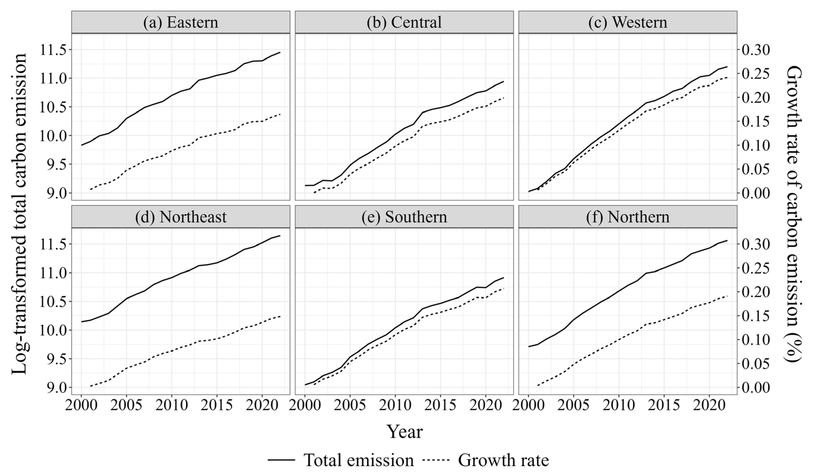
4.3. Time Series Characteristics

The household carbon emissions in China are presented in Figure 2. China’s household consumption of carbon emissions demonstrates an upward trajectory overall, with 2013 emerging as a critical inflection point. Post-2013, emission growth exhibited a significantly accelerated phase, followed by a deceleration in the growth rate while maintaining cumulative increases. Notably, the ascending pattern persisted despite moderated annual growth intensities in the post-2013 phase.

From a regional perspective, each region’s total carbon emissions and growth rates align relatively closely with those observed nationwide. In 2000, the carbon emissions of residents across various regions, ranked from highest to lowest, were the following: northeast (Figure 3d) > east (Figure 3a) > south (Figure 3e) > central (Figure 3b) > north (Figure 3f) > west (Figure 3c). By 2022, with minor adjustments, the ranking of carbon emissions from residents’ consumption, from highest to lowest, was the following: northeast > south > east > west > central > north. Regarding growth rates, the western region exhibited the fastest growth, whereas the northeastern region demonstrated the slowest growth. This disparity may be attributed to the increased investment and accelerated economic development in the western region, facilitated by the Western Development Strategy and the construction of the Silk Road Economic Belt. Consequently, this has fueled an improvement in residents’ consumption levels, which has increased energy consumption and carbon emissions. In contrast to the western region, the population growth in the northeastern region may have been relatively sluggish, and the consumption structure may have been more stable. Consequently, this has mitigated the additional carbon emissions from population growth and consumption upgrading.

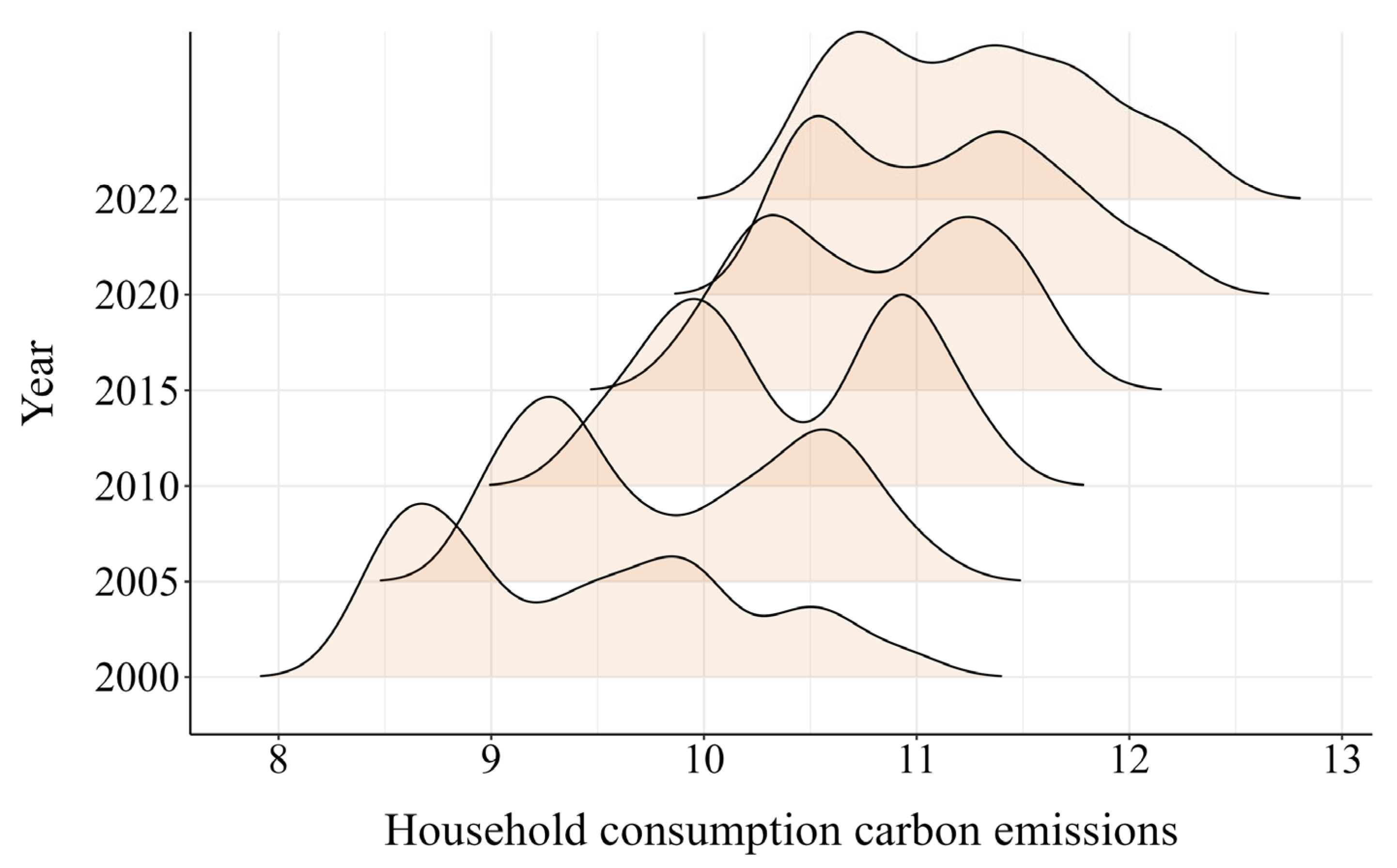
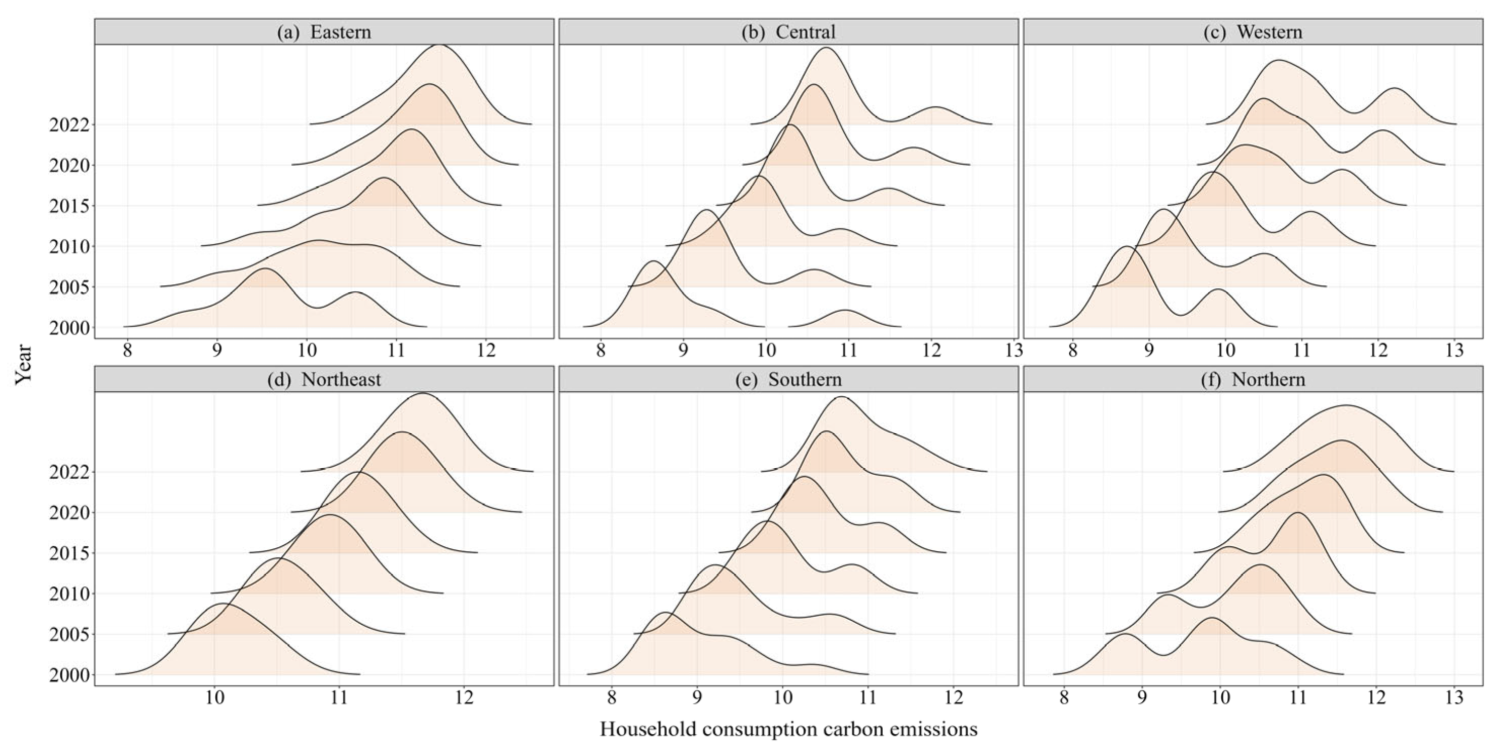
4.4. Dynamic Evolution Characteristics

Regarding the methodological framework developed by Fu et al. [30], this study employed a visualization strategy based on Kernel Density Estimation to elucidate the dynamic evolutionary characteristics of the distribution of carbon emissions across China. Figure 4 illustrates the national-level dynamic evolution. Relative to the baseline period, the distribution curve exhibits a progressive rightward shift post-2000, despite a temporary rebound in 2022. Cumulatively, household carbon emissions demonstrate an ascending trajectory at the national level. Analysis of peak elevation reveals continuous growth throughout the observation period, though the growth rate decelerates after 2010. By 2022, kurtosis reaches its peak value, accompanied by a contraction in distribution width. Notably, a bimodal distribution emerges in 2005, 2010, 2015, and 2020, which gradually transitions to a unimodal pattern. This shift reflects diminishing provincial disparities in household carbon emissions, indicating reduced polarization and revealing dynamic convergence trends in regional emission profiles. This phenomenon primarily stems from the Chinese government’s recent implementation of emission reduction policies, notably the “Dual Carbon” goals and region-specific environmental initiatives. These measures have facilitated dynamic convergence in the national distribution of carbon emissions.

Figure 5a illustrates the distribution and evolutionary traits within the eastern region. Throughout the observation period, the distribution curve in the east exhibits a gradual increase in peak height, while the width of the primary peak undergoes a progressive narrowing. This signifies a gradual reduction in the regional disparity of carbon emission levels among residents in the eastern region. The centroid of the density function undergoes a gradual rightward displacement, albeit with a deceleration in the pace of this shift over time, indicating a gradual increase in the carbon emission levels of residents in the eastern region. This is mainly because the eastern region has a developed economy, a higher level of income, and a stronger consumption capacity, leading to a higher level of carbon emissions. However, with the development of the economy and the improvement of residents’ awareness of environmental protection, the eastern provinces have gradually optimized their energy consumption structure and reduced their dependence on high-carbon energy, narrowing progressively the regional gap in carbon emission levels.

Figure 5b depicts the distribution and evolutionary characteristics in the central region. Overall, during the sample investigation period, there is no notable variation in the width and height of the density function. The central region’s centroid of the distribution curve gradually shifts to the right over time, indicating an overall upward trend within this region. Secondly, a right tail phenomenon persists in the central region throughout the initial and final time points. The plausible reason for this is that Shanxi, as a prominent coal-producing province in China, consumes significant amounts of coal resources, which objectively contributes to an increase in the direct carbon emissions of Shanxi residents.

Figure 5c illustrates the distribution and evolutionary traits in the western region. The centroid of the kernel density function shifts rightward, accompanied by an increase in width and a decrease in the prominence of the primary peak. It signifies an upward trend in the western region. In contrast, the absolute disparity in consumption-based carbon emissions among diverse provinces tends to broaden. Regarding distribution extension, the western region exhibits a right-tailed pattern during the observation period, with the curve in the tail region progressively flattening over time. It indicates a gradual widening of the spatial discrepancy among regional provinces. A plausible explanation lies in the substantial economic development disparities among provinces. Provinces with advanced economic levels, such as Chongqing and Sichuan, exhibit relatively higher residential consumption capacity and standards, potentially leading to higher carbon emissions. Conversely, less developed provinces may have lower levels of carbon emissions stemming from household consumption. Furthermore, the region exhibits heterogeneous energy consumption structures, with certain provinces, such as Neimenggu, relying heavily on high-carbon energy sources. This dual effect of uneven economic progression and diversified energy portfolios directly contributes to elevated household consumption carbon emissions, thereby exacerbating regional emission disparities within the Western territorial system.

Figure 5d illustrates the distribution and evolutionary traits in the northeastern region. The centroid of the kernel density function shifts rightward, accompanied by a slight narrowing in width. The height of the primary peak exhibits a trend of an “initial increase followed by a decrease”; however, compared to 2000, the height of the primary peak still exhibits a notable increase. It signifies an upward trend in the overall level, with a tendency for the absolute difference among regional provinces to diminish. No tailing phenomenon is observed regarding scalability, indicating the absence of significant gradient differences within the region during the sample observation period. A plausible explanation lies in China’s implementation of the “Revitalize the Northeast” policy, which has facilitated inter-regional infrastructure equalization and public service homogenization. These measures have effectively mitigated intra-provincial development disparities, thereby gradually narrowing carbon emission differentials in household consumption patterns alongside economic restructuring processes.

Figure 5e illustrates southern regions’ distribution and evolutionary characteristics. The centroid of the kernel density function shifts to the right, accompanied by a significant narrowing in width. The height of the primary peak displays a trend of an “initial increase followed by a decrease”. However, compared to 2000, the height of the primary peak still exhibits a notable increase, suggesting an upward trend in the overall level. Additionally, the absolute difference among southern provinces decreases. Regarding distribution extensibility, a tailing phenomenon is observed during the 2000 observation period, which dissipates by 2022. It indicates the absence of significant gradient differences as of 2022. This phenomenon may be attributable to the spillover effects from core economic hubs like the Guangdong–Hong Kong–Macao Greater Bay Area (GBA) and the southern Yangtze River Delta (YRD) region. Driving the coordinated development of neighboring provinces has contributed to the gradual convergence of the carbon emission levels of residential consumption.

Figure 5f illustrates northern regions’ distribution and evolutionary characteristics. The centroid of the kernel density function shifts to the right, accompanied by a significant narrowing of its width. The height of the primary peak exhibits a trend of an “initial increase followed by a decrease”. However, compared to 2000, the height of the primary peak still demonstrates a notable increase. This indicates that the overall level rises and the absolute difference among provinces decreases. In terms of distribution extensibility, no tailing phenomenon is observed, suggesting the absence of significant gradient differences within the northern region throughout the sample observation period. This phenomenon is mainly because the Beijing–Tianjin–Hebei coordinated development strategy promotes cross-regional resource sharing and institutional coordination. The level of household consumption carbon emission should converge under the strategic policy framework.

5. Convergence Analysis of Carbon Emissions from Chinese Household Consumption

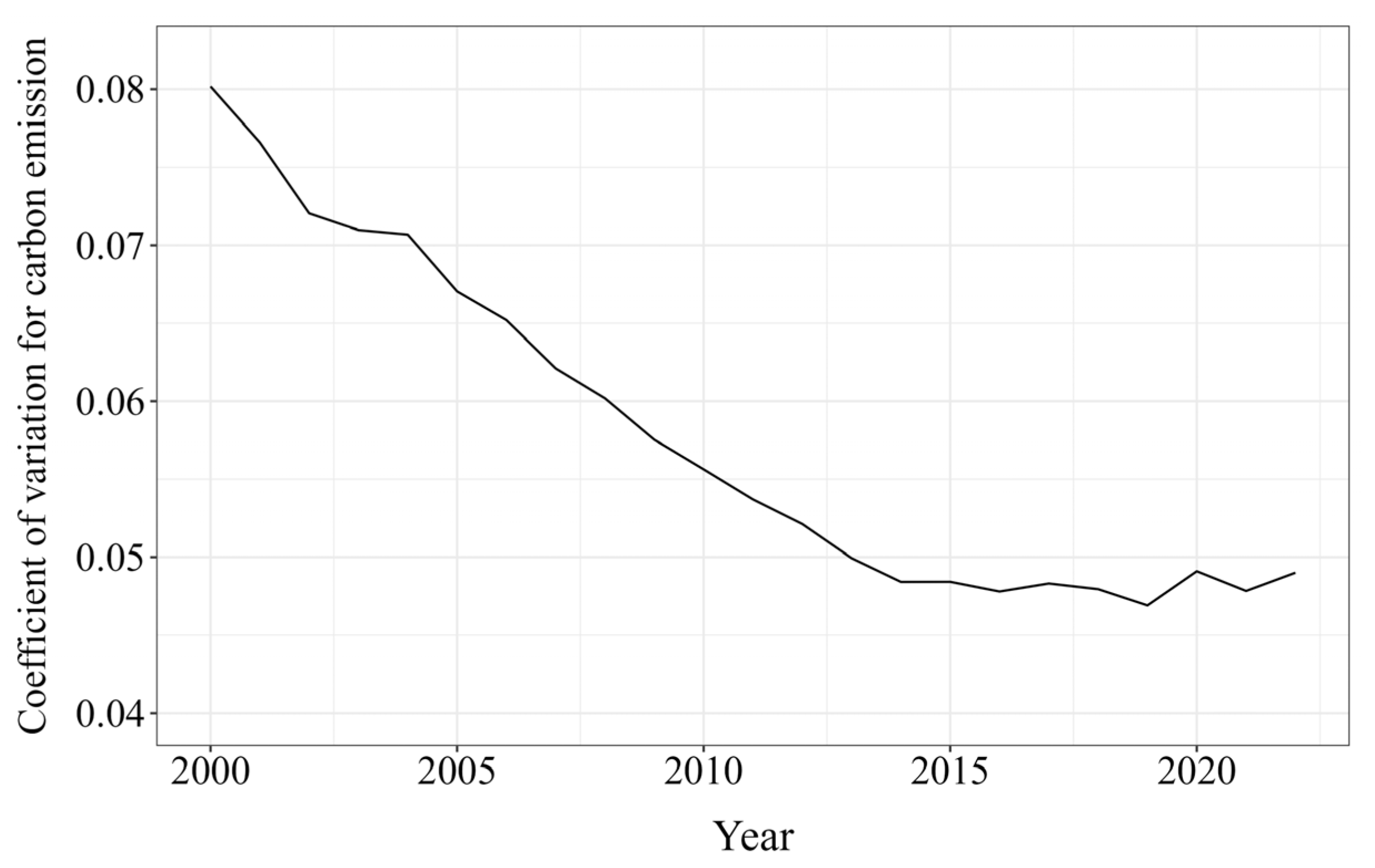
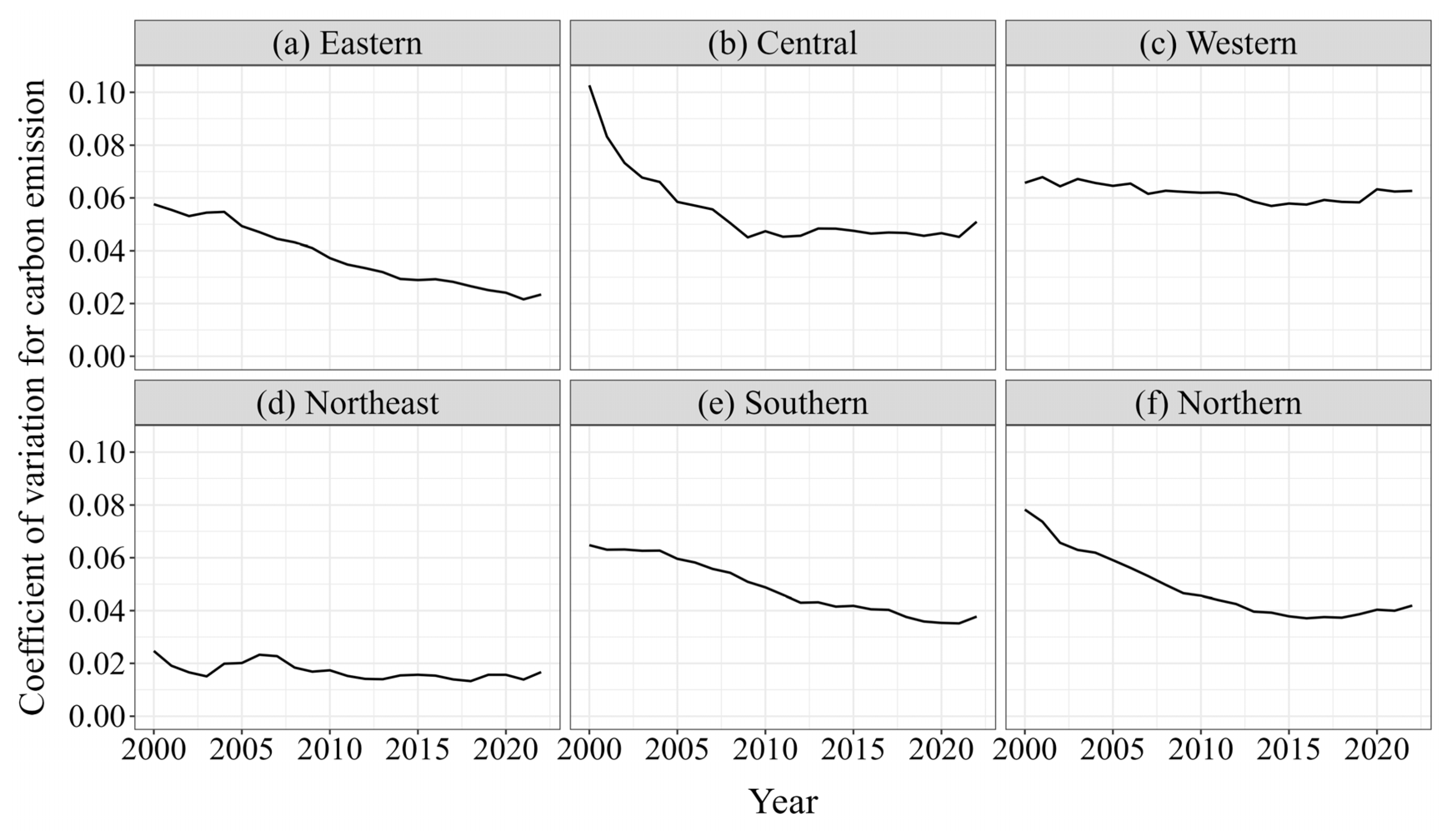
5.1. σ Convergence

Figure 6 illustrates the dynamic trend of the coefficient of variation for household consumption carbon emissions over the investigation period. From an evolutionary perspective, there is a discernible downward trajectory in the variability of household consumption-related carbon emissions at the national level, decreasing from 0.08 in 2000 to 0.05 in 2022. This trend signifies an annual average decline of 1.8%. This observation indicates a notable convergence nationwide, accompanied by a reduction in the dispersion among provinces, with the emission disparities gradually narrowing over time. This convergence phenomenon is primarily attributed to the unified implementation and reinforcement of national policies and regulations, such as energy conservation and emission reduction policies and the establishment of a carbon emission trading market, which have prompted provinces to adopt consistent measures in carbon emission management. Meanwhile, regional economic coordinated development and urbanization progress have driven technological advancement, the optimization of energy structure, enhanced public environmental awareness, and shifts in consumption patterns, collectively fostering the convergence of household consumption carbon emissions nationwide.

Figure 7 depicts the dynamic trend of the coefficient of variation for residents’ consumption-based carbon emission levels across various regions. Regionally, the coefficient of variation in both the eastern and central regions exhibited notable downward trends. Specifically, in the eastern region (Figure 7a), the coefficient decreased from 0.0576 in 2000 to 0.027 in 2022, reflecting an average annual decline of 2.7%. Similarly, it decreased from 0.1026 in 2000 to 0.0229 in 2022, with an average annual reduction of 2.29% in the central region (Figure 7b). That of the southern region (Figure 7e) saw a decline from 0.0648 in 2000 to 0.019 in 2022, averaging an annual decrease of 1.9%, while that of the northern region (Figure 7f) decreased from 0.0783 in 2000 to 0.0211 in 2022, with an average annual decline of 2.1%. In contrast, the coefficient of variation for residents’ consumption carbon emissions in the western region (Figure 7c) remained relatively stable, fluctuating around 0.062, and in the northeastern region (Figure 7d), it fluctuated around 0.017. These findings indicate that significant σ convergence was observed in China’s four major regions: the central, eastern, southern, and northern regions. However, the evolution of regional differences in consumer carbon emission levels in the western and northeastern regions did not demonstrate notable convergence. Notably, the convergence rate in the eastern region was markedly higher than that in the central region, and the convergence rate in the northern region significantly exceeded that in the southern region, suggesting a clear “catch-up” effect.

5.2. Absolute β Convergence

The Wald, LR, LM, and Hausman test models were used to select the optimal model for analyzing β convergence across the national level and the eastern, central, western, northeastern, southern, and northern regions [31]. The results presented in

Table 5. Absolute β convergence of carbon emissions from Chinese household consumption.

	Nationwide	Eastern	Central	Western	Northeastern	Southern	Northern
	(1)	(2)	(3)	(4)	(5)	(6)	(7)
Model	SEM	SEM	SDM	OLS	OLS	SEM	SEM
β	−0.5443 ***	−0.1292 ***	−0.2336 ***	−0.017 **	−0.0164	−0.0441 ***	−0.0585 ***
ρ/λ	0.878 ***	0.3747 ***	0.6289 ***	-	-	0.5377 ***	0.4236 ***
Cons.	-	-	-	0.2747 ***	0.2465 **	-	-
σ2_e	0.0452 ***	0.0041 ***	0.0044 ***	-	-	-	-
Convergence rate	3.57%	0.63%	1.21%	0.08%	-	0.21%	0.27%
LM-error	58.102 ***	17.756 ***	9.365 ***	0.024	0.674	30.062 ***	4.652 **
LM-lag	51.342 ***	15.75 ***	5.711 ***	0.034	0.629	27.792 ***	2.059
Robust-LM-error	7.356 ***	3.047 *	12.128 ***	0.039	0.644	3.522 *	5.552 **
Robust-LM-lag	0.596	1.041	8.474 ***	0.048	0.600	1.252	2.958 *
Hausman test	−12.38	11.39 ***	53.93 ***	49.47 ***	3.89 **	23.96 ***	−23.15
Wald-error	45.90 ***	7.89 ***	29.19 ***	21 ***	0.22	11.67 ***	26.32 ***
Wald-lag	223.60 ***	11.61 ***	51.87 ***	29.42 ***	0.24	18.16 ***	47.2 ***
LR test (SEM-SDM)	52.28 ***	8.63 ***	39.06 ***	27.03 ***	0.22	13.66 ***	37.63 ***
LR test (SAR-SDM)	84.03 ***	11.19 ***	42.13 ***	27.62 ***	0.24	17.47 ***	43.87 ***
Individual fixed effects	YES	YES	YES	YES	YES	YES	YES
Time fixed effects	YES	YES	YES	YES	YES	YES	YES
R2	0.0425	0.075	0.0529	0.0216	0.243	0.0524	0.0604
Obs.	609	189	126	242	66	273	336

Notes: * p < 0.10, ** p < 0.05, *** p < 0.01. The Hausman test statistics yield a negative value in columns (1) and (7). Through simulation analysis, this article referred to Lian et al. and identified that the primary reason for this outcome was the failure to satisfy the fundamental assumption of the random-effects (RE) model, namely, Corr(x_it, u_i) = 0. Consequently, fixed-effects (FE) models were employed [32]. The same is below.

indicate that the spatial lag coefficient at the national level is 0.878, which is statistically significant at the 1% significance level. It signifies the presence of absolute β convergence in national household consumption carbon emission levels, with a convergence rate of 3.57%. In other words, over time, the growth in the level of carbon emissions from residential consumption will eventually converge to the same steady state level, with provinces with lower levels of carbon emissions from residential consumption growing faster compared to provinces with higher levels of carbon emissions from residential consumption.

From a regional perspective, the convergence coefficient β demonstrates spatial absolute β convergence in the eastern, central, southern, and northern regions, whereas the western region exhibits general absolute β convergence. In contrast, the spatial lag coefficient in the northeastern region fails to pass the significance test, displaying divergent characteristics. Regarding convergence speed, the central region boasts the highest rate at 1.21%, followed by the eastern region at 0.63%, the northern region at 0.27%, the southern region at 0.21%, and the western region at 0.08%. This implies that the central region experience a more rapid convergence rate, whereas the eastern, western, southern, and northern regions converge at slower rates.

5.3. Conditional β Convergence

The conditional convergence of household carbon emissions was analyzed using control variables such as travel convenience, urbanization, pollution control capacity, economic development, labor quality, industrial structure, and industrialization level. The regression results (

Table 6. Conditional β convergence of carbon emission from Chinese household consumption.

	Nationwide	Eastern	Central	Western	Northeastern	Southern	Northern
	(1)	(2)	(3)	(4)	(5)	(6)	(7)
Model	SDM	OLS	SDM	OLS	OLS	SEM	SEM
β	−0.6478 ***	−0.023 **	−0.2412 ***	−0.0296 ***	−0.0203	−0.0337 **	−0.0624 ***
Wx	0.6553 ***	-	0.4063 ***	-	-	-	-
ρ/λ	0.289 ***	-	0.6519 ***	-	-	0.4937 ***	0.3877 ***
σ2_e	0.0414 ***	-	0.0034 ***	-	-	0.0051 ***	0.0075 ***
Convergence rate	4.74%	0.11%	1.25%	0.14%	-	0.16%	0.29%
LM-error	53.921 ***	16.123 ***	11.966 ***	0	0.579	27.869 ***	5.424 **
LM-lag	42.359 ***	15.407 ***	7.61 ***	0.068	1.056	25.235 ***	1.425
Robust-LM-error	16.987 ***	1.146	7.612 ***	2.072	0.874	4.218 **	16.058 **
Robust-LM-lag	5.425 **	0.43	3.256 *	2.14	1.201	1.583	12.059 ***
Hausman test	36.8 ***	−31.77	7.66	30.72 ***	134.53 ***	76.64 ***	53.76 ***
Wald-error	48.48 ***	7.8	34.04 ***	20.52 ***	21.49 ***	18.01 **	35.06 ***
Wald-lag	252.27 ***	10.1	60.91 ***	27.25 ***	22.64 ***	25.05 ***	60.26 ***
LR test (SEM-SDM)	70.14 ***	8	41.74 ***	25.74 ***	19.33 **	21.39 ***	50.1 ***
LR test (SAR-SDM)	95.92 ***	9.75	48.20 ***	25.75 ***	19.36 **	23.86 ***	55.19 ***
Individual fixed effects	YES	YES	YES	YES	YES	YES	YES
Time fixed effects	YES	YES	YES	YES	YES	YES	YES
R2	0.0384	0.0908	0.0381	0.0476	0.0261	0.0183	0.0171
Obs.	609	198	126	242	66	273	336
Travel convenience	−0.0011	0.0015	0.0041	−0.0028	0.0033	−0.0034	−0.0001
Urbanization level	0.0009	−0.0001	0.001	0.0008	0.0014	−0.0007	0.0001
Pollution control	−0.0127	−0.0066	0.0069	0.002	−0.0091	0.0021	0.0039
Economy	−0.0051	−0.0016	.0035	−0.0087	−0.0194	0.0159*	0.0064
Labor	−0.0973	0.0139	−0.0352	−0.0289	0.0138	0.1347 **	0.0395
Industrial structure	−0.1849 ***	0.0105	0.0641	0.0662	0.0306	0.0386	0.0183
Industrialization level	0.3208	0.2566	0.5628	0.492	−0.1017	0.6081 **	0.062
Cons.	-	0.2414	-	0.3994	0.4528	-	-

Notes: * p < 0.10, ** p < 0.05, *** p < 0.01. The Hausman test statistics yield a negative value in column (2). Consequently, fixed-effects (FE) models were employed.

) indicate significant negative convergence coefficients across most regions except the northeast. Specifically, convergence is significant at the 1% level in the national, central, western, and northern regions and at the 5% level in the eastern and southern regions. This suggests that carbon emissions in these areas are converging toward region-specific steady-state levels, largely due to the coordinated implementation of national environmental policies, such as energy conservation measures and the carbon trading system.

Convergence speeds increase notably in the national, central, western, and northern regions after accounting for control variables but slow in the eastern and southern regions. The northeast remains divergent. Spatial spillover effects are present in the national and central regions, where carbon emissions are positively influenced by neighboring provinces. Similarly, significant positive spatial autoregressive coefficients in the national, central, southern, and northern regions support the presence of spatial linkages in emissions, reflecting broader patterns of regional integration through trade, mobility, and technology diffusion. Notably, the central region, as a hub for industrial relocation, has enhanced cross-regional connectivity, while the southern and northern regions show evidence of policy coordination and technology sharing among provinces with similar environments.

At the national level, industrial structure negatively affects convergence, suggesting that regional disparities in industrial composition—between high-emission secondary sectors and cleaner tertiary sectors—hinder uniform emission reductions. In the south, however, economic development, labor quality, and industrialization significantly promote convergence. These factors support the adoption of low-carbon technologies, cleaner energy use, and environmentally conscious consumption patterns. Other control variables do not yield significant effects, and their roles warrant further investigation.

6. Discussion

This study develops a comprehensive analytical framework for examining the spatiotemporal evolution and convergence of household consumption-based carbon emissions, using provincial-level panel data from China. This framework offers a replicable empirical model for investigating global carbon mitigation pathways, particularly valuable for developing economies. The study draws on foundational databases such as the China Statistical Yearbook and China Energy Statistical Yearbook, which provide systematically organized longitudinal datasets that facilitate robust transnational benchmarking. The analysis is grounded in two critical dimensions: standardized accounting for direct energy consumption and the carbon emission factor method for indirect emissions. This integration of multi-source data offers a methodological reference for establishing national-level carbon accounting systems targeting residential consumption patterns worldwide, contributing to broader sustainability efforts.

While the current study focuses on aggregate provincial-level emissions, future research could benefit from incorporating a more nuanced approach, such as one analyzing per capita energy consumption. This would offer a more precise metric for assessing regional energy-use efficiency and the lifestyle characteristics driving emissions. By shifting from aggregate to per capita emission accounting, researchers could gain deeper insights into the spatiotemporal variations and convergence mechanisms of consumption-based carbon footprints across regions.

Moreover, carbon footprint analysis, which integrates greenhouse gas emissions from human activities, holds significant potential for future inquiries. Investigating provincial disparities in residential carbon footprints within China, in particular, could shed light on the underlying factors contributing to regional emission differences and provide valuable data to guide future mitigation efforts. This approach would not only refine our understanding of regional emissions but also highlight areas where targeted policy interventions could be most effective in reducing carbon footprints, thus supporting national and global sustainability goals.

7. Conclusions and Policy Implications

7.1. Conclusions

This paper examines how household carbon emissions have changed over time and across regions in China, using data from 29 provinces between 2000 and 2022. It asks whether regional differences matter in shaping these emission patterns. To answer this, this study applies a range of methods that capture both the distribution of emissions across space and how these patterns shift over time. These include techniques for measuring inequality, identifying geographic clustering, and tracking whether provinces are becoming more similar or more different in their carbon emissions. The aim is to understand not only where emissions are highest or lowest but also whether regions are converging toward common outcomes or continuing along divergent paths.

Findings reveal persistent high–high and low–low spatial agglomeration patterns, shaped by economic development, policy coordination, and proximity. Over time, high-emission clusters have slightly contracted, while low-emission zones have modestly expanded, reinforcing a stable spatial distribution. Nationally and across most regions, household emissions have risen, though absolute disparities have narrowed in all but the central and western regions. Relative disparities remain, especially within regions. Convergence trends are observed in the east, central, south, and north, while divergence persists in the northeast. Spillover effects, especially in the central region, highlight strong interprovincial linkages driven by market and energy integration. Spatial absolute and conditional β convergence indicates varied rates and directions of adjustment across regions. Industrial structure inhibits convergence nationally, while economic development, labor quality, and industrialization help reduce disparities. Overall, this study highlights the importance of spatially differentiated, policy-responsive carbon governance for managing household emissions and supporting national sustainability objectives.

7.2. Policy Implications

Effective carbon governance in China requires regionally differentiated and cooperative strategies aligned with long-term sustainability goals. First, building interprovincial carbon reduction alliances can support technological collaboration, policy coordination, and data sharing. Clearly defined responsibilities within these alliances can reduce free-riding and enhance collective impact, particularly in areas with strong spatial spillovers.

Second, carbon policies should be tailored to regional industrial structures, resources, and environmental capacities. High-emission regions must adopt stricter targets and advance low-carbon technologies, while low-emission regions can consolidate gains while supporting green growth. Such tailored approaches improve both efficiency and sustainability.

Third, policies should reflect regional comparative advantages: the east can promote green consumption through carbon markets; the central region should balance industrial growth with emissions control; and the western and northern areas can leverage renewable energy and urban hubs. The northeast requires structural reform to overcome divergence linked to legacy industries.

Finally, enhancing public awareness and societal participation is vital. Governments should promote environmental education and foster behavioral change through community engagement. A collaborative framework involving government, businesses, and households can foster innovation, green lifestyles, and participatory governance—key pillars for long-term, sustainable carbon reduction.

References

1. Zhou, H. Statistical calculation of carbon emission consumed by Chinese residents. Enterp. Econ. 2022, 41, 72–81. [Google Scholar]
2. Fu, W.; Li, L.; Wu, L.; Luo, M. Research progress and future prospects on carbon emissions from household consumption: Knowledge map analysis based on CiteSpace. Ecol. Econ. 2024, 40, 208–217. [Google Scholar]
3. Gao, P.; Yue, S.; Chen, H. Carbon emission efficiency of China’s industry sectors: From the perspective of embodied carbon emissions. J. Clean. Prod. 2021, 283, 124655. [Google Scholar] [CrossRef]
4. Feng, X.; Zhao, Y.; Yan, R. Does carbon emission trading policy has emission reduction effect?—An empirical study based on quasi-natural experiment method. J. Environ. Manag. 2024, 351, 119791. [Google Scholar] [CrossRef] [PubMed]
5. Borozan, D. European institutional quality and carbon emissions: Convergence club analysis. Struct. Change Econ. Dyn. 2024, 71, 646–657. [Google Scholar] [CrossRef]
6. Shi, P.; Huang, Q. Assessing the evolution and convergence of energy-related carbon emission efficiency in the Yangtze River Economic Belt. Process Saf. Environ. Prot. 2024, 191, 1684–1695. [Google Scholar] [CrossRef]
7. Ren, X.; Xiao, Y.; Xiao, S.; Jin, Y.; Taghizadeh-Hesary, F. The effect of climate vulnerability on global carbon emissions: Evidence from a spatial convergence perspective. Resour. Policy 2024, 90, 104817. [Google Scholar] [CrossRef]
8. Akram, V.; Rath, B.N.; Sahoo, P.K. Club convergence in per capita carbon dioxide emissions across Indian states. Environ. Dev. Sustain. 2024, 26, 19907–19934. [Google Scholar] [CrossRef]
9. Basso, H.S.; Dimakou, O.; Pidkuyko, M. How consumption carbon emission intensity varies across Spanish households. Ser.-J. Span. Econ. Assoc. 2024, 15, 95–125. [Google Scholar] [CrossRef]
10. Lian, Y.; Lin, X.; Luo, H.; Zhang, J.; Sun, X. Distribution characteristics and influencing factors of household consumption carbon emissions in China from a spatial perspective. J. Environ. Manag. 2024, 351, 119564. [Google Scholar] [CrossRef]
11. Pang, Q.; Xiang, M.; Zhang, L.; Chiu, Y.-H. Indirect carbon emissions from household consumption of middle-income groups: Evidence from Yangtze River Economic Belt in China. Energy Sustain. Dev. 2023, 76, 101280. [Google Scholar] [CrossRef]
12. Su, S.; Ding, Y.; Li, G.; Li, X.; Li, H.; Skitmore, M.; Menadue, V. Temporal dynamic assessment of household energy consumption and carbon emissions in China: From the perspective of occupants. Sustain. Prod. Consum. 2023, 37, 142–155. [Google Scholar] [CrossRef]
13. Cao, Q.; Kang, W.; Xu, S.; Sajid, M.; Cao, M. Estimation and decomposition analysis of carbon emissions from the entire production cycle for Chinese household consumption. J. Environ. Manag. 2019, 247, 525–537. [Google Scholar] [CrossRef] [PubMed]
14. Chen, J.; Lin, Y.; Wang, X.; Mao, B.; Peng, L. Direct and indirect carbon emission from household consumption based on LMDI and SDA model: A decomposition and comparison analysis. Energies 2022, 15, 5002. [Google Scholar] [CrossRef]
15. Jiang, L.; Ding, B.; Shi, X.; Li, C.; Chen, Y. Household energy consumption patterns and carbon emissions for the megacities-evidence from Guangzhou, China. Energies 2022, 15, 2731. [Google Scholar] [CrossRef]
16. Wang, Z.; Yang, L. Indirect carbon emissions in household consumption: Evidence from the urban and rural area in China. J. Clean. Prod. 2014, 78, 94–103. [Google Scholar] [CrossRef]
17. Liu, J.; Murshed, M.; Chen, F.; Shahbaz, M.; Kirikkaleli, D.; Khan, Z. An empirical analysis of the household consumption-induced carbon emissions in China. Sustain. Prod. Consum. 2021, 26, 943–957. [Google Scholar] [CrossRef]
18. Lian, Y.; Lin, X.; Luo, H.; Niu, Y.; Zhang, J. Empirical research on household consumption carbon emissions and key impact factors in urban and rural China. Environ. Sci. Pollut. Res. 2023, 30, 62423–62439. [Google Scholar] [CrossRef]
19. Peng, S.; Wang, X.; Du, Q.; Wu, K.; Lv, T.; Tang, Z.; Wei, L.; Xue, J.; Wang, Z. Evolution of household carbon emissions and their drivers from both income and consumption perspectives in China during 2010–2017. J. Environ. Manag. 2023, 326, 116624. [Google Scholar] [CrossRef]
20. Wang, J.; Hui, W.; Liu, L.; Bai, Y.; Du, Y.; Li, J. Estimation and influencing factor analysis of carbon emissions from the entire production cycle for household consumption: Evidence from the urban communities in Beijing, China. Front. Environ. Sci. 2022, 10, 843920. [Google Scholar] [CrossRef]
21. Ma, X.W.; Wang, M.; Lan, J.K.; Li, C.-D.; Zou, L.-L. Influencing factors and paths of direct carbon emissions from the energy consumption of rural residents in central China determined using a questionnaire survey. Adv. Clim. Change Res. 2022, 13, 759–767. [Google Scholar] [CrossRef]
22. IPCC. IPCC Guidelines for National Greenhouse Gas Inventories; Cambridge University Press: Cambridge, UK, 2006. [Google Scholar]
23. Liu, X.; Wang, X.; Song, J.; Wang, H.; Wang, S. Indirect carbon emissions of urban households in China: Patterns, determinants and inequality. J. Clean. Prod. 2019, 241, 118335. [Google Scholar] [CrossRef]
24. Li, S.; Ji, L.; Wang, Y.; Zhou, X.; Wang, X.; Jiang, S.; Sun, Q. Can China’s carbon generalized system of preferences reduce urban residents’ carbon emissions? Evidence from a quasi-natural experiment. J. Environ. Manag. 2024, 362, 121222. [Google Scholar] [CrossRef]
25. Wei, Y.; Liu, L.; Fan, Y.; Wu, G.; Fang, B.; Guo, J.; Han, Z.; Jiao, J.; Liang, Q.; Liao, H. China Energy Report (2008): CO2 Emissions Research; Science Press: Beijing, China, 2008. [Google Scholar]
26. Fu, Y.; Ma, S.; Song, B. Differences in consumption carbon emissions between urban and rural residents in China and influencing factors: An empirical analysis based on panel data. Inq. Into Econ. Issues 2016, 10, 43–50. [Google Scholar]
27. Chen, Y.; Gai, Q. The lmpact of the “Comprehensive Two-Child” Comprehensive Two-Child” Policy on Household Consumption Carbon Emissions. Consum. Econ. 2025, 41, 33–47. [Google Scholar]
28. Sun, L.; Wang, Q.; Zhou, P.; Cheng, F. Effects of carbon emission transfer on economic spillover and carbon emission reduction in China. J. Clean. Prod. 2016, 112, 1432–1442. [Google Scholar] [CrossRef]
29. Wang, S.; Huang, Y.; Zhou, Y. Spatial spillover effect and driving forces of carbon emission intensity at the city level in China. J. Geogr. Sci. 2019, 29, 231–252. [Google Scholar] [CrossRef]
30. Fu, Y.; Zhu, Y. The dynamic evolution, regional differences and convergence of agricultural product market segmentation in China. Stat. Res. 2024, 41, 18–32. [Google Scholar]
31. Guan, X.; Lu, X.; Wen, Y. Is China’s natural gas consumption converging? Empirical research based on spatial econometrics. Energies 2022, 15, 9448. [Google Scholar] [CrossRef]
32. Lian, Y.; Wang, W.; Ye, R. The efficiency of Hausman test statistics: A Monte-Carlo investigation. J. Appl. Stat. Manag. 2014, 33, 830–841. [Google Scholar]
Figure 1. Local Moran’s I scatter plot.
Sustainability 17 04064 g001
Figure 2. Time series characteristics of changes in carbon emissions levels of nationwide household consumption.
Sustainability 17 04064 g002
Figure 3. Time series characteristics of changes in household carbon emissions levels among regions.
Sustainability 17 04064 g003
Figure 4. Kernel density map of nationwide household consumption carbon emissions.
Sustainability 17 04064 g004
Figure 5. Kernel density map of carbon emissions of household consumption in regions.
Sustainability 17 04064 g005
Figure 6. The σ convergence of carbon emissions from nationwide household consumption.
Sustainability 17 04064 g006
Figure 7. The σ convergence of carbon emissions of household consumption in regions.
Sustainability 17 04064 g007