Impact of Shrinking Cities on Carbon Emission Efficiency in China

Abstract

The issue of urban carbon emission efficiency (CEE) has become a critical problem for global sustainable development, particularly in China, where the phenomenon of shrinking cities has emerged after rapid urbanization. Using panel data from 283 Chinese prefecture-level cities (2000–2016), we examine how urban shrinkage affects CEE through both direct and spatial spillover effects. Our findings show that urban shrinkage significantly improves CEE both directly and indirectly; when a city shrinks, it increases the local CEE by 0.0132%, while the contraction of adjacent cities enhances the local CEE by 0.0312%, leading to a total improvement of 0.0445%. However, the overall CEE in shrinking cities remains lower than the nationwide average, with values consistently below 0.5. The main determinants of CEE are GDP per capita and population size, which show significant direct positive effects but opposing regional spillover effects. These findings offer important insights for urban development policies and sustainable city management in the context of population decline.

1. Introduction

Carbon dioxide (CO₂) is a crucial greenhouse gas that is strongly linked to global warming [1]. Cities consume approximately 66% of the world’s energy and produce over 70% of global greenhouse gas emissions [2]. As a result, it is critical to evaluate cities’ carbon emission efficiency (CEE) to mitigate climate change and promote sustainable development. China has experienced tremendous urbanization over the preceding twenty years, with the urbanization rate rising from 30.09% in 2000 to 63.89% in 2020 [3]. However, these rapid and high urbanization rates pose a significant challenge to achieving carbon neutrality and carbon peaking in such a large developing country.

Notably, urban shrinkage has become a typical occurrence in China following periods of rapid urbanization [4]. Net population influx and natural population growth are the major causes of the increase in the urban population. However, due to regional economic imbalances, industrial restructuring, and demographic changes, the interregional mobility of urban labor has intensified [5,6]. The competition for population between cities has also intensified to obtain more net population inflows. Many rural residents have relocated to cities as a result of the country’s rapid urbanization [7]. These rural entrants have partially compensated for the population losses caused by the decline in the labor force in shrinking cities. However, China has entered a phase of high urbanization; in recent years, a phenomenon of counter-urbanization has even been present [8]. Rural migration may result in a decreasing supplemental population for cities. China’s low fertility rate in recent years has led to weak natural population growth and low or even zero newborn population growth. Therefore, the scope of China’s shrinking cities may extend even further.

When nations that urbanized early, such the United States and certain nations in Europe, began to experience shrinking cities, the notion of using the concept of shrink-ing cities as a unique viewpoint from which to examine urbanization began to gain public attention. The issue of shrinking cities has given rise to numerous worldwide projects, such as the EU-funded ‘Shrink Smart’ research project (funded by the Euro-pean Union’s Seventh Framework Programme, 2009–2012) and the EU COST Action on ‘Cities Regrowing Smaller’ (CIRES, European Cooperation in Science and Technology, 2009–2013). While sharing some common features with global cases, China’s shrinking cities present unique characteristics shaped by the country’s distinctive de-velopment context. Unlike Western countries where deindustrialization and suburban sprawl primarily drive urban shrinkage, China’s urban contraction is largely influ-enced by its massive internal migration patterns, rapid industrial restructuring, and the historical concentration of heavy industries in specific regions, particularly the northeast. These unique factors, combined with China’s ongoing urbanization process and economic transition, create a distinct pattern of urban shrinkage that warrants specific investigation.

While extensive research has examined CEE in Chinese cities, the environmental implications of urban shrinkage represent an emerging and understudied dimension. The distinct characteristics of shrinking cities—including declining population, changing industrial structure, and evolving resource utilization patterns—may lead to fundamentally different patterns of CEE than those observed in growing cities.

Domestic and international scholars have evolved their research on shrinking cities from the initial identification of socioeconomic impacts to exploring the multidimensional environmental effects and mechanisms of shrinking cities on land use [9], air pollution [10], and carbon emissions [4,11,12,13,14]. Among these environmental aspects, the relationship between shrinking cities and carbon emissions has increasingly become a focus of scholarly attention. Ribeiro et al. proposed a universal framework for studying the relationship between urban population and carbon emissions, finding that the impacts of urban population and density changes on carbon emissions are interrelated and dependent on their initial values. In the United States, the larger the city size, the greater the impact of population or density changes on carbon emissions. These studies on shrinking cities and carbon emissions have not only deepened our understanding of urban shrinkage phenomena but also provided new perspectives and insights for addressing global climate change and promoting sustainable development.

However, a debate still persists in the academic community regarding whether shrinking cities should be equated with urban depression [15]. In China, research on shrinking cities started later than that in developed countries. For a prolonged period, shrinking cities in China have not received adequate attention under the growth-oriented urban development model [16]. Specifically in the context of environmental impacts, according to Liu et al. [17], shrinking cities often have less energy-efficient household energy usage. Carbon dioxide emissions have been found to be steadily rising in a group of rapidly declining cities according to Xiao et al. [18]. Zeng et al. [19] noted that the CEE index of shrinking cities in northeastern China declines by 1.75% annually. Sun and Zhou [14] studied the influence of urban shrinkage on eco-efficiency in northeastern China and discovered that several mediating factors play a role but have opposing effects.

While various metrics such as carbon intensity, eco-efficiency, and energy efficiency can be used to evaluate urban environmental performance, we specifically focus on CEE because it provides a comprehensive measure of how effectively cities convert inputs into economic outputs while considering carbon emissions as an undesirable output. Unlike carbon intensity, which only considers the ratio of emissions to GDP, or energy efficiency, which focuses solely on energy consumption, CEE captures the overall efficiency of the urban production process in the context of carbon emissions, making it particularly relevant for evaluating the environmental impact of urban shrinkage.

CEE, which relates to the connection between inputs and outputs, is an essential metric for assessing the sustainability of cities. Two methods exist for carbon efficiency assessment: single-factor and full-factor methods. Focusing on only pollutant emission intensity is considered single-factor carbon efficiency assessment. This approach is straightforward with regard to calculation but overlooks the interrelationships between various components. In contrast, full-factor CEE considers multiple input and output factors, as well as the interactions between them. Evaluations of total-factor environmental efficiency have recently made substantial use of data envelopment analysis [20]. Using multiple inputs and outputs, this approach can handle complicated economic efficiency estimations while considering the potential for substitution among various natural resources and emissions and minimizing arbitrary weighting [21]. Many scholars use data envelopment analysis (DEA) to measure and compare CEE [22,23] at the national, provincial, municipal, and industry levels [24,25,26,27,28]. However, the diversity of cities at various stages of development is often underestimated.

Shrinking cities, however, differ significantly from growing cities in regard to their industrial structure, population density, and energy efficiency [18,29,30,31]. Although the literature has laid a strong foundation for this study, several critical gaps remain to be addressed. First, existing research on CEE in shrinking cities has been geographically limited, focusing primarily on specific regions such as northeastern China, making it difficult to draw comprehensive conclusions at the national level. Second, most studies rely on cross-sectional data or short-term observations, which may lead to biased estimates due to omitted variables and temporal variations. Third, the spatial dimension of CEE in shrinking cities has been largely overlooked, despite the well-documented spatial dependencies in both urban development and environmental performance. Fourth, the mechanisms through which urban shrinkage affects CEE remain unclear, particularly regarding the role of spatial spillover effects and regional heterogeneity.

Based on the above analysis, this study aims to address the following key scientific questions.

First, how does urban shrinkage affect CEE in China? While existing studies have examined CEE from various perspectives, the impact of urban shrinkage on CEE remains unclear, especially considering China’s unique urbanization context.

Second, what are the mechanisms through which urban shrinkage influences CEE? Given the complexity of urban systems, it is crucial to understand whether this influence operates through direct effects (such as industrial restructuring and population changes) or indirect effects (such as spatial spillovers).

Third, how do spatial factors mediate the relationship between urban shrinkage and CEE? Considering the significant regional disparities in China’s development, the spatial interaction effects between shrinking cities and their neighbors may play a crucial role in determining CEE outcomes.

To address these questions, we employ a super-efficiency SBM-DEA model with undesirable outputs to evaluate the CEE of 283 Chinese prefecture-level cities from 2000 to 2016. We chose this study period because 2000 marks the beginning of China’s rapid urbanization phase, while the data after 2016 are not included due to a significant change in the statistical caliber of urban electricity consumption data that occurred in 2017, which would affect the consistency and comparability of our CEE calculations. Furthermore, we utilize a spatial Durbin model to examine both the direct and indirect effects of urban shrinkage on CEE while taking into account spatial spillover effects.

The remainder of this paper is organized as follows. Section 2 introduces our methodology, including the super-SBM DEA model and spatial analysis methods, along with the data sources. Section 3 presents empirical results examining both temporal and spatial patterns of CEE in shrinking cities. Section 4 discusses the findings and their policy implications, and Section 5 concludes the study.

2. Methods and Materials

2.1. Super-SBM DEA Model with Undesirable Outputs

The relative effectiveness of several decision-making units with various inputs and outputs may be measured using the nonparametric efficiency analysis technique known as DEA [32]. The input of labor, capital, energy, and other components in the economic production process will not only result in the intended output, i.e., industrial items, but will also produce undesirable outputs, such as carbon dioxide, soot, and sewage. Traditional DEA models, however, consider only the desired outcomes of economic activity and disregard undesired outcomes [33]. We employ the super-efficiency SBM-DEA model for several key advantages over traditional DEA models. First, traditional DEA models cannot distinguish between efficient decision-making units with efficiency scores of 1, while the super-efficiency model allows for ranking among efficient units. Second, conventional DEA models typically ignore undesirable outputs, which is particularly problematic for environmental efficiency evaluation. The SBM-DEA model explicitly incorporates undesirable outputs such as CO₂ emissions. Third, this model addresses both the issue of slacks and the radial/non-radial problem simultaneously, providing more accurate efficiency measurements. Following these considerations, Tone [34] proposed the superefficient slack-based measure (SBM) of efficiency for DEA. This approach solves the slackness and radiality issues of variables and allows the differentiation and ranking of multiple efficient units. In this study, we use a superefficient SBM model that considers undesired outputs to evaluate the CEE of shrinking cities in China.

Assuming that there are n decision-making units (DMUs) in CEE, each of these units employs m inputs and generates s₁ desirable outputs and s₂ undesirable outputs. To represent these factors, we utilize three vectors: $x\in R^m$, $y^d\in R^{s_1}$, and $y^{ud}\in R^{s_2}$. Furthermore, we define the matrices X, Y^d, and Y^ud as follows:

$$\begin{array}{c}X=\left[x_1,x_2,\dots ,x_n\right]\in R^{m\times n} \end{array}$$

(1)

$$\begin{array}{c}{Y}^d=\left[y_1^d,y_2^d,\dots ,y_n^d\right]\in R^{s_1\times n}\end{array}$$

(2)

$$\begin{array}{c}{Y}^{ud}=\left[y_1^{ud},y_2^{ud},\dots ,y_n^{ud}\right]\in R^{s_2\times n}\end{array}$$

(3)

Assuming that X, Y^d, and Y^ud are greater than 0, the PPS can be defined as follows:

$$\begin{array}{c}P=\left\{\left(x,y^d,y^{ud}\right)\left|x\ge X\theta ,y^d\le \right.Y^d\theta ,y^{ud}\ge Y^{ud}\theta ,\theta \ge 0\right\}\end{array}$$

(4)

where $\theta$ represents the nonnegative intensity vector. The three inequalities in the P function represent the conditions under which the actual input level exceeds the frontier investment level, the actual desirable output level falls below the frontier desirable output level, and the actual undesirable output level exceeds the leading edge of the undesirable output level. Under the assumption of constant returns to scale, the following is the SBM model used for assessing DMU$\left(x_0, y_0^d,y_0^{ud}\right)$ to contend with undesirable outputs:

$$\begin{array}{c}\rho =min{\displaystyle \frac{1-\frac{1}{m}\sum _{i=1}^m\frac{s_i^{-}}{x_{i0}}}{1+\frac{1}{s_1+s_2}\left(\sum _{r=1}^{s_1}\frac{s_r^d}{y_{r0}^d}+\sum _{r=1}^{s_2}\frac{s_r^{ud}}{y_{r0}^{ud}}\right)}}, s.t.\left\{\begin{array}{c}{x}_0=X\theta +S^{-}\hfill \\ y_0^d=Y^d\theta -S^d\hfill \\ y_0^{ud}=Y^{ud}\theta +S^{ud}\hfill \\ S^{-}\ge 0,S^d\ge 0,S^{ud}\ge 0,\theta \ge 0\hfill \end{array}\right.\end{array}$$

(5)

where the slacks in inputs, desirable outputs, and undesirable outputs are denoted by $S=\left(S^{-},S^d,S^{ud}\right)$. $\rho$ represents the CEE value of DMU$\left(x_0, y_0^d,y_0^{ud}\right)$. The values m, s₁, and s₂ represent the numbers of factors for inputs, desirable outputs, and undesirable outputs, respectively. $\theta$ represents the intensity vector. If and only if $\rho =1$, which denotes that $S^{-}=0,S^d=0, \mathrm{a}\mathrm{n}\mathrm{d} S^{ud}=0$, in the presence of undesirable outputs, is DMU $\left(x_0, y_0^d,y_0^{ud}\right)$ SBM-efficient. If $0\le \rho <1$, the DMU needs to have its inputs and outputs upgraded. However, when more than one DMU has a $\rho$ value of 1, it is important to distinguish between them for the purposes of efficiency ranking and influence factor analysis. This work will integrate the research of Tone [35] into the basis of the SBM model to produce a super-SBM model with undesirable outputs, which is, in turn, utilized for assessing SBM-efficient DMUs to provide more precise efficiency evaluation values for efficiency analysis.

$${\rho }^{*}=min{\displaystyle \frac{\frac{1}{m}\sum _{i=1}^m\frac{\overline{x_i}}{x_{i0}}}{\frac{1}{S_1+S_2}\left(\sum _{r=1}^{S_1}\frac{{\overline{y}}_r^d}{y_{r0}^d}+\sum _{r=1}^{S_2}\frac{{\overline{y}}_r^{ud}}{y_{r0}^{ud}}\right)}};s.t.\left\{\begin{array}{c}\overline{x}\ge \sum _{j=1,\ne 0}^n{\theta }_j{x}_j\hfill \\ {\overline{y}}^d\le \sum _{j=1,\ne 0}^n{\theta }_j{y}_j^d\hfill \\ {\overline{y}}^{ud}\ge \sum _{j=1,\ne 0}^n{\theta }_j{y}_j^{ud}\hfill \\ \overline{x}\ge x_0,{\overline{y}}^d\le y_0^d,{\overline{y}}^{ud}\le y_0^{ud},{\overline{y}}^d\ge 0,\theta \ge 0\hfill \end{array}\right.$$

(6)

where ${\rho }^{*}$ represents the objective function, whose value can be more than 1.

2.2. Spatial Analysis

2.2.1. Spatial Autocorrelation

Nearby objects are more closely related to each other than distant objects [36]. China’s carbons emissions (CEs) may have a tendency to congregate [37,38,39]. Thus, we employ spatial autocorrelation to assess the level of geographical correlation between the observed data. Spatial autocorrelation is commonly tested using Moran’s I index [40,41]. Thus, this method can be used to measure the global and local spatial autocorrelation of CEE.

The global Moran’s I index examines the spatial aggregation of an entire spatial sequence ${\left\{x_i\right\}}_{i=1}^n$. It can be expressed as follows:

$$\begin{array}{c}{\mathrm{M}\mathrm{o}\mathrm{r}\mathrm{a}\mathrm{n}}^{\prime }\mathrm{s} I={\displaystyle \frac{{\sum }_{i=1}^n{\sum }_{j=1}^n{\omega }_{ij}\left(x_i-\overline{x}\right)\left(x_j-\overline{x}\right)}{S^2{\sum }_{i=1}^n{\sum }_{j=1}^n{\omega }_{ij}}}\end{array}$$

(7)

where ${\omega }_{ij}$ represents the (i, j) element of the spatial weight matrix, which is introduced to calculate the distance between areas i and j. $S^2={\displaystyle \frac{{\sum }_{i=1}^n{(x_i-\overline{x})}^2}{n}}$ represents the sample variance. ${\sum }_{i=1}^n{\sum }_{j=1}^n{\omega }_{ij}$ represents the aggregate of all spatial weights. The observed values of areas i and j observed values are represented by the variables $x_i$ and $x_j$, respectively. The mean of the measured values is represented by $\overline{x}$. The Moran’s I index is a metric used for spatial autocorrelation that expresses how geographically clustered or scattered observed values are. A value larger than 0 shows positive autocorrelation, meaning that high values are next to high values and low values are next to low values. A value less than 0 indicates negative autocorrelation, meaning that high values are next to low values. The range of this parameter extends from −1 to 1. The absence of spatial autocorrelation is observed when the Moran’s I index value is close to 0, which is considered a random spatial distribution. Importantly, regardless of the value of Moran’s I index, the data are considered to have no significant spatial autocorrelation when p > 0.05. The correlation coefficient between the observed values and their spatial lag can be used to understand Moran’s I index. The slope of the regression line that is fitted to the plot is identical to Moran’s I index in a Moran scatterplot.

Despite providing insights into the occurrence of geographical grouping, the global Moran’s I cannot identify the precise sites where such clustering takes place or determine whether there is a simultaneous coexistence of positive and negative spatial correlations. To address these limitations, further analysis is required using the local Moran’s I index. The local Moran’s I index is calculated as follows:

$$\begin{array}{c}{\mathrm{M}\mathrm{o}\mathrm{r}\mathrm{a}{\mathrm{n}}^{\prime }\mathrm{s} I}_i={\displaystyle \frac{\left(x_i-\overline{x}\right)}{S^2}}{\sum }_{j=1, j\ne i}^n{\omega }_{ij}\left(x_j-\overline{x}\right)\end{array}$$

(8)

where $I_i$ represents the local Moran’s I index value for a specific city i. If $I_i$ is positive, it means that the high (or low) value of region i is surrounded by other high (or low) values. However, if it is negative, it means that the high (or low) value of region i is surrounded by other low (or high) values.

2.2.2. Spatial Econometric Models

In classic linear regression models, data with spatial autocorrelation may result in inaccurate estimations of regression coefficients. As a result, we must analyze the variables that affect the data while taking the spatial correlation into account. By adding data from nearby locations, spatial regression models offer a way to increase the information set. Spatial regression models include a spatial lag vector W_y to account for the effects of the dependent variable in other areas since changes in the explanatory factors of one observation may impact the dependent variables of subsequent observations [42]. There are several varieties of spatial panel models, including the spatial lagged model (SLR), the geographic error model (SEM), and the spatial Durbin model (SDM), the uses of which are chosen based on whether the dependent variable or the error term has a geographic connection [43].

According to the SLR model, the explained variable of the neighboring spatial unit influences the explanatory variables of a particular spatial unit. The model can be represented as follows:

$$\begin{array}{c}{Y}_{it}=\rho \sum _{j=1}^N{W}_{ij}{y}_{jt}+\phi +X_{it}\beta +{\mu }_i+{\alpha }_t+{\epsilon }_{it}\end{array}$$

(9)

where $Y_{it}$ represents the dependent variable (CO₂ emission efficiency) for cross-sectional unit i at time t (i = 1,…, N; t = 1,…, T). The parameter ρ denotes the scalar spatial autoregressive parameter. The variable $\sum _{j=1}^N{W}_{ij}{y}_{jt}$ represents the interaction impact of the dependent variable $Y_{it}$ with the dependent variables $y_{jt}$ in nearby units, where $W_{ij}$ represents the i, jth element of a prespecified nonnegative N $\times$ N spatial weights matrix W. The spatial weight matrix W is constructed based on the geographic distance between cities i and j. We chose the geographic-distance-based approach because it better captures the continuous nature of environmental spillover effects and economic interactions between cities, which are not necessarily limited by administrative boundaries. This specification allows us to account for the varying intensities of spatial relationships based on the actual physical distance between cities.

$$\left\{\begin{array}{c}{W}_{ij}={\displaystyle \frac{1}{d_{ij}}}\left(when i\ne j\right)\\ W_{ij}=0 \left(when i=j\right)\end{array}\right.$$

(10)

where $d_{ij}$ represents the great circle distance between cities i and j. To ensure the robustness of spatial econometric analysis, we standardize the weight matrix by row, such that the sum of each row equals 1: $\sum W_{ij}$ = 1. This standardization helps interpret the spatial lag terms as weighted averages of neighboring observations. This matrix describes the spatial unit layout in the sample. $\phi$ represents the parameter for the constant term. $X_{it}$ represents a set of observations on explanatory variables such as per capita GDP, annual GDP growth rate, secondary industry rate, population, population density, built-up area, and local fiscal revenue. $\beta$ is a regression coefficient column vector. ${\mu }_i$ and ${\alpha }_t$ represent spatially and temporally specific effects, respectively. Finally, ${\epsilon }_{it}$ represents an independently and identically distributed error term for i and t, with a zero mean and variance of ${\sigma }^2$.

The SEM describes a situation in which an unobserved shock to city i is influenced by unobserved shocks in nearby areas. The model is described as follows:

$$\begin{array}{c}{Y}_{it}=\phi +X_{it}\beta +{\mu }_i+{\alpha }_t+u_{it}, { u}_{it}=\rho \sum _{j=1}^N{W}_{ij}{u}_{it}+{\epsilon }_{it}\end{array}$$

(11)

where $\rho$ is referred to as the spatial autocorrelation coefficient. According to the spatial weight matrix W and an idiosyncratic component ${\epsilon }_{it}$, the error term of unit i, $u_{it}$, is assumed to rely on the error terms of surrounding units j.

The spatial lag model is extended with spatially lagged independent variables in the SDM model. It is provided by the following:

$$\begin{array}{c}{Y}_{it}=\rho \sum _{j=1}^N{W}_{ij}{y}_{jt}+\phi +X_{it}\beta +\sum _{j=1}^N{W}_{ij}{X}_{ijt}\gamma +{\mu }_i+{\alpha }_t+{\epsilon }_{it}\end{array}$$

(12)

where $\gamma$ is a (K $\times$ 1) vector of spatial autocorrelation coefficients on the explanatory variables, and ρ denotes a scalar spatial autocorrelation coefficient on the dependent variables in this particular specification.

To choose the best model for this investigation, we use the methods outlined by Elhorst [43]. The results of various specification tests are presented in

Table 1. Model selection test results for the spatial econometric analysis of CEE.

Test		Indicator	Statistics (CEE)
LM test	SEM	Moran’s I	3.39 ***
		LM	264.79 ***
		R-LM	177.61 ***
	SLM	LM	87.18 ***
		R-LM	0.21
LR test	both to ind		145.32 ***
	both to time		4234.74 ***
Hausman test			−956.28
Wald test	SAR		51.42 ***
	SEM		36.77 ***
LR test	SAR		50.90 ***
	SEM		36.08 ***

Notes: *** indicates significance at the 1% level.

. Initially, we run Lagrange multiplier (LM) and robust LM tests to see if adding spatial effects, such as SLR or SEM, improves the model compared with that without spatial effects. Subsequently, the significance of the temporal and spatial effects is confirmed using the likelihood ratio test. Finally, the LR test is used to determine if the SDM collapses to either the SEM or SLR model. The spatial Durbin model is the model that best fits the data if both H₀: $\gamma =0$ and H₀: $\gamma +\rho \beta =0$ are disproved. On the other hand, the spatial lag model is the most suitable model if the initial null hypothesis cannot be ruled out and the robust LM tests support this. Furthermore, the spatial error model is the most appropriate model if the second null hypothesis cannot be ruled out and the robust LM tests also support its use. If neither of these requirements is fulfilled, i.e., if the robust LM tests imply the use of a different model than that suggested by the Wald/LR tests, then the spatial Durbin model should be used because it generalizes both the spatial error and spatial lag models.

We evaluate the spatial spillover effects of CEE after selecting the model. LeSage and Pace [42] caution that using point estimates from one or more spatial regression models to verify the existence of spatial spillovers may result in incorrect findings. The coefficient is part of the recursive computation of marginal effects. A more reliable basis for testing the hypothesis is a partial derivative interpretation of the effects of changes to the variables of various model specifications. The vector form of the spatial Durbin model can be expressed as follows:

$$\begin{array}{c}{Y}_{it}={\left(I-\rho W\right)}^{-1}\left(\beta X_t+W{X}_t\gamma \right)+{\left(I-\rho W\right)}^{-1}{\epsilon }_t^{*}\end{array}$$

(13)

where the error term ${\epsilon }_t^{*}$ contains intercept and error terms, and the matrix of the dependent variable’s partial derivatives in each unit regarding the kth explanatory variable $x_{ik}$(i = 1,…, N) in each unit at a specific time is as follows:

$${\left[{\displaystyle \frac{\partial Y}{\partial x_{1k}}}·{\displaystyle \frac{\partial Y}{\partial x_{Nk}}}\right]}_t={\left[\begin{array}{ccc}{\displaystyle \frac{\partial y_1}{\partial x_{1k}}}& \cdots & {\displaystyle \frac{\partial y_1}{\partial x_{Nk}}}\\ ⋮& \ddots & ⋮\\ {\displaystyle \frac{\partial y_N}{\partial x_{1k}}}& \cdots & {\displaystyle \frac{\partial y_N}{\partial x_{Nk}}}\end{array}\right]}_t={\left(1-\rho W\right)}^{-1}\left[\begin{array}{cccc}{\beta }_k& w_{12}{\theta }_k& \cdots & w_{1N}{\theta }_k\\ w_{21}{\theta }_k& {\beta }_k& \cdots & w_{2N}{\theta }_k\\ \cdots & \cdots & \cdots & \cdots \\ w_{N1}{\theta }_k& w_{N2}{\theta }_k& \cdots & {\beta }_k\end{array}\right]$$

(14)

The average of the matrix’s diagonal components, which is shown on the right side of Equation (14), represents the direct impact. It describes the whole effect of the local explanatory factors on the local explained variable. The average of the row sums or the column sums of the off-diagonal components of that matrix represents the indirect effect. The term ‘spatial spillover effect’ describes how nearby areas’ pertinent variables (X, Y) affect the focus region’s explained variable Y. It is possible to separate the indirect influence into two parts. The first part is the impact of the surrounding region’s explanatory variable X on the focal region’s explanatory variable Y. The second part is when a nearby region’s X has an impact on its own Y, which is subsequently communicated back into this domain’s Y via a closed-loop feedback mechanism. The sum of the direct and indirect impacts represents the overall effect.

2.3. Data Sources and Variable Selection

2.3.1. CO₂ Emission Efficiency

This study utilizes CEE as the dependent variable, which is calculated through the total factor carbon efficiency, incorporating input variables such as capital, labor, and energy. While various air pollutants affect environmental quality, we focus specifically on CO₂ emissions because this is the primary greenhouse gas driving global climate change [1]. China’s dominant source of CO₂ emissions is electricity production [44], and fixed asset investment has been identified as the primary contributor to emissions growth after the early 2000s, accounting for 61% and 71% of emissions growth from 2007 to 2010, respectively [45]. Considering the findings of previous research [46], we choose three key input variables that directly influence urban CO₂ emissions: fixed asset investment represents capital input and typically correlates positively with CO₂ emissions through infrastructure construction and industrial development; labor input (measured by the number of workers) reflects the scale of economic activities and their associated emissions; electricity consumption serves as the energy input indicator, directly linking to CO₂ emissions. We use electricity consumption data as China does not publish comprehensive urban energy consumption data. To maintain data uniformity, the study period is limited to 2000–2016, as urban electricity consumption data in the city statistical yearbook underwent significant adjustments in 2017 and later years. The output element is split into two categories, namely, desirable output, which is represented by GDP, and undesired output, which is represented by CO₂ emissions. The input-output factor data required to calculate the total factor carbon efficiency are as follows. The input-output factor data required to calculate CEE are shown in

Table 2. Descriptive statistics of input–output elements for the super-SBM DEA model.

Indicator	Variables	Unit	Obs	Mean	Std. Dev.	Min	Max
Input	Fixed asset investment	108 yuan	4811	613	895	5	12,090
	Labor force	104 person	4811	84	117	5	1729
	Electricity	108 kW·h	4811	66	121	1	1486
Desirable output	GDP	108 yuan	4811	1051	1659	18	19,918
Undesirable output	CO2 emission	104 ton	4811	2322	2656	48	26,891

Notes: The data related to assets and income are adjusted to constant 2000 prices. All GDP and fixed asset investment values in our dataset are positive, allowing for direct logarithmic transformation without any special handling required for zero or negative values. This is consistent with the nature of these economic indicators at the prefecture-level city scale.

.

2.3.2. Shrinking Cities

There is not yet a consensus on the definition of ‘shrinking cities’ among academics. While urban shrinkage can manifest in multiple dimensions, including economic decline, job market contraction, and infrastructure underutilization, a sustained decline in population serves as the primary indicator as it effectively captures these various aspects of urban shrinkage. Population decline often correlates strongly with and precedes other shrinkage indicators such as economic downturn and job losses. To mitigate potential demographic calibration biases, this study utilizes an urban contraction dummy variable to enhance the robustness of its findings [17]. This study uses the year 2000 as the base period by which to identify population changes in the 283 selected Chinese prefecture-level cities. Cities with an urban population smaller than that of the base period are designated as shrinking cities and assigned a value of 1 for the shrinking dummy variable. Conversely, cities with an urban population larger than that of the base period are classified as non-shrinking cities and assigned a value of 0 for the shrinking dummy variable.

2.3.3. Control Variables

Previous research has examined various factors that influence CO₂ emissions, such as affluence, lifestyle, and technology [29,47,48,49,50,51,52]. This study incorporates three dimensions of control variables: economic, demographic, and policy factors. Economic-level variables include GDP per capita (PerGDP), GDP growth rate (GDPR), and the share of secondary industries (Sec). Demographic-level variables include population (Pop) and population density (PopDen). The policy level includes variables such as built-up area (Area) and local fiscal revenue [53]. The data related to assets and income are adjusted to constant 2000 prices.

2.3.4. Data on the Variables

This research assesses the CEE of 283 Chinese prefecture-level cities, as well as the impact of shrinking cities, using panel data from between 2000 and 2016.

Table 3. Descriptive statistics of CEE and control variables for Chinese cities.

Variable	Description	Obs	Mean	Std. Dev.	Min	Max
CEE	Carbon emission efficiency	4811	0.38	0.17	0.08	2.67
Shrinking	Dummy variable	4811	0.07	0.26	0	1
PerGDP	Per capita GDP (ln)	4811	9.71	0.83	7.43	12.81
GDPR	Annual GDP growth rate (%)	4811	11.70	4.95	−19.38	109.00
Sec	Secondary industry/Total	4811	0.48	0.11	0.03	0.91
Pop	Population (ln)	4811	5.84	0.69	2.77	8.13
PopDen	Population density (ln)	4811	5.71	0.91	1.55	9.36
Area	Built-up area (ln)	4811	4.19	0.87	1.61	8.12
Rev	Local fiscal revenue (ln)	4811	12.56	1.48	7.20	17.63

presents the variables’ summary statistical data.

The data on CO₂ emissions utilized in this study are drawn from Tomohiro Oda’s Open-Data Inventory for Anthropogenic Carbon Dioxide (ODIAC) [53]. ODIAC is a worldwide emission data package with high geographic resolution that calculates CO₂ emissions from burning fossil fuels. To determine the worldwide geographic extent of fossil fuel CO₂ emissions, a combination of space-based nighttime light data and individual power plant emission/location characteristics is used. In studies pertaining to urban emission estimation, ODIAC provides a worldwide, monthly, high-resolution gridded data package for fossil fuel CEE at a 1-km $\times$ 1-km resolution. While ODIAC provides comprehensive coverage at 1 × 1 km resolution, it is worth noting that, like all global emission inventories, it may have limitations in capturing some small-scale emission sources. However, for our study of prefecture-level cities, these potential uncertainties are minimized as we focus on aggregate city-level emissions.

Data on the resident population of Chinese cities are typically available only from decennial census statistics. Therefore, due to the unavailability of continuous yearly panel data on the population of Chinese prefecture-level cities, this study employs year-end household registration population data to examine urban population decline. While prefecture-level analysis may not capture variations within cities (such as differences between urban cores and suburban areas), it represents the most appropriate spatial scale for our study because of the following: (1) it is the primary administrative level at which urban development policies are implemented in China, and (2) consistent and comparable data for key variables are only available at this level. Data on population size and other geographic and socioeconomic variables are obtained from China Statistical Yearbooks, the China City Statistical Yearbooks, and statistical yearbooks of provinces and prefecture-level cities. Missing data were minimal in our dataset, affecting less than 2% of the total observations. In these few cases, interpolation techniques were employed to supplement the information. Given the small proportion of missing values, this data-handling approach has negligible impact on our main findings.

3. Results

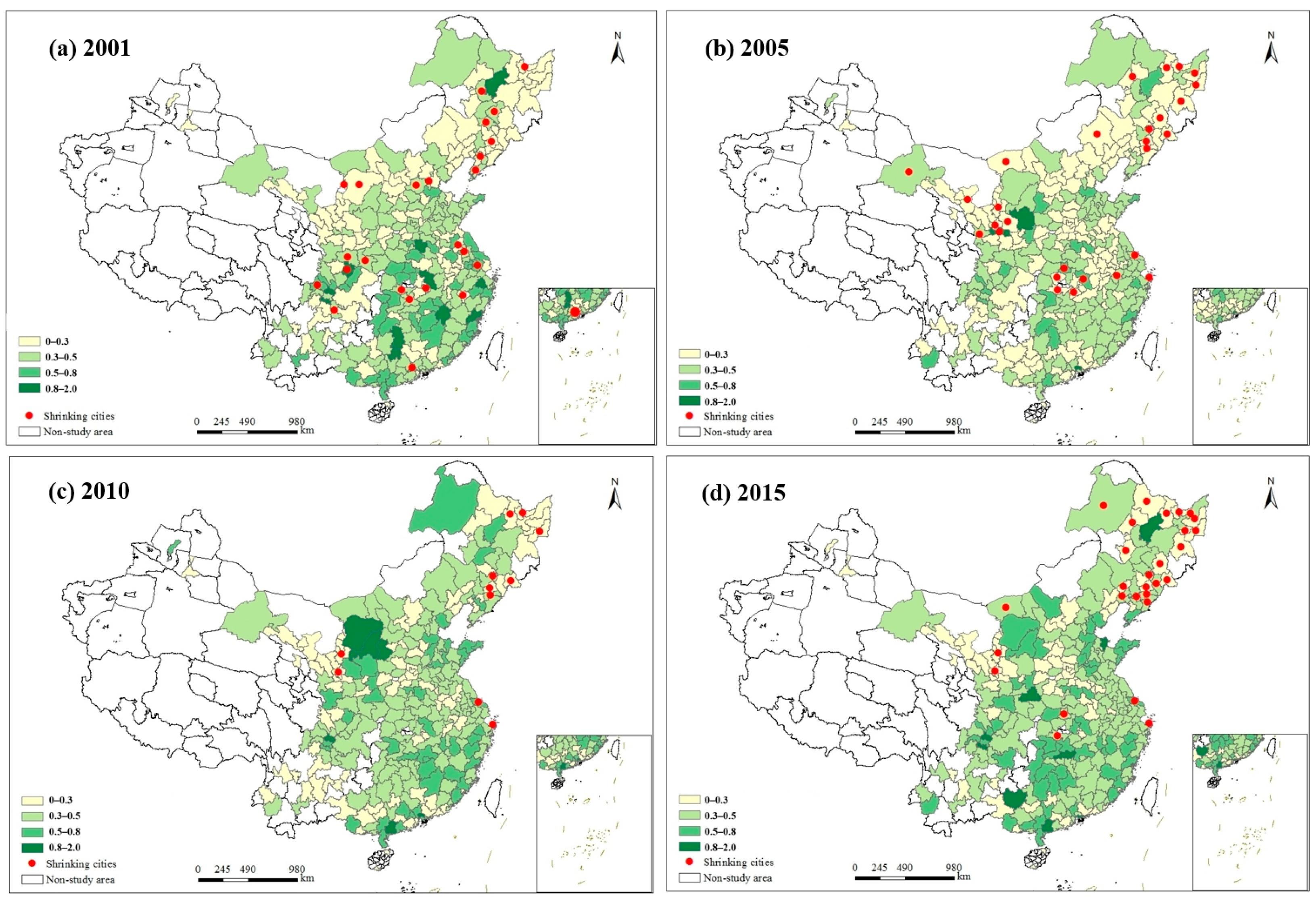
3.1. Temporal and Spatial Distribution of Urban CEE and Shrinking Cities

To illustrate the geographical patterns of urban efficiency and shrinkage, Figure 1 displays the spatial distribution of urban CEE and shrinking cities across China for four representative years: 2001, 2005, 2010, and 2015. Spatially, the distribution of China’s urban CEE presents a prominent pattern of high concentration along the eastern coast while demonstrating lower levels in the midwest and northeast regions. Such a pattern resembles the findings of Cai et al. [54], which highlight the presence of imbalanced low-carbon development across China. The total CEE levels in China did not significantly change during the study period, and mostly remained generally low in value.

From 2000 to 2016, the percentage of shrinking cities in China experienced fluctuations and increases, standing at 8.48%, 9.40%, 4.59%, and 9.89% in 2001, 2005, 2010, and 2015, respectively. Geographically, China’s shrinking cities are mainly found in the northeastern part of the country, with fewer cities located in the middle and western parts. By 2015, most shrinking cities had become concentrated in the northeastern region, comprising over 70% of the nation’s shrinking cities. The northeast region serves as China’s heavy industrial base and has encountered challenges such as industrial restructuring and overcapacity following the 2008 financial crisis. Additionally, the region has traditionally relied on industries such as coal production and forestry, which are now facing issues of resource depletion. As a result, these cities’ traditional industries are no longer able to sustain their economic growth, which is causing a steady decrease in the local population and substantial urban contraction.

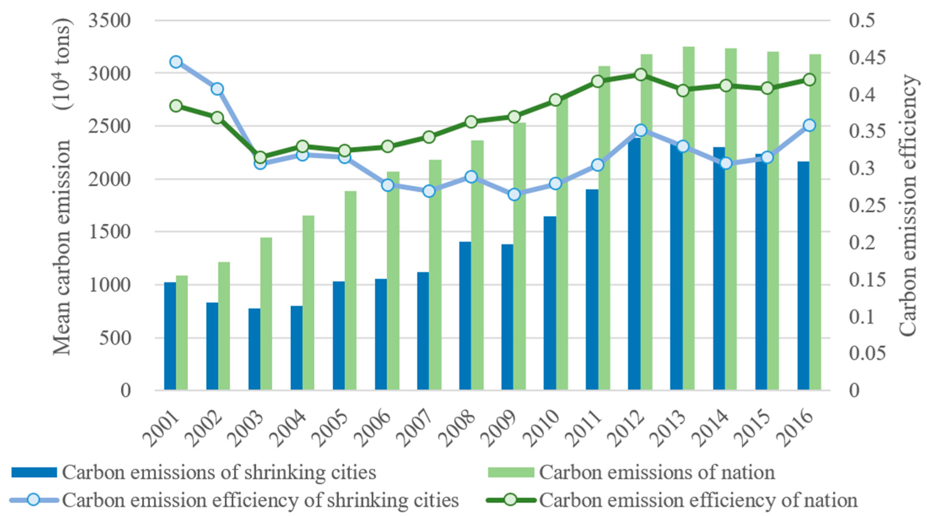
3.2. Urban CE and CEE of China

The evolution trends of the CEs and CEE of prefecture-level and shrinking cities in China are shown in Figure 2. The average CEs of cities nationwide follow a two-stage trend. The first stage, spanning from 2001 to 2013, is characterized by a rapid growth period, during which the average urban CO₂ emissions nearly tripled, growing at a high rate of 9.57% per year on average. The second phase, spanning from 2013 to 2016, is distinguished by a gradual fall in average CEs, with a 0.69% yearly decrease rate on average.

The nationwide trend of urban carbon emissions is different from the average CE of shrinking cities. Specifically, a brief decline in carbon emissions occurred in 2001–2004, with an average yearly decrease rate of 7.86%. The CEs of shrinking cities peaked in 2012, with a yearly rise of 14.61%. Notably, with China’s economic growth slowing, the CEs of contracting cities also entered a period of decline after 2012, with an average annual decrease of 2.47%.

Between 2001 and 2003, both national and shrinking cities exhibited a substantial decline in CEE. Following this period, urban CEE showed steady and consistent improvement from 2003 to 2013, albeit with a slight decline after 2013. In comparison, the CEE of shrinking cities displays a consistent trend at the national level, although it exhibits more significant fluctuations. It is noticeable that since 2006, the CEE of decreasing cities has consistently been lower than the national average.

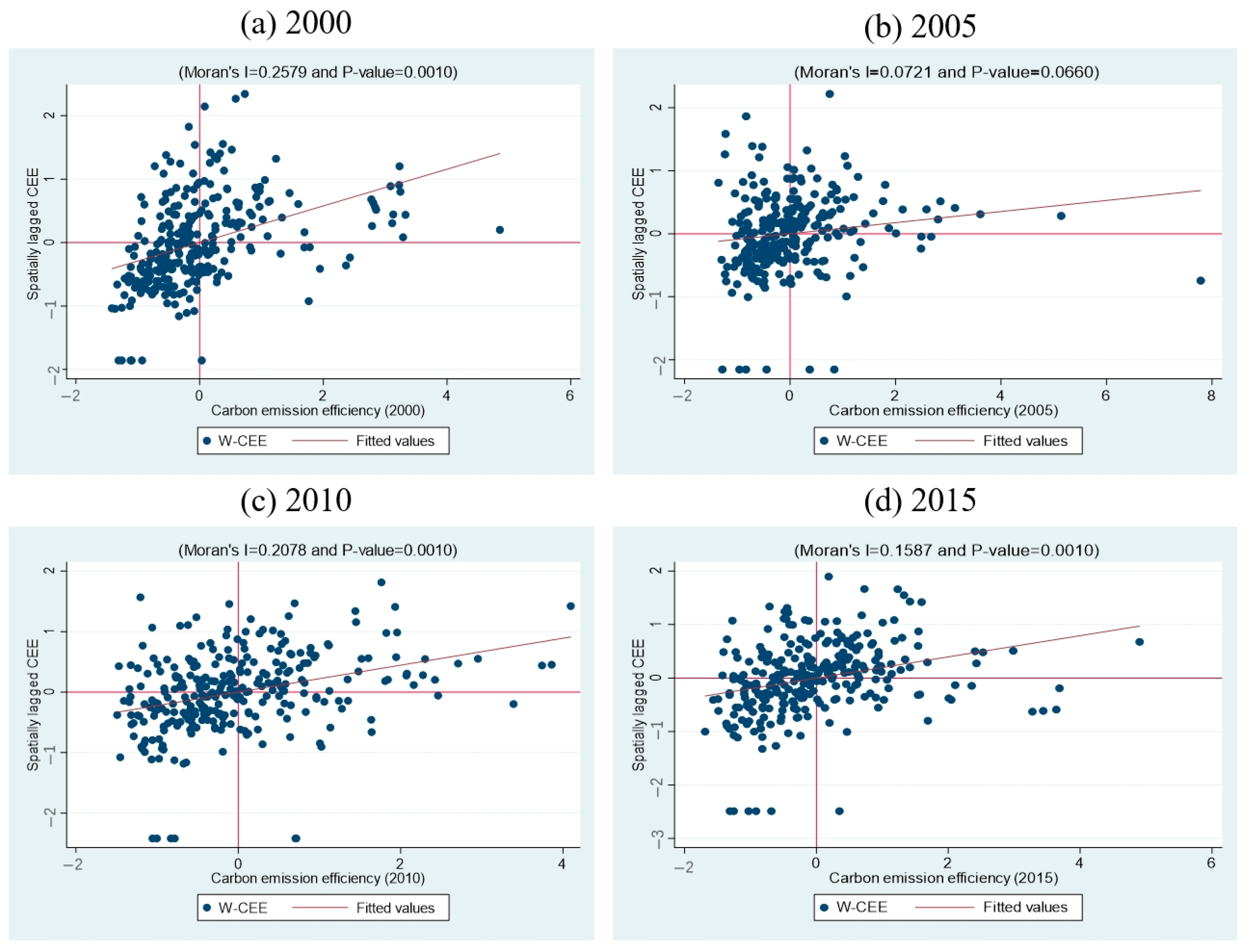
3.3. Spatial Autocorrelation of CEE

Using the spatial autocorrelation analysis method described in Section 2.2.1, the results of the global Moran’s I index are shown in

Table 4. Global Moran’s I test results for the spatial autocorrelation of CEE.

Year	I	z	p Value	Year	I	z	p Value
2000	0.26	6.56	0.00	2009	0.15	3.87	0.00
2001	0.26	6.68	0.00	2010	0.21	5.27	0.00
2002	0.27	6.84	0.00	2011	0.15	3.76	0.00
2003	0.25	6.31	0.00	2012	0.15	3.82	0.00
2004	0.24	5.98	0.00	2013	0.15	3.83	0.00
2005	0.07	1.94	0.05	2014	0.17	4.25	0.00
2006	0.17	4.41	0.00	2015	0.16	4.07	0.00
2007	0.21	5.20	0.00	2016	0.10	2.64	0.01
2008	0.17	4.25	0.00

and demonstrate a significant positive spatial autocorrelation of urban CEE across the years spanning from 2000 to 2016 at a level ranging from 1% to 10%. This signifies that the use of a spatial econometric model is better suited for statistical analysis than a conventional regression model.

The Moran scatter plot shown in Figure 3 depicts how urban CEE was distributed spatially in 2000, 2005, 2010, and 2015. CEE is shown on the horizontal axis. A positive spatial autocorrelation of CEE is indicated by the figure, which demonstrates that most cities are concentrated in the first and third quadrants. The spatial autocorrelation of CEE is especially high–high or low–low. That is, cities with high CEE tend to group together with other high-CEE cities, while cities with low CEE tend to cluster with other cities that have low CEE.

3.4. Spatial Panel Data Model Analysis

According to the model test findings shown in Table 1, the results of the Lagrange multiplier (LM) test and robust LM test reveal that the spatial lag model (SLR) and spatial error model (SEM) both outperform the model without spatial effects. The results of the likelihood ratio (LR) test show that both temporal and spatial effects are significant. Finally, the results of the LR test demonstrate that the spatial Durbin model (SDM) does not degenerate to either SLR or SEM. These outcomes indicate that the SDM model is the best match to the data; thus, this is the model that we utilize for the spatial econometric analysis of CEE.

Table 5. Spatial Durbin model results for direct and indirect effects on CEE.

	(1)	(2)	(3)	(4)	(5)
	Main Effect	W$\times$	Direct Effect	Indirect Effect	Total Effect
Shrinking	0.0119	0.0242 *	0.0132 *	0.0312 **	0.0445 **
	(1.5310)	(1.6814)	(1.6560)	(1.9740)	(2.5148)
PerGDP	0.2355 ***	−0.0685 ***	0.2340 ***	−0.0325 **	0.2015 ***
	(22.3587)	(−4.4420)	(23.3018)	(−2.0297)	(11.7708)
GDPR	−0.0007 **	−0.0015 **	−0.0008 **	−0.0019 ***	−0.0026 ***
	(−2.1269)	(−2.4555)	(−2.3086)	(−2.9041)	(−3.6604)
Sec	−0.1083 ***	−0.0293	−0.1101 ***	−0.0505	−0.1606 ***
	(−3.0282)	(−0.5481)	(−3.2283)	(−0.8322)	(−2.5969)
Pop	0.2201 ***	−0.1067 ***	0.2177 ***	−0.0814 *	0.1363 ***
	(11.1885)	(−2.6775)	(11.2228)	(−1.8682)	(2.8000)
PopDen	−0.0020	0.0083	−0.0010	0.0101	0.0091
	(−0.1772)	(0.3821)	(−0.0948)	(0.4047)	(0.3638)
Area	−0.0110 *	0.0246 **	−0.0102	0.0254 **	0.0152
	(−1.8507)	(2.1656)	(−1.6431)	(2.0931)	(1.0776)
Rev	−0.0496 ***	0.0259 ***	−0.0491 ***	0.0200 **	−0.0291 ***
	(−10.8271)	(3.4833)	(−11.0716)	(2.4368)	(−3.3528)
Obs	4811	4811	4811	4811	4811
Spatial rho	0.1649 ***
	(8.4149)

Notes: ***, **, and * are significant at the levels of 1%, 5%, and 10%, respectively. T statistics are in parentheses.

displays the SDM regression findings with the inclusion of control variables. Columns (1) and (2) show the calculated coefficients of the spatial lag factors. Spatial rho has a significantly positive value, showing the presence of spatial effects. It should be made clear that the estimated coefficient of the spatial lagged variables contributes to only the recursive computation of the marginal impact; it does not directly represent the spatial effect. In accordance with the methods suggested by [42], we use direct, indirect, and total effects to examine the impact of the explanatory factors on the explained variable CEE, as specified in Columns (3) to (5).

3.4.1. Effects of Shrinking Cities

Based on the spatial Durbin model outlined in Section 2.2.2, the estimated direct, indirect, and cumulative impacts of the main explanatory variable of shrinking on the explained variable of CEE are shown in Table 5, following the addition of control variables. The results show a significant positive direct effect coefficient in the third column at the 10% significance level. Specifically, when a city experiences shrinkage, the local CEE is elevated by 0.0132%. In the fourth column, it can be seen that the indirect effect of shrinking on CEE is also positive at the 5% significance level, implying that urban shrinkage has a positive spatial spillover effect. When a neighboring city experiences shrinkage, it increases the local CEE by 0.0312%.

The total effect of shrinking on CEE, which is presented in the fifth column, is estimated to be 0.0445 at the 5% significance level. This finding suggests that, as measured by the total factor productivity, urban shrinkage has a minor but significant positive influence on CEE. Notably, the direct, indirect, and total effects of urban contraction on CEE are all positive. These results indicate that although many Chinese cities are undergoing contraction, such contraction does not have a negative impact on China’s CEE. In contrast, urban shrinkage helps social resources flow and be distributed more logically, which significantly benefits CEE.

3.4.2. Effects of Control Variables

Urban shrinkage is one of the elements that affects CEE, according to the results shown in Table 5; however, other factors, including the economy, population, and policy, also have a significant influence on CEE.

The direct effects of the control variables suggest that GDP per capita and population size have a significant positive impact on CEE. Specifically, 1% increases in GDP per capita and urban population contribute to 0.234% and 0.2177% increases in CEE, respectively. Therefore, economic development and population size remain the primary drivers of CEE. On the other hand, the GDP development rate, secondary industry ratio, and local fiscal revenue display significant negative direct effects on CEE, with correlation coefficients of −0.0008, −0.1101, and −0.0491, respectively. Population density and built-up area do not significantly directly affect CEE.

Some control variables also have significant spatial spillover effects. For instance, the built-up area and local fiscal revenue of neighboring cities show significant positive spatial spillover effects on CEE, with an increase of 1% in these variables leading to a 0.0254% and 0.02% increase in local CEE, respectively. However, the GDP per capita, GDP development rate, and population size of adjacent cities have significant negative spatial spillover effects on CEE. To be more precise, each 1% increase in GDP per capita, GDP development rate, and population size of adjacent cities reduces CEE by −0.325%, −0.0019%, and −0.0814%, respectively. However, the share of secondary industry and population density do not exhibit a significant indirect effect, indicating that changes in these factors in nearby cities have little impact on local CEE.

4. Discussion

4.1. CEs and CEE of Chinese Cities

The trajectory of urban CEs in China has exhibited a remarkable pattern over the past two decades. Specifically, from 2001 to 2013, there was a large increase in CE, followed by a slow decrease from 2013 to 2016. Scholars have established that the rise in China’s export sector after its Word Trade Organization (WTO) membership began in 2001 played a pivotal role in this surge in carbon emissions [44]. The nation’s booming manufacturing industry, coupled with a surge in export demands, led to a substantial increase in CEs, as documented by Zhang et al. [55]. However, China’s economy has been in a period of slow development since 2013, which has helped to limit the rising trend of carbon emissions in major cities. Interestingly, shrinking cities recorded a temporary decrease in carbon emissions from 2001 to 2003, plausibly due to their low level of competitiveness in the international division of labor following China’s accession to the WTO. However, with the implementation of the ‘Western Development’ program in 2004, a slew of industrial firms were introduced to these shrinking cities in China’s western regions, resulting in a significant increase in carbon emissions, which peaked in 2012.

The current state of CEE in China’s prefecture-level and shrinking cities is a matter of concern, as indicated by the low average value of CEE, which does not exceed 0.5. This shows that the CEE of Chinese cities has much potential for improvement. Furthermore, the trend of national urban CEE is characterized by fluctuation and an overall increase. Notably, China’s WTO membership, particularly in its early phases, has positioned the nation at the bottom of the global supply chain, resulting in fast GDP growth fueled by labor-intensive, low-end manufacturing items. However, this has come at the cost of significantly increased CO₂ emissions from undesired outputs, which have ultimately resulted in a decline in carbon efficiency.

With the implementation of the Eleventh Five-Year Plan in 2006, China addressed the need to strike a balance between economic growth and environmental protection. The establishment of a target responsibility system for energy conservation and emission reduction, as well as the incorporation of energy consumption per unit of GDP into the comprehensive assessment system for economic and social development, was a key measure taken in holding local governments accountable for their efforts to conserve energy. While urban energy consumption decreased, CEE continued to rise, reaching a peak in 2012.

Our findings reveal that China’s shrinking cities continuously have lower CEE values than the national average for cities, which is a concerning issue. The causes of this discrepancy can be attributed to various factors at both the endogenous and exogenous levels. At the endogenous level, shrinking cities are mainly concentrated in China’s northeastern provinces, which are known for their heavy industry and resource-based economies. The results of the analyses conducted in Section 3.4.2 of this paper suggest that economic development, population size, and industrial structure play significant roles in determining CEE. Unfortunately, shrinking cities have a comparative disadvantage in regard to these aspects when compared with growing cities. Furthermore, at the exogenous level, China’s low-carbon regulations, such as the Low-Carbon City Pilot (LCCP) program, have been instrumental in improving CEE. Research has demonstrated that the LCCP program has significantly improved CEE [56,57]. However, the majority of cities with LCCP policies are concentrated in China’s eastern regions, while shrinking cities are mainly located in the northeast and midwest regions. Energy-intensive and polluting industries may migrate from LCCP cities to less-developed areas. In a bid to boost tax revenue and employment, governments in shrinking cities may offer incentives such as inexpensive land and lenient environmental policies to accommodate these industries, further exacerbating the gap with the national CEE.

4.2. Impacts of Urban Shrinkage on CEE

Urban shrinkage’s impacts on CEE in Chinese cities comprise a complicated and multidimensional problem, with varying regional effects and significant implications for national policy decisions. Although the CEE of shrinking cities is below the national average, urban shrinkage in China has been shown herein to have a significant positive direct, indirect, and total effect on CEE in terms of population change. In contrast, Zeng, Jin, Geng, Kang, and Zhang [19] studied the CEE of 14 northeastern Chinese cities and found that urban contraction has a negative effect on CEE. These different conclusions can be attributed to several factors. First, variations in study scope: Our nationwide analysis captures diverse urban contexts, while northeastern studies focus on a region characterized by heavy-industry- and resource-based economies. Second, methodological differences: Our incorporation of spatial effects reveals spillover benefits that may be missed in traditional analyses. Third, temporal context: The northeastern region experienced more severe and prolonged population loss, potentially leading to different economic and environmental dynamics compared with cities with moderate shrinkage. These contrasting findings highlight the complexity of urban shrinkage’s environmental impacts across different regional contexts.

Regarding the direct effects, urban shrinkage exerts a significant positive impact on local CEE through three main channels. First, the process of urban shrinkage promotes industrial structure optimization. As cities experience population loss and economic transformation, traditional high-energy-consuming and high-pollution industries gradually decline or relocate. This natural elimination process helps optimize the industrial structure, leading to reduced carbon emissions while maintaining economic output. For instance, many shrinking cities in northeastern China have seen their traditional heavy industries being replaced by more efficient and environmentally friendly sectors.

Building upon this industrial transformation, the second channel operates through population mobility and resource reallocation. When young and skilled workers migrate to more developed regions, they often acquire advanced knowledge and skills. Some of these workers eventually return to their home cities, bringing back new technologies and management practices that can improve production efficiency and reduce carbon emissions. This “brain circulation” effect is particularly evident in cities that have implemented policies to attract returning talents. Additionally, the reduced population pressure allows cities to allocate resources more efficiently and adopt more advanced production technologies.

The third channel, which is closely linked to both industrial transformation and population dynamics, involves more efficient resource utilization. The contraction of urban population and economic activities often leads to the consolidation and optimization of existing infrastructure and industrial facilities. For example, shrinking cities can concentrate their production activities in more efficient facilities while phasing out outdated ones. This consolidation process helps improve energy efficiency and reduce unnecessary carbon emissions. Moreover, the availability of vacant land and facilities provides opportunities for the development of renewable energy projects and green infrastructure, further contributing to improved CEE.

The suggestions can help guide national decisions about programs that aim to reduce carbon emissions and promote urban growth.

Regarding the direct effects, urban contraction exerts a significant positive correlation on local CEE. The process of urban development has been under constant pressure due to the regional and local economic transformations induced by globalization [58]. The supporting industries in a city have their own development cycle, which is characterized by employment opportunities and population influx during times of industrial prosperity and population outflow during times of economic downturns. In this regard, the population of a city changes in response to the cyclical rise and fall of its supporting industries. The decline of traditional industries in mining or manufacturing results in the economic contraction of a city or region, leading to a reduction in local economic output and employment opportunities [59]. However, this phenomenon also mitigates the environmental disruptions caused by the crude economic development model, which benefits the CEE of the region. Notably, urban construction in shrinking cities has slowed due to the redundant stock of buildings brought on by population out-migration. Empirical evidence indicates that the CEE related to China’s building industry is decreasing [60]. Therefore, urban contraction can also be seen to reduce the inefficient carbon emissions arising from the development of the building industry to some extent. While the desired output of GDP is reduced in shrinking cities, the undesired output of CO₂ emissions and input indicators (including labor, electricity consumption, and asset investment) are reduced even more. Consequently, from the perspective of total factor productivity, urban contraction is seen to optimize the local CEE.

In terms of indirect effects, CEE significantly benefits from the expansion of surrounding cities on a spatial level. With the encouragement of industrial upgrading in Chinese cities and the adoption of national low-carbon policies, industries with high energy consumption, high pollution, and low value added are being progressively phased out. The abolition of such backwards industries frees up a considerable quantity of excess labor, which goes to neighboring cities, resulting in population loss and contraction. Due to the lack of employment prospects in the surrounding contracting cities, young people and individuals with high levels of education are attracted to local areas, creating a talent-crowding-out effect that provides the labor needed for advanced services in the new economy. This phenomenon is particularly evident with the advent of high-speed rail in China, which has significantly reduced the time and economic costs of intercity transportation, exacerbating the brain drain from contracting cities [61].

Moreover, with the decline in the local economy, social capital investment also flows from contracting cities to neighboring cities, promoting economic development and generating greater economic output. Therefore, although these cities experience contraction, they create higher CEE than that found in areas with surplus labor staying in place due to the release of labor to neighboring cities and other efficient industries. This spillover effect is significant and positive, highlighting the importance of considering the impact of neighboring cities on local CEE.

These findings contribute to the broader theoretical debate on whether urban shrinkage can be ‘beneficial’ for environmental sustainability. While traditional urban theory often views shrinkage negatively, our results suggest that population loss might create opportunities for environmental improvement through industrial restructuring and resource optimization. However, this environmental benefit must be understood within China’s unique development context.

While our findings demonstrate a positive relationship between urban shrinkage and CEE in China, this pattern may differ in other international contexts. Chinese shrinking cities are unique in several aspects: they are experiencing shrinkage amid rapid national urbanization, maintain strong state intervention capabilities, and often possess substantial industrial bases. In contrast, shrinking cities in Europe (such as in Germany’s Ruhr region) or the United States (such as Detroit) typically face different institutional contexts and economic structures. These differences suggest that the positive effect of urban shrinkage on CEE might be partially attributable to China’s specific institutional and economic context. Future comparative studies could explore how different institutional arrangements and economic structures mediate the relationship between urban shrinkage and environmental performance.

4.3. Effects of Control Variables on CEE

Numerous academic studies have investigated the determinants of CEE. Economic development and population size continue to have a significant positive direct effect on CEE. Cities with higher per capita GDP tend to have undergone structural economic transformation and industrial upgrading, leading to the elimination of highly polluting and low-value industries and, ultimately, resulting in a higher level of urban CEE. Furthermore, during periods of massive rural-to-urban migration, the intensive effect of infrastructure sharing has a positive impact (Fang et al. [62]). However, we also observe a significant negative spatial spillover effect of population size and economic development on CEE. This negative spatial spillover effect of economic development and population size partially offsets the positive direct effects. Despite the favorable impact of urban contraction on CEE, shrinking cities, which primarily consist of small and medium-sized cities with low GDP, continue to exhibit a lower average CEE than that of their national counterparts.

Regarding other influencing factors, the rate of economic development, government revenue, and the direct, indirect, and total effects on CEE are significantly negative. Such findings suggest that during the examined period, Chinese cities were still largely entrenched in a crude mode of economic growth, resulting in substantial environmental pressures. Furthermore, under the development-only government assessment system, local governments have been incentivized to promote rapid economic development and bolster fiscal revenues, often at the expense of developing a lenient policy environment for high-energy-consuming and high-polluting industries, which has a negative effect on CEE.

4.4. Policy Implications

Based on these findings, we propose differentiated policy recommendations according to city size and economic structure. For large shrinking cities with diverse economic bases, the focus should be on optimizing industrial structure while maintaining their existing advantages in service sectors and technological innovation. These cities should leverage their established infrastructure to develop high-tech and low-carbon industries.

For medium-sized shrinking cities, particularly those that are traditionally dependent on heavy industry, we recommend a two-track approach: gradually phasing out excess industrial capacity while actively cultivating new growth drivers. This could involve developing specialized service sectors or advanced manufacturing that align with local advantages.

For smaller shrinking cities, the priority should be identifying and focusing on their unique competitive advantages. Some may benefit from developing tourism, as demonstrated by successful cases [63], while others might find opportunities in specialized agricultural processing or cultural industries. The key is avoiding one-size-fits-all solutions.

Across all city sizes, several common strategies remain crucial. Regional coordination mechanisms need to be established, with provincial governments taking an active role in coordinating industrial layout and resource allocation between shrinking cities and their neighbors. Local governments should establish city-level carbon monitoring and assessment systems while providing incentives for enterprises to adopt clean energy and energy-saving technologies. Additionally, cities should develop green industry evaluation criteria, invest in renewable energy infrastructure, and promote eco-tourism and cultural tourism to generate economic growth with a lower environmental impact.

This differentiated strategic approach aligns with China’s national policy direction, as evidenced by the 2019 ‘Key Tasks of New Urbanization Construction’, which first officially acknowledged shrinking cities and advocated for a ‘lean and strong’ development approach [59]. While population contraction poses challenges, it also creates opportunities for cities to restructure their development plans, optimize resource allocation, and achieve more sustainable urban development. While local governments may be tempted to counter population loss through industrial expansion or construction projects, we suggest focusing on quality-oriented development that balances population retention with environmental goals.

5. Conclusions

The environmental impact of shrinking cities has progressively become a source of deep societal concern. As the first nationwide study examining the relationship between urban shrinkage and CEE in China, our research yields three significant findings. First, our analysis of 283 prefecture-level cities from 2000 to 2016 reveals that the CEE of Chinese cities, including shrinking cities, remains relatively low, with none exceeding 0.5 on average. Second, urban shrinkage demonstrates significant positive effects on CEE; it improves local CEE by 0.0132%, while the contraction of adjacent cities enhances local CEE by 0.0312%, resulting in a total positive effect of 0.0445%. Third, considering spatial factors, our nationwide study reveals different conclusions from previous research, showing that urban shrinkage positively impacts both local and neighboring cities’ CEE, although shrinking cities’ overall CEE remains below the national average due to their typically smaller populations and lower GDP per capita.

Although our study has produced some findings, it still has the following limitations. First, resident population data seem to be more accurate than household registration population data in identifying cities that are shrinking. However, since China’s resident population data are released every 10 years, which is not continuous enough, the population data in this paper are drawn from urban household population data as used as indicators. Second, in the calculation of urban CEE, urban electricity consumption, as an important input indicator, has undergone significant changes in statistical caliber since 2016. As a result, this study is restricted to the period from 2000 to 2016, which may not capture the most recent developments. Third, while our models incorporate key economic, demographic, and policy factors, there may be other aspects affecting carbon emission efficiency that are not captured in our current analytical framework.

These limitations point to several promising directions for future research. First, with more comprehensive resident population data becoming available, studies could provide more accurate identification of shrinking cities. As newer data become accessible, research could also explore the long-term effects of urban shrinkage on CEE, including cross-validation between city-level and provincial-level measurements to verify the robustness of the findings.

Second, addressing the data limitation on energy consumption, future studies could investigate alternative indicators or develop composite measures that better capture energy utilization patterns. Additionally, future studies could investigate how demographic composition changes in shrinking cities, particularly population aging and shifts in workforce skill level, influence carbon emission efficiency. This demographic perspective could reveal new mechanisms through which urban shrinkage affects environmental performance.

Third, to address the model limitation, research could expand to examine other environmental indicators beyond CO₂ emissions, such as PM2.5 and water pollution, providing a more comprehensive understanding of urban shrinkage’s environmental impacts. Moreover, comparative studies examining the relationship between urban shrinkage and CEE across different countries could offer valuable insights for policy development.

These future research directions would not only address the current study’s limitations but also provide valuable insights for policy development. Future research could also explore how policy interventions, particularly the Low-Carbon City Pilot program, might differently affect CEE in shrinking versus growing cities, which could provide valuable insights for policy design and implementation in cities experiencing population loss.

References

1. Yoro, K.O.; Daramola, M.O. Chapter 1—CO2 emission sources, greenhouse gases, and the global warming effect. In Advances in Carbon Capture; Rahimpour, M.R., Farsi, M., Makarem, M.A., Eds.; Woodhead Publishing: Sawston, UK, 2020; pp. 3–28. [Google Scholar]
2. Wang, Y.; Niu, Y.; Li, M.; Yu, Q.; Chen, W. Spatial structure and carbon emission of urban agglomerations: Spatiotemporal characteristics and driving forces. Sustain. Cities Soc. 2022, 78, 103600. [Google Scholar] [CrossRef]
3. NBSC, National Data. 2020. Available online: https://data.stats.gov.cn/english/easyquery.htm?cn=C01 (accessed on 15 April 2025).
4. Long, Y.; Wu, K. Shrinking cities in a rapidly urbanizing China. Environ. Plan. A Econ. Space 2016, 48, 220–222. [Google Scholar] [CrossRef]
5. Liu, Y.; Zhang, X. Does labor mobility follow the inter-regional transfer of labor-intensive manufacturing? The spatial choices of China’s migrant workers. Habitat Int. 2022, 124, 102559. [Google Scholar] [CrossRef]
6. Wang, Z. The Imbalance in Regional Economic Development in China and Its Reasons. In Private Sector Development and Urbanization in China: Strategies for Widespread Growth; Wang, Z., Ed.; Palgrave Macmillan USA: New York, NY, USA, 2015; pp. 53–75. [Google Scholar]
7. Liu, S.; Zhang, Y. Cities without slums? China’s land regime and dual-track urbanization. Cities 2020, 101, 102652. [Google Scholar] [CrossRef]
8. Li, J.; Zhan, W.; Hong, F.; Lai, J.; Dong, P.; Liu, Z.; Wang, C.; Huang, F.; Li, L.; Wang, C.; et al. Similarities and disparities in urban local heat islands responsive to regular-, stable-, and counter-urbanization: A case study of Guangzhou, China. Build. Environ. 2021, 199, 107935. [Google Scholar] [CrossRef]
9. Haase, D.; Haase, A.; Rink, D. Conceptualizing the nexus between urban shrinkage and ecosystem services. Landsc. Urban Plan. 2014, 132, 159–169. [Google Scholar] [CrossRef]
10. Qiang, W.; Lin, Z.; Zhu, P.; Wu, K.; Lee, H.F. Shrinking cities, urban expansion, and air pollution in China: A spatial econometric analysis. J. Clean. Prod. 2021, 324, 129308. [Google Scholar] [CrossRef]
11. Guan, D.; He, X.; Hu, X. Quantitative identification and evolution trend simulation of shrinking cities at the county scale, China. Sustain. Cities Soc. 2021, 65, 102611. [Google Scholar] [CrossRef]
12. Wu, K.; Sun, D. Progress in Urban Shrinkage Research. Econ. Geogr. 2017, 37, 59–67. [Google Scholar]
13. Jiang, Z.; Zhai, W.; Meng, X.; Long, Y. Identifying Shrinking Cities with NPP-VIIRS Nightlight Data in China. J. Urban Plan. Dev. 2020, 146, 04020034. [Google Scholar] [CrossRef]
14. Sun, J.; Zhou, T. Urban shrinkage and eco-efficiency: The mediating effects of industry, innovation and land-use. Environ. Impact Assess. Rev. 2023, 98, 106921. [Google Scholar] [CrossRef]
15. Großmann, K.; Bontje, M.; Haase, A.; Mykhnenko, V. Shrinking cities: Notes for the further research agenda. Cities 2013, 35, 221–225. [Google Scholar] [CrossRef]
16. Long, Y.; Gao, S. Shrinking Cities in China: The Overall Profile and Paradox in Planning. In Shrinking Cities in China: The Other Facet of Urbanization; Long, Y., Gao, S., Eds.; Springer: Singapore, 2019; pp. 3–21. [Google Scholar]
17. Liu, X.; Wang, M.; Qiang, W.; Wu, K.; Wang, X. Urban form, shrinking cities, and residential carbon emissions: Evidence from Chinese city-regions. Appl. Energy 2020, 261, 114409. [Google Scholar] [CrossRef]
18. Xiao, H.; Duan, Z.; Zhou, Y.; Zhang, N.; Shan, Y.; Lin, X.; Liu, G. CO2 emission patterns in shrinking and growing cities: A case study of Northeast China and the Yangtze River Delta. Appl. Energy 2019, 251, 113384. [Google Scholar] [CrossRef]
19. Zeng, T.; Jin, H.; Geng, Z.; Kang, Z.; Zhang, Z. The Effect of Urban Shrinkage on Carbon Dioxide Emissions Efficiency in Northeast China. Int. J. Environ. Res. Public Health 2022, 19, 5772. [Google Scholar] [CrossRef]
20. Danko, J.J., III; Hanink, D.M. Beyond the obvious: A comparison of some demographic changes across selected shrinking and growing cities in the United States from 1990 to 2010. Popul. Space Place 2018, 24, e2136. [Google Scholar] [CrossRef]
21. Kuosmanen, T.; Kortelainen, M. Measuring eco-efficiency of production with data envelopment analysis. J. Ind. Ecol. 2005, 9, 59–72. [Google Scholar] [CrossRef]
22. Zhang, J.; Zeng, W.; Wang, J.; Yang, F.; Jiang, H. Regional low-carbon economy efficiency in China: Analysis based on the Super-SBM model with CO2 emissions. J. Clean. Prod. 2017, 163, 202–211. [Google Scholar] [CrossRef]
23. Li, H.; Fang, K.; Yang, W.; Wang, D.; Hong, X. Regional environmental efficiency evaluation in China: Analysis based on the Super-SBM model with undesirable outputs. Math. Comput. Model. 2013, 58, 1018–1031. [Google Scholar] [CrossRef]
24. Ding, L.; Yang, Y.; Wang, W.; Calin, A.C. Regional carbon emission efficiency and its dynamic evolution in China: A novel cross efficiency-malmquist productivity index. J. Clean. Prod. 2019, 241, 118260. [Google Scholar] [CrossRef]
25. Meng, F.; Su, B.; Thomson, E.; Zhou, D.; Zhou, P. Measuring China’s regional energy and carbon emission efficiency with DEA models: A survey. Appl. Energy 2016, 183, 1–21. [Google Scholar] [CrossRef]
26. Wang, S.; Wang, Z.; Fang, C. Evolutionary characteristics and driving factors of carbon emission performance at the city level in China. Sci. China Earth Sci. 2022, 65, 1292–1307. [Google Scholar] [CrossRef]
27. Yan, D.; Lei, Y.; Li, L.; Song, W. Carbon emission efficiency and spatial clustering analyses in China’s thermal power industry: Evidence from the provincial level. J. Clean. Prod. 2017, 156, 518–527. [Google Scholar] [CrossRef]
28. Hu, S.; Yuan, Z.; Wang, A. Improving carbon emission efficiency in Chinese manufacturing: A study considering technological heterogeneity and noise. Energy 2024, 291, 130392. [Google Scholar] [CrossRef]
29. Tong, X.; Guo, S.; Duan, H.; Duan, Z.; Gao, C.; Chen, W. Carbon-Emission Characteristics and Influencing Factors in Growing and Shrinking Cities: Evidence from 280 Chinese Cities. Int. J. Environ. Res. Public Health 2022, 19, 2120. [Google Scholar] [CrossRef]
30. Herrmann, D.L.; Schwarz, K.; Shuster, W.D.; Berland, A.; Chaffin, B.C.; Garmestani, A.S.; Hopton, M.E. Ecology for the Shrinking City. Bioscience 2016, 66, 965–973. [Google Scholar] [CrossRef]
31. Guo, S.; Tian, T.; Gong, B.; Wan, Y.; Zhou, J.X.; Wu, X. Urban shrinkage and carbon emissions: Demand-side accounting for Chinese cities. Appl. Energy 2025, 384, 125501. [Google Scholar] [CrossRef]
32. Charnes, A.; Cooper, W.W.; Rhodes, E. Measuring the efficiency of decision making units. Eur. J. Oper. Res. 1978, 2, 429–444. [Google Scholar] [CrossRef]
33. Seiford, L.M.; Zhu, J. Modeling undesirable factors in efficiency evaluation. Eur. J. Oper. Res. 2002, 142, 16–20. [Google Scholar] [CrossRef]
34. Tone, K. A slacks-based measure of efficiency in data envelopment analysis. Eur. J. Oper. Res. 2001, 130, 498–509. [Google Scholar] [CrossRef]
35. Tone, K. A slacks-based measure of super-efficiency in data envelopment analysis. Eur. J. Oper. Res. 2002, 143, 32–41. [Google Scholar] [CrossRef]
36. Tobler, W.R. A computer movie simulating urban growth in the Detroit region. Econ. Geogr. 1970, 46, 234–240. [Google Scholar] [CrossRef]
37. Zhao, X.; Burnett, J.W.; Fletcher, J.J. Spatial analysis of China province-level CO2 emission intensity. Renew. Sustain. Energy Rev. 2014, 33, 1–10. [Google Scholar] [CrossRef]
38. Liu, Q.; Wu, S.; Lei, Y.; Li, S.; Li, L. Exploring spatial characteristics of city-level CO2 emissions in China and their influencing factors from global and local perspectives. Sci. Total Environ. 2021, 754, 142206. [Google Scholar] [CrossRef]
39. Ni, G.; Fang, Y.; Niu, M.; Lv, L.; Song, C.; Wang, W. Spatial differences, dynamic evolution and influencing factors of China’s construction industry carbon emission efficiency. J. Clean. Prod. 2024, 448, 141593. [Google Scholar] [CrossRef]
40. Moran, P.A.P. The interpretation of statistical maps. J. R. Stat. Society. Ser. B (Methodol.) 1948, 10, 243–251. [Google Scholar] [CrossRef]
41. Moran, P.A.P. Notes on continuous stochastic phenomena. Biometrika 1950, 37, 17–23. [Google Scholar] [CrossRef]
42. LeSage, J.; Pace, R.K. Introduction to Spatial Econometrics; Chapman and Hall/CRC: Boca Raton, FL, USA, 2009. [Google Scholar]
43. Elhorst, J.P. Matlab software for spatial panels. Int. Reg. Sci. Rev. 2014, 37, 389–405. [Google Scholar] [CrossRef]
44. Liu, Z.; Deng, Z.; He, G.; Wang, H.; Zhang, X.; Lin, J.; Qi, Y.; Liang, X. Challenges and opportunities for carbon neutrality in China. Nat. Rev. Earth Environ. 2022, 3, 141–155. [Google Scholar] [CrossRef]
45. Mi, Z.; Meng, J.; Guan, D.; Shan, Y.; Liu, Z.; Wang, Y.; Feng, K.; Wei, Y.-M. Pattern changes in determinants of Chinese emissions. Environ. Res. Lett. 2017, 12, 074003. [Google Scholar] [CrossRef]
46. Wang, S.; Gao, S.; Huang, Y.; Shi, C. Spatio-temporal evolution and trend prediction of urban carbon emission performance in China based on super-efficiency SBM model. Acta Geogr. Sin. 2020, 75, 15. [Google Scholar] [CrossRef]
47. Hubacek, K.; Feng, K.; Chen, B. Changing lifestyles towards a low carbon economy: An ipat analysis for China. Energies 2012, 5, 22–31. [Google Scholar] [CrossRef]
48. Feng, K.; Hubacek, K.; Guan, D. Lifestyles, technology and CO2 emissions in China: A regional comparative analysis. Ecol. Econ. 2009, 69, 145–154. [Google Scholar] [CrossRef]
49. Yang, Y.; Zhao, T.; Wang, Y.; Shi, Z. Research on impacts of population-related factors on carbon emissions in Beijing from 1984 to 2012. Environ. Impact Assess. Rev. 2015, 55, 45–53. [Google Scholar] [CrossRef]
50. Wang, S.; Wang, J.; Li, S.; Fang, C.; Feng, K. Socioeconomic driving forces and scenario simulation of CO2 emissions for a fast-developing region in China. J. Clean. Prod. 2019, 216, 217–229. [Google Scholar] [CrossRef]
51. Wang, C.J.; Wang, F.; Zhang, X.L.; Yang, Y.; Su, Y.X.; Ye, Y.Y.; Zhang, H.G. Examining the driving factors of energy related carbon emissions using the extended STIRPAT model based on IPAT identity in Xinjiang. Renew. Sustain. Energy Rev. 2017, 67, 51–61. [Google Scholar] [CrossRef]
52. Rocak, M.; Hospers, G.-J.; Reverda, N. Searching for Social Sustainability: The Case of the Shrinking City of Heerlen, The Netherlands. Sustainability 2016, 8, 382. [Google Scholar] [CrossRef]
53. Tomohiro, O.; Shamil, M. ODIAC Fossil Fuel CO2 Emissions Dataset; National Institute for Environmental Studies: Ibaraki, Japan, 2021. [CrossRef]
54. Cai, B.; Guo, H.; Ma, Z.; Wang, Z.; Dhakal, S.; Cao, L. Benchmarking carbon emissions efficiency in Chinese cities: A comparative study based on high-resolution gridded data. Appl. Energy 2019, 242, 994–1009. [Google Scholar] [CrossRef]
55. Zhang, N.; Wang, B.; Chen, Z. Carbon emissions reductions and technology gaps in the world’s factory, 1990–2012. Energy Policy 2016, 91, 28–37. [Google Scholar] [CrossRef]
56. Yu, Y.; Zhang, N. Low-carbon city pilot and carbon emission efficiency: Quasi-experimental evidence from China. Energy Econ. 2021, 96, 105125. [Google Scholar] [CrossRef]
57. Zeng, S.; Jin, G.; Tan, K.; Liu, X. Can low-carbon city construction reduce carbon intensity? Empirical evidence from low-carbon city pilot policy in China. J. Environ. Manag. 2023, 332, 117363. [Google Scholar] [CrossRef] [PubMed]
58. Schackmar, J. Smart cities as a substitute industry revitalisation approach to shrinking cities in Germany? In Handbook on Shrinking Cities; Edward Elgar Publishing: Gloucestershire, UK, 2022; pp. 381–394. [Google Scholar]
59. Schackmar, J.; Fleschurz, R.; Pallagst, K. The Role of Substitute Industries for Revitalizing Shrinking Cities. Sustainability 2021, 13, 9250. [Google Scholar] [CrossRef]
60. Zhou, Y.; Liu, W.; Lv, X.; Chen, X.; Shen, M. Investigating interior driving factors and cross-industrial linkages of carbon emission efficiency in China’s construction industry: Based on Super-SBM DEA and GVAR model. J. Clean. Prod. 2019, 241, 118322. [Google Scholar] [CrossRef]
61. Deng, T.; Wang, D.; Yang, Y.; Yang, H. Shrinking cities in growing China: Did high speed rail further aggravate urban shrinkage? Cities 2019, 86, 210–219. [Google Scholar] [CrossRef]
62. Fang, G.; Gao, Z.; Tian, L.; Fu, M. What drives urban carbon emission efficiency?—Spatial analysis based on nighttime light data. Appl. Energy 2022, 312, 118772. [Google Scholar] [CrossRef]
63. Deng, T.; Liu, S.; Hu, Y. Can tourism help to revive shrinking cities? An examination of Chinese case. Tour. Econ. 2022, 28, 1683–1691. [Google Scholar] [CrossRef]
Figure 1. Spatial Distribution of CEE and Shrinking Cities in China. (a) 2001; (b) 2005; (c) 2010; (d) 2015. Notes: The CEE values are categorized into four levels: 0.8–2.0 (dark green), 0.5–0.8 (green), 0.3–0.5 (light green), and 0–0.3 (yellow). Red dots indicate shrinking cities, and white areas represent non-study areas.
Sustainability 17 03664 g001
Figure 2. Comparison of carbon emissions (CEs) and carbon emission efficiency (CEE) between national average and shrinking cities, 2001–2016.
Sustainability 17 03664 g002
Figure 3. Moran Scatter Plots of CEE. (a) 2000; (b) 2005; (c) 2010; (d) 2015.
Sustainability 17 03664 g003