
Hierarchical Temporal-Scale Framework for Real-Time Streamflow Prediction in Reservoir-Regulated Basins


Abstract
1. Introduction
2. Materials and Methods
2.1. Long Short-Term Memory Model
2.2. Hierarchical Temporal-Scale Framework
2.3. Water Allocation and Simulation Model
2.4. Performance Metrics
3. Dongjiang River Basin: Study Area and Data Description
3.1. Study Area
3.2. Reservoir Information and Operation Data
3.3. Streamflow Data and Meteorological Data
4. Results
4.1. Reservoir Operation Simulations with Data-Driven Operation Scheme on a Single Time Scale
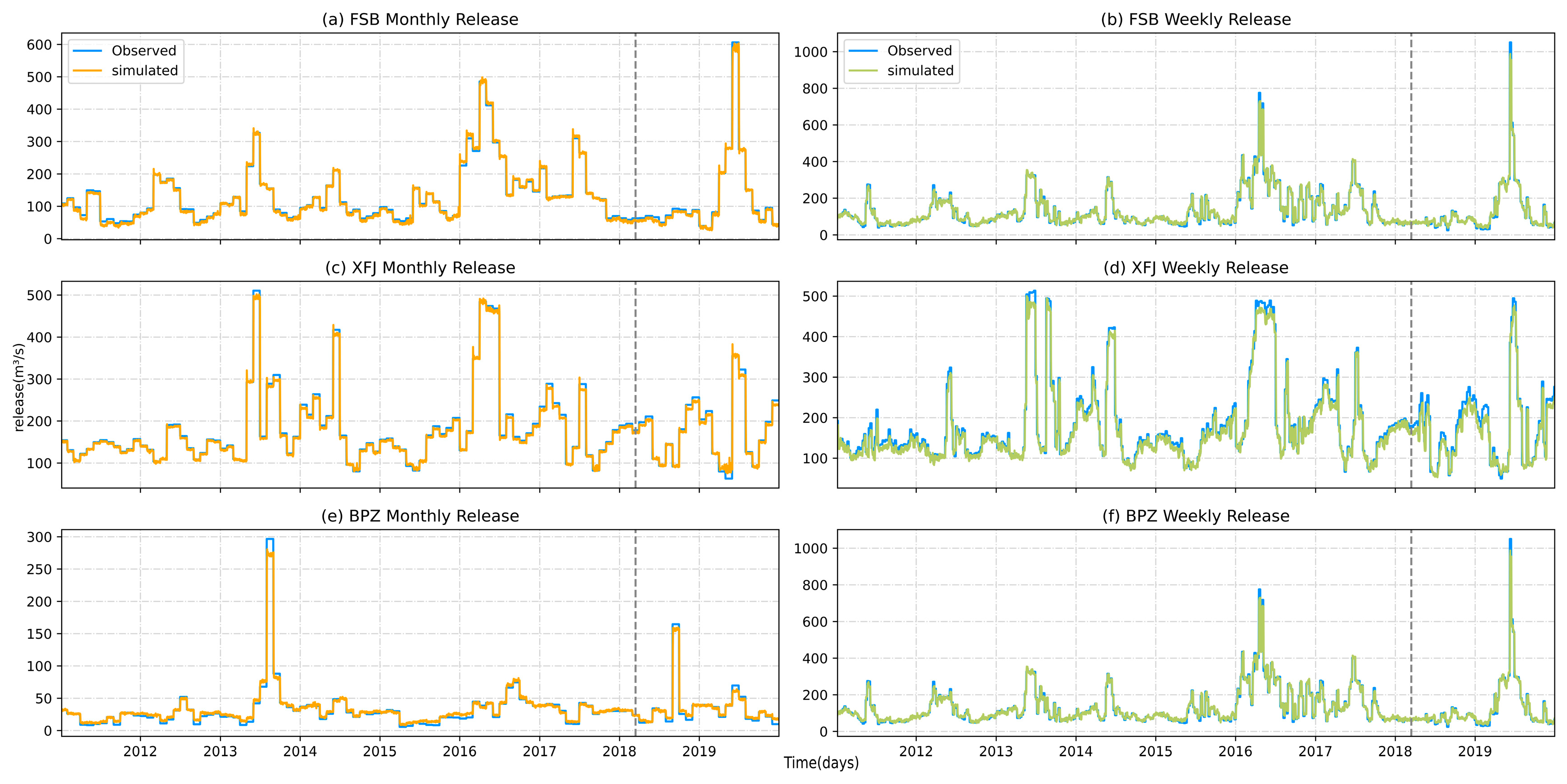
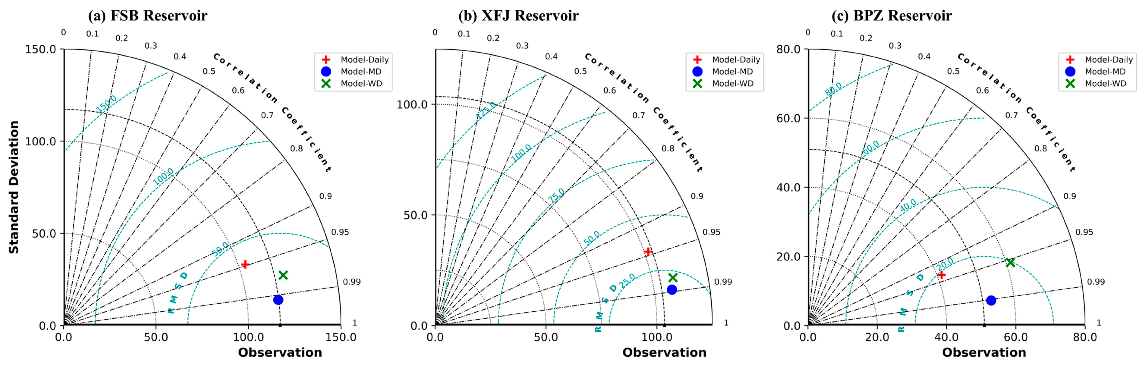
4.2. Simulation of Reservoir Operational Behavior Across Time Scales
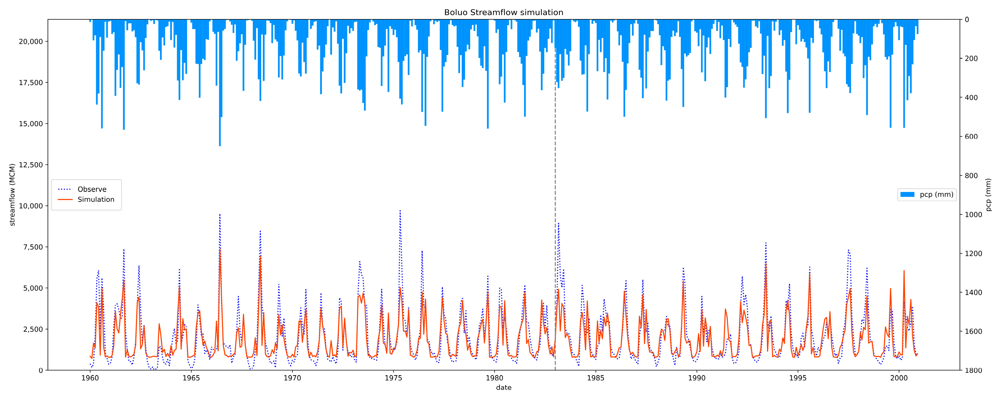
4.3. Streamflow Forecasting for Reservoir-Regulated Basins
5. Discussion
6. Conclusions
Author Contributions
Funding
Institutional Review Board Statement
Informed Consent Statement
Data Availability Statement
Acknowledgments
Conflicts of Interest
Appendix A


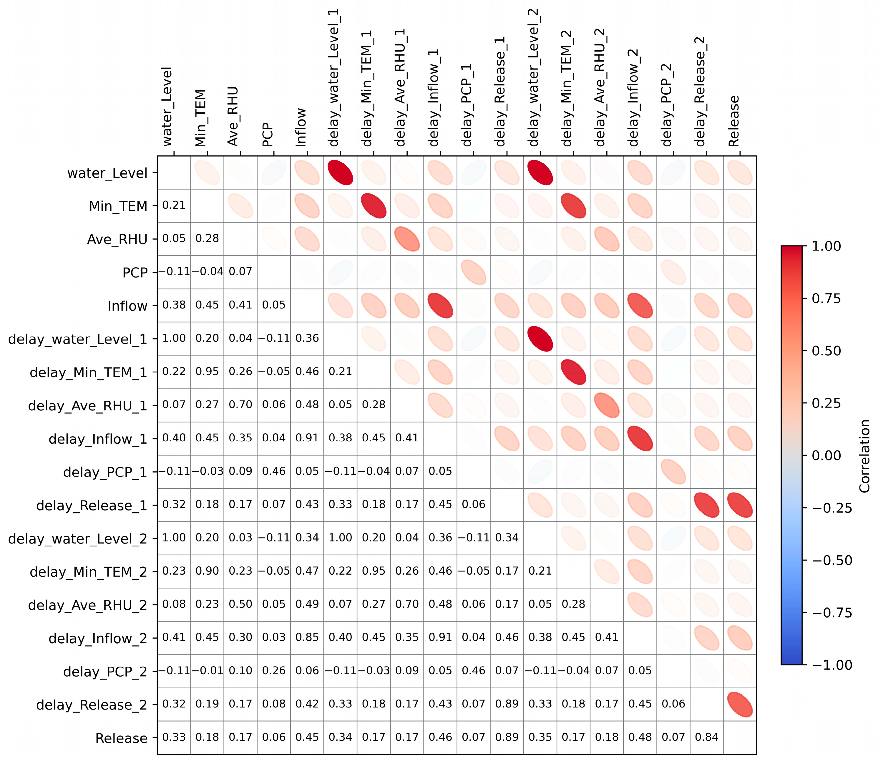
| Stations | Input Variables | Correlation |
|---|---|---|
| FSB | Water level (t), Water level (t − 1), Water level (t − 2) | 0.33–0.35 |
| Min_T (t), Min_T (t − 1), Min_T (t − 2) | 0.17–0.18 | |
| Ave_RHU (t), Ave_RHU (t − 1), Ave_RHU (t − 2) | 0.17–0.18 | |
| PCP (t), PCP (t − 1), PCP (t − 2) | 0.06–0.07 | |
| Inflow (t), Inflow (t − 1), Inflow (t − 2) | 0.45–0.48 | |
| Release (t − 1), Release (t − 2) | 0.84–0.89 | |
| XFJ | Water level (t), Water level (t − 1), Water level (t − 2) | 0.21–0.23 |
| Max_T (t), Max_T (t − 1), Max_T (t − 2) | −0.13– (−0.12) | |
| PCP (t), PCP (t − 1), PCP (t − 2) | −0.02– (−0.04) | |
| Inflow (t), Inflow (t − 1), Inflow (t − 2) | −0.01 | |
| Release (t − 1), Release (t − 2) | 0.83–0.87 | |
| BPZ | Water level (t), Water level (t − 1), Water level (t − 2) | 0.46–0.48 |
| Max_T (t), Max_T (t − 1), Max_T (t − 2) | −0.05 | |
| Ave_Wind (t), Ave_Wind (t − 1), Ave_Wind (t − 2) | 0.01–0.02 | |
| PCP (t), PCP (t − 1), PCP (t − 2) | −0.03 | |
| Inflow (t), Inflow (t − 1), Inflow (t − 2) | 0.19–0.21 | |
| Release (t − 1), Release (t − 2) | 0.91–0.95 |
| Model | Station | Number of Hidden Layers | Number of Hidden Size | Batch Size | Epochs | Learning Rate | Dropout Rate |
|---|---|---|---|---|---|---|---|
| Daily release | FSB | 2 | 196 | 100 | 56 | 0.015 | 0.001 |
| XFJ | 2 | 40 | 111 | 88 | 0.003 | 0.04 | |
| BPZ | 2 | 127 | 125 | 100 | 0.00036 | 0.056 | |
| MDF | FSB | 2 | 77 | 128 | 64 | 0.0015 | 0.001 |
| XFJ | 2 | 33 | 49 | 95 | 0.0048 | 0.027 | |
| BPZ | 2 | 31 | 46 | 95 | 0.0009 | 0.0086 | |
| WDF | FSB | 2 | 40 | 91 | 36 | 0.0022 | 0.0155 |
| XFJ | 2 | 125 | 98 | 39 | 0.00137 | 0 | |
| BPZ | 2 | 154 | 57 | 180 | 0.0002 | 0.02 |
References
- Robertson, D.E.; Shrestha, D.L.; Wang, Q.J. Post-Processing Rainfall Forecasts from Numerical Weather Prediction Models for Short-Term Streamflow Forecasting. Hydrol. Earth Syst. Sci. 2013, 17, 3587–3603. [Google Scholar] [CrossRef]
- Sadler, J.M.; Appling, A.P.; Read, J.S.; Oliver, S.K.; Jia, X.; Zwart, J.A.; Kumar, V. Multi-Task Deep Learning of Daily Streamflow and Water Temperature. Water Resour. Res. 2022, 58, e2021WR030138. [Google Scholar] [CrossRef]
- Feng, Z.; Luo, T.; Niu, W.; Yang, T.; Wang, W. A LSTM-Based Approximate Dynamic Programming Method for Hydropower Reservoir Operation Optimization. J. Hydrol. 2023, 625, 130018. [Google Scholar] [CrossRef]
- Boulange, J.; Hanasaki, N.; Yamazaki, D.; Pokhrel, Y. Role of Dams in Reducing Global Flood Exposure under Climate Change. Nat. Commun. 2021, 12, 417. [Google Scholar] [CrossRef]
- Döll, P.; Fiedler, K.; Zhang, J. Global-Scale Analysis of River Flow Alterations Due to Water Withdrawals and Reservoirs. Hydrol. Earth Syst. Sci. 2009, 13, 2413–2432. [Google Scholar] [CrossRef]
- Wang, G.; Xia, J. Improvement of SWAT2000 Modelling to Assess the Impact of Dams and Sluices on Streamflow in the Huai River Basin of China. Hydrol. Process. 2010, 24, 1455–1471. [Google Scholar] [CrossRef]
- Delaney, C.J.; Hartman, R.K.; Mendoza, J.; Dettinger, M.; Monache, L.D.; Jasperse, J.; Ralph, F.M.; Talbot, C.; Brown, J.; Reynolds, D.; et al. Forecast Informed Reservoir Operations Using Ensemble Streamflow Predictions for a Multipurpose Reservoir in Northern California. Water Resour. Res. 2010, 56, e2019WR026604. [Google Scholar] [CrossRef]
- Nayak, M.A.; Herman, J.D.; Steinschneider, S. Balancing Flood Risk and Water Supply in California: Policy Search Integrating Short-Term Forecast Ensembles with Conjunctive Use. Water Resour. Res. 2018, 54, 7557–7576. [Google Scholar] [CrossRef]
- Wang, M.; Rezaie-Balf, M.; Naganna, S.R.; Yaseen, Z.M. Sourcing CHIRPS Precipitation Data for Streamflow Forecasting Using Intrinsic Time-Scale Decomposition Based Machine Learning Models. Hydrol. Sci. J. 2021, 66, 1437–1456. [Google Scholar] [CrossRef]
- Kumar, A.; Ramsankaran, R.; Brocca, L.; Muñoz-Arriola, F. A Simple Machine Learning Approach to Model Real-Time Streamflow Using Satellite Inputs: Demonstration in a Data Scarce Catchment. J. Hydrol. 2021, 595, 126046. [Google Scholar] [CrossRef]
- Masrur Ahmed, A.A.; Deo, R.C.; Feng, Q.; Ghahramani, A.; Raj, N.; Yin, Z.; Yang, L. Deep Learning Hybrid Model with Boruta-Random Forest Optimiser Algorithm for Streamflow Forecasting with Climate Mode Indices, Rainfall, and Periodicity. J. Hydrol. 2021, 599, 126350. [Google Scholar] [CrossRef]
- Yilmaz, K.K.; Gupta, H.V.; Wagener, T. A Process-Based Diagnostic Approach to Model Evaluation: Application to the NWS Distributed Hydrologic Model. Water Resour. Res. 2008, 44, W09417. [Google Scholar] [CrossRef]
- Qian, L.; Hu, W.; Zhao, Y.; Hong, M.; Fan, L. A Coupled Model of Nonlinear Dynamical System and Deep Learning for Multi-Step Ahead Daily Runoff Prediction for Data Scarce Regions. J. Hydrol. 2025, 653, 132640. [Google Scholar] [CrossRef]
- Yokoo, K.; Ishida, K.; Ercan, A.; Tu, T.; Nagasato, T.; Kiyama, M.; Amagasaki, M. Capabilities of Deep Learning Models on Learning Physical Relationships: Case of Rainfall-Runoff Modeling with LSTM. Sci. Total Environ. 2022, 802, 149876. [Google Scholar] [CrossRef]
- Zhou, R.; Zhang, Y. Linear and Nonlinear Ensemble Deep Learning Models for Karst Spring Discharge Forecasting. J. Hydrol. 2023, 627, 130394. [Google Scholar] [CrossRef]
- Zhao, Y.; Dong, N.; Li, Z.; Zhang, W.; Yang, M.; Wang, H. Future Precipitation, Hydrology and Hydropower Generation in the Yalong River Basin: Projections and Analysis. J. Hydrol. 2021, 602, 126738. [Google Scholar] [CrossRef]
- Bhatta, B.; Shrestha, S.; Shrestha, P.K.; Talchabhadel, R. Evaluation and Application of a SWAT Model to Assess the Climate Change Impact on the Hydrology of the Himalayan River Basin. CATENA 2019, 181, 104082. [Google Scholar] [CrossRef]
- Palmer, M.; Ruhi, A. Linkages between Flow Regime, Biota, and Ecosystem Processes: Implications for River Restoration. Science 2019, 365, eaaw2087. [Google Scholar] [CrossRef]
- Coerver, H.M.; Rutten, M.M.; van de Giesen, N.C. Deduction of Reservoir Operating Rules for Application in Global Hydrological Models. Hydrol. Earth Syst. Sci. 2018, 22, 831–851. [Google Scholar] [CrossRef]
- Shin, S.; Pokhrel, Y.; Miguez-Macho, G. High-Resolution Modeling of Reservoir Release and Storage Dynamics at the Con-tinental Scale. Water Resour. Res. 2019, 55, 787–810. [Google Scholar] [CrossRef]
- Yang, S.; Yang, D.; Chen, J.; Zhao, B. Real-Time Reservoir Operation Using Recurrent Neural Networks and Inflow Forecast from a Distributed Hydrological Model. J. Hydrol. 2019, 579, 124229. [Google Scholar] [CrossRef]
- Shrestha, J.P.; Pahlow, M.; Cochrane, T.A. Development of a SWAT Hydropower Operation Routine and Its Application to Assessing Hydrological Alterations in the Mekong. Water 2020, 12, 2193. [Google Scholar] [CrossRef]
- Wang, Z.; He, Y.; Li, W.; Chen, X.; Yang, P.; Bai, X. A Generalized Reservoir Module for SWAT Applications in Watersheds Regulated by Reservoirs. J. Hydrol. 2023, 616, 128770. [Google Scholar] [CrossRef]
- Blöschl, G.; Bierkens, M.F.P.; Chambel, A.; Cudennec, C.; Destouni, G.; Fiori, A.; Kirchner, J.W.; McDonnell, J.J.; Savenije, H.H.G.; Sivapalan, M.; et al. Twenty-Three Unsolved Problems in Hydrology (UPH)—A Community Perspective. Hydrol. Sci. J. 2019, 64, 1141–1158. [Google Scholar] [CrossRef]
- Wang, N.; Zhang, D.; Chang, H.; Li, H. Deep Learning of Subsurface Flow via Theory-Guided Neural Network. J. Hydrol. 2020, 584, 124700. [Google Scholar] [CrossRef]
- Quinn, J.D.; Reed, P.M.; Giuliani, M.; Castelletti, A. What Is Controlling Our Control Rules? Opening the Black Box of Mul-tireservoir Operating Policies Using Time-Varying Sensitivity Analysis. Water Resour. Res. 2019, 55, 5962–5984. [Google Scholar] [CrossRef]
- Lundberg, S.M.; Lee, S.-I. A Unified Approach to Interpreting Model Predictions. In Advances in Neural Information Processing Systems; Guyon, I., Von Luxburg, U., Bengio, S., Wallach, H., Fergus, R., Vishwanathan, S., Garnett, R., Eds.; Curran Associates, Inc.: New York, NY, USA, 2017; Volume 30. [Google Scholar]
- Mazrooei, A.; Sankarasubramanian, A.; Wood, A.W. Potential in Improving Monthly Streamflow Forecasting through Var-iational Assimilation of Observed Streamflow. J. Hydrol. 2021, 600, 126559. [Google Scholar] [CrossRef]
- Sushanth, K.; Mishra, A.; Mukhopadhyay, P.; Singh, R. Real-Time Streamflow Forecasting in a Reservoir-Regulated River Basin Using Explainable Machine Learning and Conceptual Reservoir Module. Sci. Total Environ. 2023, 861, 160680. [Google Scholar] [CrossRef]
- Oliveira, R.; Loucks, D.P. Operating Rules for Multireservoir Systems. Water Resour. Res. 1997, 33, 839–852. [Google Scholar] [CrossRef]
- Longyang, Q.; Zeng, R. A Hierarchical Temporal Scale Framework for Data-Driven Reservoir Release Modeling. Water Resour. Res. 2023, 59, e2022WR033922. [Google Scholar] [CrossRef]
- Hochreiter, S.; Schmidhuber, J. Long Short-Term Memory. Neural Comput. 1997, 9, 1735–1780. [Google Scholar] [CrossRef]
- Hashemi, R.; Brigode, P.; Garambois, P.-A.; Javelle, P. How Can We Benefit from Regime Information to Make More Effective Use of Long Short-Term Memory (LSTM) Runoff Models? Hydrol. Earth Syst. Sci. 2022, 26, 5793–5816. [Google Scholar] [CrossRef]
- Yang, T.; Zhang, L.; Kim, T.; Hong, Y.; Zhang, D.; Peng, Q. A Large-Scale Comparison of Artificial Intelligence and Data Mining (AI&DM) Techniques in Simulating Reservoir Releases over the Upper Colorado Region. J. Hydrol. 2021, 602, 126723. [Google Scholar] [CrossRef]
- Shen, C. A Transdisciplinary Review of Deep Learning Research and Its Relevance for Water Resources Scientists. Water Resour. Res. 2018, 54, 8558–8593. [Google Scholar] [CrossRef]
- Feng, D.; Fang, K.; Shen, C. Enhancing Streamflow Forecast and Extracting Insights Using Long-Short Term Memory Networks with Data Integration at Continental Scales. Water Resour. Res. 2020, 56, e2019WR026793. [Google Scholar] [CrossRef]
- Akiba, T.; Sano, S.; Yanase, T.; Ohta, T.; Koyama, M. Optuna: A Next-Generation Hyperparameter Optimization Framework. In Proceedings of the 25th ACM SIGKDD International Conference on Knowledge Discovery & Data Mining, Anchorage, AK, USA, 4–8 August 2019; Association for Computing Machinery: New York, NY, USA, 2019; pp. 2623–2631. [Google Scholar]
- Fu, B.; Liang, Y.; Lao, Z.; Sun, X.; Li, S.; He, H.; Sun, W.; Fan, D. Quantifying Scattering Characteristics of Mangrove Species from Optuna-Based Optimal Machine Learning Classification Using Multi-Scale Feature Selection and SAR Image Time Series. Int. J. Appl. Earth Obs. Geoinf. 2023, 122, 103446. [Google Scholar] [CrossRef]
- Lin, N.; Zhang, D.; Feng, S.; Ding, K.; Tan, L.; Wang, B.; Chen, T.; Li, W.; Dai, X.; Pan, J.; et al. Rapid Landslide Extraction from High-Resolution Remote Sensing Images Using SHAP-OPT-XGBoost. Remote Sens. 2023, 15, 3901. [Google Scholar] [CrossRef]
- Zou, Y.; Wang, J.; Lei, P.; Li, Y. A Novel Multi-Step Ahead Forecasting Model for Flood Based on Time Residual LSTM. J. Hydrol. 2023, 620, 129521. [Google Scholar] [CrossRef]
- Li, D.; Chen, Y.; Lyu, L.; Cai, X. Uncovering Historical Reservoir Operation Rules and Patterns: Insights From 452 Large Reservoirs in the Contiguous United States. Water Resour. Res. 2024, 60, e2023WR036686. [Google Scholar] [CrossRef]
- Ding, Z.; Fang, G.; Wen, X.; Tan, Q.; Huang, X.; Lei, X.; Tian, Y.; Quan, J. A Novel Operation Chart for Cascade Hydropower System to Alleviate Ecological Degradation in Hydrological Extremes. Ecol. Model. 2018, 384, 10–22. [Google Scholar] [CrossRef]
- Zhang, J.; Yan, H. A Long Short-Term Components Neural Network Model with Data Augmentation for Daily Runoff Forecasting. J. Hydrol. 2023, 617, 128853. [Google Scholar] [CrossRef]
- He, S.; Niu, G.; Sang, X.; Sun, X.; Yin, J.; Chen, H. Machine Learning Framework with Feature Importance Interpretation for Discharge Estimation: A Case Study in Huitanggou Sluice Hydrological Station, China. Water 2023, 15, 1923. [Google Scholar] [CrossRef]
- Shadmani, M.; Marofi, S.; Roknian, M. Trend Analysis in Reference Evapotranspiration Using Mann-Kendall and Spearman’s Rho Tests in Arid Regions of Iran. Water Resour. Manag. 2012, 26, 211–224. [Google Scholar] [CrossRef]
- Luo, X.; Yuan, X.; Zhu, S.; Xu, Z.; Meng, L.; Peng, J. A Hybrid Support Vector Regression Framework for Streamflow Forecast. J. Hydrol. 2019, 568, 184–193. [Google Scholar] [CrossRef]
- Sang, X.; Wang, H.; Wang, J.; Zhao, Y.; Zhou, Z. Water Resources Comprehensive Allocation and Simulation Model (WAS), part I. Theory and development. J. Hydraul. Eng. 2018, 49, 1451–1459. (In Chinese) [Google Scholar] [CrossRef]
- Sang, X.; Zhao, Y.; Zhai, Z.; Chang, H. Water resources comprehensive allocation and simulation model (WAS), part II. Application. J. Hydraul. Eng. 2019, 50, 201–208. (In Chinese) [Google Scholar] [CrossRef]
- Zheng, Y.; Sang, X.; Li, Z.; Zhang, S.; Chang, J. Ecological Services Value of ‘Natural-Artificial’ Water Cycle: Valuation Method and Its Application in the Yangtze River Basin of China. Ecol. Indic. 2024, 158, 111324. [Google Scholar] [CrossRef]
- Yan, Z.; Zhou, Z.; Sang, X.; Wang, H. Water Replenishment for Ecological Flow with an Improved Water Resources Allocation Model. Sci. Total Environ. 2018, 643, 1152–1165. [Google Scholar] [CrossRef]
- Chang, H.; Sang, X.; He, G.; Wang, Q.; Chang, J.; Liu, R.; Li, H.; Zhao, Y. A Socio-Hydrological Unit Division and Confluence Relationship Generation Method for Human–Water Systems. Water 2022, 14, 2074. [Google Scholar] [CrossRef]
- Zheng, Y.; Sang, X.; Liu, Z.; Zhang, S.; Liu, P. Water Allocation Management Under Scarcity: A Bankruptcy Approach. Water Resour. Manag. 2022, 36, 2891–2912. [Google Scholar] [CrossRef]
- Xu, W.; Chen, J.; Corzo, G.; Xu, C.-Y.; Zhang, X.J.; Xiong, L.; Liu, D.; Xia, J. Coupling Deep Learning and Physically Based Hydrological Models for Monthly Streamflow Predictions. Water Resour. Res. 2024, 60, e2023WR035618. [Google Scholar] [CrossRef]
- Hao, N.; Sun, P.; He, W.; Yang, L.; Qiu, Y.; Chen, Y.; Zhao, W. Water Resources Allocation in the Tingjiang River Basin: Construction of an Interval-Fuzzy Two-Stage Chance-Constraints Model and Its Assessment through Pearson Correlation. Water 2022, 14, 2928. [Google Scholar] [CrossRef]
- Wu, J.; Wang, G.; Chen, X.; Chen, X. Evolutionary of Hydrological Drought and its Impact on Large Reservoir Regulation—A Case Study of the Dongjiang River Basin with Multiple Reservoir Regulation. Water Resour. Prot. 2024, 40, 52–60. Available online: http://kns.cnki.net/kcms/detail/32.1356.TV.20240308.1457.004.html (accessed on 24 April 2025). (In Chinese).
- Wang, T.; Tu, X.; Singh, V.P.; Chen, X.; Lin, K.; Zhou, Z.; Tan, Y. Assessment of Future Socioeconomic Drought Based on CMIP6: Evolution, Driving Factors and Propagation. J. Hydrol. 2023, 617, 129009. [Google Scholar] [CrossRef]
- Zhou, Z.; Tu, X.; Wang, T.; Singh, V.P.; Chen, X.; Lin, K. Bivariate Socioeconomic Drought Assessment Based on a Hybrid Framework and Impact of Human Activities. J. Clean. Prod. 2023, 409, 137150. [Google Scholar] [CrossRef]
- Wang, T.; Tu, X.; Singh, V.P.; Chen, X.; Lin, K.; Lai, R.; Zhou, Z. Socioeconomic Drought Analysis by Standardized Water Supply and Demand Index under Changing Environment. J. Clean. Prod. 2022, 347, 131248. [Google Scholar] [CrossRef]
- Wang, J.; Wang, X.; Khu, S.T. A Decomposition-Based Multi-Model and Multi-Parameter Ensemble Forecast Framework for Monthly Streamflow Forecasting. J. Hydrol. 2023, 618, 129083. [Google Scholar] [CrossRef]
- Gao, S.; Huang, Y.; Zhang, S.; Han, J.; Wang, G.; Zhang, M.; Lin, Q. Short-Term Runoff Prediction with GRU and LSTM Networks without Requiring Time Step Optimization during Sample Generation. J. Hydrol. 2020, 589, 125188. [Google Scholar] [CrossRef]
- Arheimer, B.; Donnelly, C.; Lindström, G. Regulation of Snow-Fed Rivers Affects Flow Regimes More than Climate Change. Nat. Commun. 2017, 8, 62. [Google Scholar] [CrossRef]
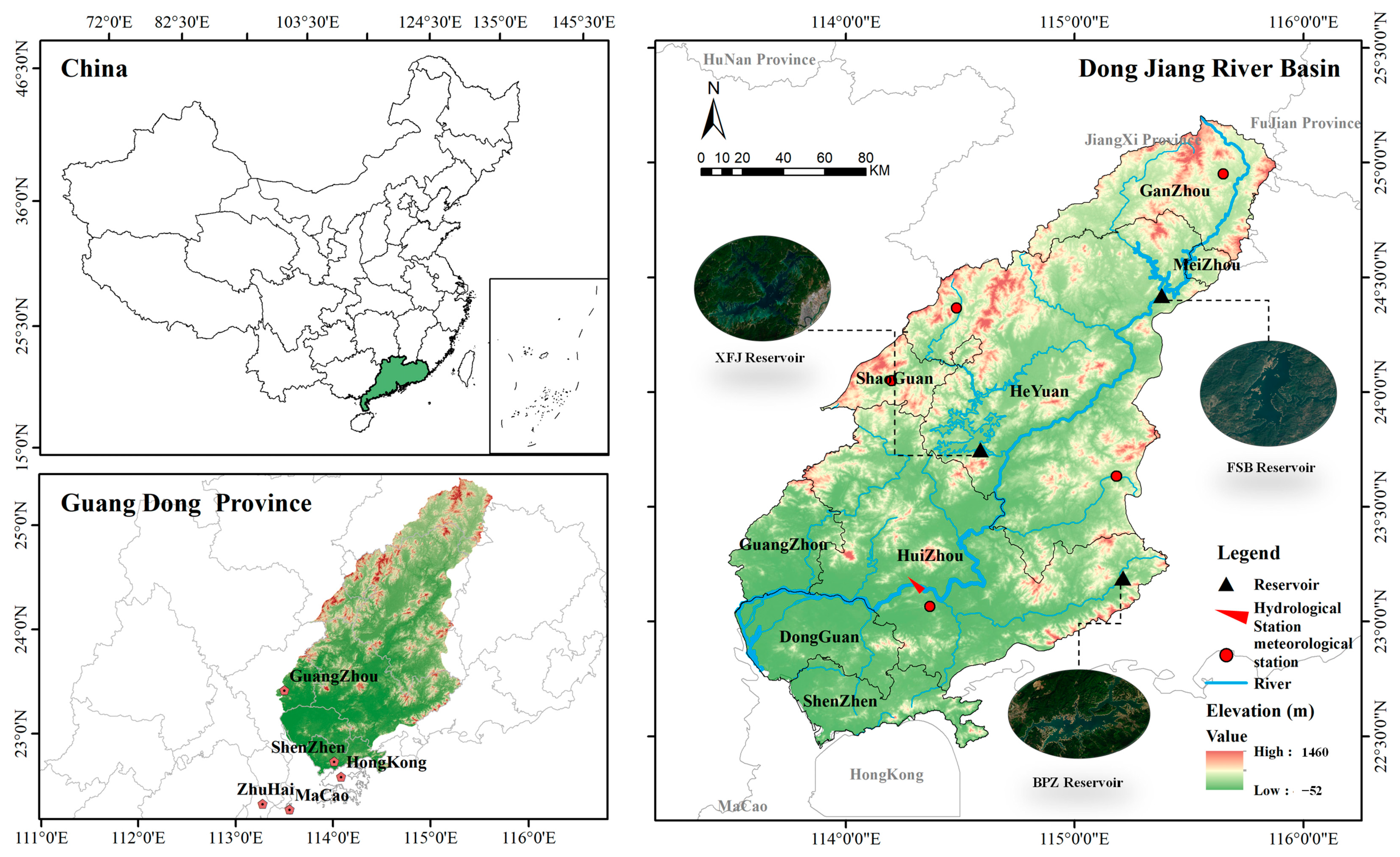


| Reservoir | Catchment Area/km2 | Capacity/km3 | Operation Year | Data Period |
|---|---|---|---|---|
| FSB | 5150 | 1.93 | 1983 | 2011–2019 |
| XFJ | 5734 | 13.9 | 1960 | 2011–2019 |
| BPZ | 856 | 1.22 | 1987 | 2011–2019 |
| Period | Performance Index | Reservoir | |||||
|---|---|---|---|---|---|---|---|
| FSB | XFJ | BPZ | |||||
| Monthly | Weekly | Monthly | Weekly | Monthly | Weekly | ||
| Training | NSE | 0.97 | 0.94 | 0.97 | 0.95 | 0.95 | 0.82 |
| R | 0.99 | 0.97 | 0.98 | 0.98 | 0.98 | 0.9 | |
| MAE (m3/s) | 10.81 | 11.69 | 5.65 | 10.4 | 2.7 | 6.23 | |
| RMSE (m3/s) | 15.13 | 23.8 | 16.03 | 21 | 7.16 | 20.65 | |
| Testing | NSE | 0.95 | 0.93 | 0.95 | 0.93 | 0.92 | 0.83 |
| R | 0.99 | 0.96 | 0.97 | 0.96 | 0.96 | 0.91 | |
| MAE (m3/s) | 16.72 | 13.08 | 7.42 | 13.99 | 3.34 | 6.96 | |
| RMSE (m3/s) | 27.06 | 37.91 | 17.6 | 25.46 | 9.28 | 17.07 | |
| Period | Performance Index | Reservoir | |||||
|---|---|---|---|---|---|---|---|
| FSB | XFJ | BPZ | |||||
| Monthly Benchmark | Weekly Benchmark | Monthly Benchmark | Weekly Benchmark | Monthly Benchmark | Weekly Benchmark | ||
| Training | NSE | 0.26 | 0.23 | 0.15 | 0.16 | 0.15 | 0.39 |
| R | 0.51 | 0.48 | 0.38 | 0.4 | 0.39 | 0.39 | |
| MAE (m3/s) | 50 | 56.87 | 57.45 | 62.98 | 15.12 | 6.23 | |
| RMSE (m3/s) | 71 | 83.89 | 82.67 | 90.52 | 30.26 | 20.65 | |
| Testing | NSE | 0.39 | 0.41 | 0.41 | 0.37 | 0.42 | 0.67 |
| R | 0.63 | 0.64 | 0.64 | 0.61 | 0.65 | 0.67 | |
| MAE (m3/s) | 60.55 | 64.94 | 40.18 | 48.59 | 13.44 | 6.96 | |
| RMSE (m3/s) | 97.81 | 13.07 | 59.61 | 73.86 | 24.32 | 17.07 | |
| Res_Name | Performance Metrics | Model | ||
|---|---|---|---|---|
| MD | WD | Daily | ||
| FSB | NSE | 0.98 | 0.94 | 0.92 |
| XFJ | 0.97 | 0.93 | 0.83 | |
| BPZ | 0.96 | 0.85 | 0.78 | |
| FSB | RMSE | 20.7 | 37.5 | 43.4 |
| XFJ | 18.7 | 26.7 | 40.2 | |
| BPZ | 8.9 | 17.1 | 20.9 | |
| FSB | MAE | 5.5 | 12.7 | 22.4 |
| XFJ | 10.5 | 16.7 | 25.5 | |
| BPZ | 3.5 | 5.8 | 8.18 | |
| FSB | R | 0.99 | 0.95 | 0.93 |
| XFJ | 0.99 | 0.98 | 0.94 | |
| BPZ | 0.99 | 0.95 | 0.93 | |
Disclaimer/Publisher’s Note: The statements, opinions and data contained in all publications are solely those of the individual author(s) and contributor(s) and not of MDPI and/or the editor(s). MDPI and/or the editor(s) disclaim responsibility for any injury to people or property resulting from any ideas, methods, instructions or products referred to in the content. |
© 2025 by the authors. Licensee MDPI, Basel, Switzerland. This article is an open access article distributed under the terms and conditions of the Creative Commons Attribution (CC BY) license (https://creativecommons.org/licenses/by/4.0/).
Share and Cite
Chang, J.; Sang, X.; Qu, J.; Jia, Y.; Wang, L.; Ding, H. Hierarchical Temporal-Scale Framework for Real-Time Streamflow Prediction in Reservoir-Regulated Basins. Sustainability 2025, 17, 4046. https://doi.org/10.3390/su17094046
Chang J, Sang X, Qu J, Jia Y, Wang L, Ding H. Hierarchical Temporal-Scale Framework for Real-Time Streamflow Prediction in Reservoir-Regulated Basins. Sustainability. 2025; 17(9):4046. https://doi.org/10.3390/su17094046
Chicago/Turabian StyleChang, Jiaxuan, Xuefeng Sang, Junlin Qu, Yangwen Jia, Lin Wang, and Haokai Ding. 2025. "Hierarchical Temporal-Scale Framework for Real-Time Streamflow Prediction in Reservoir-Regulated Basins" Sustainability 17, no. 9: 4046. https://doi.org/10.3390/su17094046
APA StyleChang, J., Sang, X., Qu, J., Jia, Y., Wang, L., & Ding, H. (2025). Hierarchical Temporal-Scale Framework for Real-Time Streamflow Prediction in Reservoir-Regulated Basins. Sustainability, 17(9), 4046. https://doi.org/10.3390/su17094046