
Techno-Economic Analysis of Operating Temperature Variations in a 4th Generation District Heating Grid—A German Case Study


Abstract
:1. Introduction
1.1. Motivation
1.2. State of the Art
1.2.1. District
1.2.2. District Heating Grid
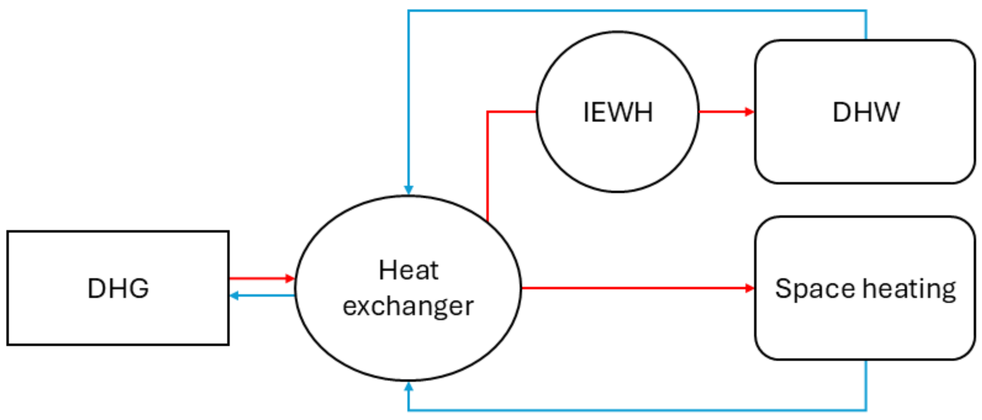
1.2.3. Domestic Hot Water Supply
1.2.4. Regulatory Framework
1.3. Research Question and Structure
2. Materials and Methods
2.1. nPro
2.1.1. First Model
2.1.2. Second Model
2.1.3. Third Model
2.2. Case Study
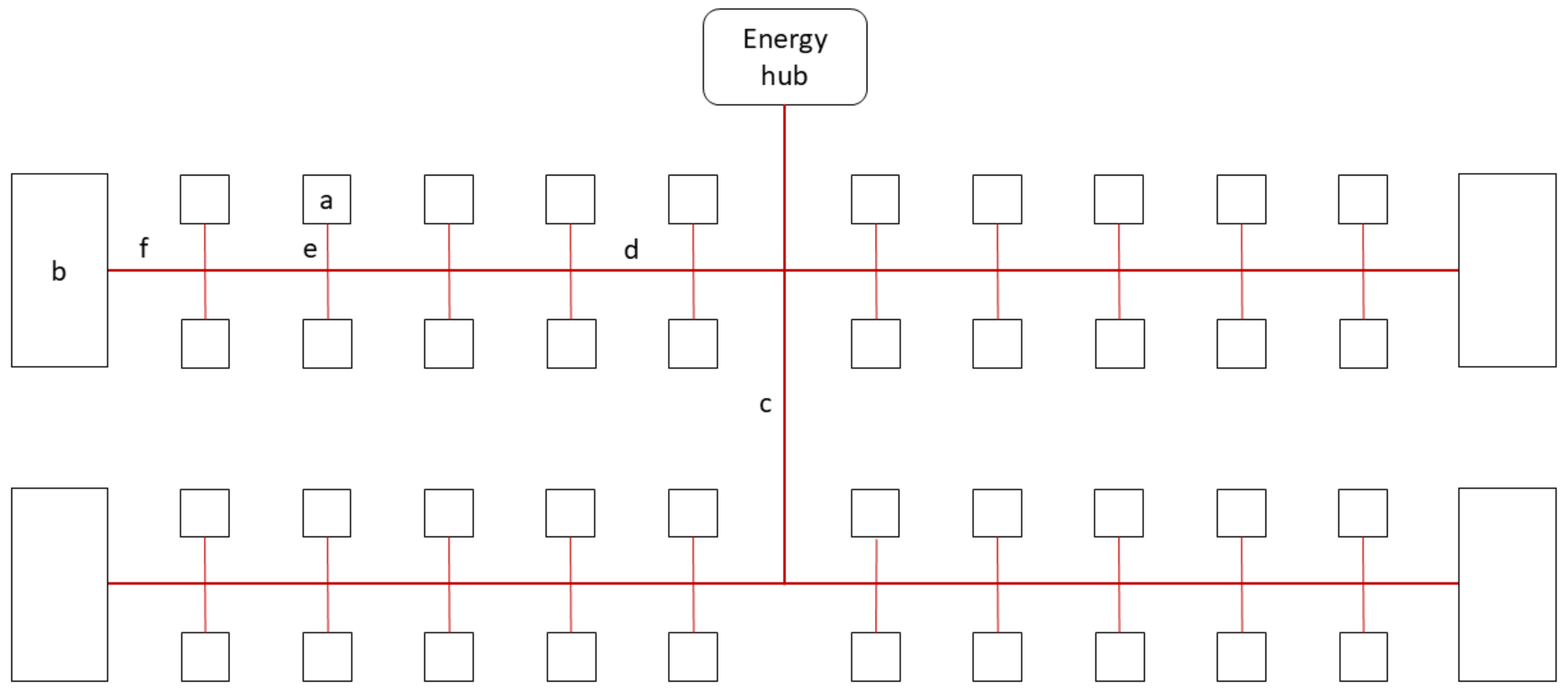
2.2.1. District
2.2.2. Space Heating and Domestic Hot Water
2.2.3. District Heating Grid
- LCOHscX is the levelized cost of heating of scenario X [EUR/MWhth];
- TscX is the DH temperature of scenario X [°C].
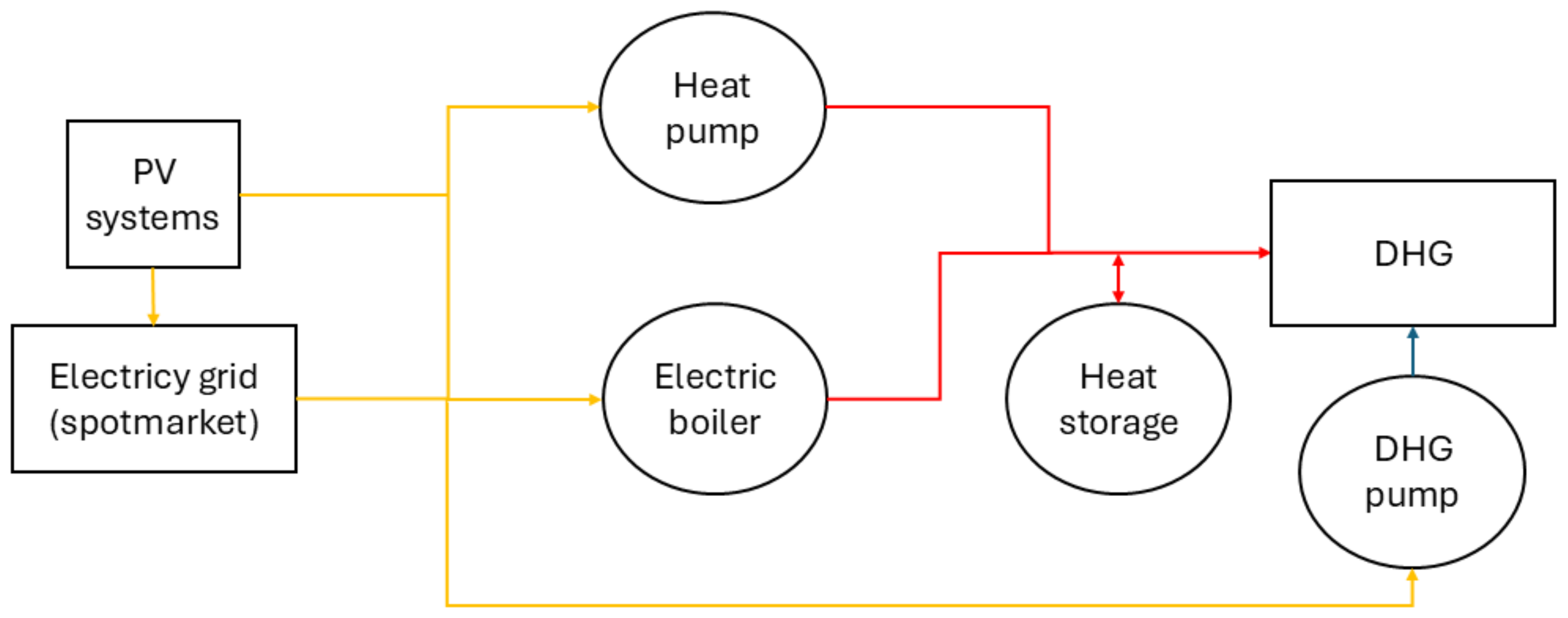
2.2.4. Energy Hub
2.3. Further Assumptions
3. Results
3.1. Techno-Economic Optimization
3.1.1. Heat Demand of the District
3.1.2. Dimensioning and Operation of the District Heating Grid
3.1.3. Design of the Energy Hub
3.2. Summary of the Energy System Sections
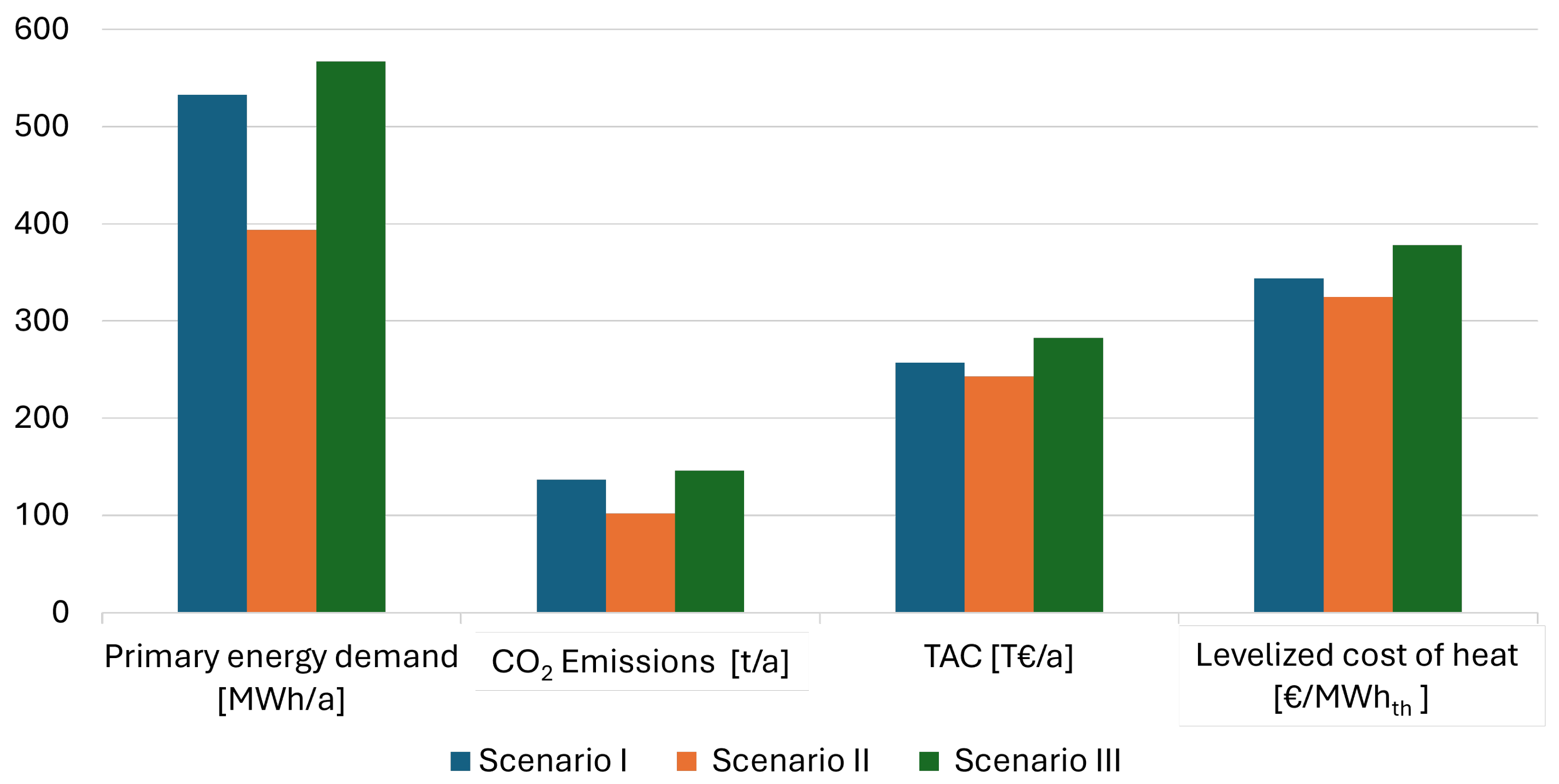
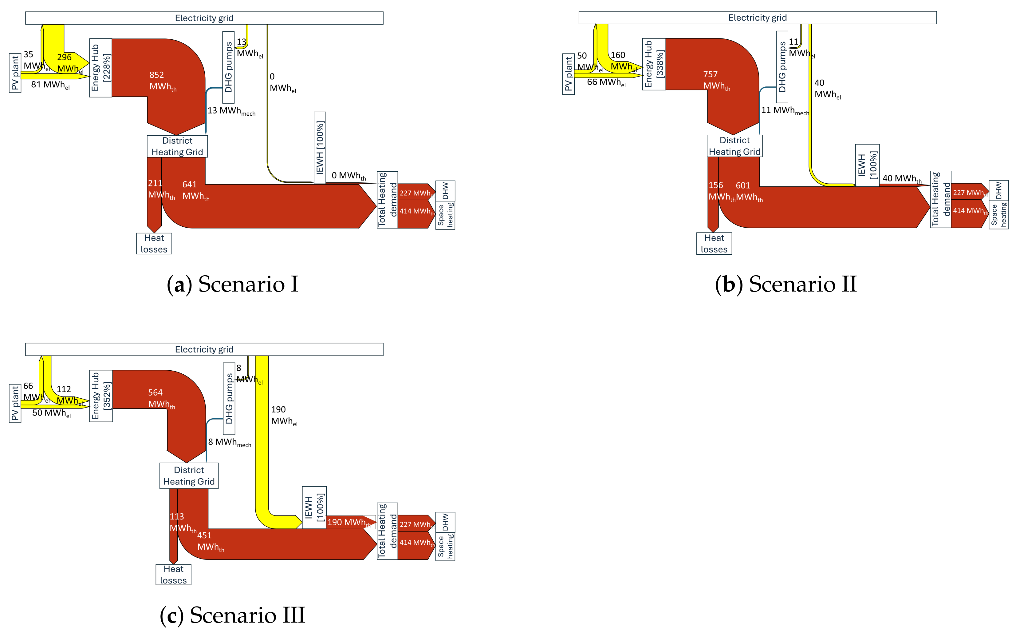
3.2.1. Primary Energy Demand and Energy Flows
3.2.2. Emissions
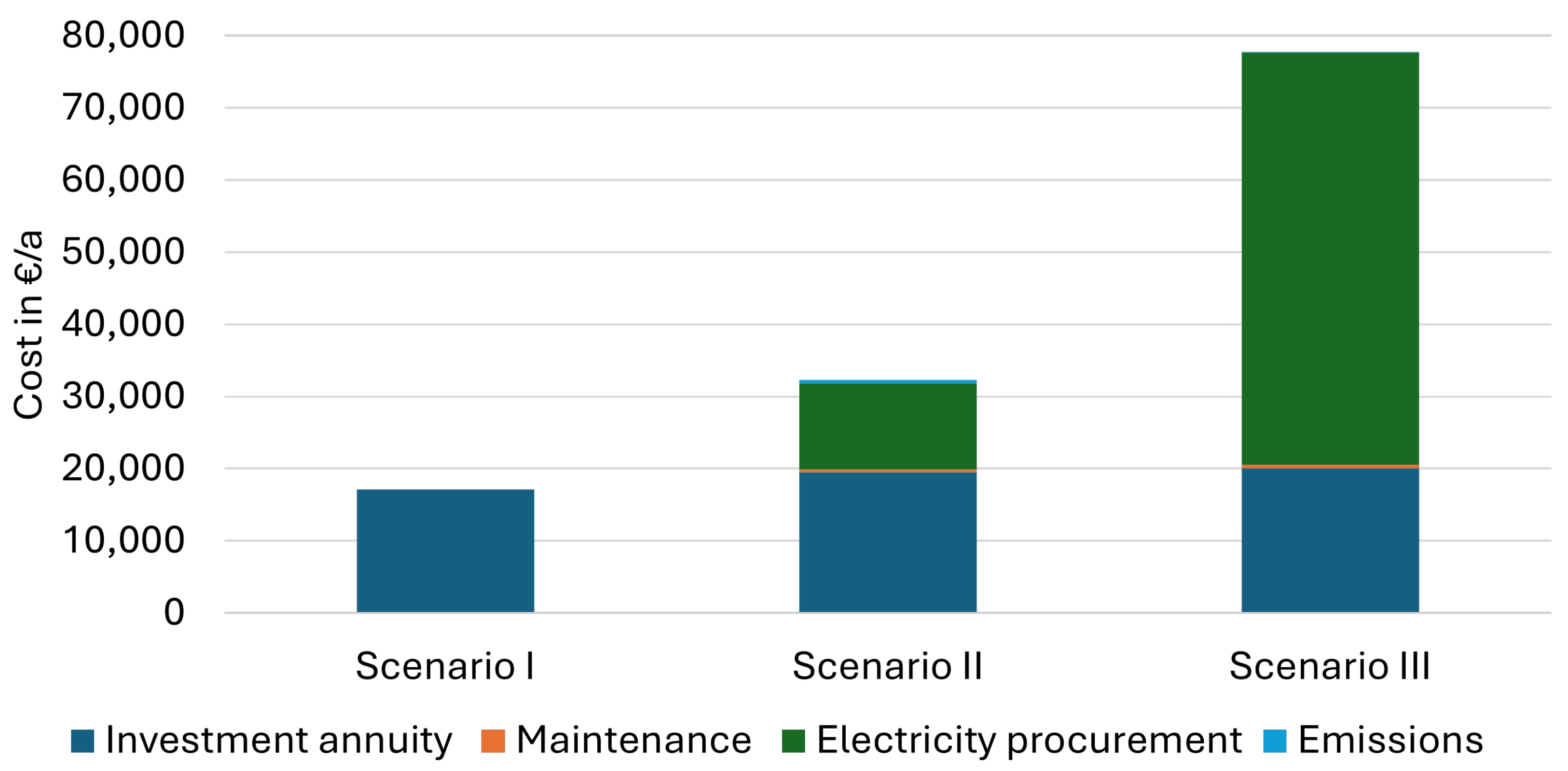
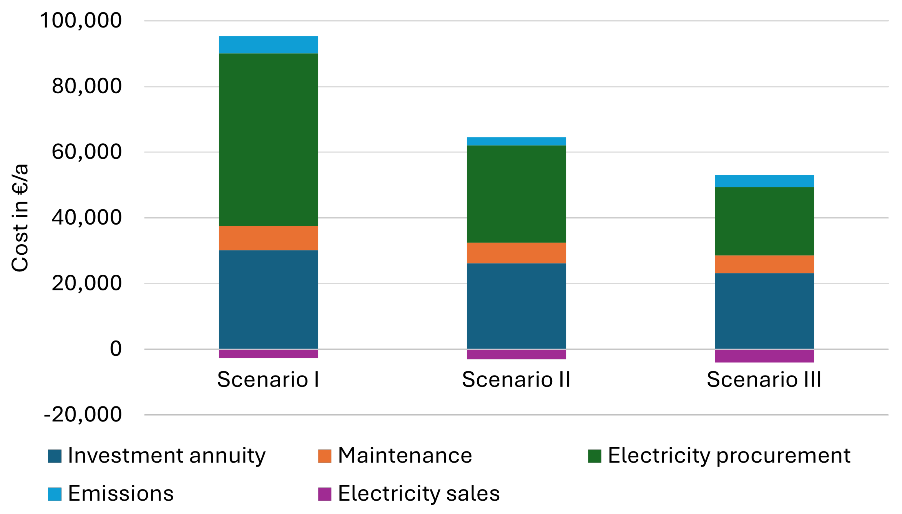
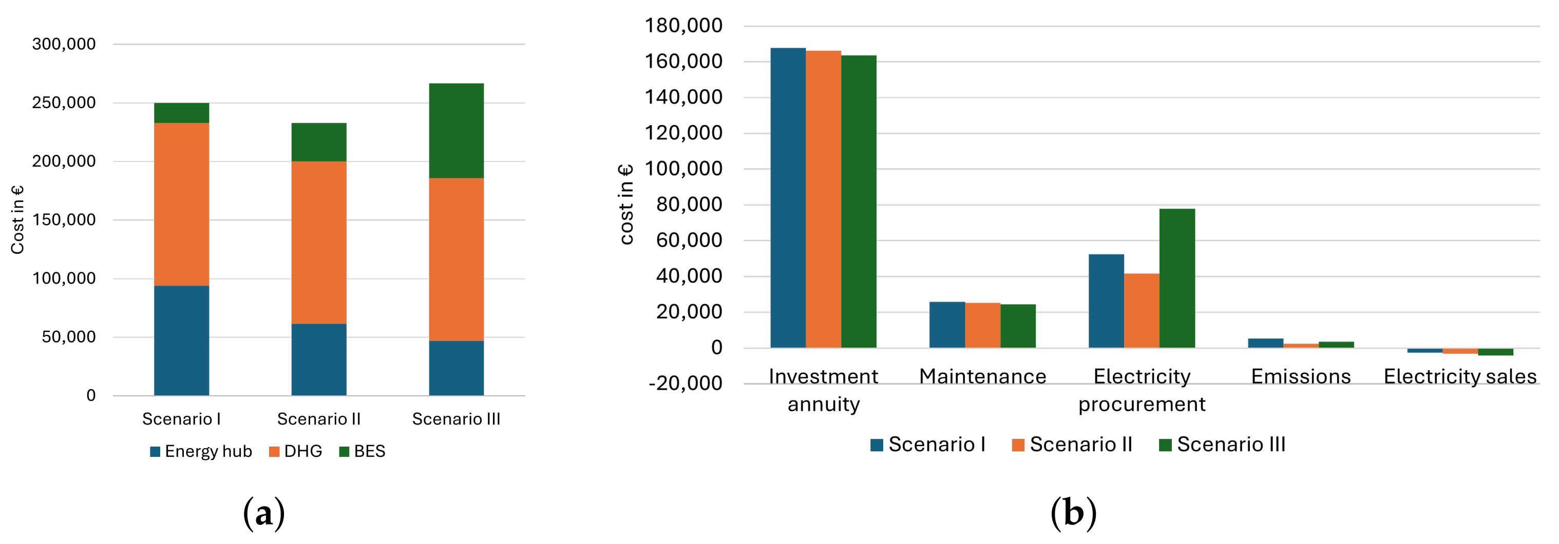
3.2.3. Costs
3.3. Positive Energy District
4. Discussion
4.1. Operating Temperature
4.2. Electrification
4.3. Cost Distribution and LCOH
4.4. Communal Heat Planning
4.5. Positive Energy District
4.6. Limitations and Further Research
5. Conclusions
Author Contributions
Funding
Data Availability Statement
Acknowledgments
Conflicts of Interest
Abbreviations and Nomenclature
| 4GDHG | 4th generation of district heating grid |
| 5GDHG | 5th generation of district heating grid |
| BCP | Building Connection Pipe |
| BEHG | German Fuel Emissions Trading Act |
| BES | Building Energy System |
| CHP | Combined Heat and Power |
| CRG | Cost Reduction Gradient |
| COP | Coefficient of Performance |
| EEG | German Renewable Energies Act |
| EEX | European Energy Exchange AG |
| EnEV | Energy Saving Ordinance |
| EnFG | German Energy Financing Act |
| EnWG | German Energy Industry Act |
| EEWärmeG | Renewable Energy Heat |
| DH | District heating |
| DHG | District heating grid |
| DHW | Domestic hot water |
| DCW | Domestic cold water |
| GEG | German Building Energy Act |
| HP | Heat Pump |
| IEWH | Instantaneous electric water heater |
| KAV | German Concession Fee Ordinance |
| KfW | Credit Institute for Reconstruction |
| KWKG | German Combined Heat and Power Act |
| LCOH | Levelized cost of heating |
| MFR | Multi-family residence |
| P2H | Power-to-Heat |
| PED | Postive Energy District |
| PV | Photovoltaics |
| RES | Renewable Energy Sources |
| SFR | Single-family residence |
| TAC | Total Annual Cost |
| StromNEV | German Electricity Grid Charges Ordinance |
| StromStG | German Electricity Tax Act |
| WPG | Heat Planning Act |
| A | Area | |
| c | cost | EUR |
| Cost Reduction Gradient | EUR/MWhth °C | |
| E | Electricity | MWhel |
| CO2 emissions | kg CO2 | |
| k | Thermal conductivity | Whth/mK |
| Levelized Cost of Heating | EUR/MWhth | |
| Price for CO2 emission certificate | EUR/t CO2 | |
| Electricity price | EUR/kWhel | |
| Peak power PV | kWp | |
| Q | Heat | MWhth |
| Space heating requirement | kWhth/m2 | |
| Heat loss per pipe section | kWhth/m | |
| T | Temperature | °C or K |
Appendix A. Calculations of the Heating Share
- QInput is the total energy inflow into the energy transfer station [kWhth];
- QDHG of the thermal energy is provided by the DHG [kWhth];
- QIEWH is the thermal supply of the IEWH for the additional heating of the DHW [kWHth].
- QOutput is the total energy outflow from the energy transfer station [kWhth];
- QDHW is the thermal energy demand required for the DHW supply [kWhth];
- QLoss is the heat losses that occur during DHW supply [kWhth].
- TDHG the temperature of the DHG [°C],
- TDCW the temperature of the DCW [°C],
- TDHW the required temperature of the DHW [°C].
Appendix B. Tables

| Technology | Specific Investment | Fixed Investment | Lifetime | Maintenance |
|---|---|---|---|---|
| Units | EUR/kWhth, EUR/m3, EUR/kWp | EUR/Building | Years | % of Investment/Year |
| DHG connection | 200 | 4000 | 40 | 0 |
| IEWH | 150 | 1000 | 25 | 1 |
| DHG | see Table A2 | - | 40 | 1 |
| Air-source HP | 500 | - | 20 | 2.5 |
| Electric boiler | 80 | - | 20 | 3 |
| Heat Storage (m3) | 500 | - | 20 | 1 |
| PV systems (kWp) | 900 | - | 20 | 1 |
| Inner Diameter | Pipe Cost | Trench Cost |
|---|---|---|
| Unit | EUR/m | EUR/m |
| DN 25 | 260 | 240 |
| DN 32 | 270 | 250 |
| DN 50 | 290 | 270 |
| DN 80 | 350 | 300 |
| Temperature of the Heat Source | Temperature of the Heat Sink | ||
|---|---|---|---|
| 35 °C | 45 °C | 55 °C | |
| −7 °C | 3.13 | 2.42 | 1.70 |
| 2 °C | 4.04 | 3.33 | 2.61 |
| 7 °C | 4.95 | 4.24 | 3.52 |
| 12 °C | 5.86 | 5.15 | 4.43 |
| Entry | Unit | Value |
|---|---|---|
| Time horizon | years | 20 |
| Interest rate | % | 5 |
| Heat transfer gradient | K | 2 |
| Day-Ahead Spotmarket | EUR/MWh | Time series |
| Operating power costs | EUR/MWh | 300 |
| Electricity emission factor | t/MWh | 0.387 |
| Electricity primary energy factor | 1.5 | |
| CO2 price | EUR/t | 45 |
| PV feed-in compensation | EUR/MWh | 74.3 |
| Scenario I | Unit | DHG Connection | IEWH |
|---|---|---|---|
| Number | 44 | - | |
| Capacity | kWth | 435 | - |
| Useful energy | MWhth | 641 | - |
| Investment | EUR | 262,932 | - |
| Annuity | EUR/a | 17,122 | - |
| Scenario I | Unit | DHG Connection | IEWH |
|---|---|---|---|
| Number | 44 | 44 | |
| Capacity | kWth | 357 | 11 |
| Useful energy | MWhth | 601 | 40 |
| Electricity demand | MWhel | - | 40 |
| Investment | EUR | 247,352 | 45,662 |
| Annuity | EUR/a | 16,108 | 3388 |
| Maintenance | EUR/a | - | 457 |
| Scenario I | Unit | DHG Connection | IEWH |
|---|---|---|---|
| Number | 44 | 44 | |
| Capacity | kWth | 357 | 61 |
| Useful energy | MWhth | 451 | 190 |
| Electricity demand | MWhel | - | 190 |
| Investment | EUR | 247,307 | 53,083 |
| Annuity | EUR/a | 16,105 | 3938 |
| Maintenance | EUR/a | - | 531 |
| Parameter | Unit | DN 25 | DN 32 | DN 40 | DN 80 |
|---|---|---|---|---|---|
| Max. pressure gradient | Pa/m | 80,088 | 21,599 | 6633 | 175 |
| Max. flow velocity | m/s | 10.7 | 6.5 | 4.2 | 1 |
| Specific annual pump work | kWh/m/a | 92 | 24.8 | 7.7 | 0.21 |
| Max. volume flow rate | m3/h (L/s) | 18.9 (5.3) | |||
| Max. mass flow rate | kg/s (t/h) | 5.2 (18.7) | |||
| Parameter | Unit | DN 25 | DN 32 | DN 40 | DN 80 |
|---|---|---|---|---|---|
| Max. pressure gradient | Pa/m | 53,811 | 14,529 | 4469 | 119 |
| Max. flow velocity | m/s | 8.8 | 5.3 | 3.4 | 0.86 |
| Specific annual pump work | kWh/m/a | 63 | 17.2 | 5.3 | 0.15 |
| Max. volume flow rate | m3/h (L/s) | 15.5 (4.3) | |||
| Max. mass flow rate | kg/s (t/h) | 4.3 (15.4) | |||
| Parameter | Unit | DN 25 | DN 32 | DN 40 | DN 80 |
|---|---|---|---|---|---|
| Max. pressure gradient | Pa/m | 53,610 | 14,484 | 4459 | 120 |
| Max. flow velocity | m/s | 8.7 | 5.3 | 3.4 | 0.85 |
| Specific annual pump work | kWh/m/a | 40 | 10.9 | 3.4 | 0.09 |
| Max. volume flow rate | m3/h (L/s) | 15.4 (4.3) | |||
| Max. mass flow rate | kg/s (t/h) | 4.3 (15.3) | |||
| DHG Section | Investment | Annuity | Maintenance |
|---|---|---|---|
| Unit | EUR | EUR/a | EUR/a |
| Main pipe | 200,000 | 13,024 | 2000 |
| Secondary pipe | 914,667 | 59,564 | 9147 |
| BCPs SFRs | 608,000 | 39,594 | 6080 |
| BCPs MFRs | 126,400 | 8231 | 1264 |
| Sum | 1,849,067 | 120,414 | 18,491 |
| Air-Source HP | Unit | Scenario I | Scenario II | Scenario III |
|---|---|---|---|---|
| Nominal heating power | kWth | 380 | 324 | 260 |
| Generated heat | MWhth | 788 | 751 | 551 |
| Eletricity demand | MWhel | 303 | 212 | 143 |
| Full load hours | h/year | 3190 | 2617 | 2201 |
| COP | 2.60 | 3.54 | 3.85 | |
| Investment | EUR | 202,000 | 162,000 | 130,000 |
| Annuity | EUR/a | 16,209 | 12,999 | 10,432 |
| Maintenance | EUR/a | 5050 | 4050 | 3250 |
| Electric Boiler | Unit | Scenario I | Scenario II | Scenario III |
|---|---|---|---|---|
| Nominal heating power | kWth | 365 | 346 | 365 |
| Generated heat | MWhth | 73 | 14 | 18 |
| Eletricity demand | MWhel | 74 | 14 | 19 |
| Full load hours | h/year | 199 | 40 | 115 |
| Investment | EUR | 29,840 | 27,680 | 29,200 |
| Annuity | EUR/a | 2394 | 2221 | 2343 |
| Maintenance | EUR/a | 895 | 830 | 876 |
| Photovoltaics | Unit | Scenario I | Scenario II | Scenario III |
|---|---|---|---|---|
| Installed capacity | kWp | 126 | ||
| Generated electricity | MWhel | 116 | ||
| Full load hours | h/Jahr | 922 | ||
| Investment | EUR | 113,400 | ||
| Annuity | EUR/a | 9100 | ||
| Maintenance | EUREUR/a | 1134 | ||
| Heat Storage | Unit | Scenario I | Scenario II | Scenario III |
|---|---|---|---|---|
| Storage capacity | kWhth | 1274 | 1088 | 755 |
| Storage volumen | m3 | 54.8 | 46.9 | 32.5 |
| Full charging cycles | 281 | 321 | 347 | |
| Investment | EUR | 31,069 | 23,426 | 16,256 |
| Annuity | EUR/a | 2493 | 1880 | 1304 |
| Maintenance | EUR/a | 311 | 234 | 163 |
| Energy Hub | Unit | Scenario I | Scenario II | Scenario III |
|---|---|---|---|---|
| Electricity procurement day-ahead spot market | MWhel | 309 | 171 | 120 |
| Heat generation | MWhth | 852 | 757 | 564 |
| Electricity generation | MWhel | 116 | 116 | 116 |
| Electricity feed-in | MWhel | 35 | 50 | 66 |
| CO2 Emissions | t/a | 120 | 102 | 120 |
| Investment Annuities | EUR/a | 30,196 | 26,200 | 23,179 |
| Maintenance expenditures | EUR/a | 7390 | 6248 | 5423 |
| Electricity procurement costs | EUR/a | 53,624 | 29,661 | 20,847 |
| Emission costs | EUR/a | 5385 | 3671 | 5409 |
| Revenues | EUR/a | −2615 | −3700 | −4620 |
| TAC | EUR/a | 93,980 | 62,080 | 50,238 |
References
- German Council of Experts on Climate Change. Brief Summary and Conclusion| Biennial Report 2022—German Council of Experts on Climate Change; Technical report; German Council of Experts on Climate Change: Berlin, Germany, 2022. [Google Scholar]
- Umweltbundesamt. Treibhausgasminderungsziele Deutschlands. 2025. Available online: https://www.umweltbundesamt.de/daten/klima/treibhausgasminderungsziele-deutschlands (accessed on 29 March 2025).
- Deutsch, M. Heat Transition 2030. Key Technologies for Reaching the Intermediate and Long-Term Climate Targets in the Building Sector; Technical report; Fraunhofer IWES/IBP: Kassel, Germany, 2017. [Google Scholar]
- Guarino, F.; Rincione, R.; Mateu, C.; Teixidó, M.; Cabeza, L.F.; Cellura, M. Renovation assessment of building districts: Case studies and implications to the positive energy districts definition. Energy Build. 2023, 296, 113414. [Google Scholar] [CrossRef]
- Sulzer, M.; Handgartner, D. Kalte Fernwärme (Anergienetze). Grundlagen-/Thesenpapier, Lucerne University of Applied Sciences and Arts, Lucerne, Switzerland, 2014. [Google Scholar]
- Bruck, A.; Diaz Ruano, S.; Auer, H. Values and implications of building envelope retrofitting for residential Positive Energy Districts. Energy Build. 2022, 275, 112493. [Google Scholar] [CrossRef]
- Garimella, S.; Lockyear, K.; Pharis, D.; El Chawa, O.; Hughes, M.T.; Kini, G. Realistic pathways to decarbonization of building energy systems. Joule 2022, 6, 956–971. [Google Scholar] [CrossRef]
- Lund, H.; Werner, S.; Wiltshire, R.; Svendsen, S.; Thorsen, J.E.; Hvelplund, F.; Mathiesen, B.V. 4th Generation District Heating (4GDH): Integrating smart thermal grids into future sustainable energy systems. Energy 2014, 68, 1–11. [Google Scholar] [CrossRef]
- Li, D.H.; Yang, L.; Lam, J.C. Zero energy buildings and sustainable development implications—A review. Energy 2013, 54, 1–10. [Google Scholar] [CrossRef]
- Guarino, F.; Bisello, A.; Frieden, D.; Bastos, J.; Brunetti, A.; Cellura, M.; Ferraro, M.; Fichera, A.; Giancola, E.; Haase, M.; et al. State of the Art on Sustainability Assessment of Positive Energy Districts: Methodologies, Indicators and Future Perspectives. In Proceedings of the Sustainability in Energy and Buildings, Split, Croatia, 16–17 September 2021; Littlewood, J.R., Howlett, R.J., Jain, L.C., Eds.; Springer: Singapore, 2022; pp. 479–492. [Google Scholar]
- Amaral, A.R.; Rodrigues, E.; Rodrigues Gaspar, A.; Gomes, Á. Review on performance aspects of nearly zero-energy districts. Sustain. Cities Soc. 2018, 43, 406–420. [Google Scholar] [CrossRef]
- Büttner, C.; Roselt, K. Dezentrale energetische Quartiersversorgung als neues Feld lokaler Ökonomie. In Lokale Ökonomie–Konzepte, Quartierskontexte und Interventionen; Springer Spektrum: Berlin, Germany, 2019; pp. 1–21. [Google Scholar]
- Marotta, I.; Guarino, F.; Longo, S.; Cellura, M. Environmental Sustainability Approaches and Positive Energy Districts: A Literature Review. Sustainability 2021, 13, 13063. [Google Scholar] [CrossRef]
- Ala-Juusela, M.; Crosbie, T.; Hukkalainen, M. Defining and operationalising the concept of an energy positive neighbourhood. Energy Convers. Manag. 2016, 125, 133–140. [Google Scholar] [CrossRef]
- Pesch, D.; Ellis, K.; Kouramas, K.; Assef, Y. Deliverable 1.1—Report on Requirements and Use Cases Specification. 2013. Available online: https://www.ectp.org/fileadmin/user_upload/documents/BED/COOPERaTE/COOPERATE_D11.pdf (accessed on 29 March 2025).
- Wyckmans, A. SET-Plan ACTION n°3.2 Implementation Plan—Europe to Become a Global Role Model in Integrated, Innovative Solutions for the Planning, Deployment, and Replication of Positive Energy Districts. 2018. Available online: https://jpi-urbaneurope.eu/wp-content/uploads/2021/10/setplan_smartcities_implementationplan-2.pdf (accessed on 29 March 2025).
- Sanz-Montalvillo, C. Homepage—Making City, Energy Efficient Pathway for the City Transformation. 2020. Available online: https://makingcity.eu/ (accessed on 29 March 2025).
- Lindholm, O.; Rehman, H.u.; Reda, F. Positioning Positive Energy Districts in European Cities. Buildings 2021, 11, 19. [Google Scholar] [CrossRef]
- Gross, M. Kalte Nahwärmenetze zur klimafreundlichen Wärmeversorgung. Ph.D Thesis, Ruhr-Universität Bochum, Fakultät für Maschinenbau, Bochum, Germany, 2022. [Google Scholar]
- Sulzer, M.; Werner, S.; Mennel, S.; Wetter, M. Vocabulary for the fourth generation of district heating and cooling. Smart Energy 2021, 1, 100003. [Google Scholar] [CrossRef]
- Lund, H.; Østergaard, P.A.; Nielsen, T.B.; Werner, S.; Thorsen, J.E.; Gudmundsson, O.; Arabkoohsar, A.; Mathiesen, B.V. Perspectives on fourth and fifth generation district heating. Energy 2021, 227, 120520. [Google Scholar] [CrossRef]
- Lund, H.; Østergaard, P.A.; Chang, M.; Werner, S.; Svendsen, S.; Sorknæs, P.; Thorsen, J.E.; Hvelplund, F.; Mortensen, B.O.G.; Mathiesen, B.V.; et al. The status of 4th generation district heating: Research and results. Energy 2018, 164, 147–159. [Google Scholar] [CrossRef]
- Lund, R.S.; Østergaard, D.S.; Yang, X.; Mathiesen, B.V. Comparison of low-temperature district heating concepts in a long-term energy system perspective. Int. J. Sustain. Energy Plan. Manag. 2017, 12, 5–18. [Google Scholar]
- Lund, H.; Duic, N.; Østergaard, P.A.; Mathiesen, B.V. Future district heating systems and technologies: On the role of smart energy systems and 4th generation district heating. Energy 2018, 165, 614–619. [Google Scholar] [CrossRef]
- International Energy Agency Technology Collaboration Programme on District Heating and Cooling IEA DHC District Heating Network Generation Definitions. February 2024. Available online: https://www.iea-dhc.org/fileadmin/public_documents/2402_IEA_DHC_DH_generations_definitions.pdf (accessed on 29 March 2025).
- Yang, X.; Li, H.; Svendsen, S. Review of various solutions for avoiding critical levels of Legionella bacteria in Domestic Hot Water System. In Proceedings of the 8th Conference on Sustainable Development of Energy, Water and Environment Systems (SDEWES 2013), Dubrovnik, Croatia, 22–27 September 2013. [Google Scholar]
- Yang, X.; Li, H.; Svendsen, S. Alternative solutions for inhibiting Legionella in domestic hot water systems based on low-temperature district heating. Build. Serv. Eng. Res. Technol. 2016, 37, 468–478. [Google Scholar] [CrossRef]
- Yang, X.; Li, H.; Svendsen, S. Evaluations of different domestic hot water preparing methods with ultra-low-temperature district heating. Energy 2016, 109, 248–259. [Google Scholar] [CrossRef]
- nPro. nPro—District Energy Planning Tool. 2025. Available online: https://www.npro.energy (accessed on 29 March 2025).
- nPro. Help and Documentation. 2025. Available online: https://www.npro.energy/main/en/help (accessed on 29 March 2025).
- nPro. Functional Scope of the nPro Tool. 2025. Available online: https://www.npro.energy/main/en/help/all-tool-features (accessed on 29 March 2025).
- nPro. Comparison Between nPro and energyPRO. 2025. Available online: https://www.npro.energy/main/en/help/validation-energypro (accessed on 29 March 2025).
- Wirtz, M.; Hahn, M.; Schreiber, T.; Müller, D. Design optimization of multi-energy systems using mixed-integer linear programming: Which model complexity and level of detail is sufficient? Energy Convers. Manag. 2021, 240, 114249. [Google Scholar] [CrossRef]
- Shesho, I.; Lazova, E. Optimal Energy Mix for a small-scale District Heating System in R.N. Macedonia. Innov. Mech. Eng. 2023, 2, 120–129. [Google Scholar]
- Wirtz, M. nPro: A web-based planning tool for designing district energy systems and thermal networks. Energy 2023, 268, 126575. [Google Scholar] [CrossRef]
- nPro. Load Profiles. 2025. Available online: https://www.npro.energy/main/en/load-profiles (accessed on 29 March 2025).
- nPro. Demand Profile Calculation: Validation for Different Building Types. 2025. Available online: https://www.npro.energy/main/en/help/demand-simulation-validation (accessed on 29 March 2025).
- nPro. Degree Days for Heat Load Calculation. 2025. Available online: https://www.npro.energy/main/en/load-profiles/degree-days (accessed on 29 March 2025).
- Stadt Aachen. e2watch Website of the City of Aachen. 2025. Available online: https://stadt-aachen.e2watch.de/ (accessed on 29 March 2025).
- Stadt Frankfurt am Main. Energy Monitoring Website of the City of Frankfurt. 2025. Available online: https://energiemanagement.stadt-frankfurt.de/ (accessed on 29 March 2025).
- nPro. Pipe Dimensioning for Heat Networks in nPro. 2025. Available online: https://www.npro.energy/main/en/help/pipe-dimensioning (accessed on 29 March 2025).
- nPro. Design Method: Annual Profiles and Heating Load. 2025. Available online: https://www.npro.energy/main/en/help/network-sizing-profiles-heat-load (accessed on 29 March 2025).
- nPro. Pressure Losses and Pipe Sizing. 2025. Available online: https://www.npro.energy/main/en/5gdhc-networks/pressure-loss-pipe-dimensioning (accessed on 29 March 2025).
- nPro. Calculation of Pump Work in District Heating Networks. 2025. Available online: https://www.npro.energy/main/en/help/pump-work-calculation (accessed on 29 March 2025).
- Software-Factory Schmitz. Druckverlust. 2025. Available online: https://druckverlust.de/ (accessed on 29 March 2025).
- Österreichische Kuratorium für Landtechnik und Landentwicklun. ÖKL-Merkblatt 67 Planung von Biomasseheizwerken und Nahwärmenetzen; ÖKL-Arbeitskreis Landwirtschaftsbau: Vienna, Austria, 2016. [Google Scholar]
- Nussbaumer, T.; Thalmann, S. Influence of system design on heat distribution costs in district heating. Energy 2016, 101, 496–505. [Google Scholar] [CrossRef]
- Moody, L.F. Friction factors for pipe flow. Trans. Am. Soc. Mech. Eng. 1944, 66, 671–678. [Google Scholar] [CrossRef]
- Werner, S. District Heating and Cooling; Studentlitteratur AB: Lund, Sweden, 2013. [Google Scholar]
- nPro. Heat Loss Calculation for Heat Networks. 2025. Available online: https://www.npro.energy/main/en/help/heat-loss-calculation (accessed on 29 March 2025).
- DIN EN 13941-1:2022-06; District Heating Pipes—Design and Installation of Thermal Insulated Bonded Single and Twin Pipe Systems for Directly Buried Hot Water Networks—Part 1: Design. German version EN 13941-1:2019+A1:2021; Deutsches Instituts für Normung: Berlin, Germany, 2022. [CrossRef]
- Zeh, R.; Ohlsen, B.; Philipp, D.; Bertermann, D.; Kotz, T.; Jocić, N.; Stockinger, V. Large-scale geothermal collector systems for 5th generation district heating and cooling networks. Sustainability 2021, 13, 6035. [Google Scholar] [CrossRef]
- Dalla Rosa, A.; Li, H.; Svendsen, S. Method for optimal design of pipes for low-energy district heating, with focus on heat losses. Energy 2011, 36, 2407–2418. [Google Scholar] [CrossRef]
- Van der Heijde, B.; Aertgeerts, A.; Helsen, L. Modelling steady-state thermal behaviour of double thermal network pipes. Int. J. Therm. Sci. 2017, 117, 316–327. [Google Scholar] [CrossRef]
- Wallentén, P. Steady-State Heat Loss from Insulated Pipes. Ph.D. Thesis, Lund Institute of Technology, Lund, Sweden, 1991. [Google Scholar]
- Madan, V.; Weidlich, I. Investigation on relative heat losses and gains of heating and cooling networks. Environ. Clim. Technol. 2021, 25, 479–490. [Google Scholar] [CrossRef]
- nPro. Optimization Model for Design Calculation. 2025. Available online: https://www.npro.energy/main/en/help/optimization-model (accessed on 29 March 2025).
- VDI 2067; Economic Efficiency of Building Installations: Fundamentals and Economic Calculation. Verein Deutscher Ingenieure: Düsseldorf, Germany, 2012.
- nPro. Economic Parameters for the Design of Energy Systems. 2025. Available online: https://www.npro.energy/main/en/help/economic-parameters (accessed on 29 March 2025).
- Danish Energy Agency. Technology Data for Energy Plants for Electricity and District Heating Generation; Danish Energy Agency: Copenhagen, Denmark, 2025. [Google Scholar]
- Forschungsstelle für Energiewirtschaft e.V. Kostenanalyse Wärmespeicher bis 10.000 l Speichergröße. 2016. Available online: https://www.ffe.de/veroeffentlichungen/kostenanalyse-waermespeicher-bis-10-000-l-speichergroesse-stand-dezember-2016/ (accessed on 29 March 2025).
- Nikolaus, D.; Tobias, L.; Ralf, B.; Marc, G.; Carsten, H. Energetische Kenngrößen für Heizungsanlagen im Bestand; Institut Wohnen und Umwelt GmbH (IWU): Darmstadt, Germany, 2002. [Google Scholar]
- Gebhardt, M.; Kohl, H.; Steinrötter, T. Preisatlas, Ableitung von Kostenfunktionen für Komponenten der Rationellen Energienutzung; Institut für Energie-und Umwelttechnik eV (IUTA): Duisburg-Rheinhausen, Germany, 2002. [Google Scholar]
- nPro. Economic Calculation for Districts with Heat Network. 2025. Available online: https://www.npro.energy/main/en/help/economic-calculation (accessed on 29 March 2025).
- nPro. Energy Flows in Heating and District Cooling Networks. 2025. Available online: https://www.npro.energy/main/en/help/energy-flows-seperate-district-heating-cooling (accessed on 29 March 2025).
- nPro. Heating Curve for Building Energy Systems. 2025. Available online: https://www.npro.energy/main/en/help/heating-curve (accessed on 29 March 2025).
- Schmidtke, G.; Dunkel, M. Trinkwasserhygiene: Neue Wege in der Dokumentation “Das Raumbuch”. Das Gesundheitswesen 2013, 75, P57. [Google Scholar] [CrossRef]
- nPro. Building Energy Systems for Heat Networks in Districts. 2025. Available online: https://www.npro.energy/main/en/help/building-energy-system-calculation (accessed on 29 March 2025).
- AGFW e., V. FW 401 Teil 1—Kunststoffmantelrohre (KMR) als Verlegesystem der Fernwärme—Anwendungsbereich, Gliederung, Begriffe; AGFW e. V.: Frankfurt, Germany, 2022. [Google Scholar]
- VDI 4640 Blatt 1; Thermische Nutzung des Untergrunds—Grundlagen, Genehmigungen, Umweltaspekte. Verein Deutscher Ingenieure: Düsseldorf, Germany, 2010.
- Geyer, R.; Krail, J.; Leitner, B.; Schmidt, R.R.; Leoni, P. Energy-economic assessment of reduced district heating system temperatures. Smart Energy 2021, 2, 100011. [Google Scholar] [CrossRef]
- Lämmle, M.; Oliva, A.; Hermann, M.; Kramer, K.; Kramer, W. PVT collector technologies in solar thermal systems: A systematic assessment of electrical and thermal yields with the novel characteristic temperature approach. Solar Energy 2017, 155, 867–879. [Google Scholar] [CrossRef]
- nPro. Photovoltaics: Calculation and Validation. 2025. Available online: https://www.npro.energy/main/en/help/pv-calculation (accessed on 29 March 2025).
- Solar Keymark. ScenoCalc Tool. 2019. Available online: http://www.estif.org/solarkeymarknew/component/content/article/13-public-area/163-scenocalc (accessed on 29 March 2025).
- National Renewable Energy Laboratory. PVWatts Calculator. 2025. Available online: https://pvwatts.nrel.gov/ (accessed on 29 March 2025).
- European Commission. Photovoltaic Geographical Information System. 2025. Available online: https://re.jrc.ec.europa.eu/pvg_tools/en/tools.html (accessed on 29 March 2025).
- Lawrie, L.K.; Crawley, D.B. Development of Global Typical Meteorological Years (TMYx). 2024. Available online: http://climate.onebuilding.org (accessed on 29 March 2025).
- KEYMARK Management Organisation (KMO). KEYMARK. 2025. Available online: https://keymark.eu/en/ (accessed on 29 March 2025).
- nPro. Heat Loss in Heat Storages. 2025. Available online: https://www.npro.energy/main/en/help/heat-storage-loss (accessed on 29 March 2025).
- Penttinen, P.; Vimpari, J.; Junnila, S. Optimal seasonal heat storage in a district heating system with waste incineration. Energies 2021, 14, 3522. [Google Scholar] [CrossRef]
- Brumme, D. Losses in Small Buffer Storages. 2014. Available online: https://blog.paradigma.de/wie-hoch-duerfen-bereitschaftsverluste-bei-einem-pufferspeicher-sein/ (accessed on 29 March 2025).
- Bundesnetzagentur. Day-aHead Spotmarkt-Großhandelspreis für Deutschland. 2025. Available online: https://www.smard.de/home/downloadcenter/download-marktdaten/ (accessed on 29 March 2025).
- Statistisches Bundesamt. Strompreise für Nicht-Haushalte (2019–2021). 2025. Available online: https://www-genesis.destatis.de/datenbank/online/statistic/61243/table/61243-0005/search/s/JTIyc3Ryb21wcmVpc2UlMjBmJUMzJUJDciUyMG5pY2h0LWhhdXNoYWx0ZSUyMg== (accessed on 29 March 2025).
- Statistisches Bundesamt. Strompreise für Haushalte (2019–2021). 2025. Available online: https://www-genesis.destatis.de/datenbank/online/statistic/61243/table/61243-0002/search/s/JTIyc3Ryb21wcmVpc2UlMjBmJUMzJUJDciUyMGhhdXNoYWx0ZSUyMg== (accessed on 29 March 2025).
- Fritsche, U.R.; Greß, H.W. Der Nicht-Erneuerbare Kumulierte Energieverbrauch und THG-Emissionen des Deutschen Strommix im Jahr 2020 Sowie Ausblicke auf 2030 und 2050; Bericht für die HEA-Fachgemeinschaft für, Darmstadt: Berlin, Germany, 2021. [Google Scholar]
- Wie Werden Wärmenetze Grün? Dokumentation zur Diskussionsveranstaltung auf den Berliner Energietagen 2019; Agora Energiewende: Berlin, Germany, May 2019.
- AGFW | DER ENERGIEEFFIZIENZVERBAND FÜR WÄRME, KÄLTE UND KWK E. V. Hauptbericht 2023. 2024. Available online: https://www.agfw.de/zahlen-und-statistiken/agfw-hauptbericht (accessed on 29 March 2025).
- Guelpa, E.; Capone, M.; Sciacovelli, A.; Vasset, N.; Baviere, R.; Verda, V. Reduction of supply temperature in existing district heating: A review of strategies and implementations. Energy 2023, 262, 125363. [Google Scholar] [CrossRef]
- Meesenburg, W.; Ommen, T.; Thorsen, J.E.; Elmegaard, B. Economic feasibility of ultra-low temperature district heating systems in newly built areas supplied by renewable energy. Energy 2020, 191, 116496. [Google Scholar] [CrossRef]
- Masatin, V.; Latõšev, E.; Volkova, A. Evaluation Factor for District Heating Network Heat Loss with Respect to Network Geometry. Energy Procedia 2016, 95, 279–285. [Google Scholar] [CrossRef]
- Gudmundsson, O.; Schmidt, R.R.; Dyrelund, A.; Thorsen, J.E. Economic comparison of 4GDH and 5GDH systems–Using a case study. Energy 2022, 238, 121613. [Google Scholar] [CrossRef]
- Mollenhauer, E. Power-to-Heat-Anlagen in der Fernwärmeversorgung. Ph.D. Thesis, Technische Universität Berlin, Berlin, Germany, 2019. [Google Scholar]
- Roth, S.; Rink, S.; Oliveras, H.; Levacher, R. Power-to-Heat-Anlagen in Nahwärmenetzen zur Unterstützung der Elektrizitätsnetze; Technische Universität Graz: Graz, Austria, 2018. [Google Scholar]
- Pieper, C.; Sykora, N.; Beckmann, M.; Böhning, D.; Hack, N.; Bachmann, T. Die wirtschaftliche Nutzung von Power-to-Heat-Anlagen im Regelenergiemarkt. Chem. Ing. Tech. 2015, 4, 390–402. [Google Scholar] [CrossRef]
- Böttger, D. Energiewirtschaftliche Auswirkungen der Power-to-Heat-Technologie in der Fernwärmeversorgung bei Vermarktung am Day-ahead Spotmarkt und am Regelleistungsmarkt. Ph.D. Thesis, Universität Leipzig, Leipzig, Germeny, 2017. [Google Scholar]
- Berg, T. Energiemanagement-Ausrichtung auf Microgrids mit Blockchain-Steuerung: Abschlussbericht der Projektarbeit; Technische Hochschule Nürnberg Georg Simon Ohm: Nuremberg, Germany, 2018. [Google Scholar]
- Beucker, S.; Hinterholzer, S.; Agricola, A.C.; Schirmer, S.; Riedel, M. Einsatzfelder und Anwendungsszenarien für Flexibilität aus Quartieren; Borderstep Institut: Berlin, Germany, 2020. [Google Scholar]
- Popovski, E.; Aydemir, A.; Fleiter, T.; Bellstädt, D.; Büchele, R.; Steinbach, J. The role and costs of large-scale heat pumps in decarbonising existing district heating networks—A case study for the city of Herten in Germany. Energy 2019, 180, 918–933. [Google Scholar] [CrossRef]
- Molar-Cruz, A.; Keim, M.F.; Schifflechner, C.; Loewer, M.; Zosseder, K.; Drews, M.; Wieland, C.; Hamacher, T. Techno-economic optimization of large-scale deep geothermal district heating systems with long-distance heat transport. Energy Convers. Manag. 2022, 267, 115906. [Google Scholar] [CrossRef]
- Mäki, E.; Kannari, L.; Hannula, I.; Shemeikka, J. Decarbonization of a district heating system with a combination of solar heat and bioenergy: A techno-economic case study in the Northern European context. Renew. Energy 2021, 175, 1174–1199. [Google Scholar] [CrossRef]
- Zuberi, M.J.S.; Chambers, J.; Patel, M.K. Techno-economic comparison of technology options for deep decarbonization and electrification of residential heating. Energy Effic. 2021, 14, 75. [Google Scholar] [CrossRef]
- Prieto, M.P.; Álvarez de Uribarri, P.M.; Tardioli, G. 10—Applying modeling and optimization tools to existing city quarters. In Urban Energy Systems for Low-Carbon Cities; Eicker, U., Ed.; Academic Press: Cambridge, MA, USA, 2019; pp. 333–414. [Google Scholar] [CrossRef]
- Olsen, P.K.; Christiansen, C.H.; Hofmeister, M.; Svendsen, S.; Rosa, A.D.; Thorsen, J.E.; Gudmundsson, O.; Brand, M. Guidelines for Low-Temperature District Heating; EUDP–DEA: Copenhagen, Denmark, 2014. [Google Scholar]


| Buildings | Floor Area | Number | Total Floor Area | Heat Demand |
|---|---|---|---|---|
| Unit | m2 | m2 | MWhth | |
| SFR (KfW 55) | 150 | 40 | 6000 | 269 |
| MFR (KfW 55) | 1200 | 4 | 4800 | 372 |
| Heat Demand | Unit | Value |
|---|---|---|
| Space heating | MWhth | 414 |
| DHW | MWhth | 227 |
| Total heat demand | MWhth | 641 |
| Pipe Section | Length | Diameter | Heat Losses of Scenario | ||
|---|---|---|---|---|---|
| I | II | III | |||
| Unit | m | kWhth/m | |||
| Main pipe | 200 | DN 80 | 125 | 92 | 67 |
| Secondary pipes | 1120 | DN 40 | 97 | 71 | 52 |
| BCPs SFRs | 800 | DN 25 | 80 | 59 | 43 |
| BCPs MFRs | 160 | DN 32 | 87 | 64 | 47 |
Disclaimer/Publisher’s Note: The statements, opinions and data contained in all publications are solely those of the individual author(s) and contributor(s) and not of MDPI and/or the editor(s). MDPI and/or the editor(s) disclaim responsibility for any injury to people or property resulting from any ideas, methods, instructions or products referred to in the content. |
© 2025 by the authors. Licensee MDPI, Basel, Switzerland. This article is an open access article distributed under the terms and conditions of the Creative Commons Attribution (CC BY) license (https://creativecommons.org/licenses/by/4.0/).
Share and Cite
Specht, K.; Berger, M.; Bruckner, T. Techno-Economic Analysis of Operating Temperature Variations in a 4th Generation District Heating Grid—A German Case Study. Sustainability 2025, 17, 3985. https://doi.org/10.3390/su17093985
Specht K, Berger M, Bruckner T. Techno-Economic Analysis of Operating Temperature Variations in a 4th Generation District Heating Grid—A German Case Study. Sustainability. 2025; 17(9):3985. https://doi.org/10.3390/su17093985
Chicago/Turabian StyleSpecht, Karl, Max Berger, and Thomas Bruckner. 2025. "Techno-Economic Analysis of Operating Temperature Variations in a 4th Generation District Heating Grid—A German Case Study" Sustainability 17, no. 9: 3985. https://doi.org/10.3390/su17093985
APA StyleSpecht, K., Berger, M., & Bruckner, T. (2025). Techno-Economic Analysis of Operating Temperature Variations in a 4th Generation District Heating Grid—A German Case Study. Sustainability, 17(9), 3985. https://doi.org/10.3390/su17093985