A Practical and Sustainable Approach to Industrial Engineering Discrete-Event Simulation with Free Mathematical and Programming Software

Abstract

Discrete-event simulation (DES) is a powerful tool for modeling and analyzing complex systems where state changes occur at discrete points in time. This paper presents a practical and sustainable approach to implementing DES using free mathematical and programming software, making it accessible to a wider audience including educators, students, and practitioners. This study explores the use of open-source tools, such as Python and Octave, highlighting their capabilities in building and optimizing DES models without the need for expensive and unaffordable software. In the context of Industry 4.0 and smart manufacturing, the ability to simulate and optimize discrete processes with open tools contributes to the development of digital twins, the integration of cyberphysical systems, and data-driven decision-making. Through detailed case studies in industrial fields, including manufacturing, maintenance, and logistics, this study demonstrates the effectiveness of these tools in simulating real processes and promoting their sustainability. Case studies are also re-examined to emphasize their relevance to smart manufacturing, particularly in terms of predictive maintenance, process optimization, and operational flexibility. Several challenges were encountered during the research process, such as adapting DES methodologies to the limitations of general-purpose mathematical software, ensuring accurate time management and event scheduling in environments not specifically designed for simulation, and balancing model complexity with accessibility for nonexpert users. The integration of free software not only reduces costs but also promotes collaborative learning and innovation. Additionally, the paper discusses the best practices for model validation and experimentation, providing a comprehensive guide for those new to DES. By linking open-source DES tools to the objectives of Industry 4.0, we aim to reinforce the applicability of our approach to modern, connected industrial environments. By leveraging free mathematical and programming software, this approach aims to democratize the use of DES, fostering a deeper understanding and broader application of simulation techniques across diverse fields and various regions of the world.

1. Introduction

Discrete-event simulation (DES) is a powerful and widely adopted methodology used to model and analyze complex systems, in which state changes occur at discrete points in time. With applications spanning manufacturing, logistics, healthcare, transportation, and construction, DES is valued for its ability to accurately represent real-world processes [1]. This paper provides an overview of the key literature, recent advancements in this field, and a practical approach to DES with free mathematical and programming software so that any learner (student, professional, academic, etc.) can cost-effectively improve their knowledge and progress in practical skills. Emerging trends in implementing and optimizing DES also highlight the challenges faced in various domains.

1.1. Motivation for This Paper

Discrete-event simulation (DES) is a powerful tool used across various domains, with particular relevance in transportation and logistics systems that involve complex flows of goods, people, and information across networks. While DES has applications in manufacturing, healthcare, and service operations, this paper focuses primarily on its role in modeling and analyzing logistics and transportation processes. Despite its significance, mastering DES often requires access to proprietary software, which can be costly and restrictive, particularly for students and professionals seeking to deepen their understanding without institutional or corporate support. Among the papers interested in DES teaching activities, none propose pedagogical matters or files directly intended for readers and learners. To address this issue, the present work deliberately adopts open-source software environments, namely Octave and Python, as the foundation for all the proposed examples and simulations. These tools offer free, flexible, and powerful alternatives to commercial simulation packages and are increasingly recognized for their versatility in both academic and industrial contexts. A more detailed discussion of their advantages and role in the literature is provided in Section 6. In response to these limitations, this paper aims to address this gap by providing a practical approach to DES using free mathematical and programming software, as well as an open-access scientific paper.

For students, the ability to develop and experiment with DES models is essential for understanding underlying concepts and applying them to real-world scenarios. By offering structured programming elements along with complete corrections, this paper ensures that learners can progress autonomously, reinforcing both their theoretical and practical skills. This step-by-step methodology fosters active learning, enabling students to debug their models and gain confidence in their simulation capabilities.

For professionals, this paper serves as a resource to refine their DES skills and integrate simulation into their daily practice without relying on expensive commercial solutions. By leveraging free and open-source tools, practitioners can optimize processes, enhance decision-making, and improve efficiency within their organizations, thus improving the sustainability objectives of their companies.

Beyond these primary audiences, this paper may also interest educators seeking effective teaching materials, researchers exploring alternative DES frameworks, and developers aiming to implement custom simulation solutions in various application domains. By making DES more accessible and practical, this work contributes to democratizing simulation-based decision support systems, fostering innovation, and enhancing problem-solving capabilities across disciplines.

With the rise of Industry 4.0, and the increasing digitalization of manufacturing processes, discrete-event simulation (DES) plays a pivotal role in modeling, analyzing, and optimizing smart systems. This paper also aims to highlight how DES methodologies can support the transition towards more intelligent, data-driven, and sustainable industrial environments.

1.2. Aim of This Paper: A Practical and Sustainable Approach of Industrial Engineering Discrete-Event Simulation

In recent years, remote teaching has gained prominence as a transformative educational strategy that harnesses digital technologies to connect educators and learners across distance. This approach promotes flexibility and accessibility while also supporting interactive and engaging learning environments tailored to diverse student needs.

The COVID-19 pandemic has underscored the urgency to develop effective teaching strategies, particularly in technical and engineering education. In response, various modes, such as remote, emergency remote, and asynchronous teaching methods, have been explored as sustainable solutions to ensure continuity and resilience in learning during global crises.

In his 2022 article, Sauvey explored the mathematical modeling of electrical circuits and practical works of increasing difficulty using classical spreadsheet software [2]. Similarly, in their 2023 article, Schutz and Sauvey discussed the teaching of system reliability through challenging practical works using spreadsheet software [3]. They presented innovative methods for teaching system reliability as a function of each component’s reliability value, offering valuable insights for educators. In addition, the 2025 study by Sauvey, Schutz, and Gillet focused on practical work involving the modeling of three-phase induction motors using classical spreadsheet software [4]. That study delved into the practical aspects of modeling three-phase induction motors and demonstrated the effectiveness of classical spreadsheet software in engineering education. In the continuity of these works, this paper proposes a practical and pedagogical pathway to introduce students to discrete-event simulation (DES) using familiar tools and gradually increasing complexity. This free-software-based educational approach not only fosters practical modeling skills but also aligns with the objectives of Industry 4.0 education, where future engineers must understand and simulate the behavior of interconnected, smart manufacturing systems.

Simulation-based approaches are essential for evaluating and optimizing industrial processes. Recent research has focused on integrating mathematical models and machine learning to improve reliability and efficiency [5].

Cost estimation plays a key role in DES models for industrial engineering. A similarity-based approach can enhance the accuracy of cost predictions [6].

Graphical representations can enhance the efficiency of discrete event simulation (DES) models. A recent study introduced DESnets, a methodology that facilitates both visualization and cost-effectiveness analysis of complex industrial processes [7]. The use of DES to optimize logistics has been demonstrated in various industrial domains. For instance, simulations have been applied to estimate truck fleet requirements in open-pit mining to ensure more efficient resource allocation [8]. Combining DES with machine-learning techniques enables more accurate predictions in industrial processes. A study on underground limestone mining showed that integrating AI-based forecasting with simulation techniques improves ore production predictions [9].

In addition to industrial applications, the pedagogical dimensions of DES have also been explored. Garcia and Centeno introduced in 2009 a structured approach to teaching DES, combining theoretical foundations with practical applications [10]. The S.U.C.C.E.S.S.F.U.L. framework provided the best practices for enhancing student learning, addressing common challenges through model building, validation, and result analysis. That work was particularly relevant for educators in simulation, operations research, and systems engineering, and offered valuable insights for designing effective and engaging simulation courses.

Despeisse [11] explored the use of games and simulations in industrial engineering education, focusing on their cognitive and affective learning outcomes by reviewing various examples of serious games and game-based learning tools, highlighting their benefits and drawbacks as educational methods. That paper discussed how gamification and experiential learning could enhance technical skills and professional competencies such as leadership, teamwork, and communication. By examining the different game elements, mechanics, and dynamics, the study offered practical guidance for integrating these tools into engineering curricula to foster deeper learning and student engagement.

Forbus and Berleant examined the use of DES to optimize staff allocation and patient flow in clinical and surgical settings. The study [12] highlighted the application of DES in healthcare management, focusing on improving operational efficiency and patient outcomes. The authors presented a detailed case study demonstrating the use of DES to balance resources and streamline processes in a clinical environment.

The integration of virtual reality (VR) technology with DES to enhance the production–assembly processes was explored by Trebuna et al. [13]. That study used Tecnomatix Plant Simulation software to visualize, analyze, and optimize the modeled production–assembly process. The case study not only demonstrated the technical benefits of VR-enhanced DES but also highlighted its value in interactive teaching and hands-on training activities, making simulation-based learning more immersive and effective.

1.3. Paper Outline

The remainder of this paper is organized as follows. After this introduction, a literature review is proposed, dealing with key references and fundamental concepts of DES, the application of DES for sustainable purposes, and opportunities for artificial intelligence (AI) integration. Section 3 provides the fundamental notions of discrete-event simulation, what the topic is, and how it works. Section 4 is dedicated to modeling industrial constraints and provides the main tips for programming DES, with free mathematical and programming software, illustrations, and key points for success. Section 5 gives the readers practicing examples so that they can practice these notions. The solutions are available in the supplementary materials provided alongside this paper. Section 6 discusses and compares the contributions of this paper with previous research and/or similar works and provides future directions. Section 7 concludes the paper and provides perspectives for this research.

2. Literature Review

This literature review explores the key developments in discrete-event simulation (DES) with a particular focus on its evolution and growing relevance for sustainable applications. We begin by introducing DES and its modeling principles, followed by a review of the commonly used software tools and methodologies. We then provide a structured analysis of the integration of DES with artificial intelligence (AI) and Digital Twins (DTs), which are increasingly prevalent in modern simulation environments. Finally, we examine the practical applications of DES for sustainability across multiple domains, highlighting its role in supporting decision-making for more efficient and environmentally conscious systems.

This progression from foundational concepts to domain-specific applications allows us to contextualize the interdisciplinary potential of DES, particularly in addressing sustainability challenges in production, healthcare, urban mobility, and beyond.

2.1. Key References on Fundamental Concepts of Discrete-Event Simulation

This subsection provides a structured overview of foundational studies on DES. The references are organized in a progressive manner, starting with general introductions to DES concepts, followed by discussions of modeling methodologies and frameworks, and concluding with recent developments in experimentation practices and quality assessment. This structure offers a clear understanding of the theoretical underpinnings and practical considerations of DES.

We begin with introductory texts that define the essential concepts and modeling paradigms of DES. In his lecture notes, Vangheluwe provided an in-depth introduction to the principles of discrete-event simulation, explaining core concepts such as event scheduling, queue management, and system state transitions [14]. Banks and Carson also offered a clear and accessible introduction for beginners, defining key terms such as system state, entities, attributes, events, activities, and delays. They presented three modeling paradigms—event-scheduling, process-interaction, and activity-scanning—illustrated through simple examples [15].

Next, we consider studies that provide structured modeling approaches and simulation frameworks. Ullrich and Lückerath introduce DES from a pedagogical perspective, explaining event-oriented modeling techniques and presenting a lightweight software framework that simplifies model development and experimentation [16]. Choi’s work focuses on event-graph modeling for sorting and buffering systems (SBSs), offering a modeling procedure that is easily adaptable to other automated systems [17]. Cassandras and Lafortune proposed a comprehensive textbook that unified modeling techniques across several domains, including Petri nets, automata theory, Markov chains, and queuing theory, thereby offering a broad and integrated view of DES modeling [18].

Building on modeling techniques, other authors have explored simulation execution and software frameworks. Wainer’s book offers a practitioner-oriented approach, grounded in the DEVS (Discrete-Event system Specification) formalism. It introduces CD++, an open-source simulation tool, and shows how DEVS can be mapped from other modeling techniques, such as finite state machines and VHDL, with applications in various fields, including biology, chemistry, and artificial systems [19].

Recent research has also addressed DES experimentation, optimization, and model validation practices. Hoad et al. investigated the adoption of simulation optimization, metamodeling, and design of experiments. Their international survey highlighted the increasing use of optimization in DES and emphasized the importance of disseminating advanced techniques to industry practitioners [20]. Hollocks provide further insights into experimental practices, especially among non-specialist users. His study underscores the reliance on practitioner judgment in steady-state simulation problems, highlighting potential risks and areas for improvement in simulation support tools [21].

Robinson focused on simulation quality beyond technical validity. He introduced a three-part framework—content, process, and outcome quality—and evaluated these concepts empirically in a business context. That work highlighted the importance of credibility and replicability in simulation studies and the need for assessment methods that go beyond technical correctness [1].

In summary, these foundational works span the conceptual, methodological, and practical dimensions of DES, offering a comprehensive basis for understanding and advancing simulation studies. This structured overview lays the groundwork for exploring the applications and integration of DES in the following sections.

2.2. Applications of Discrete-Event Simulation for Sustainable Purposes

Discrete-Event Simulation (DES) has been widely applied across various domains to support development goals. In this section, we reorganize the literature into five key application areas: production and logistics, healthcare, construction and infrastructure, urban mobility and transport, and environmental management. This structure enables a clearer understanding of the diverse applications of DES and highlights the progression from industrial optimization to broader sustainability concerns. In the context of Industry 4.0, sustainable manufacturing systems are increasingly supported by digital tools, such as DES, which can simulate complex cyberphysical interactions across the supply chain. Smart factories benefit from simulation tools to assess the environmental impacts of various scenarios in real time, enabling informed and rapid decision-making. Additionally, real-time informed transportation systems are more efficient.

2.2.1. Production and Logistics Optimization

In industrial settings, DESs are commonly used to optimize production scheduling and logistics, contributing to energy efficiency and reducing environmental impacts. In the chemical industry, an integrated approach using Mixed-Integer Linear Programming (MILP) and DES with Benders decomposition has been proposed to efficiently solve flow-shop scheduling problems [22].

Graviluta et al. [23] compared three supply methods—stock supply, “Strike Zone” supply, and synchronous supply—through dynamic simulation of an assembly workstation. Their findings emphasized that selecting an appropriate supply method could significantly impact the cycle time, production output, and cost. In a complementary study, they explored the transition from 3D workstation layout design to dynamic simulation modeling, showing how product diversity affects the cycle time and operational efficiency [24].

Sustainable logistics is another area in which DES plays a crucial role. A recent approach investigated the efficiency of drone-assisted last-mile delivery systems, highlighting the potential of DES to optimize environmentally friendly delivery solutions [25].

2.2.2. Healthcare Systems and Medical Applications

DES has been increasingly adopted in healthcare to improve efficiency, resource allocation, and patient flow, particularly in emergency departments (EDs). A review by Ouda et al. examined the integration of DES with Agent-Based Simulation (ABS) to optimize patient flow and resource usage [26]. Another study combined game-theoretic modeling with DES to enhance ambulance dispatching strategies [27].

Martin et al. [28] reviewed 231 academic papers focusing on DES modeling in healthcare, underscoring its suitability for complex and stochastic systems. Forbus and Berleant [29] expanded that analysis to 933 articles from 2017 to 2021, categorizing them into healthcare system operations, disease progression modeling, screening, and health behavior modeling.

Vecillas et al. [30] offered a more technical perspective by analyzing statistical distributions and technological advances in DES through 616 publications, highlighting the significant expansion of DES post-COVID-19.

2.2.3. Construction and Infrastructure Projects

In construction and urban infrastructure, DESs support project planning, labor productivity analysis, and risk management. Zamani et al. [31] performed scientometric and bibliometric analyses to map DES research trends in construction engineering. Another study integrated DES with social force modeling (SFM) to assess productivity and spatial constraints in construction projects [32].

Scalability in industrial IoT and edge–cloud collaboration is crucial for sustainable simulation environments, as demonstrated in the recent work of Li et al. [33].

2.2.4. Urban Mobility and Transportation Systems

DES also plays a key role in enhancing urban mobility and optimizing transportation networks. Zhang et al. [34] modeled passenger flow dynamics in rail transit systems using a state-dependent multi-agent DES. Peyman et al. [35] proposed a heuristic approach that combined simulation and heuristic optimization to address urban mobility uncertainty.

Urban freight logistics face significant challenges that can be addressed through simulation-based methodologies. A stochastic hub-and-spoke model optimized with DES and cluster analysis was proposed to enhance urban delivery systems [36].

2.2.5. Environmental Management and Sustainability in Agriculture

In environmental management, particularly in agriculture and aquaculture, DES can be integrated with AI to improve sustainability. Navarro et al. [37] used DES and machine learning to predict fish weight dispersion in European seabass farming, enhancing production planning and reducing waste through better management of growth variability.

Fleet maintenance systems also benefit from the use of DES. Pina Silva et al. [38] used simulation to identify bottlenecks and improve corrective maintenance processes, enhancing service quality and vehicle availability.

Anomaly detection in industrial sensors is crucial for optimizing DES for manufacturing and industrial engineering. Recent advances in self-supervised representation learning have provided enhanced fault-detection mechanisms, thereby improving the reliability of simulation models [39]. Integrating anomaly detection techniques into simulation environments enables proactive maintenance and system optimization. A novel multihead attention-based model has demonstrated effectiveness in identifying sensor anomalies, which can significantly impact industrial process modeling [39].

2.3. Opportunities of Integration of Artificial Intelligence (AI)

Integrating artificial intelligence (AI) with discrete-event simulation (DES) offers significant potential for enhancing predictive accuracy and decision-making processes in various sectors. This integration enables the development of hybrid models that can simulate complex systems with improved realism and adaptability.

In the healthcare sector, Ortiz-Barrios et al. (2023) [40] presented a hybrid approach combining AI techniques, specifically, Random Forest algorithms, with DES to predict the demand for intensive care unit (ICU) beds during the COVID-19 pandemic. By modeling patient flow and predicting ICU admissions, their method aimed to optimize resource allocation and reduce patient waiting times [40].

Similarly, Ortiz-Barrios et al. (2024) [41] developed a framework integrating AI and DES to shorten bed waiting times in hospitalization departments during peak periods of respiratory disease. By utilizing patient data collected during the initial emergency care stages, their approach facilitated the timely allocation of hospital beds, thereby improving patient care efficiency [41].

The integration of AI into DES is a key enabler of smart manufacturing in Industry 4.0, where systems must self-optimize, adapt to disturbances, and learn from large volumes of data. In this context, simulation is not only a tool for design and planning but also a central component in real-time decision support systems for smart factories.

In the manufacturing industry, BMW implemented a virtual factory using AI to refine its assembly line processes. By creating a “digital twin” of the actual factory, this simulation allowed for detailed planning and optimization of production processes, including the simulation of physical properties and interactions within the assembly line. Machine learning algorithms enabled robots to learn efficient maneuvers and complex tasks over time, representing a significant advancement in the use of artificial intelligence (AI) for manufacturing [42].

These examples illustrate the substantial benefits of integrating AI with DES across various industries, leading to improved efficiency, resource optimization, and enhanced decision-making capabilities.

3. Fundamentals of Discrete-Event Simulation

Discrete-event simulation (DES) is a crucial tool for understanding and predicting the behavior of complex systems, whether they are already operational or are still at the design stage. Many real-world systems evolve in ways that are difficult to analyze using traditional mathematical models owing to their complexity, variability, or stochastic nature. Simulations provide a means to study and anticipate these dynamics by developing models that capture the interactions between system entities over time.

DES is characterized by its discrete nature, meaning that the state of the system changes only at specific points in time as events occur. These events, such as the arrival of a customer or completion of a task, are managed via a central event list that maintains their chronological order. The simulation advances by moving from one event to the next and updating the system state accordingly. The core elements of a DES model include (1) entities, which are dynamic components (e.g., products, vehicles, and customers), (2) attributes describing their properties, (3) resources such as machines or workers, (4) queues where entities wait for service, and (5) scheduling policies that govern how and when events occur.

DES differs fundamentally from continuous simulation approaches, such as System Dynamics, in which system variables change continuously over time through differential equations. In contrast, DES models progress in a stepwise fashion, driven by discrete events, making them particularly suitable for systems where such abrupt changes are natural, such as logistics networks, manufacturing systems, and transportation operations.

A DES model is built based on a set of assumptions regarding the system’s operation, represented by mathematical, logical, and symbolic relationships. Once developed and validated, such a model can be used either as an analytical or a design tool. As an analytical tool, DES allows for the evaluation of potential changes in an existing system through “What-If” analyses. For example, in a production line, simulations can help assess the effects of increasing storage capacity, doubling the output of a bottleneck machine, adding maintenance staff, or handling a 20% increase in demand. As a design tool, DES enables the prediction of the performance of a new system before implementation. This can help determine the necessary number of machines to meet a given demand, estimate production costs, or evaluate lead times in a manufacturing process.

Simulations become particularly relevant when developing a purely mathematical model of a system that is impractical. This may be due to excessive computational cost, time constraints, or oversimplification of reality, which could render the model ineffective in capturing the essential characteristics of the system.

3.1. When Should Simulation Be Used?

Simulations are particularly useful in cases in which real-world experimentation is either infeasible or expensive. This includes situations where the system does not yet exist or is inaccessible when conducting physical experiments would be too costly or when observation periods required to study the system are prohibitively long.

By leveraging simulations, decision-makers can predict the effects of changes in information flows, organizational structures, or environmental conditions. Additionally, simulation allows for the identification of critical factors and their interactions by observing how different input conditions affect the system performance. It is also an effective method for validating strategic choices before implementation and reducing the risks associated with real-world modifications.

3.2. Advantages and Limitations of Simulation

DES offers numerous advantages, making it a preferred method in various fields. It is applicable to virtually any system, as long as reasonable assumptions are made, making it a highly flexible tool. It can also be used to evaluate different system designs and control strategies, allowing users to test multiple scenarios without disrupting real-world operations. Furthermore, simulation experiments are generally considerably more cost-effective than physical testing, and in many cases, they provide a level of flexibility and insight that purely mathematical methods cannot achieve.

However, similar to any approach, DES has its limitations. It can be computationally expensive, particularly for large-scale models that require extensive processing time. The validation of a simulation model and interpretation of its results require technical expertise and a solid understanding of mathematical modeling. Additionally, simulation models are sometimes criticized for their “black-box” nature, where users may struggle to fully comprehend how results are generated, potentially leading to the misinterpretation of outcomes.

3.3. Application Domains of Simulation

The versatility of DES makes it a valuable tool for various industries. It is widely used for analyzing production system flows, evaluating the impact of reorganizing manufacturing processes, and optimizing supply chain operations. In logistics, DES plays a key role in modeling large-scale distribution networks and inventory management systems. It is also employed in transportation, including air and rail traffic simulations, to optimize scheduling and infrastructure planning. In addition to industrial applications, DES are increasingly being used in financial modeling to analyze market dynamics and risk management strategies.

By enabling the analysis of complex systems under various conditions, DES serves as an essential decision support tool in both operational and strategic planning across multiple disciplines. However, like any modeling technique, DES is not without its limitations. A key concern is the potential for biases in simulation models, which may stem from inaccurate input data, overly simplistic assumptions, or misinterpretations of a real system’s behavior. These biases can lead to misleading conclusions if not carefully addressed. To mitigate such risks, it is essential to adopt good modeling practices, and sensitivity analyses should be conducted to understand the effect of input variability. The model validation and verification steps must be rigorously implemented, and whenever possible, the results should be compared with real-world observations or historical data. Transparency in model assumptions and documentation also plays a crucial role in minimizing misinterpretation.

To establish a structured approach to modeling and simulating production constraints, the next subsection presents the methodology and key definitions through an introductory example, offering a solid foundation for understanding how logistics systems can be represented and analyzed.

3.4. Introductory Example

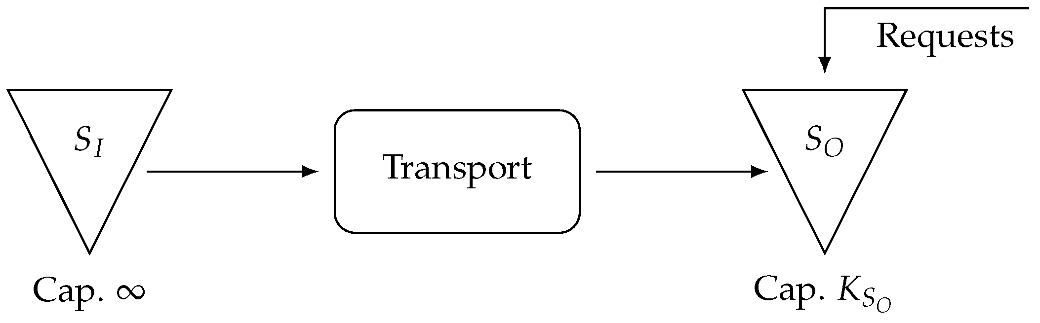
Let us consider a logistics system consisting of two inventory stocks (located in two different companies) with transportation carried out on the road. A schematic of this logistics area is shown in Figure 1.

Input stock $S_I$, assumed to have infinite capacity and to be replenished by each item produced in the upstream system, serves as the source for replenishing output stock $S_O$. The output stock $S_O$, with a finite capacity $K_{S_O}$, fulfills customer requests that arrive at variable intervals following a distribution $\xi \left(t\right)$, while the quantity also varies according to the distribution $\mathsf{\Omega }\left(t\right)$.

To maintain an adequate stock level in $S_O$, transportation is triggered whenever the stock level falls below the predefined threshold ${\lambda }_{S_O}$ allowing for the replenishment of up to N products per transport cycle (corresponding to the vehicle’s maximum capacity). Each transport operation requires a fixed duration of $\tau$ time units before products become available in $S_O$.

There are multiple objectives in the simulation for this example. It is possible to evaluate the performance of the logistics system by analyzing the average stock level of output stock $S_O$ over time. This can provide insights into how well the replenishment process manages demand fluctuations and transport duration. Furthermore, the stockout risk can be determined by monitoring the frequency at which the stock level in $S_O$ falls below the minimum threshold required to trigger transportation. Other indicators, such as transportation efficiency or average transport delay, can be used to assess the effectiveness of the replenishment process, ensuring that transportation is timely and aligned with demand patterns to minimize shortages. Additionally, the utilization rate of transport can be analyzed, reflecting how often the transport capacity is fully utilized relative to demand.

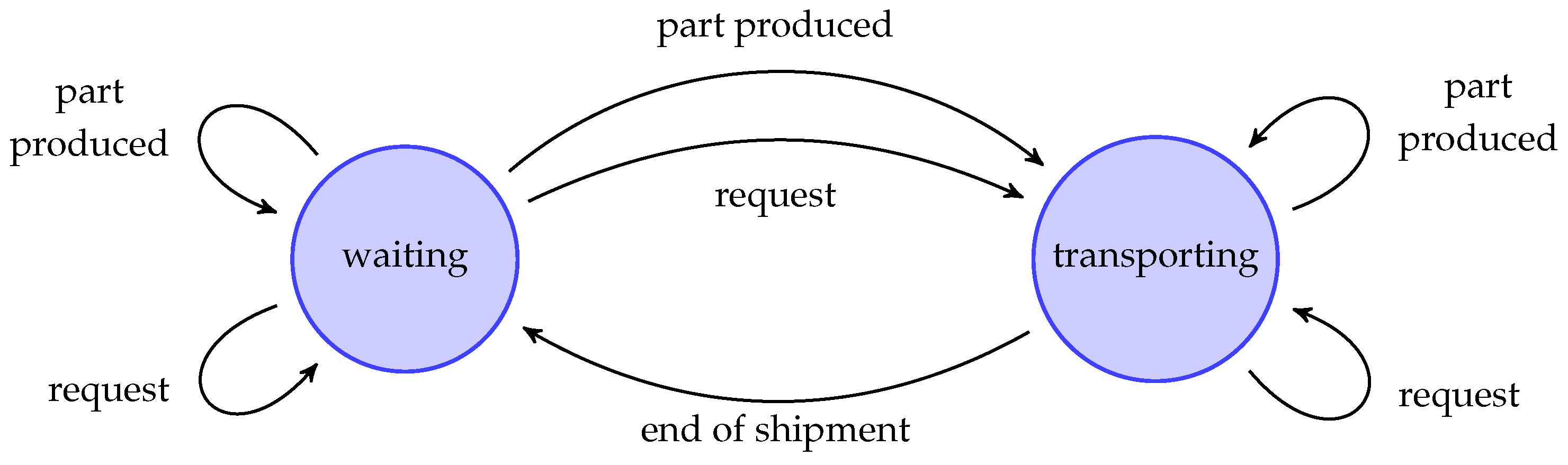
Two events can occur while in the “waiting” state: production of a new part and arrival of a customer request. However, we note that each of these events can either lead to staying in the same state or trigger a transition to the “transporting” state. The transition to the transport state occurs only when all conditions are met, namely, a sufficient quantity available in $S_I$ and a stock level in $S_O$ that is below the threshold ${\lambda }_{S_O}$. In the “transporting” state, the same two events (part production and customer request) may still occur, but they do not affect the state transition. A third event, the completion of the transport operation, triggers the transition back to the “waiting” state.

The set of events can be represented in the form of a state diagram, as shown in Figure 2.

The simulation Algorithm 1 analyzes these two states and the associated events during the simulation period to determine the number of shipments.

In DES algorithms, events are time-driven. Therefore, the conditions if request = true then and if part produced = true then should not be treated as Boolean conditions, but rather as time-based conditions. In this context, how do you determine when an event will occur?

Algorithm 1 Pseudocode of the introductory example

1: Define stocks $S_I$ at level $L_{S_I}$ and $S_0$ at level $L_{S_O}$ 2: Set state as “waiting” 3: Define the arrival of the request based on $\xi \left(t\right)$ and the number of products required based on $\mathsf{\Omega }\left(t\right)$ 4: Start item production 5: Set nbShipments to 0 6: while simulation time is running do 7:     if state = “waiting” then 8:         if request == true then 9:            Define the arrival of the next request based on $\xi \left(t\right)$ and the number of products required based on $\mathsf{\Omega }\left(t\right)$ 10:            if $L{S}_I\ge N$ and $L_{S_O}<{\lambda }_{S_O}$ then 11:                Remove N items from stock $S_I$ 12:                Increment nbShipments by one 13:                Go to “transporting” state for 2$\tau$ time units 14:            end if 15:         else if part produced == true then 16:            Place produced item in stock $S_I$ 17:            Start a new item production 18:            if $L_{S_I}==N$ and $L_{S_O}<{\lambda }_{S_O}$ then 19:                Remove N items from stock $S_I$ 20:                Increment nbShipments by one 21:                Go to “transporting” state for 2$\tau$ time units 22:            end if 23:         end if 24:     else if state = “transporting” then 25:         if request == true then 26:            Define the arrival of the next request based on $\xi \left(t\right)$ and the number of products required based on $\mathsf{\Omega }\left(t\right)$ 27:         else if part produced == true then 28:            Place produced item in stock $S_I$ 29:            Start a new item production 30:         else if end of shipment == true then 31:            Go to “waiting” state 32:         end if 33:     end if 34: end while 35: Display nbShipment

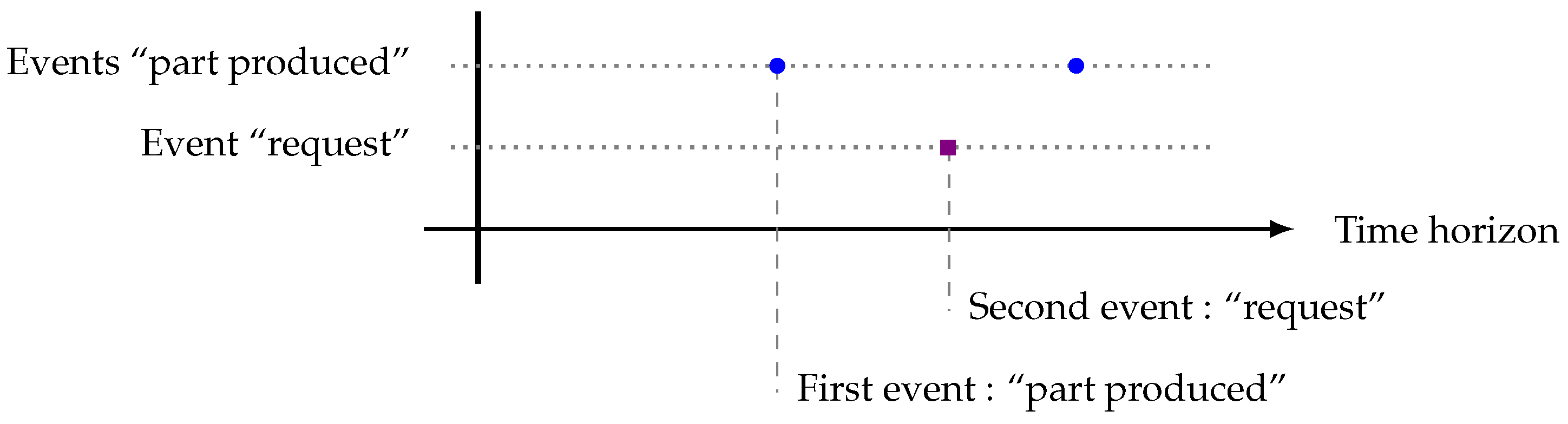
The representation of events over the time horizon is illustrated in Figure 3.

Instinctively, determining which event will occur first is often carried out by testing conditions such as: “if duration before ‘part produced’ < duration before ‘request’ then”. While this method works well for two events, it quickly becomes impractical when dealing with multiple events because it requires the management of numerous conditional statements. A more efficient approach is to use the mathematical function min, in which the arguments represent the time remaining before each event. By subtracting the minimum duration from all event durations, one event will reach zero, whereas the others will retain a strictly positive value. This ensures clear identification of the next event.

Before writing the simulation algorithm based on the state graph (Figure 2), it is essential to clearly define the parameters and variables to be used. The latter are presented in

Table 1. Parameters and variables of the DES algorithm.

Parameter	Variable	Description
$D_{sim}$		Total simulation duration
$T_{sim}$		Simulation clock (current time)
	$state$	Current state of the system
$K_{S_O}$		Maximum stock capacity
	$L{S}_O$	Current stock level
	${\lambda }_{S_O}$	Threshold allowing for the replenishment
	$T_{event}$	Time until next event
$D_{op}$		Operating time
	$T_{op}$	Time remaining until end of part production
$\xi \left(t\right)$		Distribution of request frequency
	$T_{request}$	Time until next request
	N	Number of products delivered per shipment
	$nbShipments$	Total number of shipments

.

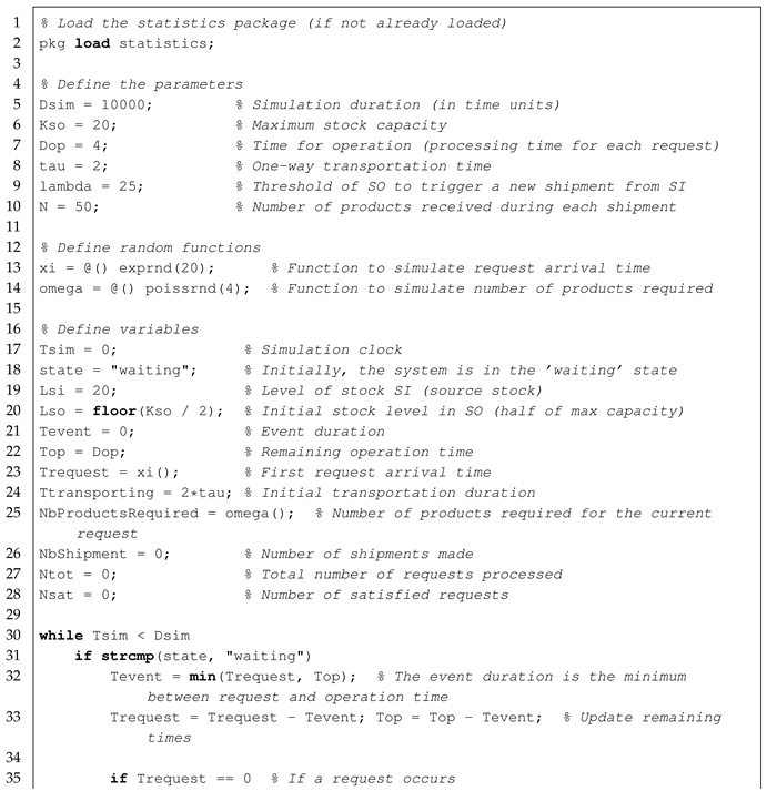
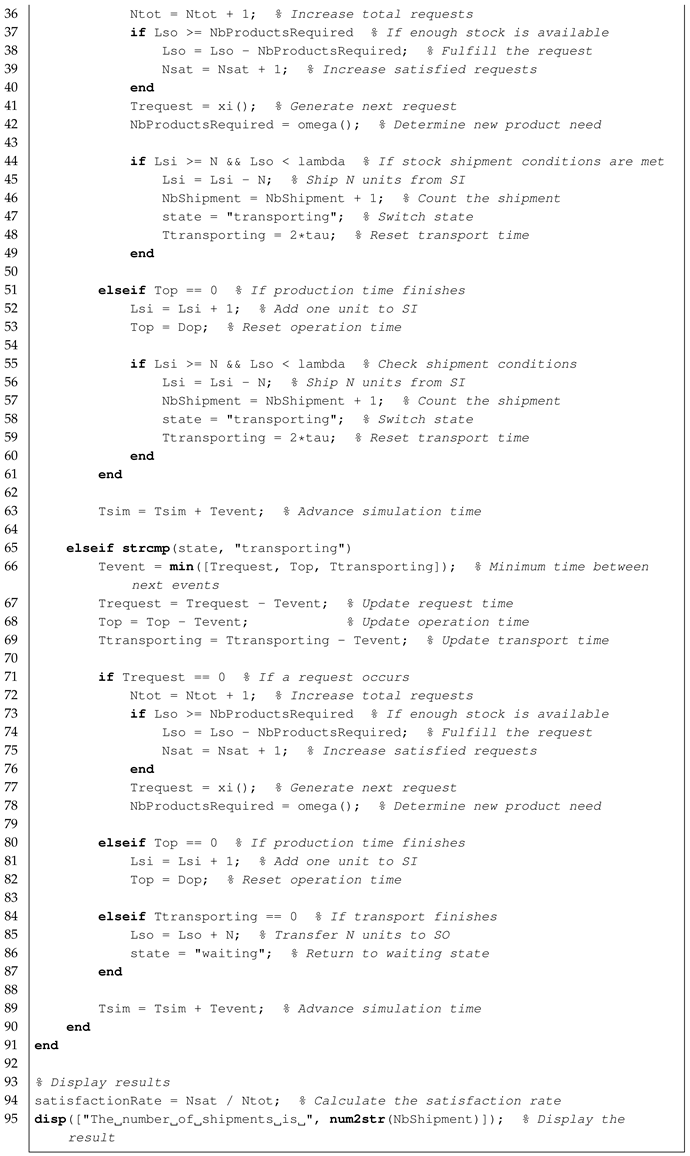
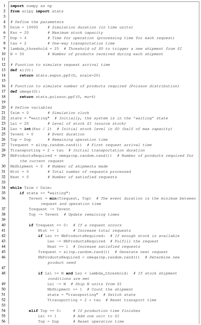
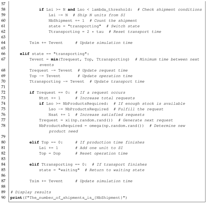
The simulation algorithm that models the system’s behavior, processing events based on the minimum remaining time for each, is presented in Listing A1 (Octave 10.1.0) and Listing A2 (Python 3.13.3) in Appendix A.

The following section models several industrial constraints commonly encountered in supply chain systems, including warehouse management, equipment allocation, maintenance periods, and series and parallel systems. The inclusion of maintenance accounts for downtime periods and repair cycles, whereas the modeling of series and parallel systems reflects the configuration of production lines and resources. In series systems, bottlenecks and dependencies between stages are considered, whereas in parallel systems, resource redundancy and capacity expansion are modeled. By incorporating these elements, the simulation offers a more comprehensive view of the operational challenges within a supply chain, including the production flow, maintenance management, and system configurations.

4. Modeling Industrial Constraints

4.1. Warehouse Management and Equipment Allocation

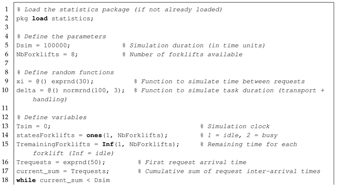
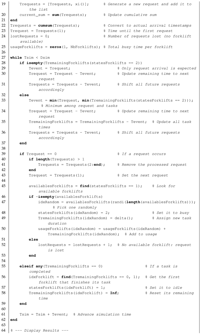
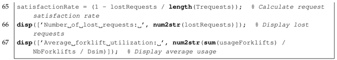
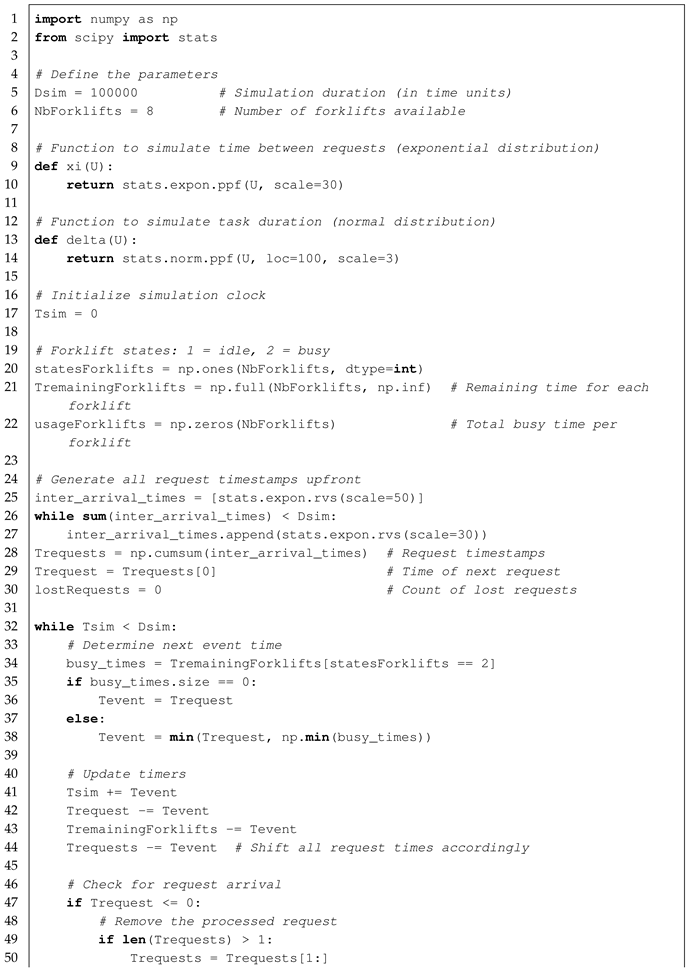
Forklift-based item retrieval systems are a common feature of modern warehouse logistics in which mobile handling units are dynamically assigned to fulfill incoming product requests. This decentralized approach allows for high responsiveness and operational simplicity but also introduces challenges related to resource contention and scheduling efficiency.

In our case, the forklifts are not dedicated to specific warehouse areas. Instead, they are managed independently and each can be in one of two states: idle or busy. When a product request arrives, an idle forklift is selected to retrieve the item, execute the task, and return to an idle state upon completion. However, while each forklift operates autonomously, a central discrete-event simulation coordinates the overall behavior of the system by managing two types of events: the arrival of product requests and completion of forklift tasks.

Different dispatching strategies can be applied to determine which forklift is selected for each request. For example, the system can be expressed by the following options:

• Randomly select an available forklift (as in the current implementation);
• Prefer the one with the lowest cumulative usage;
• Assign the one that has been idle for the longest time.

If no forklift is available at the time a request arrives, the request is considered lost. This basic model can be extended to include delivery time windows, multi-product requests, or zone-based forklift assignments, depending on the complexity of warehouse operations, offering considerable flexibility for future developments.

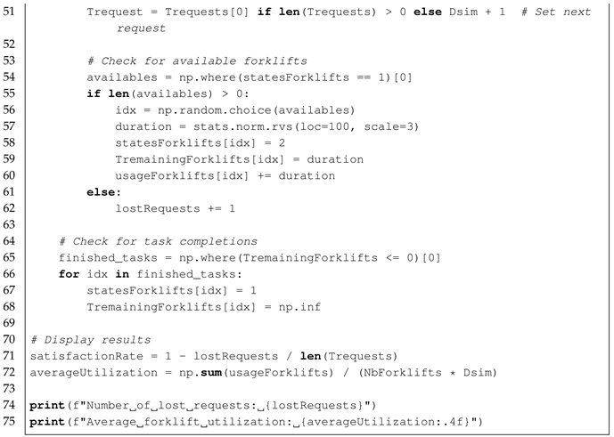
The current simulation aims to evaluate system performance by measuring two key indicators: the number of lost requests due to forklift unavailability and the average utilization rate of forklifts over the simulated period.

The implementation is detailed in Appendix A, with Listing A3 for Octave and Listing A4 for Python.

4.2. Repair Models

A machine subject to failures does not break down randomly but follows a failure law that describes the probability of failure occurrence over time. This law allows one to model the system’s behavior and anticipate its evolution, thereby facilitating the implementation of optimized maintenance strategies. Several common failure laws are used in reliability analysis. For example, the exponential law characterizes systems with random failures, where the Weibull distribution represents different failure regimes (wear and aging), and the normal distribution is often associated with material fatigue phenomena. Understanding these failure laws is crucial for defining appropriate maintenance strategies and minimizing costs and production downtime while ensuring equipment reliability.

Repair models describe the effect of maintenance intervention on the system after failure. They address the following question: what is the impact of the repair?

The most common repair models include the following:

• Perfect repair, which restores the system to an “As Good As New” (AGAN) state.
• Minimal repair, which only restores functionality without improving the system’s overall condition.
• Imperfect repair, which partially restores the system, bringing it to a state between new and old.

4.2.1. Perfect Repair Modeling

The time to failure ($TTF$) of a system is defined as the time elapsed before the first failure occurs when the system is considered to be new. This time can be generated using the inverse cumulative distribution method. This technique involves applying the quantile function (or inverse cumulative distribution function) of a given probability distribution to a random variable that is uniformly distributed over the interval $[0,1]$. Specifically, if U is a random variable uniformly distributed over $[0,1]$ and $F^{-1}$ is the quantile function associated with the chosen failure distribution (e.g., exponential, Weibull, log-normal), $TTF$ is obtained through the transformation $T=F^{-1}\left(U\right)$. This method ensures that the simulated values comply with specified failure laws.

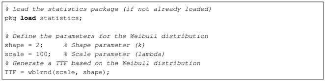
In Octave, the “statistics” package provides functions to directly generate a time to failure ($TTF$) data. The exprnd function generates $TTF$ based on an exponential distribution, wblrnd generates $TTF$ based on a Weibull distribution, and normrnd generates $TTF$ based on a normal distribution, making it easy to simulate failure times according to these different distributions. For example, the following Octave code (Listing 1) demonstrates how to generate a $TTF$ based on a Weibull distribution with shape parameter 2 and scale parameter 100.

Listing 1. Octave code to generate a time to failure based on the Weibull distribution.

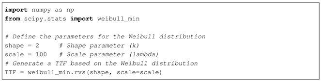
In Python, the “scipy.stats” module offers built-in functions for generating $TTF$ from various probability distributions. The function expon.rvs allows sampling from an exponential distribution, weibull_min.rvs generates values following a Weibull distribution, and norm.rvs produces failure times based on normal distribution. These functions make it straightforward to simulate the different failure patterns. Listing 2 presents a Python implementation that generates a $TTF$.

Listing 2. Python code to generate a time to failure based on the Weibull distribution.

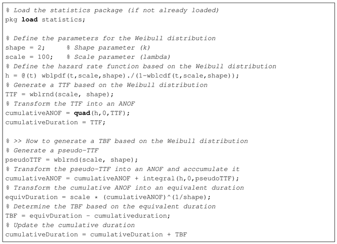
4.2.2. Minimal Repair Modeling

Modeling the time between failures ($TBF$) with minimal repairs is more complex than that with perfect repairs because it requires considering the history of past failures. While perfect repairs restore the system to a “new” state, minimal repairs provide only partial restoration, increasing the likelihood of future failures. Consequently, failure frequency increases over time, making it essential to account for previous failures when predicting future failures. This historical dependence makes the failure distribution time-dependent, reflecting accumulated wear and tear, and necessitates a model that incorporates this cumulative effect for an accurate reliability analysis.

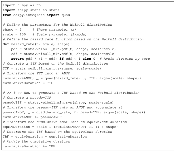
This approach involves transforming the time to failure ($TTF$) and any previous time between failures ($TBF$) into an average number of failures (ANOF) using the hazard rate function $h\left(t\right)$. This is achieved by integrating the hazard rates over time. Once the $ANOF$ is obtained, these failures are accumulated to calculate the total duration. To generate the new $TBF$, a pseudo-$TTF$ is first generated using the previous method (involving the inverse transformation of the hazard rate function), which is then converted into the average number of failures. This value is then added to the cumulative ANOF. Subsequently, the inverse process is applied by converting the average number of failures into the total duration. The previously calculated $TTF$ and $TBF$ values are then subtracted from this duration to account for the cumulative effect of past failures. This methodology allows for the accurate modeling of failure patterns and helps adjust predictions for the remaining lifetime of the system, factoring in the history of prior failures.

Listings 3 and 4 show how to code minimum repairs using Octave and Python, respectively. It is necessary to maintain two variables during the simulation, intended for cumulative $ANOF$ and cumulative duration ($TTF$ + $\mathsf{\Sigma }$$TBF$).

Listing 3. Octave code to generate a time between failures based on the Weibull distribution.

Listing 4. Python code to generate a time between failures based on the Weibull distribution.

4.2.3. Imperfect Repair Modeling

Imperfect repairs introduce additional complexity in reliability modeling, as they only partially restore the system after failure. Unlike perfect repairs, which reset the system to a “new” state, or minimal repairs, which maintain the failure rate at the same level as just before the failure, imperfect repairs result in an intermediate condition in which the system retains some wear from prior usage. These repairs can be modeled in various ways, depending on the assumptions made regarding their effects on the degradation of the system. Common approaches include the age reduction model, where the system’s effective age is reduced but not reset to zero; the intensity reduction model, which decreases the failure rate without altering the system’s age; and hybrid models, which combine aspects of both approaches [43].

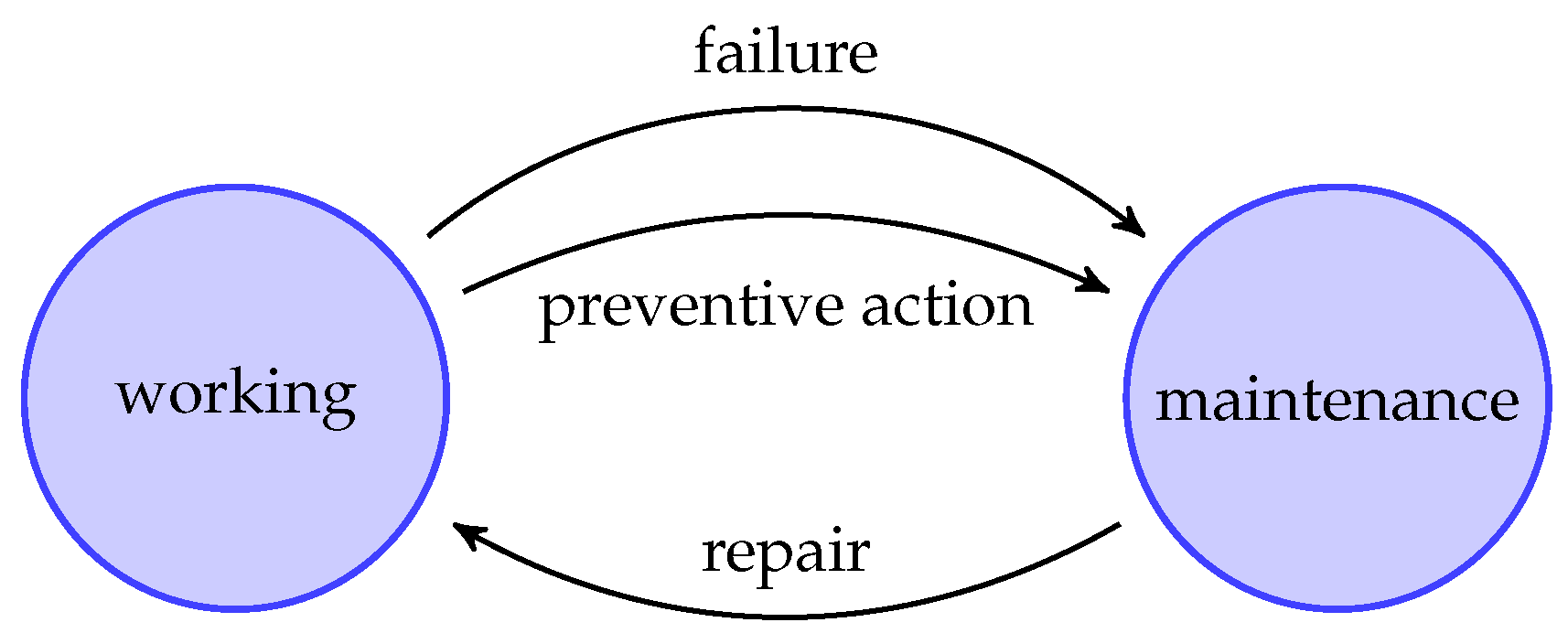
4.3. Preventive Maintenance Policies

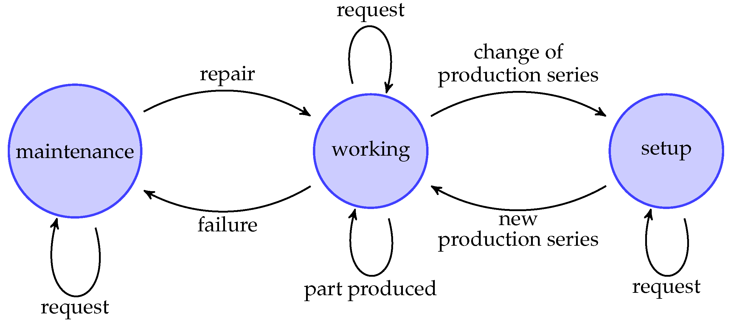
Preventive maintenance policies are crucial to ensure the reliability and performance of production systems and supply chains. These policies aim to minimize the average costs and/or downtime while extending the lifespan of equipment by scheduling maintenance activities at predetermined intervals. Two common strategies used for preventive maintenance are age-based and block-based. These strategies are designed to optimize maintenance schedules based on either the operational age of the equipment or fixed time intervals. The state diagram for preventive maintenance policies, which outlines these strategies, is shown in Figure 4.

4.3.1. Age-Based Strategy

With an age-based strategy, preventive maintenance is scheduled based on the age of the equipment. For example, a component is replaced once it reaches a predefined operating time, either after failure or after previous preventive maintenance.

An example of pseudocode for the age-based preventive maintenance strategy is given in Algorithm 2. The aim is to determine the average maintenance cost per unit time. This cost is computed based on corrective costs (fixed) and preventive costs (fixed).

4.3.2. Block-Based Strategy

With a block-based strategy, preventive maintenance is performed at fixed time intervals, regardless of the individual operating time of each piece of equipment. This strategy is often used to simplify scheduling and optimize resource management.

The pseudocode is largely similar to that of Algorithm 2. The only difference is the reset date for preventive maintenance. The age-based strategy is reset after the last preventive maintenance or following a failure. Therefore, it is reset when exiting the maintenance state. In the block strategy, reset occurs only after preventive maintenance. Therefore, the modification involves moving line 18 after line 13.

Algorithm 2 Pseudocode for the age-based preventive maintenance strategy

1: Define corrective cost: $C_C$ 2: Define preventive cost: $C_P$ 3: Define the TTF based on distribution $f\left(t\right)$ 4: while simulation time is running do 5:     if state = ‘working’ then 6:         Wait during the min time between TTR and $\tau$ 7:         if failure = true then 8:            Go to state “maintenance” 9:            Define the TTR based on distribution $g_C\left(t\right)$ 10:            Increment total cost with $C_C$ 11:          else if preventive action = true then 12:            Go to state “maintenance” 13:            Define the TTR based on distribution $g_P\left(t\right)$ 14:            Increment total cost with $C_P$ 15:          end if 16:     else if state = “maintenance” then 17:         Wait during the TTR 18:         Define the next date $\tau$ of preventive action 19:         Go to state “working” 20:     end if 21: end while 22: Display ${\displaystyle \frac{\mathrm{total}\cos \mathrm{t}}{\mathrm{simulation}\mathrm{duration}}}$

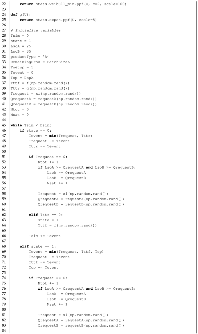
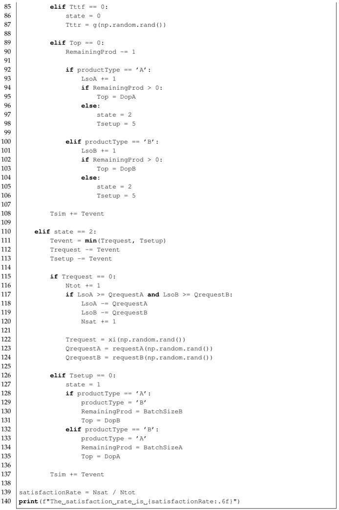
4.4. Batch Production

Batch production is a manufacturing process in which products are produced in discrete groups or batches rather than in a continuous flow. This approach is widely used in industries where products share similarities but may differ in specifications or quantities. Although batch production offers flexibility in handling multiple product types and optimizing resource utilization, it also requires careful planning to mitigate inefficiencies related to setup times and inventory imbalances. Effective management of batch transitions is crucial for minimizing production downtime, avoiding excessive stock levels, and ensuring a stable supply of components. These constraints can affect the overall efficiency and throughput, making it essential to carefully balance batch sizes, production schedules, and resource allocation to maintain optimal performance.

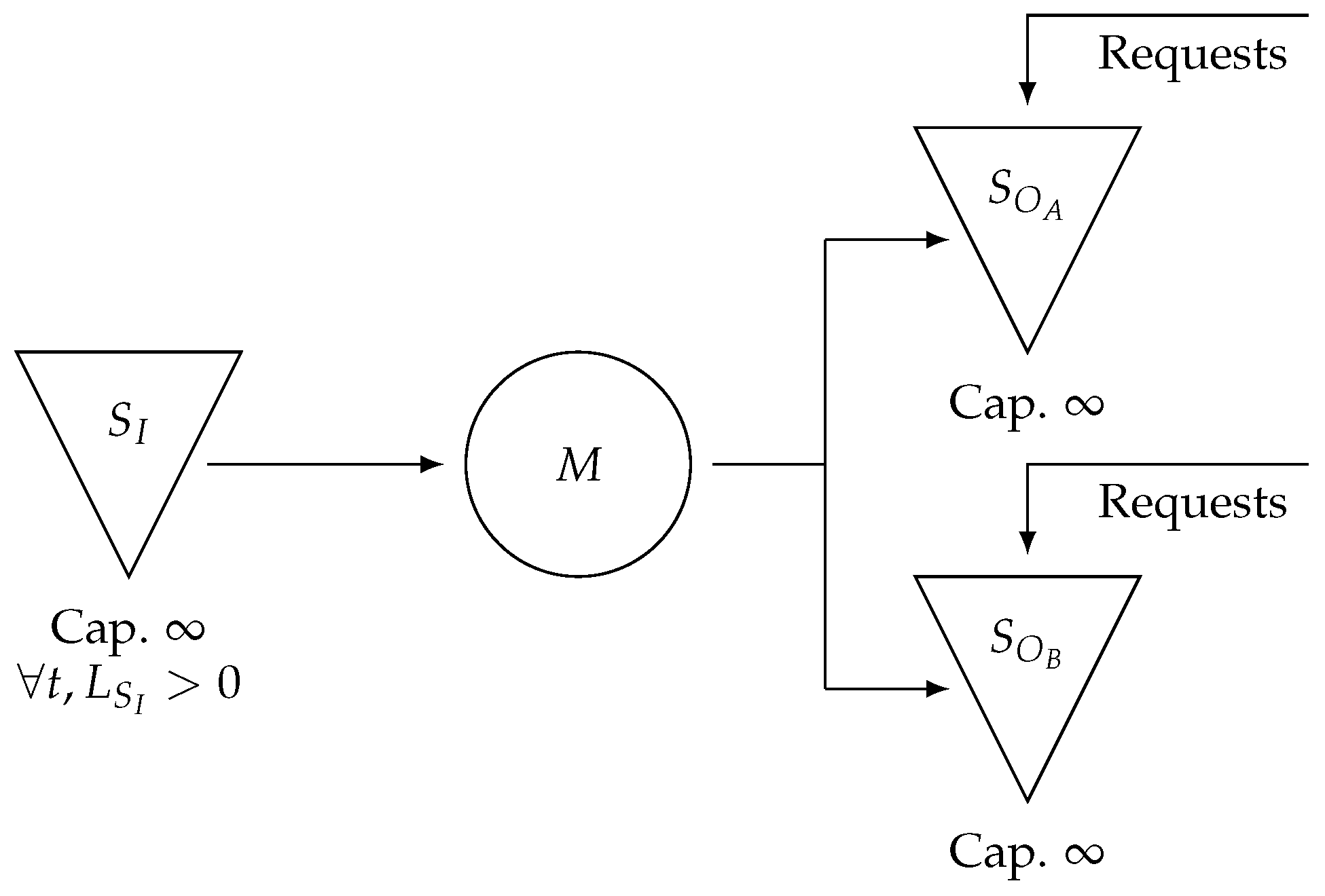
The system illustrated in Figure 5 represents a section of a production system comprising a single machine and two downstream storage units with an infinite capacity (input stock level ($L_{S_I}$) is always positive). These storage units hold finished parts of types A and B produced in batch sizes $BatchSizeA$ and $BatchSizeB$, respectively. Because the machine can only produce one type of part at a time, switching between batches incurs a setup time, which directly affects the system performance. If batches are too small, frequent setups reduce production efficiency and increase the risk of stock shortage. Conversely, overly large batches can lead to inventory imbalances, where one part accumulates in excess while the other runs out, disrupting the fulfillment of customer requests.

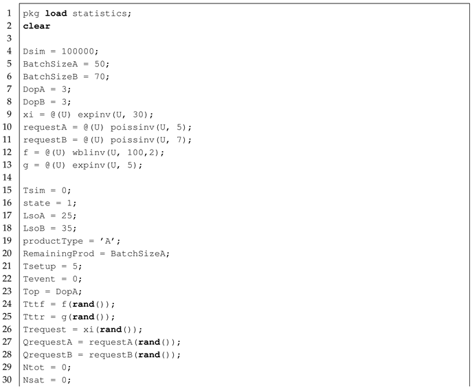
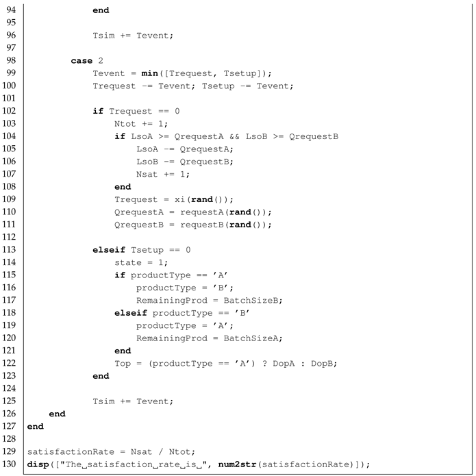
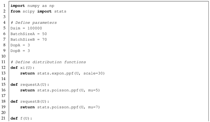
Customer requests arrive at variable intervals following the distribution $\xi \left(t\right)$, with order quantities varying according to Poisson distributions denoted by $requestA\left(t\right)$ and $requestB\left(t\right)$. Machine M is subject to random failures, governed by the failure distribution $f\left(t\right)$, whereas repair times follow the distribution $g\left(t\right)$. The corresponding state diagram is shown in Figure 6 and the code for this system is provided in Appendix A, with Listing A5 for Octave and Listing A6 for Python.

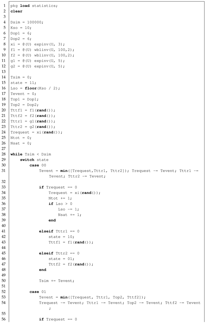
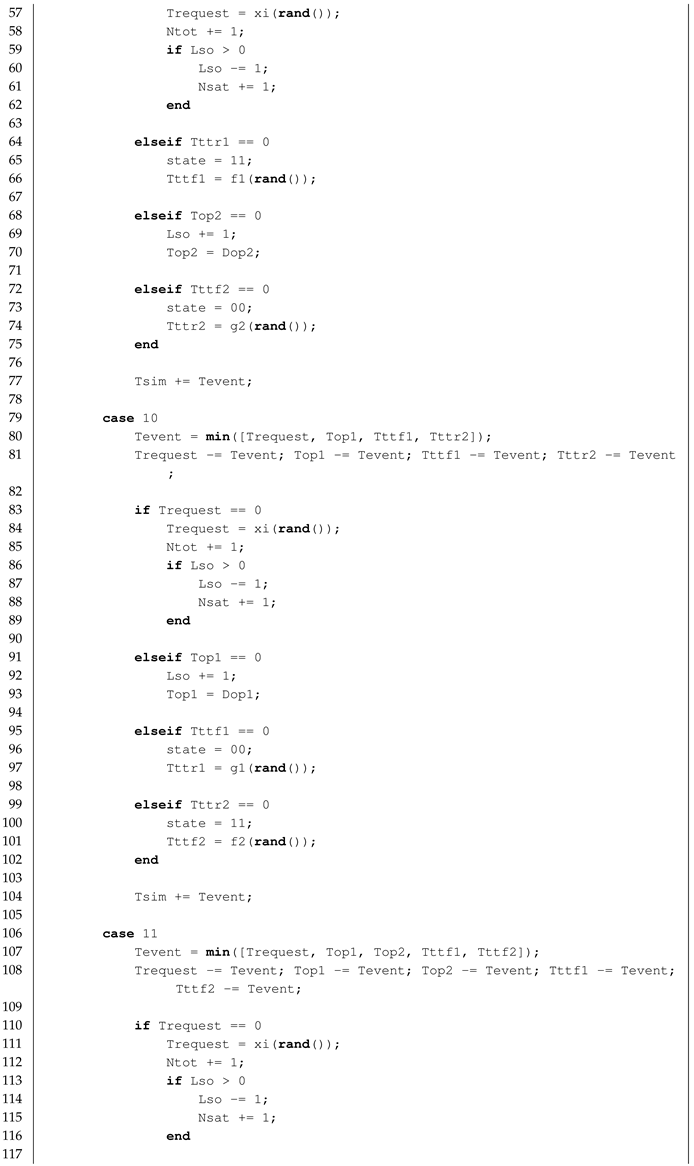
4.5. System Configuration: Parallel and Serial Systems

Understanding the structure of a production system is essential for analyzing its performance and reliability. Production systems can generally be classified into series and parallel configurations, each of which presents distinct operational characteristics and challenges. In a series system, machines operate sequentially, meaning that the failure or slowdown of one machine directly affects the overall production flow. In contrast, a parallel system consists of multiple machines performing the same task simultaneously, ensuring redundancy and increased throughput, because production can continue even if one machine fails. Kusma et al. proposed a safety maturity model for occupational health in the environment of Industry 4.0, emphasizing the role of digital tools such as DES in addressing technical and human-centric challenges. This connection reinforced the adaptability of simulation tools to modern production systems [44].

4.5.1. Parallel System

As depicted in Figure 7, the parallel system involves two machines, $M_1$ and $M_2$, both of which are drawn from input stock $S_I$ with infinite capacity and continuous replenishment. Each machine operates independently and processes products during its respective operational duration $D_{o{p}_1}$ and $D_{o{p}_2}$. Upon the completion of their operations, both machines transfer the finished products to output stock $S_O$, which has an infinite capacity. The output stock is responsible for fulfilling external demand requests that arrive at variable intervals, with a fixed quantity of one per request, and follows the distribution $\xi \left(t\right)$.

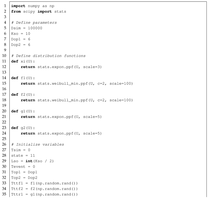
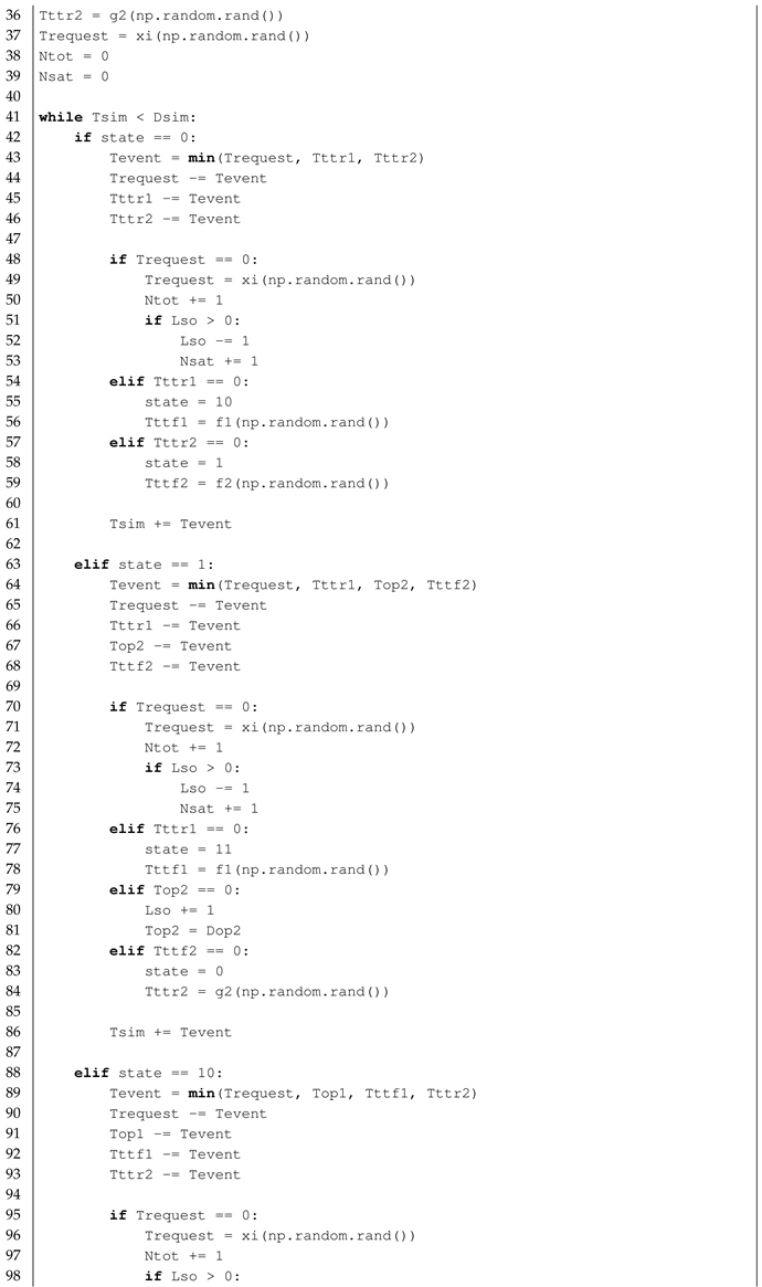
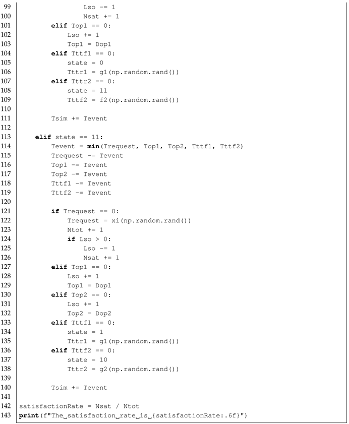
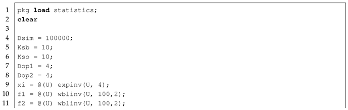
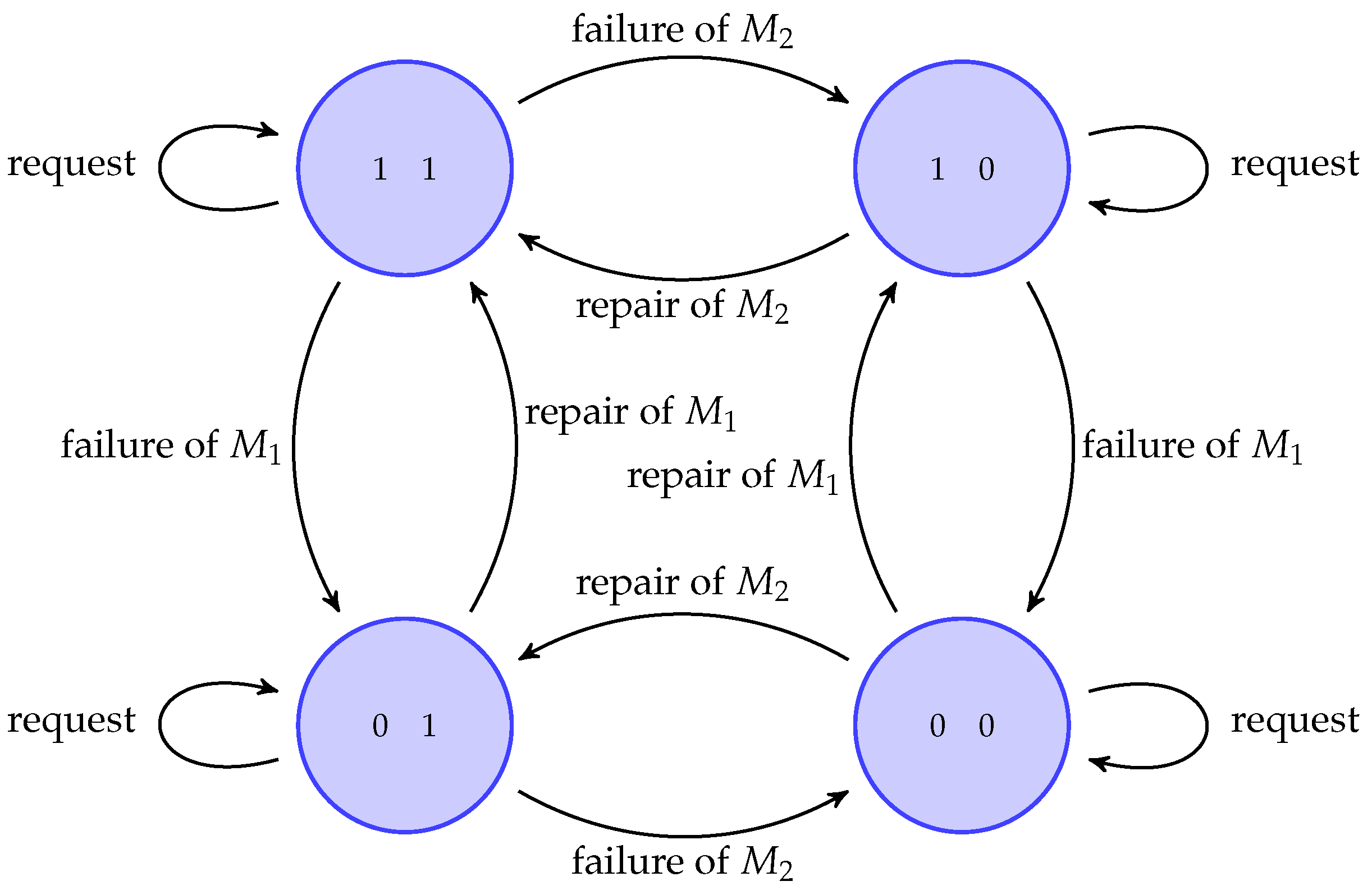
Both machines $M_1$ and $M_2$ are subject to random failures, and their failure times are governed by the distributions $f_1\left(t\right)$ and $f_2\left(t\right)$, respectively. These failures are based solely on the operational usage of machines. When a failure occurs, machine $M_i$ ($i=1,2$) is immediately repaired with a repair time based on the distributions $g_i\left(t\right)$. The parallel nature of the system ensures that the failure of one machine does not halt production, as the other machine can continue to process and supply products to the output stock.

The objective of this simulation remains the same as in the introductory example: the determination of the customer satisfaction rate.

For clarity, the states “working” and “maintenance” are replaced by the notations “1” and “0”, respectively, in the state diagram (Figure 8). Thus, the state “10” indicates that $M_1$ is operating while $M_2$ is under maintenance.

The code for this system is provided in Appendix A, with Listing A7 for Octave, and Listing A8 for Python.

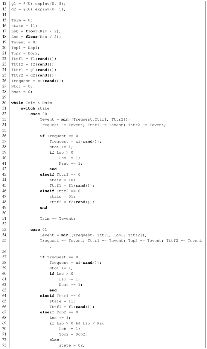
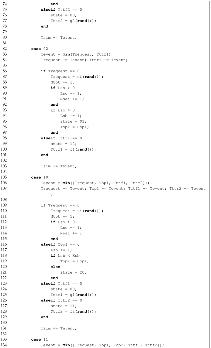
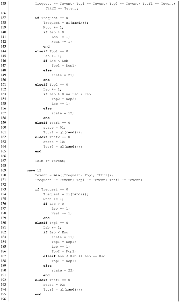
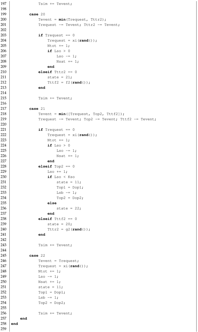
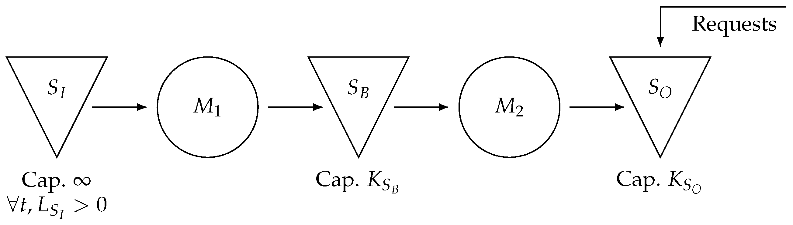
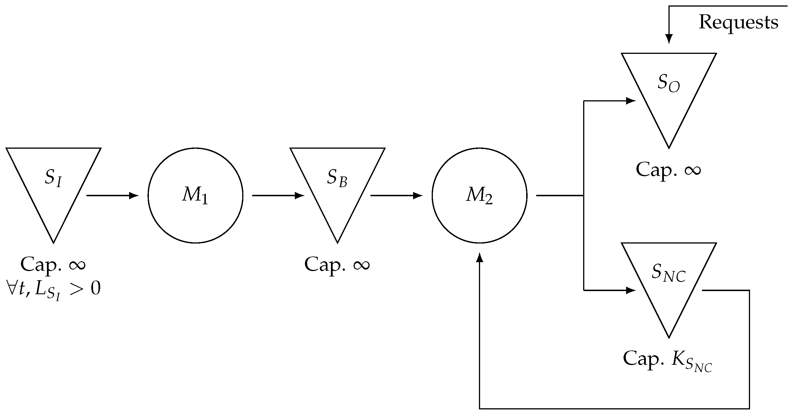
4.5.2. Series System

As illustrated in Figure 9, the series system consists of two machines, $M_1$ and $M_2$. Machine $M_1$ is supplied from input stock $S_I$ with infinite capacity and continuous replenishment. After operational duration $D_{o{p}_1}$, semi-finished products are transferred to a finite-capacity intermediate stock $K_{S_B}$, which supplies machine $M_2$ on demand. This second machine processes the products within operational duration $D_{o{p}_2}$ before depositing them into the final stock, which has a capacity of $K_{S_O}$. This stock fulfills external requests that arrive at variable intervals according to the distribution $\xi \left(t\right)$ with a fixed demand quantity of one.

Machines $M_i$$(i=1,2)$ are subject to random failures with the time to failure following the distribution $f_i\left(t\right)$. These failures are solely based on machine usage. Failures are immediately taken over by the maintenance service, and repair durations follow the distributions $g_i\left(t\right)$.

Again, we aim to determine the customer satisfaction rate as the objective of this simulation.

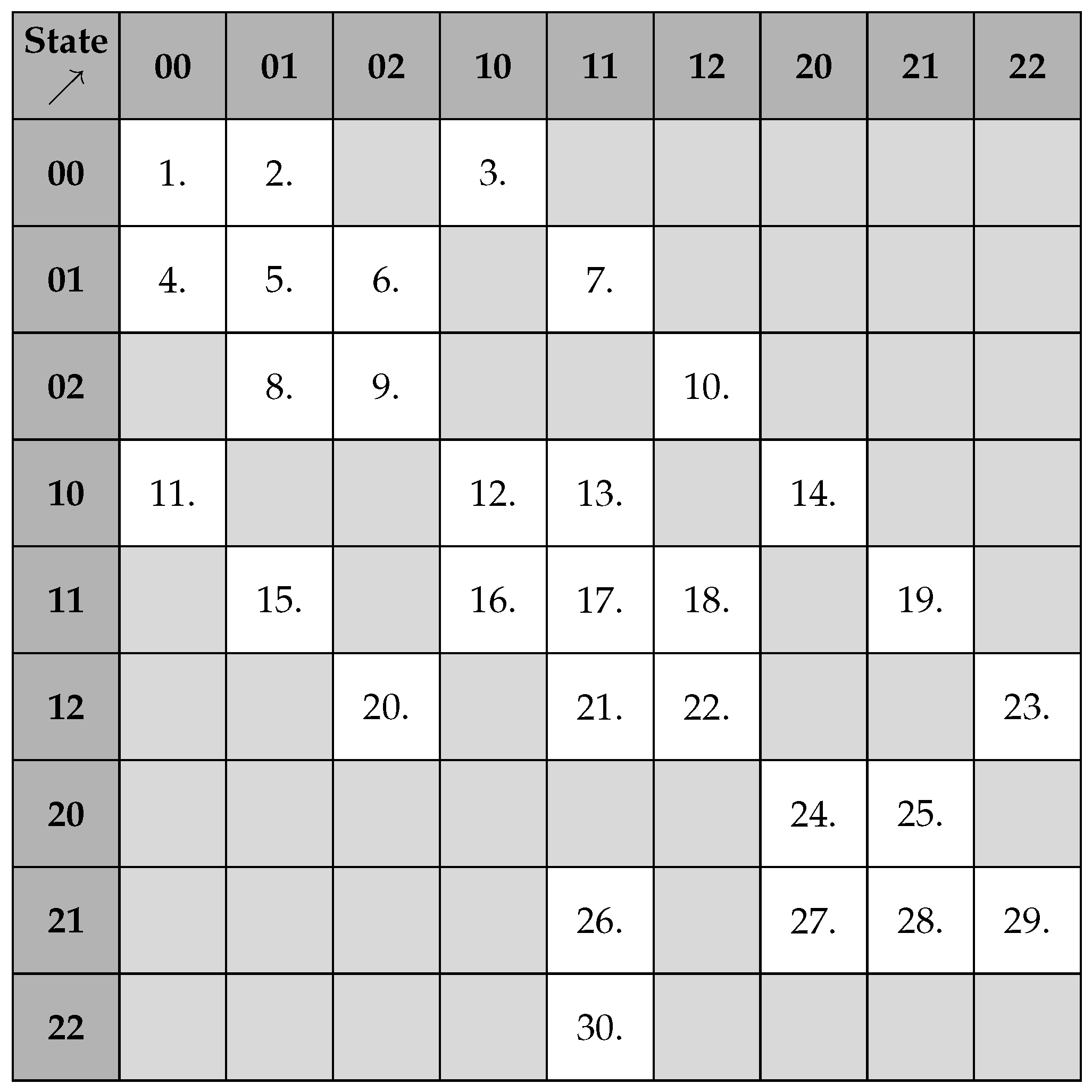
Given the series structure and finite stock capacities of the system, the number of states and their interactions make a state graph complex and difficult to interpret. Instead of a graphical representation, events and state transitions were structured using both a matrix (Figure 10) and a list format (presented below), which were chosen as the most suitable approaches.

Each machine can be in one of the three states: (1) working, (2) maintenance, or (3) standby. As the system consists of two machines, this results in nine possible state combinations, leading to 81 distinct transitions.

All the inter-state and intra-state transitions represented in the matrix (Figure 10) are detailed below. By definition, events are time-driven, but additional conditions (highlighted in the list below) may also influence transitions. These conditions have been outlined for clarity.

• State “00” to…
  • State “00”: request
  • State “01”: repair of $M_2$
  • State “10”: repair of $M_1$
• State “01” to…

  4.

  State “00”: failure of $M_2$

  5.

  State “01”: request || part produced on M₂ && Lsb > 0 && Lso < Kso

  6.

  State ’02”: part produced on M₂ && (Lsb == 0 || Lso == Kso)

  7.

  State “11”: repair of $M_1$

• State “02” to…

  8.

  State “01”: request && Lsb > 0

  9.

  State “02”: request && Lsb == 0

  10.

  State “12”: repair of $M_1$

• State “10” to…

  11.

  State “00”: failure of $M_1$

  12.

  State “10”: request || part produced on $M_1$ && Lsb < Ksb

  13.

  State “11”: repair of $M_2$

  14.

  State “20”: part produced on $M_1$ && Lsb == Ksb

• State “11” to…

  15.

  State “01”: failure of $M_1$

  16.

  State “10”: failure of $M_2$

  17.

  State “11”: request || part produced on $M_1$ && Lsb < Ksb || part produced on $M_2$ && Lsb > 0 && Lso < Kso

  18.

  State “12”: part produced on $M_2$ && (Lsb > 0 || Lso < Kso)

  19.

  State “21”: part produced on $M_1$ && Lsb == Ksb

• State “12” to…

  20.

  State “02”: failure of $M_1$

  21.

  State “11”: part produced on $M_1$ && Lso < Kso

  22.

  State 12”: request || part produced on $M_1$ && Lsb < Ksb && Lso == Kso

  23.

  State “22”: part produced on $M_1$ && Lsb == Ksb && Lso == Kso

• State “20’ to…

  24.

  State “20”: request

  25.

  State “21”: repair of $M_2$

• State “21” to…

  26.

  State “11”: part produced on $M_2$ && Lso < Kso

  27.

  State “20”: failure of $M_2$

  28.

  State “21”: request

  29.

  State “22”: part produced on $M_2$ && Lso == Kso

• State “22” to…

  30.

  State “11”: request

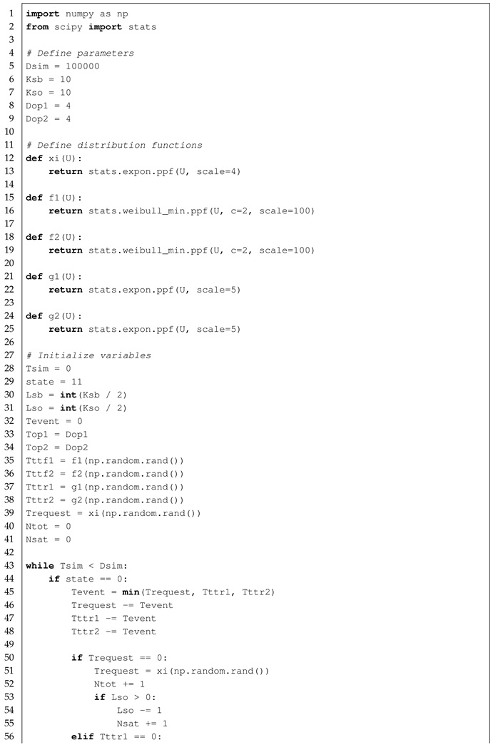
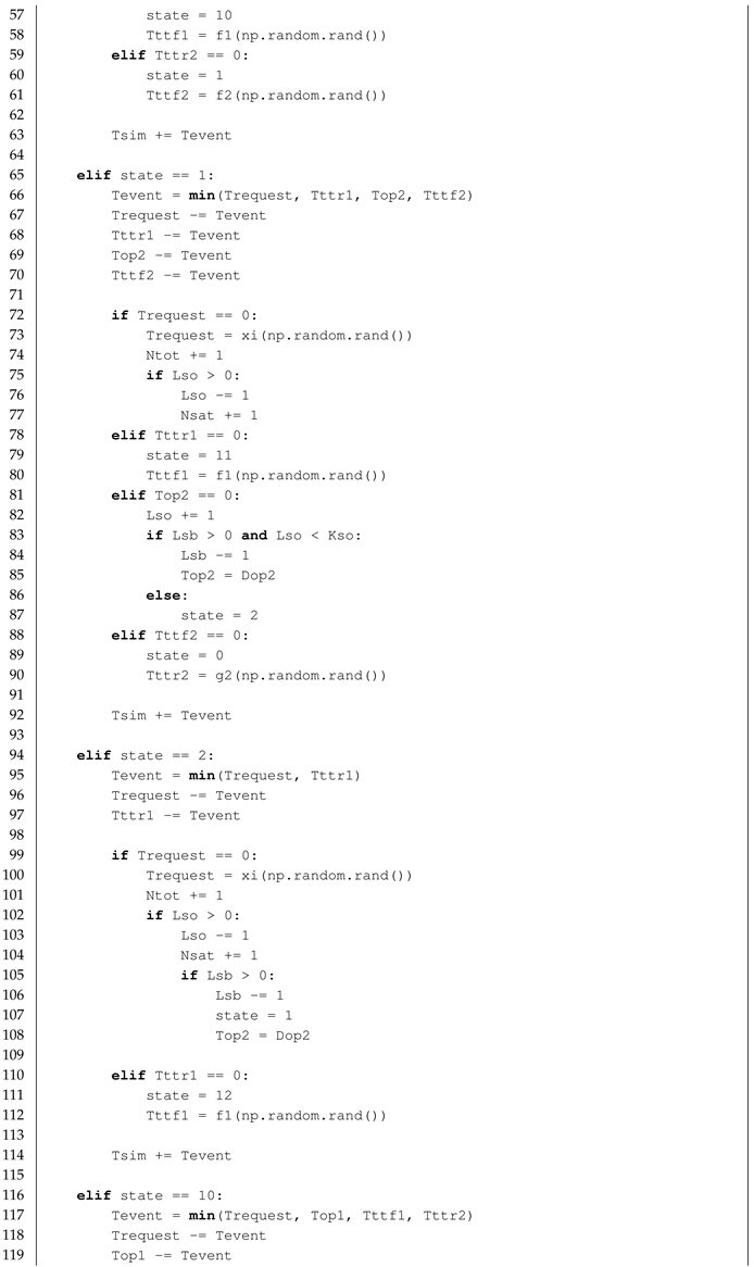
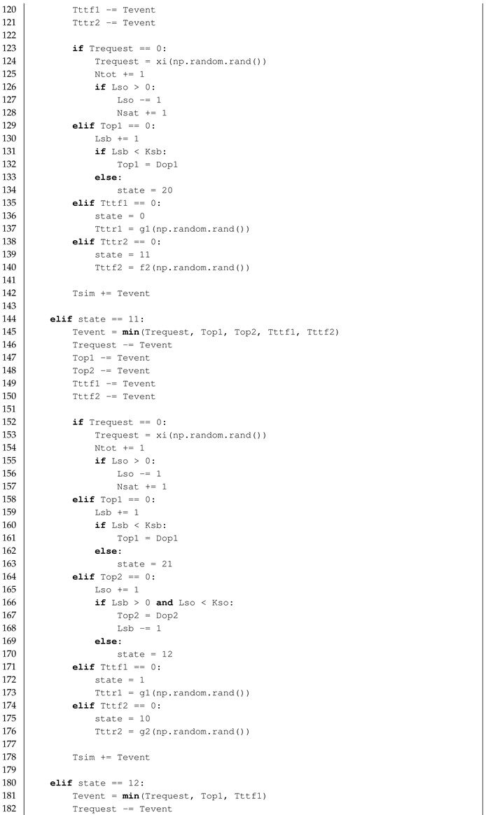
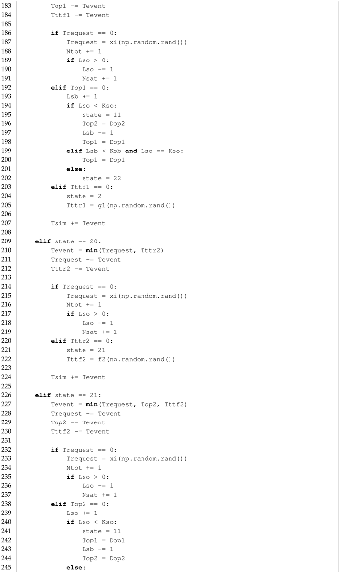
The code for this system is provided in Appendix A, with Listing A9 for Octave, and Listing A10 for Python.

In this section, we explore the key production constraints, including system typology, preventive maintenance policies, and batch production, along with their respective modeling and implementation approaches. By structuring these constraints within discrete-event simulation frameworks, we establish a solid foundation for analyzing complex manufacturing systems. The methodologies and coding principles presented herein provide the necessary tools for tackling practical exercises. In the next Section 5, these concepts are applied to a concrete scenario, allowing for hands-on exploration and a deeper understanding of production system dynamics.

5. Practicing

5.1. Remanufacturing System Coupled with Maintenance and Quality Management

Consider a production system consisting of two machines in series, denoted by $M_1$ and $M_2$. Machine $M_1$ is continuously supplied by input stock $S_I$, which can never be depleted, and produces semi-finished products stored in $S_B$. These semi-finished products are then processed using machine $M_2$. However, the manufacturing process on $M_2$ is delicate, leading to 8% of products being nonconforming. These defective products are placed in stock $S_{NC}$, whereas the conforming products are stored in $S_O$, which has infinite capacity and can accommodate all finished products (Figure 11).

The operating times of machines $M_1$ and $M_2$ are denoted by $D_{O{p}_1}$ and $D_{O{p}_2}$, respectively, with $D_{O{p}_2}$ applied to the products from both $S_B$ and $S_{NC}$. When stock $S_{NC}$ reaches its maximum capacity, $K_{S_{NC}}$, non-conforming products must be reprocessed by $M_2$ after an adjustment period, ${\mu }_A$. Similarly, switching machine $M_2$ back to processing semi-finished products from $S_B$ requires the same adjustment time, ${\mu }_A$.

Both machines $M_1$ and $M_2$ are subject to random failures, with failure durations following the distributions $f_1\left(t\right)$ and $f_2\left(t\right)$, respectively. To minimize downtime owing to corrective maintenance, an age-based preventive maintenance strategy is implemented for each machine. A single maintenance technician is available on-site. However, if both machines require simultaneous maintenance (either corrective or preventive), a second technician is temporarily called in, introducing an additional delay ${\mu }_S$. The corrective maintenance durations are denoted by ${\mu }_C$, whereas the preventive maintenance durations are represented by ${\mu }_P$, with no distinction between the two machines in terms of these durations. Maintenance operations incur fixed costs $C_C$ and $C_P$ for corrective and preventive maintenance, respectively. Finally, each product stored in $S_B$ or $S_{NC}$ for one unit of time incurs storage cost $C_S$, whereas each conforming finished product generates profit P.

The objective of this work is to estimate the gain (profit minus expenses) of the production area based on the data provided in

Table 2. Parameters of the practice exercise.

Parameter	Value	Comment
$D_{sim}$	100,000	Duration of simulation time horizon
$K_{S_{NC}}$	20	Maximum capacity of non-conforming stock
$D_{O{p}_1}$	4	Processing time on machine $M_1$
$D_{O{p}_2}$	4	Processing time on machine $M_2$
$f_1$	W(100, 2)	Weibull distribution with
$f_2$	W(100, 2)	Scale (100) and shape (2) parameters
Compliance rate	0.08
${\mu }_A$	5	Adjustment time when switching processing modes
${\mu }_C$	5	Duration of corrective maintenance
${\mu }_P$	3	Duration of preventive maintenance
${\mu }_S$	1.5	Delay when second technician is called
$C_C$	300	Cost per corrective maintenance
$C_P$	100	Cost per preventive maintenance
P	275	Profit per conforming product
$C_S$	0.05	Storage cost for $S_B$ and $S_{NC}$
$ag{e}_1$	70	Preventive maintenance intervals on $M_1$
$ag{e}_2$	70	Preventive maintenance intervals on $M_2$

.

To successfully tackle this exercise, the recommended steps are as follows:

• Identify the system states, events, and related conditions. Representing these in a state diagram can facilitate the writing of the algorithm.
• Identify the parameters and initialize the variables.
• Write the simulation algorithm.

5.2. Transport Logistic Function

Consider a logistics system responsible for transporting goods from central warehouse W to three regional distribution centers, denoted as $D_1$, $D_2$, and $D_3$. The warehouse operates a fleet of homogeneous trucks, each with a maximum capacity $Q_T$ and fixed loading/unloading time ${\mu }_L$ at both the warehouse and distribution centers. Each truck departs from the warehouse, delivers goods to one or more destinations, and returns to W for the next assignment.

Customer demand at each distribution center is stochastic and follows independent time-varying Poisson processes with rates ${\lambda }_1\left(t\right)$, ${\lambda }_2\left(t\right)$, and ${\lambda }_3\left(t\right)$, respectively. Whenever a demand event occurs at a distribution center, the system updates its transport plan to ensure that stockouts are minimized. If the inventory level at any center falls below the safety threshold $s_i$ ($i\in \{1,2,3\}$), an urgent delivery request is triggered.

Transport routes are subject to variable travel times $T_{ij}$ depending on the current traffic conditions and the distance between W and each $D_i$, with $T_{ij}$ following time-dependent distributions $f_{ij}\left(t\right)$ ($i\in \{1,2,3\},j$ denotes time windows). Additionally, transport costs are incurred per kilometer traveled ($C_{km}$), and each delivery that satisfies an urgent request yields bonus revenue $R_U$, while each stockout incurs a penalty cost $C_{SO}$.

The truck dispatching policy is rule-based: at each decision point (e.g., a truck returns to W or a new urgent request is received), the system assigns trucks based on a priority score combining the current inventory levels, demand forecasts, and expected travel time. If no trucks are available, the system can temporarily rent an external vehicle at a higher cost, $C_R$, but with no loading delay.

All inventory levels, truck statuses (available, en route, loading/unloading), and customer demands were tracked over time. The simulation is used to evaluate the performance of the transportation function over horizon $T_H$, with key performance indicators including the total cost, number of stockouts avoided, truck utilization rates, and percentage of urgent deliveries fulfilled within acceptable time frames.

The objective of this simulation is to assess the cost-effectiveness and reactivity of the transportation system based on the data provided in

Table 3. Input parameters for the logistics transport simulation.

Parameter	Value	Comment
$Q_T$	100	Truck capacity
${\mu }_L$	20	Loading/unloading time per location
${\lambda }_1\left(t\right)$, ${\lambda }_2\left(t\right)$, ${\lambda }_3\left(t\right)$	Time-varying Poisson	Demand rate at each distribution center
$s_i$	50	Safety stock threshold for each $D_i$
$T_{ij}$	$\mathcal{N}({\mu }_{T_{ij}},{\sigma }_{T_{ij}}^2)$	Travel time (warehouse to $D_i$), traffic-dependent
$f_{ij}\left(t\right)$	Empirical or Gaussian	Distribution of $T_{ij}$ depending on time of day
$C_{km}$	1.25	Cost per kilometer traveled
$C_{SO}$	75	Penalty for stockout event
$R_U$	20	Bonus for urgent delivery fulfilled on time
$C_R$	150	Cost for renting an external truck
$T_H$	300	Total simulation horizon

and to test the robustness of the dispatching policy under different demand and traffic scenarios.

To successfully carry out this exercise, the recommended steps are as follows:

• Identify the key events (e.g., demand arrivals, truck departures/arrivals, stockout occurrences) and system states (e.g., inventory levels, truck locations).
• Define the stochastic parameters and initialize simulation variables.
• Write and validate the event-based simulation algorithm.

5.3. Warehousing Management

Consider a warehouse facility organized into several storage zones: receiving area $Z_R$, picking area $Z_P$, and reserve storage area $Z_S$. Pallets of goods arrive at the warehouse via inbound trucks and are first unloaded in $Z_R$, where they are identified and sorted before being stored in $Z_P$ or $Z_S$ depending on their rotation class (high or low). High-turnover items are placed in $Z_P$ for quick picking, whereas the others are stored deeper in $Z_S$.

The movement of pallets within a warehouse is handled by a fleet of forklifts, each with a handling capacity of one pallet at a time. Travel times between zones depend on the physical layout of the warehouse and congestion levels. When a customer order is received, warehouse operators generate a picking list. Forklifts then collect the items from $Z_P$ (or $Z_S$ if necessary), and bring them to the shipping area $Z_{SH}$.

Each zone has limited capacity: $C_{ZR}$, $C_{ZP}$, and $C_{ZS}$. If $Z_R$ reaches full capacity, the inbound trucks must wait, causing additional demurrage costs $C_W$ per time unit. Similarly, when $Z_P$ is saturated, new pallets must be temporarily redirected to $Z_S$, thereby increasing the internal travel time. To maintain operational efficiency, a reshuffling policy is implemented, and during low activity periods, pallets from $Z_S$ are transferred to $Z_P$ to replenish the picking slots.

Forklift availability, traffic congestion in aisles, and the number of concurrent orders all impact system performance. Forklifts may also require refueling or charging, introducing downtime with duration ${\mu }_R$. Additionally, safety constraints prevent more than $N_F$ forklifts from operating simultaneously in a given zone to reduce collision risk.

The objective of this simulation is to assess warehouse layout efficiency, forklift utilization, waiting times for inbound trucks, and the effectiveness of the reshuffling policy under varying demand levels, based on the data in

Table 4. Input parameters for the warehousing management simulation.

Parameter	Value	Comment
$C_{ZR}$	50	Capacity of receiving zone
$C_{ZP}$	120	Capacity of picking zone
$C_{ZS}$	400	Capacity of storage zone
$N_F$	4	Number of forklifts in operation
${\mu }_T$	$\mathcal{N}(6,1.5)$	Travel time between zones
${\mu }_P$	2	Time to pick a pallet
${\mu }_R$	$\mathcal{N}(15,5)$	Refueling/charging downtime
$C_W$	30 €	Cost (per hour) for waiting inbound trucks
$C_D$	1	Delay penalty per extra minute per order
$C_S$	0.50	Storage cost (per pallet/hour) in $Z_P$ and $Z_S$
$T_{resh}$	60	Reshuffling cycle time (off-peak only)
$T_H$	100,000	Total simulation time

.

To successfully carry out this exercise, the recommended steps are as follows:

• Identify key system events: pallet arrival, forklift movement, picking, reshuffling, congestion, etc.
• Define relevant state variables (zone capacities, forklift status, queue lengths).
• Implement and validate the simulation model under different operational scenarios.

5.4. Inventory Management

Consider an inventory control system for a retail store managing a portfolio of N products. Each product $P_i$ is monitored independently using an (s, S) policy; when the inventory level of $P_i$ falls below the reorder point $s_i$, an order is triggered to raise the stock level to the target $S_i$. Each order is subject to a random replenishment lead time $L_i$ following a distribution $f_{L_i}\left(t\right)$.

Customer demand for each product follows a time-dependent stochastic process ${\lambda }_i\left(t\right)$ with potential peaks during promotions or seasonal events. Unfulfilled demand results in a lost sale and incurs a penalty cost $C_{LS}$ per unit. On the other hand, excess inventory generates a holding cost $C_H$ per unit and per unit time. Products with expiration dates may also generate obsolescence costs, $C_O$, if they are not sold in time.

Orders were consolidated and placed daily at the cutoff time. The maximum order capacity $Q_{max}$ is applied because of supplier or transport constraints. If the total order exceeds that limit, a priority rule determines which products are ordered first (e.g., based on stockout risk or margin).

To improve responsiveness, the store may switch to a hybrid policy: products with frequent stockouts or high profitability can use a continuous review strategy with real-time monitoring. This requires additional infrastructure but can significantly reduce lost sales.

The aim of this simulation was to evaluate the performance of inventory control policies in terms of service level, holding cost, stockout frequency, and overall profitability under demand uncertainty, based on the data in

Table 5. Input parameters for the inventory management simulation.

Parameter	Value	Comment
N	50	Number of products managed
$s_i$	20	Reorder point per product
$S_i$	100	Target stock level per product
$f_{L_i}\left(t\right)$	$U(1,3)$	Replenishment lead time (uniform)
${\lambda }_i\left(t\right)$	Piecewise Poisson	Time-varying demand
$C_{LS}$	5	Cost per lost sale
$C_H$	0.10	Inventory holding cost
$C_O$	3	Obsolescence cost for expired products
$Q_{max}$	500	Maximum order capacity per day
$T_{cutoff}$	17:00	Order placement cut-off time
$T_H$	300	Simulation horizon

.

To successfully carry out this exercise, the recommended steps are as follows:

• Model the demand process, order generation, and replenishment delay.
• Simulate inventory evolution over time under the defined policy.
• Track performance indicators such as service level, total cost, and stockouts.

6. Discussion and Comparison with Previous Research

The field of discrete-event simulation (DES) has seen significant growth and diversification in recent years, with numerous applications across various sectors from healthcare to manufacturing, transportation, and sustainable logistics. This study contributes to the ongoing discourse by offering an accessible approach to DES that utilizes free mathematical and programming software, addressing a key gap in the current literature regarding the availability of practical, open-access resources for both learners and professionals.

6.1. Contributions of Previous Research

Previous research in the DES domain has largely focused on theoretical frameworks, advanced modeling techniques, and the application of DES in specific industries. Authors such as Wainer provided comprehensive guides for practitioners, emphasizing the use of simulation tools such as CD++ for modeling complex systems [19]. These studies have helped solidify the foundational principles of DES, especially within the context of system dynamics and real-world applications.

However, researchers such as Banks and Carson have provided exhaustive resources that outline a wide range of simulation techniques, including DES, and offer in-depth insights into the methods used for system optimization and decision support [45]. However, these resources often rely on proprietary software or assume a level of expertise that may not be accessible to all potential users, particularly students or professionals, without institutional access.

Significant strides have been made in the realm of DES applications in fields such as healthcare and logistics. As outlined by Graviluta et al. [23], DESs have been used to optimize assembly line performance and improve workstation cycle times. Similarly, applications in healthcare, such as the optimization of patient flow in emergency departments [26], have demonstrated the effectiveness of DES in improving operational efficiency.

Despite these advances, a key limitation of much of the existing literature is the lack of freely accessible tools and resources for individuals who wish to engage with DES outside institutional or corporate settings. Most studies require access to expensive simulation software or advanced technical training, which can be a barrier to broader adoption of DES methods.

6.2. Contributions of This Paper

This study aimed to bridge the gap identified in the existing literature by offering a practical, step-by-step approach to DES using free and open-source tools. By leveraging widely available software and providing clear, structured exercises, this study empowers learners and practitioners to experiment with and implement DES models on their own. This contrasts with traditional reliance on proprietary tools, which are often inaccessible to many potential users.

Furthermore, the integration of programming languages, such as Python and Octave, into the simulation process, as proposed in this paper, provides a significant advantage over more rigid commercial software solutions. These languages offer flexibility and customization options that are essential for tackling real-world problems, making DES more adaptable to a wide range of application domains.

In terms of teaching, this study also introduced a novel approach by offering a combination of theoretical explanations, practical examples, and full solutions, which enables learners to independently verify and troubleshoot their models. This hands-on, self-guided approach was designed to foster a deeper understanding of the principles of DES, empowering students to build and adapt their own simulations based on real-world challenges. This pedagogical strategy contrasts with traditional lecture-based teaching methods, providing a more interactive and engaging learning experience.

Moreover, the sustainability aspect of DES, particularly in logistics and healthcare, was emphasized more prominently in this work than in previous research. While earlier studies touched upon these topics, this study brought these issues to the forefront by exploring the environmental impact of various logistical operations and proposing DES-based solutions to optimize resource use and reduce waste. This approach aligns with the growing global concerns about sustainability and the need for more efficient and environmentally friendly production and transportation systems.

6.3. Comparison with Similar Works

Compared with previous studies, such as those by Graviluta et al. [23] and Vecillas et al. [30], which highlighted the application of DES in specific industries like assembly lines and healthcare, this paper differentiates itself by focusing on the accessibility and democratization of DES knowledge. Graviluta et al. focused on optimizing production processes through simulations, highlighting the importance of making the tools and knowledge required for such optimization accessible to a broad audience. Similarly, Vecillas et al. explored the rise of DES in health services and aimed to provide practical resources that enabled users to apply DES in a wide variety of domains, including transportation, logistics, and manufacturing, with emphasis on sustainability.

Furthermore, while much of the literature has focused on the theoretical aspects of DES or its application in specific cases, this paper placed greater emphasis on the pedagogical and practical aspects, offering detailed examples and exercises that can be directly applied by learners and professionals. This practical approach, coupled with the use of open-access tools, positions this study as a unique contribution to the DES field, particularly for those seeking to gain hands-on experience with the methodology.

6.4. Future Directions

Although this study provided a comprehensive guide to DES, there is still room for future research and development. One promising area for future work is the integration of artificial intelligence (AI) with DES, particularly in the context of real-time optimization and predictive maintenance, as noted by Lu et al. [46]. As AI continues to advance, combining these two methodologies could lead to even more powerful simulation frameworks capable of optimizing complex systems in real time.

Additionally, expanding the scope of DES applications in sustainable industries, such as renewable energy, agriculture, and waste management, could provide new opportunities for applying simulation techniques to address pressing global challenges. By integrating DES with emerging technologies, such as the Internet of Things (IoT) and big data analytics, future research could further enhance the ability to model and optimize systems with unprecedented accuracy.

7. Conclusions and Perspectives

7.1. Conclusions

Discrete-event simulation (DES) remains a crucial tool for optimizing complex systems across various domains, thereby contributing to more sustainable operations. Recent advances in computational power and interdisciplinary methods have continued to expand its potential and effectiveness.

In this paper, we introduced a practical DES approach based on free mathematical and programming tools. By offering structured programming guidelines and complete, corrected examples, our aim was to provide valuable resources for students, professionals, and researchers. This methodology supports self-learning and encourages wider adoption of DES techniques across disciplines. The use of freely accessible software also removes financial barriers and promotes a more inclusive and innovative simulation community. This work contributes to the broader objective of equipping professionals and students with tools relevant to the evolving landscape of smart manufacturing by embracing discrete-event simulation in both academic and industrial contexts and integrating it with emerging technologies such as AI.

However, our approach has some limitations. It is generally less user-friendly than dedicated simulation platforms, such as ARENA, ProModel, or Simulink. It also demands a solid understanding of programming languages and libraries (e.g., Octave and Python), which can be a challenge for users without a technical background. Moreover, implementing simulations for large or complex systems can be difficult, although these systems can often be decomposed into simpler and more manageable modules. This technical barrier is further compounded by the lack of built-in interactive visual interfaces, which can make it harder to explore, interpret, and present simulation results, particularly for non-technical stakeholders.

However, this approach has several significant advantages. Unlike many commercial tools, it is not a black box; users have complete visibility in the simulation process and a clear grasp of the underlying algorithms. In addition, it allows the full customization of constraints and system logic without being restricted by the fixed structures of commercial software.

7.2. Research Perspectives

The integration of DES with emerging technologies such as digital twins, data analytics, artificial intelligence, cloud computing, and context-aware decision support systems is a promising avenue for future research, as predicted by Zamani et al. [31]. The application of hybrid simulation frameworks that combine DES with other modeling approaches, such as agent-based and system dynamics simulations, is also expected to gain traction. With the modeling and pedagogical matters contained in this paper, new DES modelers will be able to cope freely with complex problems.

Several other perspectives have emerged from this work. First, further extensions could include interactive web-based platforms that offer real-time simulation execution and visualization, enhancing user engagement and understanding. Second, integrating artificial intelligence (AI) techniques with DES models can provide new opportunities for optimization and adaptive decision-making in complex systems. Third, expanding the scope of case studies across different industries could offer tailored insights, demonstrating the practical impact of DES in diverse operational contexts. Finally, developing collaborative learning environments in which students and professionals can share and refine their simulation models could strengthen knowledge transfer and foster a more dynamic simulation ecosystem.

By continuing to explore these directions, we aim to contribute to the ongoing evolution of DES methodologies and ensure their relevance and applicability in an ever-changing technological landscape. The development perspective seems infinite.