Study on Carbon Emissions from Road Traffic in Ningbo City Based on LEAP Modelling

Abstract

Rapid urbanization in China is intensifying travel demand while making transport the nation’s third-largest source of carbon emissions. Anticipating continued growth in private-car fleets, this study integrates vehicle-stock forecasting with multi-scenario emission modeling to identify effective decarbonization pathways for Chinese cities. First, Kendall rank and grey relational analyses are combined to screen the key drivers of car ownership, creating a concise input set for prediction. A Lévy-flight-enhanced Sparrow Search Algorithm (LSSA) is then used to optimize the smoothing factor of the Generalized Regression Neural Network (GRNN), producing the Levy flight-improved Sparrow Search Algorithm optimized Generalized Regression Neural Network (LSSA-GRNN) model for annual fleet projections. Second, a three-tier scenario framework—Baseline, Moderate Low-Carbon, and Enhanced Low-Carbon—is constructed in the Long-range Energy Alternatives Planning System (LEAP) platform. Using Ningbo as a case study, the LSSA-GRNN outperforms both the benchmark Sparrow Search Algorithm optimized Generalized Regression Neural Network (SSA-GRNN) and the conventional GRNN across all accuracy metrics. Results indicate that Ningbo’s car fleet will keep expanding to 2030, albeit at a slowing rate. Relative to 2022 levels, the Enhanced Low-Carbon scenario delivers the largest emission reduction, driven primarily by accelerated electrification, whereas public transport optimization exhibits a slower cumulative effect. The methodological framework offers a transferable tool for cities seeking to link fleet dynamics with emission scenarios and to design robust low-carbon transport policies.

1. Introduction

Climate change driven by greenhouse gas emissions has become an increasingly urgent global concern, prompting widespread consensus on the need for green and low-carbon development. In China, energy conservation and emission reduction have been designated as basic national policies. The State Council’s “Outline of the National Comprehensive Three-Dimensional Transportation Network Plan” mandates the accelerated promotion of green and low-carbon initiatives, with the goal of reaching peak carbon dioxide emissions in the transportation sector as soon as possible. Moreover, the “14th Five-Year Plan” for the development of a modern and comprehensive transportation system explicitly calls for a comprehensive transformation toward green, low-carbon transportation. As a key urban center in the Yangtze River Delta, Ningbo is projected to have over three million vehicles by 2021. Between 2003 and 2023, car ownership in Ningbo surged from 570,000 to more than 3.5 million, maintaining consistent annual growth. The data is shown in Figure 1. Notably, minibuses experienced the highest growth rate, accounting for 90% of the overall increase. This rapid expansion poses significant challenges for reducing carbon emissions in urban transportation systems, underscoring the imperative for effective policy and technological interventions.

Car ownership is a key driver of automobile carbon emissions, and accurately forecasting its trends is crucial for designing effective carbon reduction policies. Researchers have examined the determinants of car ownership from economic, demographic, and policy perspectives. For example, Dargay et al. [1] employed a pseudo-panel methodology to capture dynamic influences of income, cost, and demographics, revealing significant lag effects in family vehicle acquisition. Similarly, Zhang et al. [2] used quarterly panel data from 2004 to 2017 with both panel regression and regression discontinuity design (RDD) to assess the impact of a halved vehicle purchase tax in 2015; their findings indicate that, while oil price fluctuations have only a marginal effect, tax policy is a markedly stronger driver. Further studies, such as those by Liu et al. [3] and Hess et al. [4], have demonstrated that motor vehicle purchase restrictions and urban form (e.g., mixed land use, pedestrian-friendly design, and bus accessibility) significantly influence car ownership. Sefriyadi et al. [5] have also applied binary logistic regression (BLR) and multiple linear regression (MLR) models to identify key determinants in cities like Jakarta, Bandung, and Surabaya. Forecasting car ownership has long attracted extensive research using regression models for their interpretability. For instance, Gately et al. [6] applied the Gompertz function to capture the long-term relationship between car ownership and per capita income across a diverse panel of countries (from low to high income) between 1960 and 1992, subsequently forecasting growth up to 2015. Building on this, Lian et al. [7] used symbolic regression (SR) to automatically infer the nonlinear relationship between car ownership and per capita GDP across six representative countries, proposing a novel equation (NE-SR) that extends the Gompertz function to predict continuous increases in Chinese car ownership until 2060. Complementary approaches include Wu et al’.s [8] hybrid Principal Components Analysis (PCA)–logistic regression model—combining traditional predictors (such as GDP per capita and consumer expenditure) with non-traditional factors (including online car usage and new energy vehicle penetration)—as well as backpropagation neural networks optimized via particle swarm optimization (Zhang et al. [9]) and a hybrid Grey models–Multilayer Perceptron (GM(1,1)–MLP) model proposed by Wang et al. [10]. Hybrid models that integrate regression analysis, grey modeling, and neural networks are emerging as the predominant approach, reflecting an interdisciplinary trend drawing from traffic engineering, economics, and environmental science.

Automobiles remain the largest source of carbon emissions in the transportation sector, prompting a variety of methodological approaches—ranging from life cycle assessment (LCA) and scenario analysis to statistical regression and machine learning—to evaluate and mitigate these emissions. LCA offers a holistic quantification of greenhouse gas emissions over a vehicle’s entire lifespan, from raw material extraction through manufacturing, operation, and disposal. For example, Pero et al. [11] compared the life cycle impacts of conventional fuel vehicles with those of electric vehicles, while Guo et al. [12] integrated LCA with system dynamics to assess how market share and fuel consumption affect emissions. Yan et al. [13] further refined LCA frameworks to quantify differential emission reduction potentials across vehicle types. Scenario analysis is similarly widespread in policy formulation, technological pathway selection, and emissions planning. Meng et al. [14] employed the LEAP model to create various scenarios—ranging from baseline to electric vehicle promotion and comprehensive policy measures—to project Japan’s future energy consumption and pollutant emissions from road traffic. Zhang et al. [15] integrated traffic simulation (via PTV Vissim) with the MOVES software, introducing a passenger car CO₂ emission factor model that accounts for road and traffic conditions. Moreover, statistical regression models have been used to identify determinants and forecast trends: Zhu et al. [16] constructed an SVR model based on drivers such as GDP, population, and urbanization, while Hou et al. [17] combined the environmental Kuznets curve (EKC) with the Tapio decoupling model to assess the impact of vehicle ownership on carbon emissions in Chongqing. In Ningbo, Zhang et al. [18] merged a macro-level emission model with a macro fundamental diagram (MFD) and used Monte Carlo methods to explore the influence of traffic distribution and electric vehicle penetration on overall emissions. In the realm of carbon reduction strategies, studies have focused on vehicle technology innovation (e.g., Yu et al’.s [19] high-resolution emission quantification method and Ravi et al’.s [20] review of advanced vehicle technologies), the substitution of new energy vehicles (as forecasted by Wang et al. [21] using the LEAP model for Chengdu), modal shifts (demonstrated by Liora et al. [22] for reducing congestion emissions in Thessaloniki), and integrated measures such as optimizing road networks [23] and adaptive signal control [24]. Collectively, these investigations underscore that significant reductions in transportation-related carbon emissions require a coordinated, multipronged strategy—one that integrates technological innovations, regulatory reforms, and traffic-planning measures. While the transition to new energy vehicles and advancements in emission control hold promise, their effectiveness may be moderated by regional energy structures, climatic factors, and existing infrastructure constraints. Consequently, achieving substantial emissions reductions necessitates a comprehensive policy approach that leverages multiple, synergistic interventions.

With the continuous expansion of urban areas, residents’ transportation demand has steadily increased, while environmental pollution from transportation activities has become more severe. Notably, car ownership continues its upward trend, exacerbating urban development challenges under environmental constraints. Against this backdrop, it is essential to rigorously investigate automobile carbon emissions and to develop mitigation strategies within the transportation sector that promote green mobility and help achieve “double carbon” targets. Building on global research advances, this study introduces an LSSA-GRNN model to forecast automobile ownership trends in Ningbo. Using these forecasts, we then construct a scenario-based carbon emission model for the city’s urban transportation system. A three-level scenario framework is employed to analyze and predict traffic carbon emissions across nine distinct scenarios, incorporating factors such as government emission reduction policies and technological innovations.

This study is organized as follows. In Section 2, we present a detailed discussion of the methodologies and underlying principles. Section 3 describes the data analysis process and outlines the model development. Section 4 and beyond discuss the model results and address potential limitations.

2. Methods

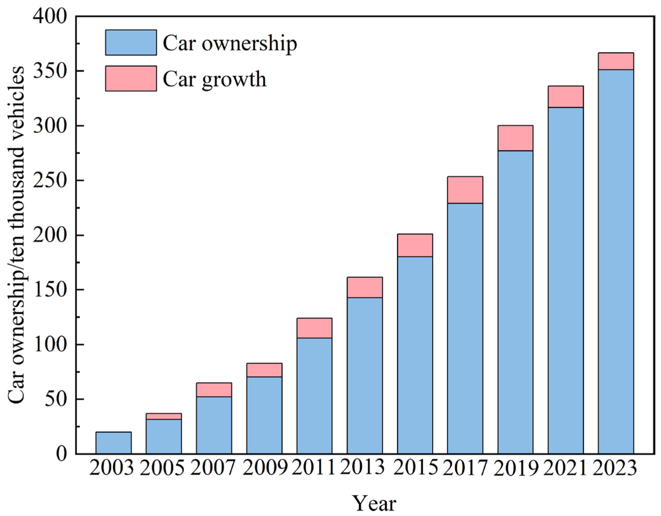
2.1. Prediction Method of Car Ownership

Firstly, we analyze the influencing factors of car ownership by employing a mixed approach that combines Kendall’s coefficient with grey correlation analysis. This “double correlation” test quantifies the correlation between each influencing factor and car ownership, enabling us to select those factors with a high degree of association as the input features for our prediction model. Subsequently, we introduce the Levy flight strategy to enhance the sparrow optimization algorithm, thereby optimizing the process for identifying the optimal smoothing factor of the GRNN. The resulting model is referred to as the LSSA-GRNN model.

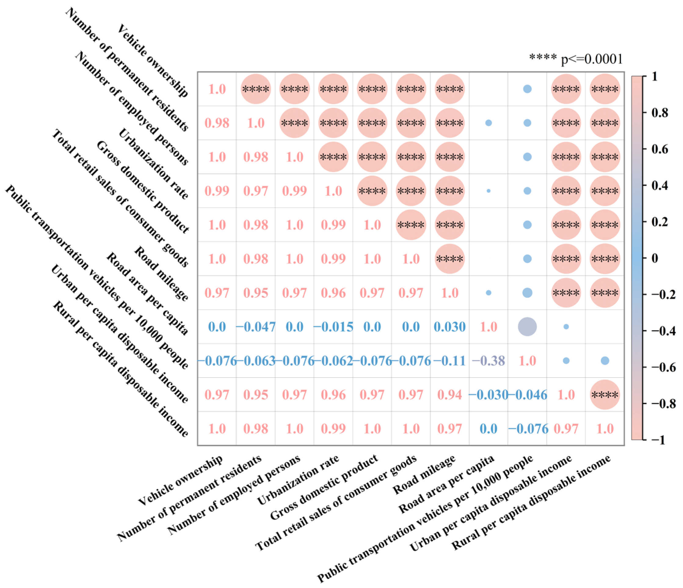
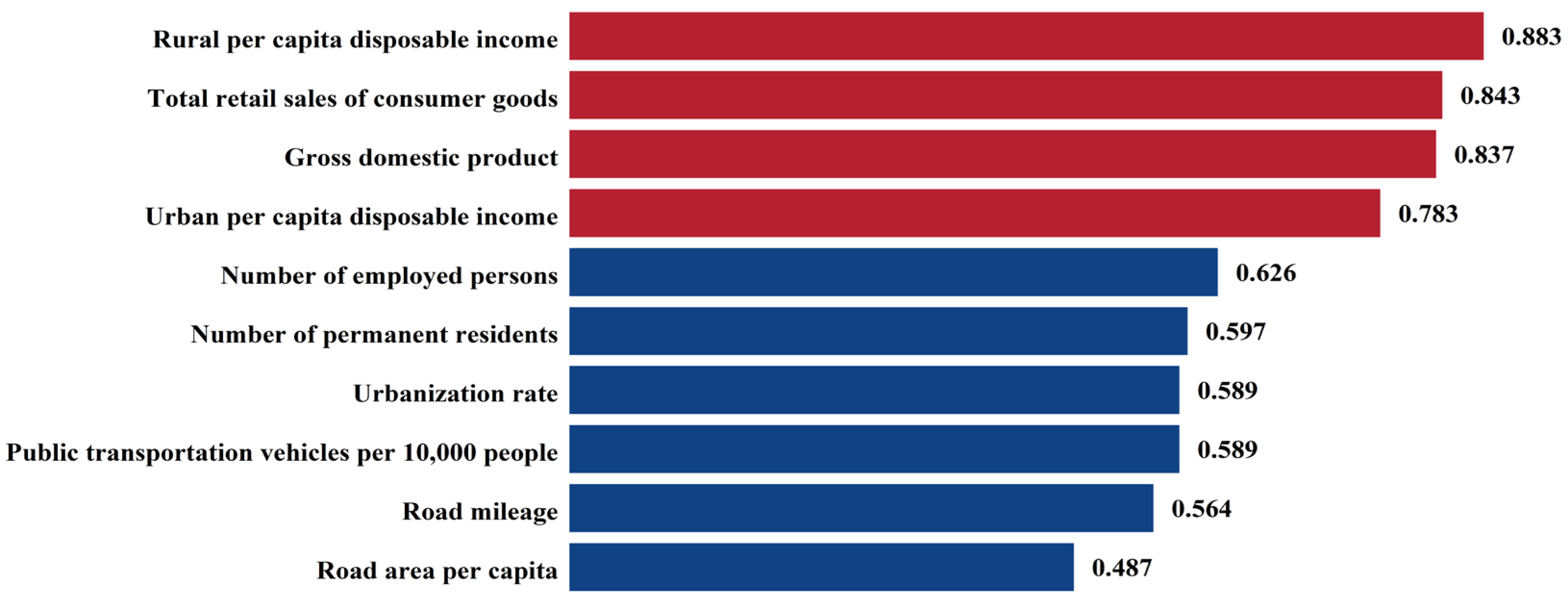
2.1.1. Influential Factor Analysis

(1)

Kendall’s correlation coefficient

Kendall’s correlation coefficient is a nonparametric method used to assess the association between two random variables by evaluating the consistency of the ordering of data pairs. Its value ranges from −1 to 1, where values closer to 1 indicate a strong positive correlation, values near −1 indicate a strong negative correlation, and values around 0 suggest a lack of significant linear relationship. Unlike the Pearson correlation coefficient, which requires data to be continuous and normally distributed and focuses on linear relationships, Kendall’s correlation is based on the concordance of ranking, making it more robust in situations where the relationships are not strictly linear yet still correlated. Furthermore, its insensitivity to outliers and extreme values enhances its suitability for analyzing the factors affecting car ownership. Consequently, this study utilizes Kendall’s correlation coefficient to rigorously evaluate and select the key determinants of car ownership.

Kendall’s correlation coefficient is calculated by assuming that $X_1,X_2,\dots ,X_n$ and $Y_1,Y_2,\dots ,Y_n$ are two sample data columns that can form a pairwise dataset with capacity n, $\left(X_i,Y_i\right)$, $i=1,2,\dots ,n$. if $\left(X_j-X_i\right)\left(Y_j-Y_i\right)>0$ then $\left(X_j,Y_j\right)$ and $\left(X_i,Y_i\right)$ are consistent with each other, if $\left(X_j-X_i\right)\left(Y_j-Y_i\right)<0$, then $\left(X_j,Y_j\right)$ and $\left(X_i,Y_i\right)$ are inconsistent with each other, and if $\left(X_j-X_i\right)\left(Y_j-Y_i\right)=0$, then $\left\{\left(X_j,Y_j\right),\left(X_i,Y_i\right)\right\}$ two data pairs are said to be a knot, which means that $\left(X_j,Y_j\right)$ and $\left(X_i,Y_i\right)$ are neither consistent nor inconsistent [25,26].

The Kendall correlation coefficient formula is as follows:

$$\tau ={\displaystyle \frac{{\displaystyle \sum _{i,j=1}^{n}sign\left[\left(X_j-X_i\right)\left(Y_j-Y_i\right)\right]}}{\sqrt{\left[\frac{1}{2}n(n-1)-n_1\right]\left[\frac{1}{2}n(n-1)-n_2\right]}}}$$

(1)

(2)

Grey correlation analysis

The essence of the grey correlation theory is to determine the closeness of the connection by determining the degree of similarity in the shape of the set of reference data columns and a number of comparative data columns, and in this way determine the degree of correlation [27]. Let $A_i$ be a factor in the system, and the sequence of behavioral characteristics of the system is (2):

$$\left\{\begin{array}{c}{A}_0=\left[a_0\left(1\right),a_0\left(2\right),a_0\left(3\right),\dots ,a_0\left(m\right)\right]\\ \begin{array}{c}{A}_1=\left[a_1\left(1\right),a_1\left(2\right),a_1\left(3\right),\dots ,a_1\left(m\right)\right]\\ \dots \\ A_i=\left[a_i\left(1\right),a_i\left(2\right),a_i\left(3\right),\dots ,a_i\left(m\right)\right]\\ \dots \\ A_i=\left[a_i\left(1\right),a_i\left(2\right),a_i\left(3\right),\dots ,a_i\left(m\right)\right]\end{array}\end{array}\right.$$

(2)

where $A_0$ is the reference data sequence and $A_1~A_n$ is the comparison data sequence.

For $\delta \in \left(0,1\right)$, let the correlation coefficient $\zeta \left(a_0\left(k\right),a_i\left(k\right)\right)$ at point K be a real number.

$$\zeta \left(a_0\left(k\right),a_i\left(k\right)\right)={\displaystyle \frac{{\min }_i{\min }_k\left|a_0\left(k\right)-a_i\left(k\right)\right|+\delta {\max }_i{\max }_k\left|a_0\left(k\right)-a_i\left(k\right)\right|}{\left|a_0\left(k\right)-a_i\left(k\right)\right|+\delta {\max }_i{\max }_k\left|a_0\left(k\right)-a_i\left(k\right)\right|}}$$

(3)

$$\lambda \left(a_0,a_i\right)={\displaystyle \frac{1}{n}}{\displaystyle \sum _{k=1}^m\zeta \left(a_0\left(k\right),a_i\left(k\right)\right)}$$

(4)

• where $k=1,2,\dots ,m;i=1,2,\dots ,n$, $\delta$ are the discriminant coefficients.

  (1)

  Normality: When condition $\lambda \left(A_0,A_i\right)=1$ equals $0<\lambda \left(A_0,A_i\right)\le 1$ and, if it equals $\lambda \left(A_0,A_i\right)=1$, then condition $A_0=A_i$ must also be met.

  (2)

  Proximity: The smaller the value of condition $\left|a_0\left(k\right)-a_i\left(k\right)\right|$, the greater is the value of condition $\zeta \left(a_0\left(k\right),a_i\left(k\right)\right)$.

  (3)

  Integrity: For condition $A_i,A_j\in A=\left\{A_u\left|u=0,1,2,\dots ,n;n\ge 2\right.\right\}$, when condition $i\ne j$ is satisfied, condition $\lambda \left(A_i,A_j\right)\ne \lambda \left(A_j,A_i\right)$ must exist.

  (4)

  Even Symmetry: When condition $A_i,A_j\in A$ is present and condition $\lambda \left(A_i,A_j\right)=\lambda \left(A_j,A_i\right)$ is met, symmetric pairwise relationships hold.

These four criteria are collectively known as the four axioms of grey relational analysis. They indicate that no two data series within the system can be entirely unrelated. Proximity serves as the constraint in quantifying the grey relational degree; integrity reflects the influence of the external environment on this degree; and even symmetry ensures that, when only two data columns are compared, the grey relational factors satisfy a symmetric condition.

When $\lambda \left(a_0,a_i\right)$ satisfies the grey correlation IV axiom, it is called the grey correlation between the reference data sequence $A_0$ and the comparison data sequence $A_i$.

2.1.2. Data Preprocessing

(1)

Missing Value Processing

Given that the influencing factors of car ownership span multiple dimensions, missing data are inevitable. Failure to properly address these missing values could result in their inadvertent inclusion during model training, thereby distorting prediction outcomes. To mitigate this risk, several imputation strategies are employed. For data columns with a low proportion of missing values and a uniform distribution, mean imputation is applied to preserve data integrity without introducing substantial bias. For columns with a high proportion of missing data, interpolation techniques are utilized to estimate the missing values based on observed trends, thus maintaining the intrinsic relationships within the dataset.

(2)

Data Standardization

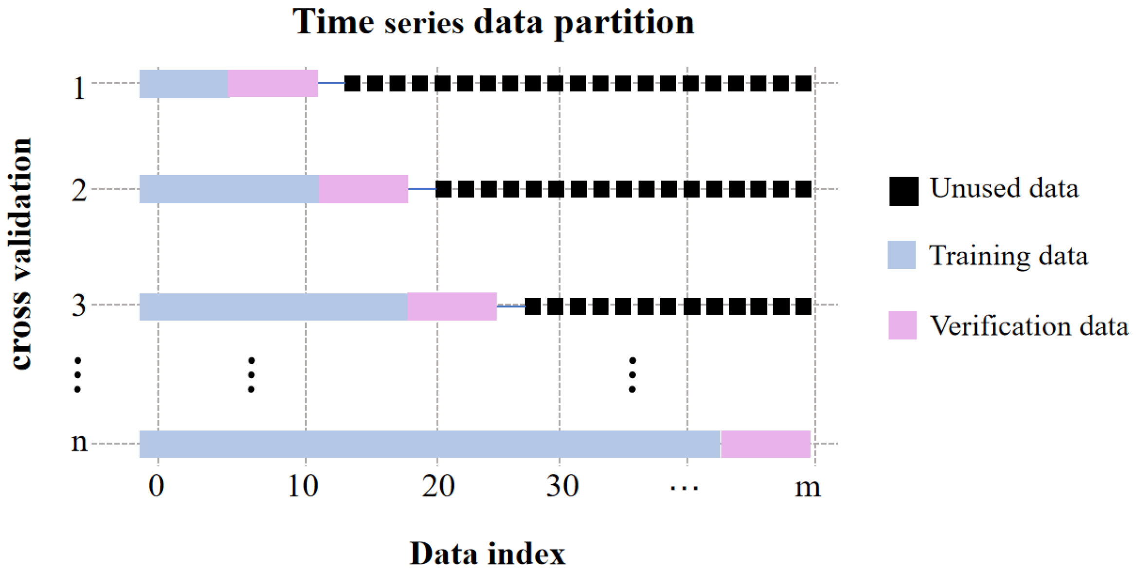
The selected influencing factors vary considerably in both dimension and range and, given that neural network algorithms are highly sensitive to the scale of input features, discrepancies in data scaling can hinder convergence during training. Therefore, it is essential to normalize the data to ensure that all input variables share a consistent scale while preserving their distributional characteristics. This study adopts the min–max normalization technique to rescale each feature to a specified range. The min–max normalization formula is expressed as

$$r\prime ={\displaystyle \frac{r-r_{\min }}{r_{\max }-r_{\min }}}$$

(5)

where $r\prime$ represents the normalized data, $r$ is the original data value, and $r_{\min }$ and $r_{\max }$ denote the minimum and maximum values of the data column, respectively.

(3)

Dataset Partitioning

A critical aspect of model evaluation is the rational partitioning of the dataset. Traditional partitioning methods—such as randomly dividing the sample data into training and testing sets (e.g., using ratios of 8:2 or 7:3)—are not appropriate for time-series data like car ownership indicators, which exhibit clear upward trends. If the temporal order is disregarded and both historical and future data are randomly allocated to the training and testing sets, the model may inadvertently incorporate future information during training, a phenomenon known as information leakage. Such leakage can artificially inflate the model’s perceived generalization performance and yield an imbalanced evaluation between training and test errors. To address these challenges, time-series cross-validation (TSCV) is employed. TSCV is specifically designed for sequential data, ensuring that the model is trained solely on historical observations. As illustrated in Figure 2, the time series is segmented into k consecutive blocks. With the exception of the first block, which can only serve as a training set, each subsequent block is initially designated as test data; subsequently, the training set is progressively expanded by incorporating preceding blocks. This approach enhances the model’s ability to learn from historical trends and ultimately improves prediction accuracy. Unlike traditional K-fold cross-validation or leave-one-out methods, TSCV maintains the inherent temporal order of the data, making it particularly suitable for time-series analyses. Consequently, TSCV is utilized in this study to partition the dataset in a manner that accurately reflects the underlying trends in car ownership data.

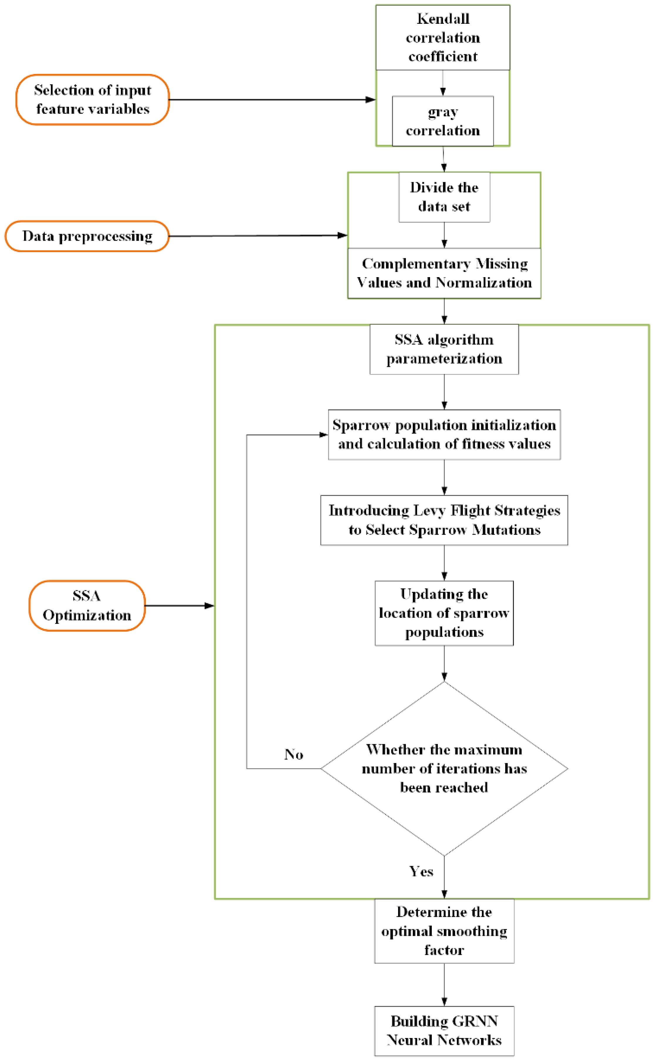
2.1.3. Implementation of the LSSA-GRNN Model

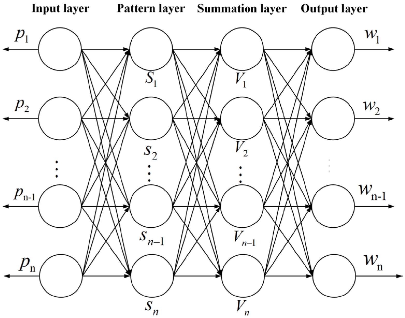
The GRNN model was selected for predicting car ownership due to its simple structure, rapid convergence, and strong adaptability when handling nonlinear and high-noise data—attributes that are particularly well-suited to the complex time-series forecasting challenge posed by the myriad economic and policy factors influencing car ownership [28]. However, traditional GRNN methods struggle to dynamically optimize the core parameter, namely the smoothing factor, to achieve its global optimum, which can adversely affect prediction accuracy. To overcome this limitation, an improved mechanism is introduced that integrates the SSA algorithm with the Levy flight strategy. Although the traditional SSA leverages the foraging and anti-predation behaviors observed in sparrow populations for efficient parameter optimization, it is often prone to becoming trapped in local optima. The incorporation of Levy’s flight strategy—characterized by its random step hybrid search mode—enhances the algorithm’s global search capabilities and helps prevent premature convergence.

(1)

GRNN model

The GRNN neural network model consists of four layers, namely, input layer, pattern layer, summation layer and output layer. $P={\left[p_1,p_2,p_3,\dots ,p_n\right]}^T$ is the input model data and $W={\left[w_1,w_2,w_3,\dots ,w_n\right]}^T$ is the output model data. The GRNN structure is shown in Figure 3.

(1) Input layer

The number of neurons in the input layer is equal to the dimension of the input data, which is transmitted directly to the pattern layer.

(2) Pattern layer

$$S_i=\exp \left[-{\displaystyle \frac{{\left(P-P_i\right)}^T\left(P-P_i\right)}{2{\mu }^2}}\right]i=1,2,3,\dots ,n$$

(6)

where $S_i$ is the output at node $i$, $P$ is the input variable, and $\mu$ is the smoothing factor.

(3) Summation layer

The summation layer has two kinds of neurons: arithmetic summation and weighted summation. The arithmetic summation formula is Equation (7), and the transfer function is Equation (8).

$${\displaystyle \sum _{i=1}^n\exp \left[-\frac{{\left(P-P_i\right)}^T\left(P-P_j\right)}{2{\mu }^2}\right]}$$

(7)

$$V_D={\displaystyle \sum _{i=1}^n{P}_i}$$

(8)

The weighted summation formula is Equation (9) and the transfer function is Equation (10).

$${\displaystyle \sum _{i=1}^n{W}_i\exp \left[-\frac{{\left(P-P_i\right)}^T\left(P-P_J\right)}{2{\mu }^2}\right]}$$

(9)

$$V_{Nj}={\displaystyle \sum _{i=1}^n{S}_{ij}{W}_i},j=1,2,3\dots ,k$$

(10)

(4) Output layer

The number of neurons in the output layer is equal to the dimension of the output variable, and the result of the output layer is obtained by dividing the outputs of the two neurons in the summation layer.

(2)

SSA algorithm

The principle of SSA algorithm [29] rule is as follows:

Suppose that there are n sparrows in the sparrow population and the expression is Equation (11).

$$B=\left[\begin{array}{c}\begin{array}{c}\begin{array}{c}\begin{array}{cccc}{b}_{1,1}& b_{1,2}& \dots & b_{1,d}\end{array}\\ \begin{array}{cccc}{b}_{2,1}& b_{2,2}& \dots & b_{2,d}\end{array}\end{array}\\ \begin{array}{cccc}\dots & \dots & \dots & \dots \end{array}\end{array}\\ \begin{array}{cccc}{b}_{n,1}& b_{n,2}& \dots & b_{n,d}\end{array}\end{array}\right]$$

(11)

$f$ denotes the fitness value of each sparrow, and the expression for the fitness value of the sparrow population is Equation (12).

$$F_b=\left[\begin{array}{c}f\left[\begin{array}{cccc}{b}_{1,1}& b_{1,2}& \dots & b_{1,d}\end{array}\right]\\ f\left[\begin{array}{cccc}{b}_{2,1}& b_{2,2}& \dots & b_{2,d}\end{array}\right]\\ ⋮\\ f\left[\begin{array}{cccc}{b}_{n,1}& b_{n,2}& \dots & b_{n,d}\end{array}\right]\end{array}\right]$$

(12)

The group position update expression is found as follows:

$$B_{i,j}^{t+1}=\left\{\begin{array}{l}{B}_{i,j}^t\cdot \exp \left(-{\displaystyle \frac{i}{\epsilon \cdot ite{r}_{\max }}}\right)\begin{array}{c}if{R}_2<ST\end{array}\\ B_{i,j}^t+E\cdot Lif{R}_2\ge ST\end{array}\right.$$

(13)

where $\mathrm{t}$ represents the number of iterations, $\epsilon$ is a random number with values ranging from 0 to 1, $ite{r}_{\max }$ denotes the maximum number of iterations, $R_2$ and $ST$ representing vigilance and safety values, respectively, Eis a set of random numbers obeying a normal distribution, and L denotes the d-matrix, whose elements are all 1.

When $R_2<ST$, it indicates that there is no predator threat in the area, and the discovery group can continue to expand the search for food.

When $R_2\ge ST$, it indicates that a predator has been detected by a vigilante and signals an alarm, at which point the location of the found group is updated to a safe area.

Follow the group position update expression as follows:

$$B_{i,j}^{t+1}=\left\{\begin{array}{l}E\cdot \exp \left({\displaystyle \frac{B_{worst}-B_{i,j}^t}{i^2}}\right)\begin{array}{cc}& i<n/2\end{array}\\ B_{best}^{t+1}+\left|B_{i,j}^t-B_{best}^{t+1}\right|\cdot H^{+}\cdot Li\le n/2\end{array}\right.$$

(14)

where $B_{worst}$ denotes the worst search position of the iterative process, $B_{best}$ denotes the best position in this iteration, $i<n/2$ indicates that the $i$ sparrow in the following group does not receive food and is hungry, and H denotes a dimensional matrix whose elements are randomly 1 or −1 and satisfy $H^{+}=H^T{\left(H{H}^T\right)}^{-1}$.

About 10% to 20% of the sparrow population are vigilantes, and the updated expression for the location of vigilantes is as follows:

$$B_{i,j}^{t+1}=\left\{\begin{array}{l}{B}_{best}^t\cdot \alpha \left|B_{i,j}^t-B_{best}^t\right|\begin{array}{cc}\begin{array}{cc}& \end{array}& \begin{array}{cc}& \begin{array}{cc}if& f_i>f_g\end{array}\end{array}\end{array}\\ B_{i,j}^t+\beta \left({\displaystyle \frac{\left|B_{i,j}^t-B_{worst}^{t+1}\right|}{\left(f_i-f_w\right)+\eta }}\right)\begin{array}{cc}& \begin{array}{cc}if& f_i=f_g\end{array}\end{array}\end{array}\right.$$

(15)

where $\alpha$ represents the step control parameter, which is a random number with mean 0 variance 1 and normally distributed, $f_i$ denotes the current fitness value of this iterative process, $f_g$ represents the best fitness value for this iterative process, and $f_w$ represents the worst fitness value for this iterative process. $\beta \in \left(-1,1\right)$ random number, $\eta$ is a fixed constant that is preventing the denominator from being zero.

When $f_i>f_g$, it means that sparrows located at the edge of the search area are vulnerable to predators and move to the center of the area to avoid the danger;

When $f_i=f_g$, it means that sparrows located in the center of the population perceive the danger and move to other safe areas to avoid the danger.

(3)

Levy Flight Strategy

In the late stage of optimization, SSA may fall into the local optimum, which makes the optimization accuracy lower, and the introduction of Levy flight strategy improves the randomness of the algorithm’s global optimization search, expands the search range, and avoids the algorithm from falling into the local optimum.

The Levy flight strategy obeys a Levy distribution [30] with the following stochastic distribution expression:

$$F_{Levy}~\phi =c^{-\rho }$$

(16)

Based on these advancements, the flow chart of the LSSA-GRNN model is presented in Figure 4.

To evaluate the performance of the LSSA-GRNN model, the root mean square error (RMSE) is employed as the error metric. RMSE quantifies the absolute error by calculating the square root of the mean of the squared differences between the predicted and observed values. A lower RMSE indicates higher predictive accuracy:

$$RMSE=\sqrt{{\displaystyle \frac{1}{n}}{\displaystyle {\sum }_{i=1}^n{(y_i-\widehat{y_i})}^2}}$$

(17)

where $n$ is the number of samples, $y_i$ is the real value, and $\widehat{y_i}$ is the predicted value.

2.2. Modeling of Carbon Emissions

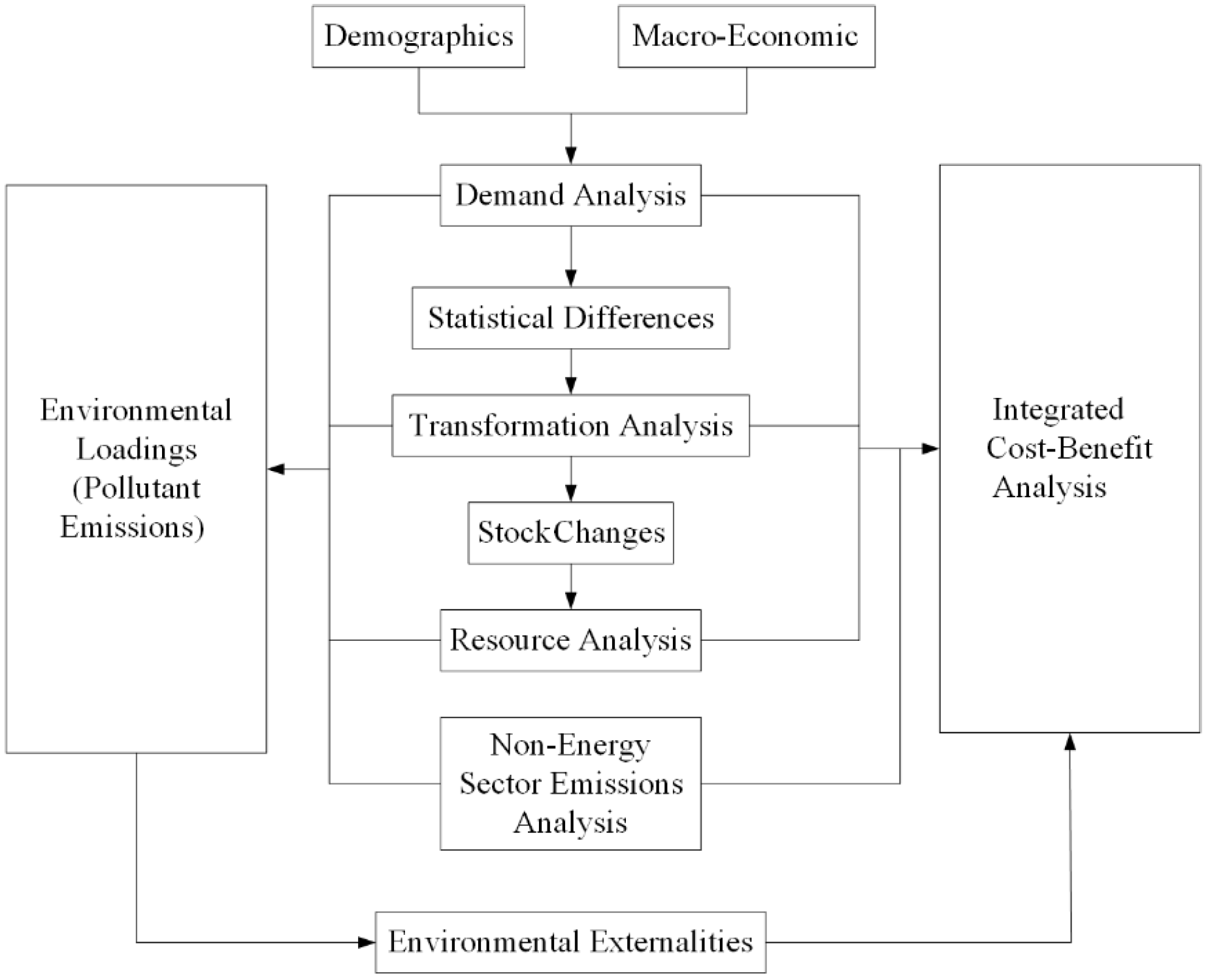
2.2.1. LEAP Model

The LEAP model is a bottom-up energy–environmental accounting tool based on scenario analysis. Developed collaboratively by the Stockholm Environment Institute (SEI) and the Boston Research Institute (BRI), it is also referred to as the Low-Carbon Emissions Analysis System. LEAP is designed to analyze and forecast energy demand, consumption, and the associated environmental impacts across diverse sectors by constructing and employing mathematical models. It facilitates the identification and quantification of emission sources for comprehensive emissions accounting.

LEAP’s versatility is demonstrated by its broad range of applications. It has been used to study pollutant management and carbon emission reduction strategies in sectors such as transportation, construction, electricity, and manufacturing. Furthermore, LEAP supports energy consumption and environmental management studies at various spatial scales—from local communities and cities to regional, national, and even global levels. Figure 5 illustrates the computational flow of the LEAP model. The modeling procedure within LEAP generally follows these steps:

(1)

Identification of the Research Domain

The LEAP framework requires clearly delineating the research domain from both spatial and temporal perspectives. Spatially, the study scope may cover national, provincial, urban, or more localized regional levels, and within the chosen area, the energy system can be analyzed in its entirety or by focusing on specific sectors. Temporally, a base year is established, and the time horizon for the scenario analysis is defined accordingly.

(2)

Development of the Data Structure

LEAP employs a hierarchical tree data structure that organizes information from the highest system level down to individual sectors, end-use technologies, energy types, and carbon dioxide emission factors. This structured approach ensures consistency and comprehensiveness in the energy–environmental analysis.

(3)

Scenario Design

Establishing well-defined scenarios is critical to the analytical rigor of the study. The parameters for the base year are calibrated to reflect current socio-economic conditions, while scenario elements are derived from relevant policy documents and the scientific literature. These scenarios incorporate factors such as demographics, economic trends, social dynamics, environmental conditions, and political contexts to simulate possible future pathways.

(4)

Results Analysis

The outcomes generated by the LEAP model are evaluated by comparing environmental impacts across different scenarios. The analysis focuses on identifying how various design measures influence sector-specific results, thereby providing insights into effective regulatory and policy measures that can drive carbon emission reductions and support sustainable energy transitions.

2.2.2. Calculation of Carbon Emissions

The formula for calculating [31] CO₂ emissions from conventional fuel vehicles is as follows:

$$VC={\displaystyle \sum _{i,j}V{N}_{i,j}\cdot E{C}_{i,j}\cdot V{M}_{i,j}\cdot E{F}_j}$$

(18)

• $VC$—Total CO₂ emissions from conventional fuel vehicles;
• $i$—Type of vehicle used for transport, e.g., car, taxi, bus, etc;
• $j$—Type of energy used for transport, e.g., petrol, diesel, natural gas, etc;
• $V{N}_{i,j}$—Number of vehicles of type i models using type j energy (units);
• $E{C}_{i,j}$—Average consumption per unit kilometer for the i model of vehicle using the j energy source (L/100 km, m³/100 km);
• $V{M}_{i,j}$—Average annual mileage of the i model using the j energy source (km);
• $E{F}_j$—Carbon dioxide emission factor of the j energy source.

Electric vehicles and traditional fuel vehicles [31] are different, the car running process will not directly produce carbon emissions, but the consumption of electricity in the process of generating carbon emissions cannot be ignored, and in the process of power transmission and charging process caused by the loss will affect the carbon emissions of electric vehicles. Electric vehicle carbon emissions are as shown in Equation (16).

$$V{C}_e={\displaystyle \sum _i\frac{V{N}_{\mathrm{i},\mathrm{e}}\cdot E{C}_{i,e}\cdot V{M}_{i,e}\cdot E{F}_s}{{\eta }_1\cdot {\eta }_2}}$$

(19)

• $V{C}_e$—CO₂ emissions of electric vehicles.
• $V{N}_{\mathrm{i},\mathrm{e}}$—The number of electric vehicles of the i type (units).
• $E{C}_{i,e}$—Average consumption per unit kilometer of type i electric vehicles (kw·h/100 km).
• $V{M}_{i,e}$—Average annual mileage of the i electric vehicle (km).
• $E{F}_s$—Carbon dioxide emission factor of electric power.
• ${\eta }_1$—Efficiency of electricity transportation.
• ${\eta }_2$—Charging efficiency of electric vehicles.

3. Construction of the Model

3.1. Car Ownership LSSA-GRNN Forecasting Model

3.1.1. Analysis of Influencing Factors

When forecasting car ownership in Ningbo, we selected 10 indicators from the dimensions of socio-economics, population size, road resources, and public transportation. Considering data availability, we compiled 20 years of data (2003–2022) for Ningbo, which were obtained from the Ningbo Municipal Bureau of Statistics. Using Origin 2025 data analysis software, we performed a Kendall correlation coefficient analysis on these 10 indicators relative to car ownership, as illustrated in Figure 6. The results indicate that, among the 10 selected indicators, per capita road area and the number of public transportation vehicles per 10,000 people exhibit low Kendall correlation coefficient values, suggesting a weak significance and minimal correlation with car ownership.

To further assess the driving effects of these influencing factors and determine the degree of correlation with car ownership, grey correlation analysis was conducted using SPSSPRO software (web version). The calculation results are shown in Figure 7. Based on these results, the indicators, ranked in descending order of correlation with automobile ownership, are as follows: rural per capita disposable income, total retail sales of social consumer goods, gross regional product, urban per capita disposable income, number of employed people, total resident population, number of public transportation vehicles per 10,000 people, urbanization rate, highway mileage, and per capita road area. In accordance with the factor selection principle described in Section 2, the four indicators finally selected as the input variables for the car ownership prediction model are rural per capita disposable income, total retail sales of consumer goods, gross regional product, and urban per capita disposable income.

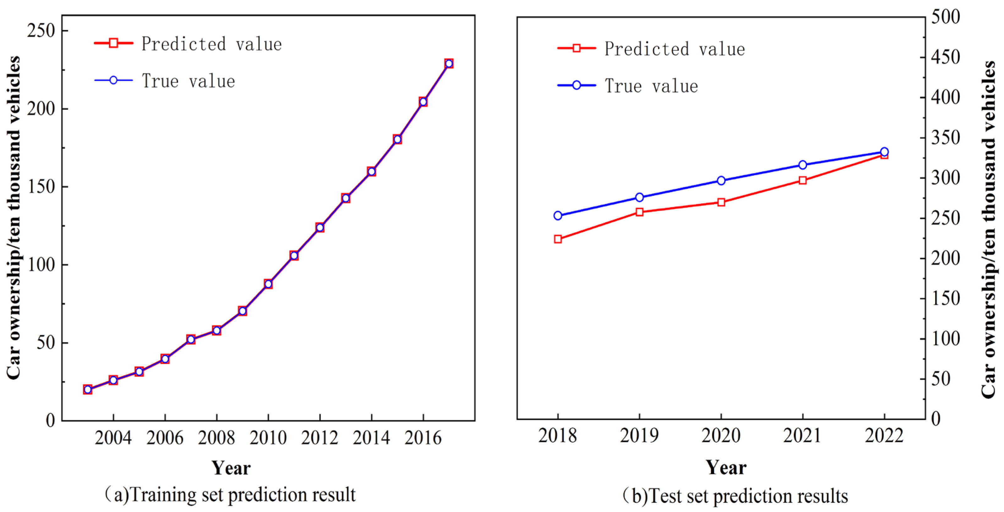
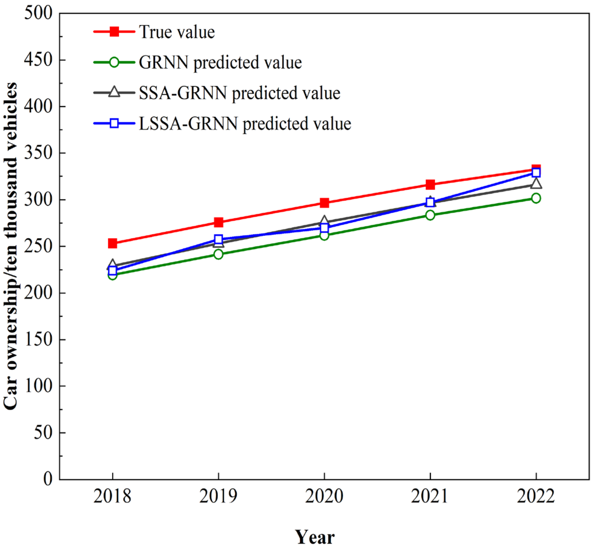
3.1.2. Analysis of Projected Results

Prior to predicting car ownership in Ningbo, data preprocessing methods described in Section 2 were applied to address missing values and to normalize the data, thereby eliminating the influence of different data dimensions on the prediction results. Time series cross-validation (TSCV) was used to partition the dataset, with 2003–2017 designated as the initial training set and 2018 set as the first test year. In each subsequent round, the training set is incrementally expanded by adding data from one previous year, and the test set is pushed backward one year so that the test period always spans two consecutive years. For every round of training and prediction, the predicted car ownership in the test set is recorded using various error metrics. To mitigate the influence of model prediction fluctuations on the evaluation, each round is repeated 15 times, and the average of the prediction results is taken as the final model output, thereby enhancing the stability and reliability of the results.

Figure 8 illustrates the prediction results of the model. Comparison of the training set and test set results shows that the LSSA-GRNN model provides an excellent fit to the historical data. During the training phase, the model’s predictions almost exactly coincide with the actual values, with the overall trend being consistent and the error very small. This outcome indicates that the model has a strong learning capacity for historical samples and can effectively capture the nonlinear relationship between the input features and car ownership. In the testing phase, although some deviations between the predicted and actual values are observed, the overall trend remains the same with only minor fluctuations. For individual years, some slight underestimation or overestimation occurs; however, these errors fall within a reasonable range and no systematic bias is detected.

To further validate the performance of the LSSA-GRNN model in predicting urban car ownership, its results were compared with those of a traditional GRNN model and a SSA-GRNN model. The prediction outcomes are summarized in

Table 1. Multi-model prediction results.

Year	Ture Value	GRNN Predicted Value	SSA-GRNN Predicted Value	LSSA-GRNN Predicted Value
2018	253.83	219.26	229.01	223.98
2019	277.02	241.53	253.09	257.60
2020	297.14	261.73	275.81	269.76
2021	316.58	283.30	296.72	297.08
2022	335.71	301.63	316.23	328.86

and illustrated in Figure 9. Table 1 reveals that the GRNN model consistently underestimates the forecast values across different years—most notably, in 2018, where the prediction was only 2,192,600 vehicles compared with the actual 2,538,300 vehicles—indicating that this model is prone to a forecast lag when handling time-series data. Although the SSA-GRNN model improved prediction accuracy, it still tended to yield conservative estimates overall. In contrast, the predictions generated by the LSSA-GRNN model exhibit high consistency with the actual values for each year. As shown in Figure 8, the forecast curve produced by the LSSA-GRNN model closely mirrors the observed trend, with a smoother and more reasonable trajectory and minimal numerical error.

The RMSE values for the models are reported in

Table 2. Multi-model RMSE results.

Year	Ture Value	RMSE of GRNN	RMSE of SSA-GRNN	RMSE of LSSA-GRNN
2018	253.83	0.1337	0.9512	0.0645
2019	277.02	0.1243	0.08238	0.0616
2020	297.14	0.1146	0.0704	0.0438
2021	316.58	0.1041	0.0617	0.0396
2022	335.71	0.0928	0.0489	0.0287

. The GRNN model exhibits an unusually high RMSE in 2022, suggesting instability in response to recent data changes. Although the SSA-GRNN model remains stable from 2020 to 2022, its error levels remain relatively high. Conversely, the LSSA-GRNN model consistently produces low RMSE values across all years, showing a decreasing trend from 0.0645 in 2018 to 0.0287 in 2022. These findings demonstrate that the LSSA-GRNN model outperforms both the GRNN and SSA-GRNN models in terms of stability and generalization ability when handling long-term time-series prediction tasks.

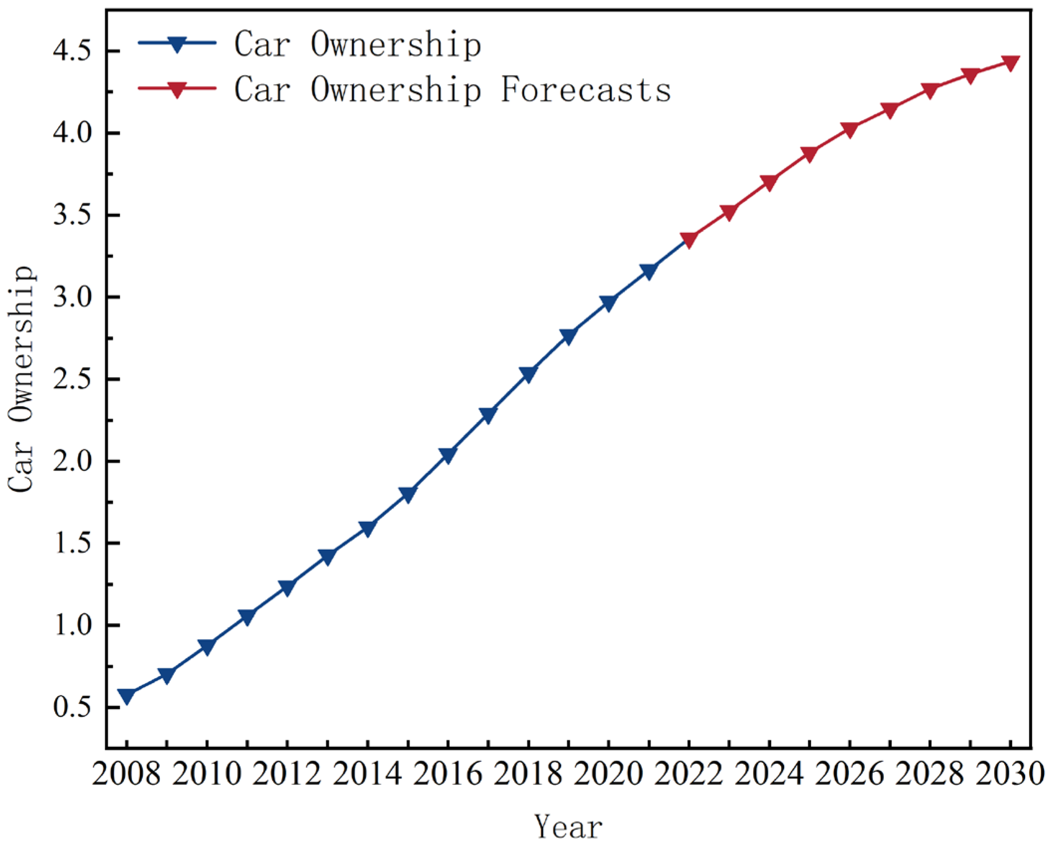
3.1.3. Projections for Future Years

The SARIMA time-series model was employed to forecast four key influencing factors from 2023 to 2030, and the predicted values are presented in

Table 3. Prediction results for the 4 input characterization variables.

Year	Urban per Capita Disposable Income/Yuan	Rural per Capita Disposable Income/Yuan	Total Retail Sales of Consumer Goods/Billion Yuan	GDP/Billion Yuan
2023	81,759.20	48,753.97	5347.27	17,068.20
2024	86,758.19	53,001.04	5768.46	18,700.41
2025	92,179.26	57,644.43	6228.92	20,454.93
2026	97,921.53	62,721.30	6727.62	22,386.43
2027	104,028.69	68,266.77	7266.56	24,500.67
2028	110,517.64	74,320.96	7848.69	26,814.84
2029	117,412.62	80,928.31	8474.03	29,347.67
2030	124,738.43	88,137.71	9152.03	32,119.80

. These four factors are then used as input variables for the car ownership prediction model. The trained LSSA-GRNN model forecasts car ownership in Ningbo for the period 2023–2030, and the results, shown in Figure 10, indicate that, while car ownership in Ningbo will continue to increase, its growth rate is expected to slow compared with previous years.

3.2. Urban Transport Carbon Emission Modeling

3.2.1. Structural Division of Carbon Emissions

Due to anticipated data fluctuations resulting from the implementation of time-limited area restriction policies for various truck models in Ningbo, this study focuses solely on the passenger transport system. Drawing on the LEAP model framework, the urban transport carbon emission model is structured into four layers, as detailed in

Table 4. Segmentation of different vehicle carbon emission structures for urban transportation.

System	Subsectors	Terminal Equipment	Consumption of Energy
Passenger transport	Individual transport	Microbus	Petrol
			Electricity
	Public transport	Medium and large buses	Diesel
			Electricity
		Public Trams	Natural Gas
			Diesel
			Electricity
		Taxi	Petrol
			Natural gas
			Electricity
		Railway	Electricity

.

In the first layer, the passenger transport system is divided into two subsectors: individual transport and public transport. Terminal equipment is classified according to the China Motor Vehicle Classification Standard; within the passenger transport category, vehicles are further subdivided into micro-small buses, medium-sized and large buses, taxis, and buses. The model distinguishes fuel types—including petrol, diesel, natural gas, and electricity—based on the energy source utilized by the terminal equipment.

3.2.2. Baseline Parameter Setting

For the base year (2022), the car ownership structure in Ningbo is dominated by traditional fuel vehicles, despite a robust growth in new energy vehicles. Specifically, gasoline-powered vehicles account for approximately 94.5% of micro-small buses, with electric vehicles representing about 5.5%. In contrast, public buses in Ningbo have responded positively to national initiatives promoting new energy public transport, with electric buses comprising roughly 73% of the fleet, natural gas buses around 11%, and diesel buses about 16%. Among taxis, natural gas vehicles account for approximately 76%, with electric vehicles and gasoline vehicles representing about 22% and 2%, respectively. The 100 km energy consumption data for each vehicle model in Ningbo are obtained from the China Automotive Energy Consumption data provided by the Ministry of Industry and Information Technology (MIIT), and the average annual mileage is set according to statistics from the Ningbo Transport Bureau, in conjunction with national transport sector statistics and the ‘Provisions on Compulsory Motor Vehicle End-of-Life Standards’. Benchmark parameters and required data for the modeling are shown in

Table 5. Sectoral parameterization of automotive carbon emissions in the base year.

Terminal Equipment	Ownership (Vehicles)	Average Annual Mileage (km)	Energy Consumption	Fuel Share (%)	Energy Consumption per 100 km
Microbus	2,891,345	12,222.88	Petrol	94.5	8.82 L/100 km
			Electricity	5.5	15.1 kw·h/100 km
Medium and large buses	35,546	43,333	Diesel	100	20 L/100 km
			Electricity	0	64.5 kw·h/100 km
Public Trams	9063	52,118.64	Natural Gas	11	33.18 m3/100 km
			Diesel	16	30.2 L/100 km
			Electricity	73	64.5 kw·h/100 km
Taxi	6135	79,198.43	Petrol	76	16.45 m3/100 km
			Natural gas	2	8.62 L/100 km
			Electricity	22	15.1 kw·h/100 km
Railway	1056	23,287	Electricity	100	184.33 kw·h/100 km

.

Carbon dioxide emission factor calculation variables for gasoline, diesel, and natural gas are derived from the ‘China Energy Statistics Yearbook 2022’ and the ‘Guidelines for the Preparation of Provincial Greenhouse Gas Inventories (Trial)’. In addition, carbon dioxide emission factors for electric vehicles and power generation structure are obtained from the ‘Announcement on the Publication of Electricity CO₂ Emission Factors in 2022’, while the carbon dioxide emission factor for electric power is based on the average provincial CO₂ emission factor for electric power in Zhejiang Province for 2022 (0.5153 kg CO₂/kW·h). The corresponding carbon dioxide emission factor parameters are detailed in

Table 6. Carbon dioxide emission factors for different fuel types with associated parameters.

Fuel Type	Carbon Content per Unit t C/GJ	Carbon Oxidation Rate%	Carbon Dioxide Emission Factor Kg CO2/GJ or kg CO2/kW·h
Petrol	0.0189	98	67.92 kg CO2/GJ
Diesel	0.0202	98	72.64 kg CO2/GJ
Natural Gas	0.0153	99	55.56 kg CO2/GJ
Electricity	/	/	0.5153 kg CO2/kW·h

.

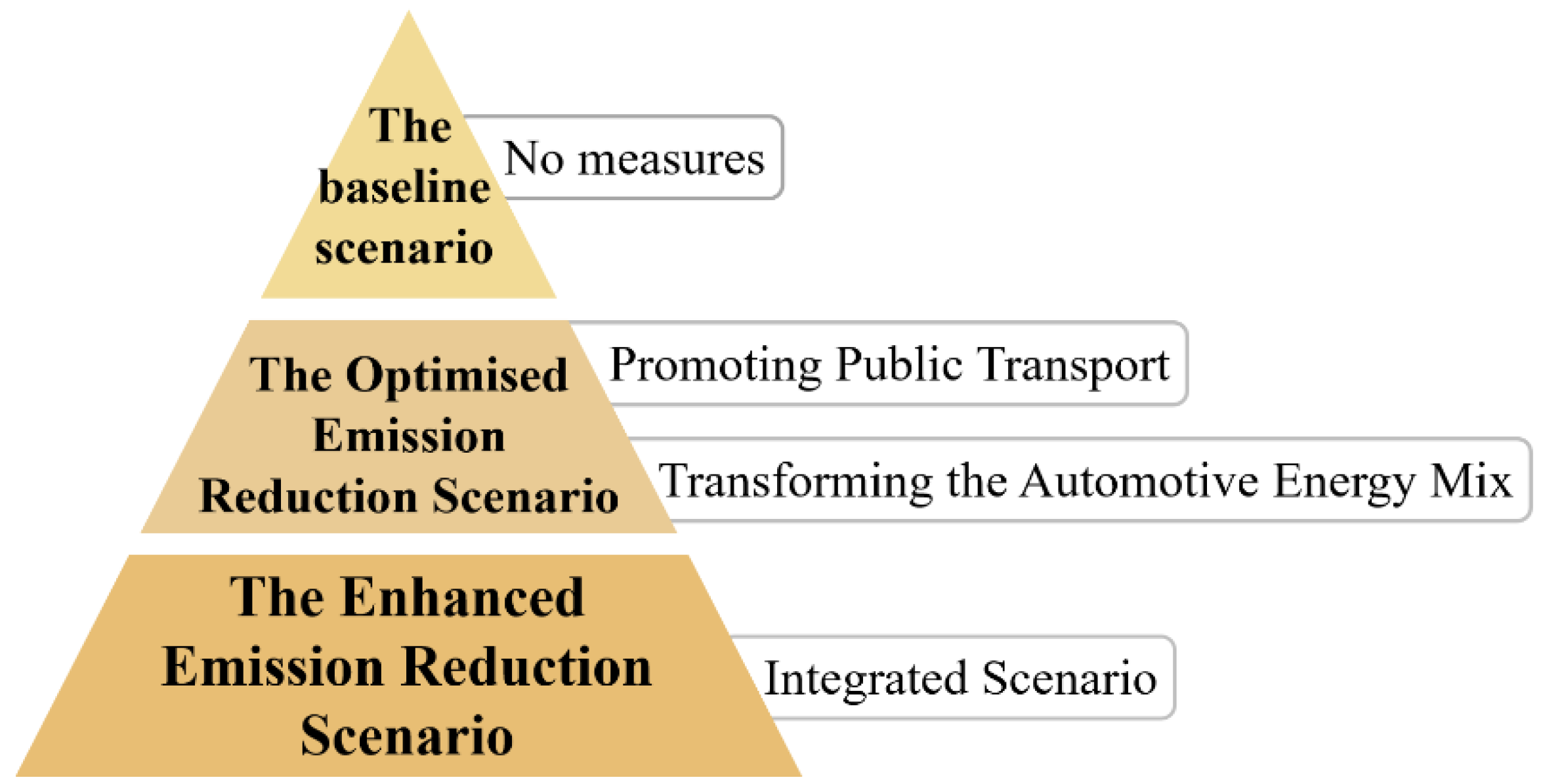
3.2.3. Scenario Design

To achieve carbon emission reduction targets in the transport sector, the Ningbo municipal government has implemented a range of measures, including the promotion of new energy vehicles, the accelerated retirement of older vehicles, the enhancement of vehicle emission standards, the encouragement of public transport, and the optimization of the overall transport structure. Building upon these initiatives, this study develops a three-tier scenario framework to assess urban transport carbon emissions under varying policy and technological conditions. As illustrated in Figure 11, the framework comprises a baseline scenario (lower tier), an optimized emission reduction scenario (middle tier) featuring multiple single-measure sub-scenarios, and an enhanced emission reduction scenario (top tier) that combines comprehensive measures of varying intensities.

The Baseline Scenario serves as a reference case, assuming that car ownership and usage patterns continue along historical trajectories without additional policy intervention. Under this scenario, key parameters—such as vehicle type composition, fleet mix, average annual mileage, and energy intensity—remain unchanged from the base year (2022).

The Optimized Emission Reduction Scenario builds upon the baseline scenario by incorporating targeted sub-scenarios that adjust energy intensity, mileage, and vehicle ownership structure. On one hand, the scenario promotes the development of public transportation, encourages green travel behaviors among residents, increases the modal share of public transit, and reduces the mileage of private vehicles, all of which contribute to emission reductions. On the other hand, since traditional fuel vehicles generate significantly higher carbon emissions than new energy vehicles, the scenario also emphasizes the substitution of conventional vehicles with electric ones and improvements in energy efficiency across all vehicle types. The sub-scenarios are designed as follows:

➀

Promoting Public Transport Ⅰ: The average annual mileage of individual transport is reduced by 1% per year relative to the base year, while the average mileage of public transport increases by 1% annually.

➁

Promoting Public Transport Ⅱ: The average annual mileage of individual transport is reduced by 2% per year relative to the base year, with a corresponding 2% annual increase in the average mileage of public transport.

➂

Transforming the Automotive Energy Mix Ⅰ: By 2025, all new vehicle sales in Ningbo will be purely electric, and all public transport vehicles will transition to clean or new energy sources. By 2030, the number of new energy vehicles will reach 800,000, with 100% electrification of public transport vehicles. Additionally, the energy intensity of each vehicle type will be reduced by 1% annually from the base year level, in alignment with national targets for automotive energy efficiency.

➃

Transforming the Automotive Energy Mix Ⅱ: By 2025, new energy vehicles will constitute 20% of Ningbo’s total vehicle stock, with complete electrification of public transport. From the base year, energy intensity for all non-electric fuels will be reduced by 1% annually, while the energy intensity of electricity will decline by 1.5% annually. By 2030, all newly sold vehicles will be fully electric.

The Enhanced Emission Reduction Scenario integrates both public transport promotion and vehicle energy mix transformation measures from the optimized scenario. It proposes four composite sub-scenarios in which Ningbo not only prioritizes the expansion of public transport and its modal share but also accelerates the adoption of new energy vehicles and improves the energy efficiency of fuel-powered vehicles. These integrated measures aim to facilitate low-carbon travel within the individual transport sector. The detailed design of the integrated sub-scenarios is provided in

Table 7. Comprehensive scenario design table.

Scenario Name	Intensity of Measures to Promote Public Transport	Intensity of Measures to Change the Energy Mix of Vehicles
Integrated Scenario Ⅰ	Promoting Public Transport Ⅰ	Transforming the Automotive Energy Mix Ⅰ
Integrated Scenario Ⅱ	Promoting Public Transport Ⅱ	Transforming the Automotive Energy Mix Ⅰ
Integrated Scenario III	Promoting Public Transport Ⅰ	Transforming the Automotive Energy Mix Ⅱ
Integrated Scenario Ⅳ	Promoting Public Transport Ⅱ	Transforming the Automotive Energy Mix Ⅱ

.

4. Results

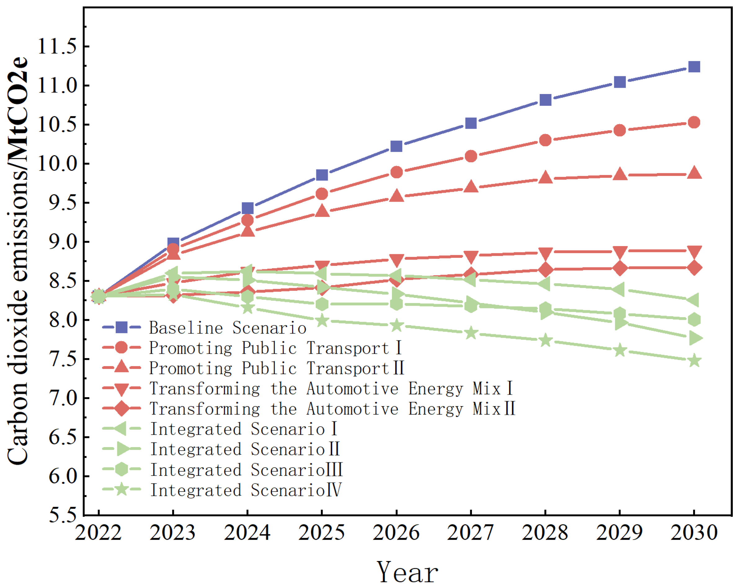
4.1. Analysis of Carbon Emission Results by Scenario

Figure 12 presents the total CO₂ emissions for each scenario. Under the baseline and optimized low-carbon scenarios, none of the sub-scenarios achieve a carbon peak by 2030; however, the optimized low-carbon scenario exhibits a marked reduction in overall emissions and a gradual decline in the annual growth rate. In contrast, all sub-scenarios within the enhanced low-carbon scenario manage to reach peak carbon by 2025.

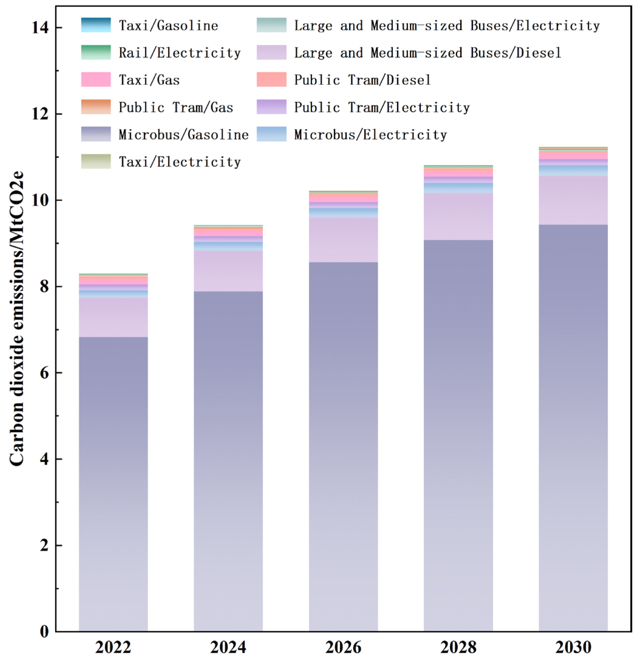
4.1.1. Baseline Scenario

In the Baseline Scenario (see Figure 13), no specific carbon reduction measures are implemented, and as a result, CO₂ emissions continuously rise in tandem with increasing car ownership and transportation demand in Ningbo. Initially, the increase in emissions is relatively gradual; however, as economic development and urbanization accelerate, the growth rate of emissions notably increases in the middle to later stages. By 2030, total emissions reach 11,239,100 tons—a 35.38% increase relative to 2020. Throughout this period, passenger vehicles dominate emissions, with gasoline minibuses accounting for approximately 84% of the total. Although bus emissions also increase, their growth rate is slower, and their proportional contribution gradually declines. Large and medium-sized buses display steady growth, while taxis and rail transit, despite having lower overall emissions, exhibit an upward trend over the long term.

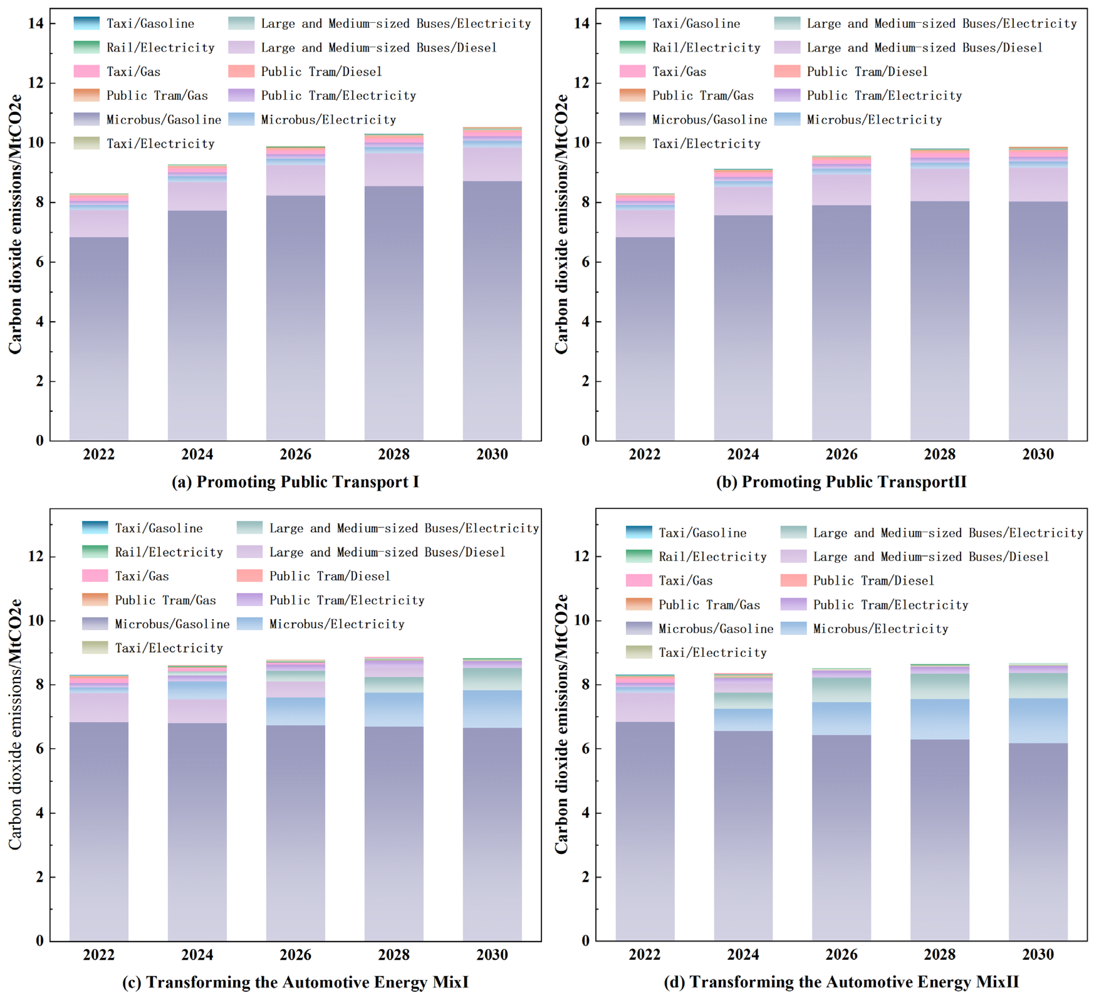
4.1.2. Optimization of Low-Carbon Scenarios

Figure 14 illustrates the emissions under the optimized low-carbon scenario, which comprises four sub-scenarios with varying intensities of emission reduction measures. Overall, the optimized scenario successfully controls total carbon emissions, showing a significant downward trend compared to the baseline—particularly in the medium and later stages. By 2030, emissions under the sub-scenarios for “Promoting Public Transport I”, “Promoting Public Transport II”, “Transforming Automobile Energy Structure I”, and “Transforming Automobile Energy Structure II” are 10,527,300 tons, 9,867,400 tons, 8,881,300 tons, and 8,671,500 tons, respectively. While both types of measures contribute to emission reductions, the scenarios based on transforming the automotive energy structure are notably more effective, with some sub-scenarios even showing a negative growth trend in emissions (e.g., a marked decline in emissions from gasoline minibuses). In contrast, although the public transport promotion scenarios reduce emissions relative to the baseline, their annual average emissions remain higher than those observed in the energy structure transformation scenarios.

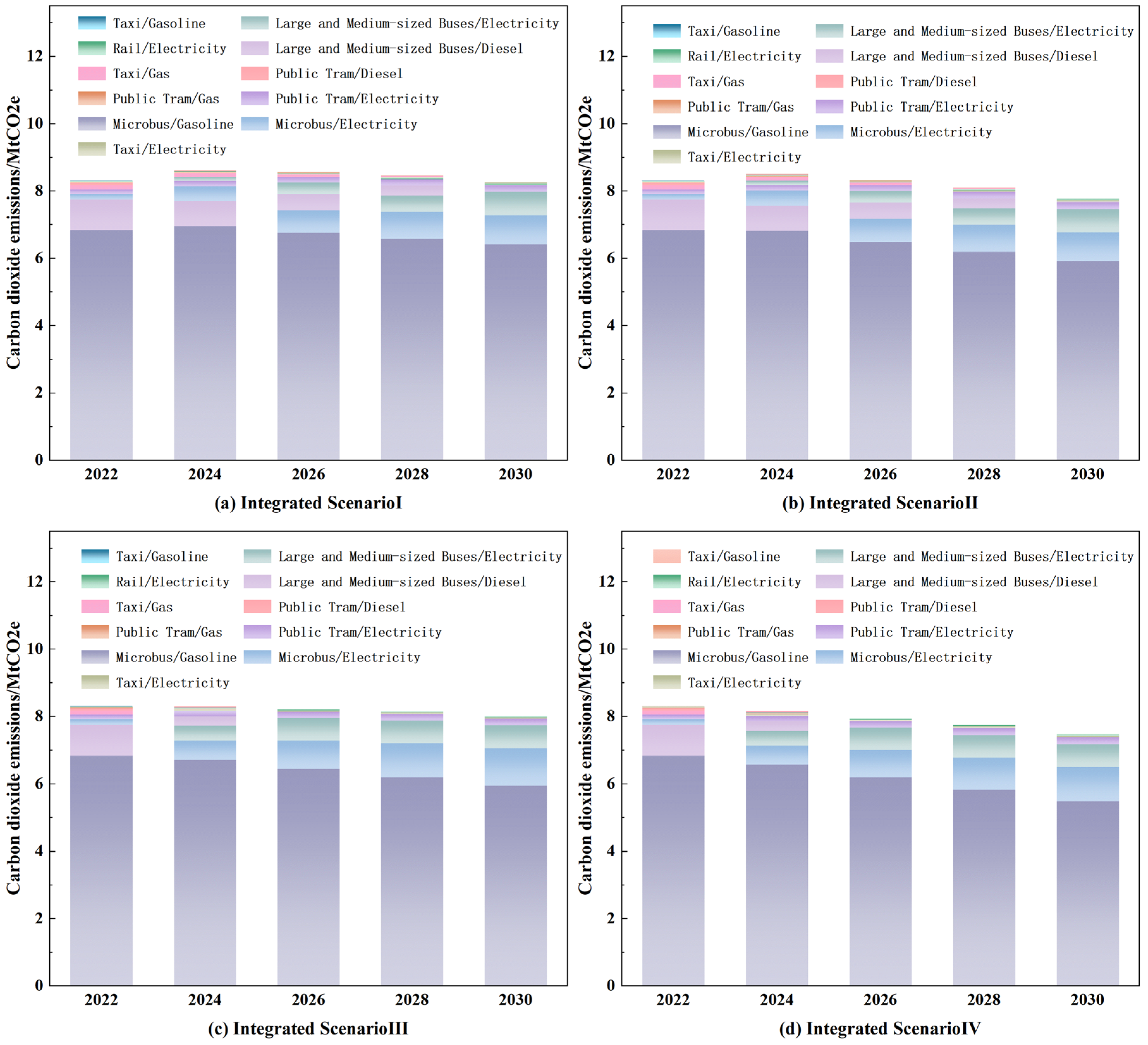
4.1.3. Enhanced Low-Carbon Scenarios

Figure 15 shows the emissions for the Enhanced Low-Carbon Scenario, which integrates both public transport improvements and automotive energy structure transformations. This comprehensive approach demonstrates the most pronounced effect in controlling carbon emissions. Overall, emissions initially decline, and while Comprehensive Scenarios I and II experience a period of slow increase followed by a year-on-year decline, Comprehensive Scenarios III and IV exhibit a consistent annual decrease. By 2030, the total emissions for Comprehensive Scenarios I, II, III, and IV are 8,258,000 tons, 7,771,400 tons, 8,008,000 tons, and 7,480,900 tons, respectively—representing reductions of up to 26.52% and an absolute decrease of 308,900 tons compared to the baseline.

Examining individual transport modes, passenger vehicles—traditionally a major contributor to carbon emissions—show significant reductions under strengthened low-carbon measures. The aggressive promotion of new energy vehicles, tighter control over private vehicle travel intensity, and increased electrification have considerably lowered emissions from private cars. Meanwhile, the bus subsystem experiences substantial emission reductions, with public transport buses nearing zero emissions due to widespread adoption of clean energy. Emissions from large and medium-sized buses stabilize and slightly decline over time as energy efficiency improves and new energy buses gradually replace older, fuel-based models. Although taxi emissions are relatively small, they also show a slight downward trend driven by the uptake of new energy vehicles and greater public transport adoption. Conversely, as residents increasingly rely on rail transit, its emissions exhibit an upward trend, reflecting the comprehensive implementation of low-carbon policies across the transportation system.

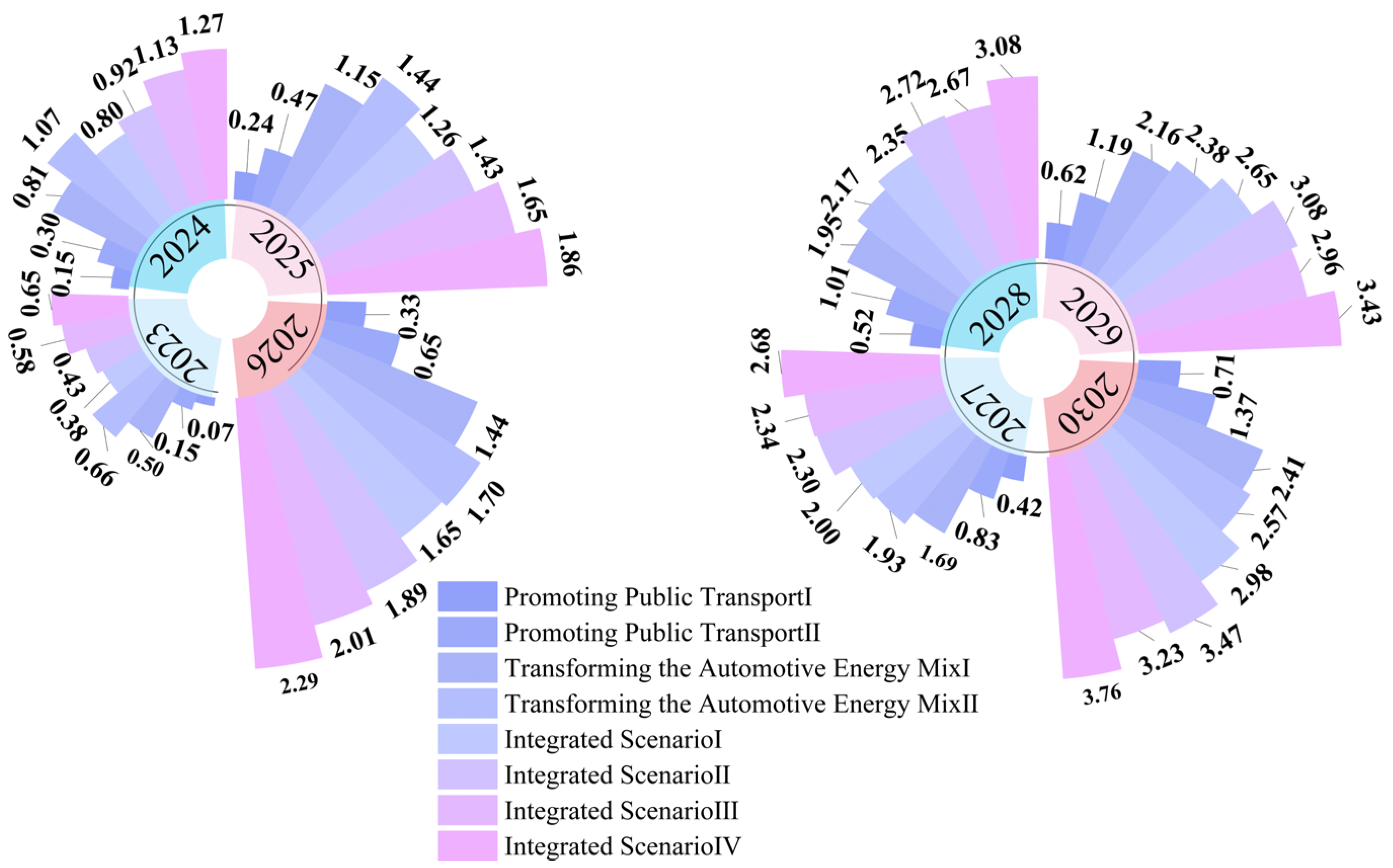
4.2. Sub-Scenario Carbon Reduction Potential Analysis

Figure 16 compares the carbon reduction capacities of the various scenarios. In the optimized low-carbon scenario, the sub-scenarios that focus solely on public transport promotion achieve moderate annual carbon reductions of 30,600 tons and 59,700 tons by 2030. In contrast, scenarios that emphasize transforming the automotive energy structure yield an annual carbon reduction of approximately 25,000 tons by 2030. The enhanced carbon reduction scenario, which combines these measures, results in a significantly greater reduction effect. For example, Comprehensive Scenario I, which integrates “Promoting Public Transport I” with “Transforming Automobile Energy Structure I”, achieves a fivefold increase in carbon reduction compared to public transport measures alone, while Comprehensive Scenario II contributes to a 30% reduction in total emissions by 2030. Comprehensive Scenario IV, which simultaneously implements multiple aggressive measures—including accelerated vehicle upgrading, increased electrification, and promotion of green travel—achieves an annual reduction of approximately 38,000 tons.

In summary, the integrated approaches represented by Comprehensive Scenarios IV and II offer the greatest potential for carbon emission reduction, followed by Comprehensive Scenarios III and I, and then the standalone automotive energy structure transformation scenarios. Although public transport promotion has a relatively smaller quantitative impact, it serves as a crucial auxiliary measure. Consequently, future strategies in Ningbo should emphasize technological innovation to reduce unit energy consumption, enforce stringent vehicle emission standards, increase public transport frequency and attractiveness, and promote a shift from private to new energy transportation. These concerted efforts will help transform the urban transportation system toward a more sustainable, low-carbon future.

5. Conclusions

By analyzing the carbon dioxide emission factors specific to Ningbo, we calculated the CO₂ emissions in the passenger transport sector from 2022 to 2030, using 2022 as the base year and incorporating forecast retention data under multiple scenarios. The calculation results indicate that

(1)

Under the Baseline Scenario, Ningbo will not achieve carbon peaking in the transport sector by 2030, with annual emissions rising to 11,239,100 tonnes.

(2)

Under the Optimized Low-Carbon Scenario, the implementation of targeted carbon reduction measures leads to reduced emissions. Within this scenario, the sub-scenario that promotes public transport exhibits a lower potential for reducing carbon emissions, reaching 9,867,400 tonnes in 2030 and yielding an annual reduction of up to 13,700 tonnes. In contrast, the sub-scenario focusing on transforming the automotive energy structure shows stronger emission reduction potential, with 2030 emissions estimated at no more than 8,671,500 tonnes and achieving a reduction of 14,400 tonnes in 2025. Despite its higher potential, the energy structure transformation measures face challenges related to the widespread adoption of new energy vehicles and enhancing the performance of conventional vehicles. Notably, none of the scenarios achieve carbon peaking by 2030.

(3)

Under the Enhanced Low-Carbon Scenario, which integrates and intensifies measures from the optimized low-carbon scenario, the overall emission reduction effect is more pronounced. In this integrated scenario, the maximum total carbon emissions in 2030 are projected to be 8,258,000 tonnes, with annual emission reductions ranging from 29,800 to 37,600 tonnes, signifying a significant improvement over the other scenarios.

It is noteworthy that the car ownership prediction model was validated against Ningbo’s statistical data; the predicted trends generally align with observed patterns, and the conclusions appear to be fundamentally sound. However, the limited sample size constrains the model’s generalization ability. With richer data and further model refinements, prediction accuracy and the precision of subsequent analyses could be significantly enhanced. Moreover, due to data limitations and concerns about related traffic policies, our analysis focused solely on the passenger transport system; the vehicle data for Ningbo’s freight system were unavailable, and its contribution to overall carbon emissions was not evaluated. This limitation may lead to some discrepancies between our calculated emissions and the actual total urban traffic emissions. Future research should incorporate a comprehensive analysis that includes the freight system to more accurately evaluate the full potential for carbon emission reduction in Ningbo’s urban transportation.

References

1. Dargay, J.M.; Vythoulkas, P.C. Estimation of a dynamic car ownership model: A pseudo-panel approach. J. Transp. Econ. Policy 1999, 33, 287–301. [Google Scholar]
2. Lo, K.L.; Fan, Y.; Zhang, C.; Mi, J.J. Factors for China’s Automobile Demand Structure: Petroleum Prices or Tax Policies? In Proceedings of the 8th International Conference on Information Technology and Quantitative Management (ITQM)—Developing Global Digital Economy After COVID-19, Chengdu, China, 9–11 July 2021; pp. 1136–1143. [Google Scholar]
3. Liu, F.; Zhao, F.; Liu, Z.; Hao, H. The Impact of Purchase Restriction Policy on Car Ownership in China’s Four Major Cities. J. Adv. Transp. 2020, 2020, 7454307. [Google Scholar] [CrossRef]
4. Baldwin Hess, D.; Ong, P.M. Traditional neighborhoods and automobile ownership. Transp. Res. Rec. 2002, 1805, 35–44. [Google Scholar] [CrossRef]
5. Sefriyadi, I.; Andani, I.G.A.; Raditya, A.; Belgiawan, P.F.; Windasari, N.A. Private car ownership in Indonesia: Affecting factors and policy strategies. Transp. Res. Interdiscip. Perspect. 2023, 19, 100796. [Google Scholar] [CrossRef]
6. Dargay, J.; Gately, D. Income’s effect on car and vehicle ownership, worldwide: 1960–2015. Transp. Res. Part A Policy Pract. 1999, 33, 101–138. [Google Scholar] [CrossRef]
7. Lian, L.; Tian, W.; Xu, H.; Zheng, M. Modeling and Forecasting Passenger Car Ownership Based on Symbolic Regression. Sustainability 2018, 10, 2275. [Google Scholar] [CrossRef]
8. Wu, Y.; Zhang, Y. Private car ownership forecasting considering the factor of new energy vehicles. In Proceedings of the Sixth International Conference on Traffic Engineering and Transportation System (ICTETS 2022), Guangzhou, China, 16 February 2023. [Google Scholar] [CrossRef]
9. Zhang, H.; Li, Y.; Yan, L. Prediction Model of Car Ownership Based on Back Propagation Neural Network Optimized by Particle Swarm Optimization. Sustainability 2023, 15, 2908. [Google Scholar] [CrossRef]
10. Wang, S.; Huang, X.; Li, J. Forecasting Car Ownership in China Based on an Improved GM (1,1)-MLP Model. In Proceedings of the 2024 IEEE 4th International Conference on Electronic Technology, Communication and Information (ICETCI), Changchun, China, 24–26 May 2024. [Google Scholar]
11. Del Pero, F.; Delogu, M.; Pierini, M. Life Cycle Assessment in the automotive sector: A comparative case study of Internal Combustion Engine (ICE) and electric car. Procedia Struct. Integr. 2018, 12, 521–537. [Google Scholar] [CrossRef]
12. Guo, Z.; Li, T.; Peng, S.; Wang, X.; Zhang, H. When will China’s passenger vehicle sector reach CO2 emissions peak? A life cycle approach based on system dynamics. Sustain. Prod. Consum. 2022, 33, 508–519. [Google Scholar] [CrossRef]
13. Yan, W.; Yeow, E.C.H.; Wang, Z.; Foo, C.K.; Tan, D.Z.L.; Chiam, S.Y.; Teo, Z.; Ng, J.K.H.; Meng, F.S.; Yeo, Z.; et al. Assessing the environmental benefits of passenger cars electrification in metropolises: A case study of Singapore. Int. J. Sustain. Transp. 2024, 1–13. [Google Scholar] [CrossRef]
14. Meng, L.; Li, M.; Asuka, J. A scenario analysis of the energy transition in Japan’s road transportation sector based on the LEAP model. Environ. Res. Lett. 2024, 19, 044059. [Google Scholar] [CrossRef]
15. Zhang, G.; Wu, L.; Chen, J. Measurement Models for Carbon Dioxide Emission Factors of Passenger Cars Considering Characteristics of Roads and Traffic. Int. J. Environ. Res. Public Health 2021, 18, 1594. [Google Scholar] [CrossRef] [PubMed]
16. Zhu, C.; Wang, M.; Du, W. Prediction on Peak Values of Carbon Dioxide Emissions from the Chinese Transportation Industry Based on the SVR Model and Scenario Analysis. J. Adv. Transp. 2020, 2020, 8848149. [Google Scholar] [CrossRef]
17. Hou, L.; Wang, Y.; Zheng, Y.; Zhang, A. The impact of vehicle ownership on carbon emissions in the transportation sector. Sustainability 2022, 14, 12657. [Google Scholar] [CrossRef]
18. Zhang, S.; Shi, J.; Huang, Y.; Shen, H.; He, K.; Chen, H. Investigating the effect of dynamic traffic distribution on network-wide traffic emissions: An empirical study in Ningbo, China. PLoS ONE 2024, 19, e0305481. [Google Scholar] [CrossRef]
19. Yu, Z.; Li, W.; Liu, Y.; Zeng, X.; Zhao, Y.; Chen, K.; Zou, B.; He, J. Quantification and management of urban traffic emissions based on individual vehicle data. J. Clean. Prod. 2021, 328, 129386. [Google Scholar] [CrossRef]
20. Ravi, S.S.; Osipov, S.; Turner, J.W.G. Impact of Modern Vehicular Technologies and Emission Regulations on Improving Global Air Quality. Atmosphere 2023, 14, 1164. [Google Scholar] [CrossRef]
21. Wang, J.; Li, Y.; Zhang, Y. Research on Carbon Emissions of Road Traffic in Chengdu City Based on a LEAP Model. Sustainability 2022, 14, 5625. [Google Scholar] [CrossRef]
22. Liora, N.; Poupkou, A.; Kontos, S.; Meleti, C.; Chrysostomou, K.; Aifadopoulou, G.; Zountsa, S.; Kalogirou, C.; Chacartegui, R.; Liguori, F. Estimating road transport pollutant emissions under traffic-congested conditions with an integrated modelling tool—Emissions reduction scenarios analysis. Emiss. Control Sci. Technol. 2021, 7, 137–152. [Google Scholar] [CrossRef]
23. Zhang, L.; Chen, H.; Li, S.; Liu, Y. How road network transformation may be associated with reduced carbon emissions: An exploratory analysis of 19 major Chinese cities. Sustain. Cities Soc. 2023, 95, 104575. [Google Scholar] [CrossRef]
24. Wang, Z.; Xu, L.; Ma, J. Carbon dioxide emission reduction-oriented optimal control of traffic signals in mixed traffic flow based on deep reinforcement learning. Sustainability 2023, 15, 16564. [Google Scholar] [CrossRef]
25. Litchfield, J.T., Jr.; Wilcoxon, F. Rank correlation method. Anal. Chem. 1955, 27, 299–300. [Google Scholar] [CrossRef]
26. Li, S. Research and Application of Desert Seismic Noise Properties Based on Kendall Rank Correlation Coefficient. Ph.D. Thesis, Jilin University, Changchun, China, 2020. (In Chinese). [Google Scholar] [CrossRef]
27. Zhou, W.; Zeng, B. A Research Review of Grey Relational Degree Model. Stat. Decis. 2020, 36, 29–34. (In Chinese) [Google Scholar] [CrossRef]
28. Sun, K.H.G.B.H. Research on improved MVO GRNN neural network rockburst prediction model. J. Saf. Environ. 2023, 24, 923–932. (In Chinese) [Google Scholar] [CrossRef]
29. Zheng, H. Research on Wind Power Prediction Based on Sparrow SearchAlgorithm and Gated Recurrent Unit Neural Network. Ph.D. Thesis, Lanzhou University, Lanzhou, China, 2022. (In Chinese). [Google Scholar]
30. Xiao, S. Tree Seed Optimization Algorithm Based on Levy Flight and ITS Application in Image Segmentation. Ph.D. Thesis, Guangxi University for Nationalities, Nanning, China, 2019. (In Chinese). [Google Scholar]
31. Tian, P.; Chen, S.; Mao, B.; Zhou, Q.; Huang, J.; Tong, R. Impact of new energy vehicles on carbon emissions of private cars in China. J. Change Univ. (Nat. Sci. Ed.) 2023, 43, 88–98. (In Chinese) [Google Scholar] [CrossRef]
Figure 1. Data map of car ownership in Ningbo City.
Sustainability 17 03969 g001
Figure 2. TSCV cross-validation schematic diagram.
Sustainability 17 03969 g002
Figure 3. Diagram of GRNN neural network structure.
Sustainability 17 03969 g003
Figure 4. LSSA-GRNN model realization process.
Sustainability 17 03969 g004
Figure 5. Calculation process of the LEAP model.
Sustainability 17 03969 g005
Figure 6. The results of the correlation calculation of Kendall.
Sustainability 17 03969 g006
Figure 7. Ranking results of correlation values for grey correlation.
Sustainability 17 03969 g007
Figure 8. Training results of LSSA-GRNN model.
Sustainability 17 03969 g008
Figure 9. Comparison of LSSA-GRNN, SSA-GRNN, and GRNN model predictions.
Sustainability 17 03969 g009
Figure 10. Projected results of car ownership in future years.
Sustainability 17 03969 g010
Figure 11. Structural diagram of the three-level scenario design.
Sustainability 17 03969 g011
Figure 12. Total vehicle carbon emissions per scenario.
Sustainability 17 03969 g012
Figure 13. Carbon emissions by component in the Baseline Scenario.
Sustainability 17 03969 g013
Figure 14. Optimization of carbon emissions from each of the four sub-scenario components under the low-carbon scenario.
Sustainability 17 03969 g014
Figure 15. Carbon emissions from each of the four sub-scenario components under the enhanced low-carbon scenario.
Sustainability 17 03969 g015
Figure 16. Map of carbon reduction capacity in different years for each scenario.
Sustainability 17 03969 g016