Analysis of Sustainable Municipal Solid Waste Management Alternatives Based on Source Separation Using the Analytic Hierarchy Process

Abstract

The aim of this study is to determine the effect of the separation of solid waste at the source on three different sustainable solid waste management scenarios using the analytic hierarchy process. In this context, the type of source separation method that would be most appropriate for three solid waste management scenarios was investigated (A1: material recycling facility + sanitary landfill; A2: material recycling facility + biological processes + sanitary landfill, and A3: thermal processes + biological processes + sanitary landfill) based on well-known solid waste management alternatives. Firstly, solid waste management scenarios were determined as decision points. Secondly, three solid waste collection options at the source (mixed: there is only one type of bin for all solid waste components; binary: paper + metal + plastic + glass, kitchen organics, and others; and triple: paper + metal + plastic + glass, kitchen organics, and others) were chosen as the main criteria affecting the decision points. Thirdly, fifteen sub-criteria were chosen based on the main criteria. In the process, not only the main and sub-criteria, but also stakeholders’ contributions are vital. For the pairwise comparison of all the criteria to be used in the study, the opinions of thirteen experts as stakeholders were obtained through face-to-face interviews. Within the scope of the zero waste vision, with a focus on environmental protection, the analytical hierarchy process was applied via pairwise comparisons of decision points and factors affecting the decision points. According to the results, in the case of mixed collection at the source, high preference rates were obtained for A1 as the decision point in terms of environmental (0.665), economic (0.699), social (0.510), and technical (0.544) criteria. In the case of binary separation at the source, A1 has high preference rates as the decision point in terms of environmental (0.553), economic (0.673), social (0.507), and technical (0.632) criteria. In the case of triple separation at the source, it is calculated that the A1 alternative has the highest preference values as the decision point in terms of environmental (0.558), economic (0.669), social (0.514), and technical criteria (0.611). Hence, the determining factor in the efficient integration of sustainable waste management with smart technologies is how waste is managed at the source. It is hoped that the results obtained in this study within the scope of the zero waste vision will assist decision-makers during sustainable municipal solid waste management processes.

1. Introduction

In today’s world, sustainable solid waste management is one of the important issues that must be well planned and managed due to its direct contact with people. Starting from the waste reduction process, implementing a management process that will minimize the use of raw materials is an expected and desired approach. In this context, concepts such as waste hierarchy, sustainable waste management, and zero waste (ZW) management are perceived as indispensable elements of daily life for many societies. It is a known fact that the sustainability of the solid waste management process can be achieved by effectively implementing source reduction/reuse/recycling processes [1,2].

Solid waste managed within the scope of the specified processes is subjected to many disposal methods, including options for integration into secondary production processes and use for energy recovery. It is known that there are five main management alternatives commonly used in sustainable municipal solid waste (MSW) management processes [3]: (1) the material recovery facility (MRF) as a disposal method that can be evaluated within the scope of the sustainable and secondary raw material supply, (2) composting process (CP), and (3) biological methane process (BMP), as methods in which the organic parts of waste are disposed of biologically under aerobic and anaerobic conditions, and (4) the thermal process (TP), as a method in which waste is disposed of with energy recovery, and (5) sanitary land-fill (SLF) as the final disposal method.

Nowadays, there is increasing interest in smart city technologies [4], which are understood to be useful in managing the solid waste management process in the most efficient way with a zero waste vision. A zero-waste smart city requires three strategies: waste prevention, proper waste collection, and finally, proper value recovery from collected waste [5]. To successfully implement smart city technologies in the sustainable solid waste management process, stakeholders’ opinions must be taken into account, in addition to environmental, economic, technical, and social criteria. It is well known that the multi-criteria decision making (MCDM) methods [6,7,8] assist decision makers in choosing acceptable, affordable, and effective sustainable waste management alternatives [9].

The issue of which disposal method or methods can be used to ensure the sustainability of solid waste management is one of the main problems that decision makers need to solve. Another question on the agenda of decision makers is which disposal method will be implemented, and which collection option will be used at the most efficient level. The analytic hierarchy process (AHP) can be easily used as an auxiliary decision-making tool in solving the problems faced by decision makers regarding sustainable solid waste management.

Lots of studies performed in the field of MSW management use MCDM methods. A study performed by Tamasila et al. aimed to identify the main factors of the MSW management system to improve the existing waste management system using fuzzy AHP and fuzzy TOPSIS (technique for order preference by similarity to ideal solution). The study used the judgments of eight experts from eight major regions of Romania. It was claimed that by developing a sustainable MSW management system, the recycling rate in Romania will increase [10]. In a study performed by Shahnazari et al., the type of composting that could produce the best organic fertilizer by using the AHP and VIKOR (multicriteria optimization and compromise solution) models was evaluated. The results showed that the vermicomposting method is the best system for organic fertilizer production from municipal solid waste, followed by the in-vessel and windrow methods, respectively [11]. In a study performed by Xi et al., the AHP and ANN (artificial neural network) models were improved to assess the MSW separation capability. This study evaluated the MSW separation capability based on 18 selected indicators of solid waste separation in 15 cities in China. In the process, it was determined that the public budget expenditure had the highest weight. It is claimed that the research established a unified model to estimate the solid waste separation capability [12]. In a study performed by AlHumid et al., it was found that for long-term sustainability, all the key components of a MSW management system need to perform efficiently through fuzzy AHP. In the study, performance indicators were evaluated according to three decision criteria: “relevance”, “measurability”, and “understandability” by conducting surveys with decision makers from two municipalities and the academy. In addition, a conceptual performance evaluation framework for MSW management systems to be used in the study region and its surroundings was proposed [13]. In a study performed by Zhou et al., the rural solid waste fixed-bed gasification process using AHP-FCE (the fuzzy comprehensive evaluation method) was evaluated. The effects of the gasification temperature, equivalence ratio, and gasification agent on the gasification evaluation score were investigated. It was concluded that oxygen/steam gasification was better than steam gasification and air gasification [14]. In a study performed by Ampofo et al., the current landfill location was evaluated and a possible new site for a new landfill within a municipality using AHP and GIS (geographical information systems) was selected. The aim of the study was to evaluate both the current landfill location and to select a new site. Many environmental and socio-economic parameters were used in the decision-making process. It was concluded that the current site was inappropriate in terms of the relevant criteria, and that a better located landfill site was needed [15]. In a study performed by Karimzadeh et al., health, safety, and environment resilience in a MSW management system were investigated using Delphi and AHP. In the study, health, safety, and environment resilience in a solid waste management system in Tehran were quantitatively evaluated using an index. The decision-making process was determined according to expert opinions. According to the obtained results, top management’s commitment to health, safety, and environment resilience was the highest. The priority order of other factors was determined as awareness and risk perception, preparedness, performance, reporting culture, learning culture, flexibility, and redundancy [16].

In this study, the AHP was used to analyze sustainable MSW management process components. The MSW disposal alternatives suggested in this paper are considered decision points. The main factors affecting the suggested MSW disposal alternatives were accepted as separation options at the source of MSW based on zero waste management systems, sustainable waste management, or waste hierarchy. The AHP is a method used to help make decisions on any issue or MSW management. The AHP aims to determine the priorities of a certain set of alternatives according to the decision maker’s decision. The method emphasizes the importance of the decision maker’s intuitive judgments, as well as the importance of consistency in comparing alternatives in the decision-making process. Moreover, the method fits well with the decision maker’s behavior because the decisions made are based on the decision maker’s knowledge and experience. The aim of this article is to emphasize the usability of the AHP as a decision-making tool in the sustainable solid waste management process.

2. Materials and Methods

In this chapter, deciding on the solid waste management scenarios selected as decision points, deciding on the criteria affecting the decision points, using the AHP in decision making, and obtaining expert opinions as a decision maker, were examined.

2.1. Deciding on MSW Management Alternatives and Scenarios

The sustainable municipal solid waste management system has a hierarchical structure. It is known as a structure that covers all steps, from waste reduction at the source to land-filling, which is accepted as the final disposal method [1,2]. The knowledge and application of MSW management alternatives may be given as MRF, CP, BMP, TP, and SLF. Necessary explanations regarding these methods are given in

Table 1. MSW management alternatives.

Methods	Descriptions
Material recovery facility, MRF	These are the facilities where the separation of materials according to material group, size reduction process, supply of organic matter to compost processes, waste compression, temporary storage, and marketing operations is carried out (e.g., S@3S or S@2S). The more waste that is separated into components at the source and collected separately, the better it will be for these facilities. Thanks to these facilities, it is possible to integrate waste into secondary raw material processes and sustainable waste management, and thus, minimize natural resource use.
Composting process, CP	Thanks to this process, compost is produced from organic materials, which is an environmentally beneficial product that improves the soil structure and contributes to sustainable solid waste management. Source separation methods, in which organic substances are collected separately (e.g., S@3S), make a positive contribution to this process.
Biological methane process, BMP	Thanks to this process, organic substances are biologically transformed in an oxygen-free environment and methane is produced. Although the controlled transfer of methane via energy conversion processes is considered positive, if it is not controlled, negative greenhouse gas effects may occur. Source separation methods (e.g., S@3S), in which organic substances are collected separately, make a positive contribution to this process.
Thermal process, TP	The separate collection of materials with a high calorific value at the source makes a significant contribution to this process (e.g., S@2S or S@3S). It is known that mixed waste coming to this process will create negative processing processes. At the end of TPs, negative effects of flue gas formation and greenhouse gas formation are expected. For this reason, control costs related to the resulting flue gas, leachate, and ash come to the fore and require higher unit costs compared to other disposal processes.
Sanitary landfill, SLF	SLF, also known as the final disposal method, is negatively affected by the waste collected in a mixed manner per unit time, when viewed from the perspective of the waste hierarchy. Because waste is not separated at the source, more waste is disposed of in SLF facilities, resulting in a rapid decrease in SLF capacity. The integration of recyclable waste into secondary production processes is disrupted. If methane gas, which is likely to form under anaerobic conditions in SLF plants, cannot be controlled, it causes negative consequences due to the greenhouse effect.

. As stated in Table 1, the waste required for the MRF requires binary separation at the source (S@2S), otherwise the material recycling efficiency of the waste decreases and the workload in the facility increases. The waste required for the CP or BMP is mainly organic kitchen waste and garden waste. Sustainability can be mentioned if the waste suitable for these two processes is provided by triple separation (S@3S) at the source. It is known that the implementation of the S@2S or S@3S system at the source may also be suitable for disposal through TPs. Only in this way can the integration of higher-calorific-value wastes into the system be achieved. The disposal of organic kitchen waste, which has a lower calorific value and higher water content, through TPs, requires additional fuel.

Three scenarios for sustainable MSW management are proposed in this article (

Table 2. Comparison of planned MSW management scenarios with selected collection methods.

MSW Management Scenarios and Methods		Source Separation Methods (Main Criteria) 1
Scenarios	Methods	S@3S	S@2S	Mixed
A1	MRF + SLF	+	+	-
A2	MRF + CP + BMP + SLF	+	+	-
A3	TP + CP + BMP + SLF	+	+	-

¹ S@3S: There are three different bins (paper + metal + plastic + glass, kitchen organics, and others). S@2S: There are two different bins (paper + metal + plastic + glass + kitchen organics, and others). Mixed: There is only one type of bin and MSW components are collected in it.

).

According to Table 2, although the binary (S@2S) and triple collection (S@3S) of MSW at the source will contribute positively to all three management scenarios, it is thought that disposal options will be negatively affected in the case of mixed collection.

2.2. Deciding on Criteria Influencing Decision Points

Three different source separation methods were determined as the main criteria that are thought to affect these decision points (A1, A2, and A3 in Table 1 and Table 2). Environmental, economic, social, and technical criteria were taken as four sub-factors affecting these main criteria (

Table 3. Sub-criteria for selecting this study.

Sub-Criteria 1	Sub-Criteria 2
Environmental (E)	E1: Atmospheric emissions E2: Surface water pollution E3: Soil pollution E4: Energy recovery E5: Natural resource recovery
Economic (C)	C1: Initial investment costs C2: Operational costs C3: Maintenance costs C4: Transportation costs
Social (S)	S1: Increased awareness of sustainable city S2: Increased quality of life in the city S3: New job creation
Technical (T)	T1: Operational feasibility T2: Innovativeness T3: Need for qualified personnel

). In addition, new sub-criteria have been determined for these four sub-criteria. Five sub-criteria have been defined for environmental criteria [17,18], four sub-criteria depending on the economic sub-criteria [17,19,20], three sub-criteria de-pending on the social sub-criteria [17,20], and three sub-criteria depending on the technical sub-criteria [17,21]. Each main criterion was evaluated according to the fifteen criteria. In addition, each decision point was also evaluated in terms of the 15 specified criteria.

2.3. Decision Making with Analytic Hierarchy Process

The AHP, one of the MCDM methods, is one of the methods that helps decision makers in the decision-making process. Since decisions are made based on knowledge and experience, it has a structure that can be integrated with the decision maker. This approach’s ability to organize concrete and abstract criteria is one of its most important features. Additionally, the ability to easily establish a connection between decision-making process parameters through simple pairwise comparisons is an advantage of this method [12,22,23]. In the decision-making process with the AHP, each criterion is compared pairwise with other criteria. The comparison is made using integer values from 1 (equal value) to 9 (extremely different). Large numbers mean that the assigned criteria are more important than the other criteria being compared. The pairwise comparison scale is given in

Table 4. The pairwise comparison scale.

Scale	Degree of Preference
1	Equal importance
3	Moderate importance of one factor over another
5	Strong or essential importance
7	Very strong importance
9	Extreme importance
2, 4, 6, 8	Values for inverse comparison

[24].

2.4. Attaining Opinions of Experts

Expert opinions are needed for decision making. By using expert opinions, the selected criteria can be weighted, and it is possible to evaluate the alternatives according to the selected criteria. There is no limit to decision making if there is at least one decision maker [25]. Within the scope of this article, expert opinions were obtained through group work in order to ensure that the decision-making process was at the expected standard. A group of thirteen experts contributed to the creation of pairwise comparison matrices. Experts who were managers, employers, or researchers with at least 6 years of experience in conducting qualitative and quantitative studies on integrated waste management were selected. Six of the experts in the group study are academics with 11 to 36 years of experience, who conduct education and research activities on waste management issues. Three of the experts work as managers and engineers in waste management processes in municipalities and have 15 to 23 years of experience in integrated waste management. Four of them are experts who are continuing their postgraduate education and have 6 to 8 years of experience in private companies, where they work on sustainable environmental management processes. This study included both pairwise comparisons within each of the fifteen second sub-criteria (five environmental, four economic, three social, and three technical) and pairwise comparisons according to three combinations (A1, A2, and A3) determined as solid waste management scenarios. For each of the main criteria of mixed collection, source binary separation and source triple separation, 22 pairwise comparisons were made within the fifteen second sub-criteria. In addition, a total of 45 pairwise comparison quantitative data were obtained for the pairwise comparisons of the three waste management scenarios (A1, A2, and A3) according to each of the 15 sub-criteria. The geometric mean was applied to each of the pairwise comparison quantitative data of the thirteen experts. The obtained data were placed in the relevant pairwise comparison matrices and used in AHP analyses. Consistency analyses were performed for each pairwise comparison matrix (Figure 2). Exper^TM Intel(R) Core(TM) i5-3470 CPU and MS Excel were used in all AHP analyses performed in the study.

3. Results

It is thought that establishing sustainable waste management systems with a zero waste vision is mandatory for the sustainability of waste disposal methods. Within the scope of the smart cities approach, which has gained significant momentum, how solid waste is collected at the source plays a decisive role in waste management system planning. A sustainable waste management system that will make significant contributions to the smart city concept must be established by considering the source of waste. In this study, three solid waste management scenarios focusing on waste hierarchy and zero waste management systems were planned as decision points. The first alternative is to process material recyclable waste in recycling facilities and deliver other domestic solid waste to landfill facilities. The second alternative is the processing of recyclable waste in recycling facilities, the biological recycling of organic waste, and the transmission of other household waste to landfill facilities. The third alternative is the recycling of waste with a high calorific value in incineration facilities, biological recycling of organic wastes, and transmission of other domestic wastes to regular landfill facilities. The main criteria affecting the decision points are mixed collection, binary separate collection, and triple collection systems. The environmental, economic, social, and technical criteria that are thought to affect the main criteria have been determined. A total of fifteen sub-criteria were selected: five environmental, four economic, three social, and three technical. According to the opinions of experts, the sub-criteria of less atmospheric emissions, operational feasibility, initial investment costs, and increased awareness of sustainable cities had the highest-weighted values in their main criteria groups based on the mixed collection of municipal solid waste. On the other hand, for the other two main criteria (binary separation and triple separation), natural resource recovery instead of less atmospheric emissions received the highest value only from the environmental criteria. The hierarchy of the model planned within the scope is given in Figure 1. Within the scope of the planned model, the pairwise comparison matrices and AHP analysis results according to the collection method of the criteria are in Section 3.1, the results regarding pairwise comparison matrices and decision point options of solid waste disposal alternatives according to each sub-criterion are in Section 3.2, the decisions on MSW disposal alternatives for each sub-criterion based on source separation methods are analyzed in Section 3.3, and whether the AHP analyses are consistent or not has been examined in Section 3.4.

3.1. Pairwise Comparison of Sub-Criteria Based on Selected Source Separation Methods

The pairwise comparison matrices of the sub-criteria related to solid waste collection options were analyzed according to expert opinions and discussed here. The pairwise comparison matrix and synthesized matrix for five environmental criteria according to mixed collection are given in

Table 5. Pairwise comparison matrix for five environmental criteria (E) for mixed collection.

Mixed	E1	E2	E3	E4	E5
E1	1	3	2	4	5
E2	1/3	1	1/3	3	4
E3	1/2	3	1	5	6
E4	1/4	1/3	1/5	1	2
E5	1/5	1/4	1/6	1/2	1
Sum	2.28	7.58	3.70	13.50	18

and

Table 6. Synthesized matrix for five environmental criteria for mixed collection.

Mixed	E1	E2	E3	E4	E5	Priority Vector
E1	0.050	0.029	0.037	0.049	0.066	0.389
E2	0.150	0.088	0.074	0.083	0.092	0.162
E3	0.200	0.177	0.148	0.124	0.153	0.318
E4	0.250	0.265	0.296	0.248	0.230	0.079
E5	0.350	0.441	0.445	0.496	0.459	0.052
						Σ = 1.000
λmax = 5.20, CI = 0.051, RI = 1.12, CR = 0.046 < 0.1 OK

, respectively. The process of creating all the tables in this article, for example, creating pairwise comparison matrices, finding priority vectors, performing consistency analysis, and determining the final priority vectors, was carried out using the methods recommended by Saaty [6,7,8], as explained in detail in previous studies [3,23]. The procedure being followed within the scope of the AHP in this study is also shown in Figure 2.

Figure 2 shows the procedure followed within the scope of the AHP in this study. The process followed by defining the model produced within the scope of the AHP and making pairwise comparisons is given in the figure. In addition, in Figure 2, all processes can be followed by performing the consistency analysis processes and repeating the pairwise comparisons until consistency is achieved.

As seen in Table 5, in the first stage, five environmental criteria were compared pairwise and a pairwise comparison matrix was created. Then, preliminary preparations were made for normalization by finding the column totals.

As seen in Table 6, normalization was performed, and the priority vector was obtained using the row arithmetic averages. Since CR < 0.1, it is understood that the pairwise comparison process is consistent. According to the priority vector, the environmental factors are listed according to their weight as E1 > E3 > E2 > E4 > E5. The pairwise comparison matrices and priority vectors of other sub-criteria for the case of mixed collection of MSW are given in Appendix A (

Table A1. Pairwise comparison matrix for four economic criteria (C) for mixed collection.

Mixed	C1	C2	C3	C4
C1	1	3	4	5
C2	1/3	1	3	4
C3	1/4	1/3	1	2
C4	1/5	1/4	1/2	1
Sum	1.78	4.58	8.50	12

and

Table A2. Synthesized matrix for four economic criteria for mixed collection.

Mixed	C1	C2	C3	C4	Priority Vector
C1	0.561	0.655	0.470	0.417	0.526
C2	0.187	0.218	0.353	0.333	0.273
C3	0.140	0.073	0.118	0.167	0.124
C4	0.112	0.054	0.059	0.083	0.077
					Σ = 1.000
λmax = 4.12, CI = 0.038, RI = 0.9, CR = 0.043 < 0.1 OK

for economic,

Table A3. Pairwise comparison matrix for three social criteria (S) for mixed collection.

Mixed	S1	S2	S3
S1	1	2	6
S2	1/2	1	4
S3	1/6	1/4	1
Sum	1.67	3.25	11

and

Table A4. Synthesized matrix for three social criteria for mixed collection.

Mixed	S1	S2	S3	Priority Vector
S1	0.600	0.615	0.545	0.587
S2	0.300	0.308	0.364	0.324
S3	0.100	0.077	0.091	0.089
				Σ = 1.000
λmax = 3.01, CI = 0.005, RI = 0.58, CR = 0.008 < 0.1 OK

for social, and

Table A5. Pairwise comparison matrix for three technical criteria (T) for mixed collection.

Mixed	T1	T2	T3
T1	1	3	4
T2	1/3	1	2
T3	1/4	1/2	1
Sum	1.58	4.50	7

and

Table A6. Synthesized matrix for three technical criteria for mixed collection.

Mixed	T1	T2	T3	Priority Vector
T1	0.632	0.667	0.571	0.623
T2	0.211	0.222	0.286	0.240
T3	0.157	0.111	0.143	0.137
				Σ = 1.000
λmax = 3.02, CI = 0.009, RI = 0.58, CR = 0.016 < 0.1 OK

for technical criteria). The pairwise comparison matrix and synthesized matrix for five environmental criteria according to binary separation are given in

Table 7. Pairwise comparison matrix for five environmental criteria (E) for binary collection.

S@2S	E1	E2	E3	E4	E5
E1	1	1/3	1/4	1/5	1/7
E2	3	1	1/2	1/3	1/5
E3	4	2	1	1/2	1/3
E4	5	3	2	1	1/2
E5	7	5	3	2	1
Sum	20	11.33	6.75	4.03	2.18

and

Table 8. Synthesized matrix for five environmental criteria for binary collection.

S@2S	E1	E2	E3	E4	E5	Priority Vector
E1	0.050	0.029	0.037	0.049	0.066	0.047
E2	0.150	0.088	0.074	0.083	0.092	0.097
E3	0.200	0.177	0.148	0.124	0.153	0.160
E4	0.250	0.265	0.296	0.248	0.230	0.258
E5	0.350	0.441	0.445	0.496	0.459	0.438
						Σ = 1.00
λmax = 5.08, CI = 0.02, RI = 1.12, CR = 0.0018 < 0.1 OK

, respectively.

As seen in Table 7, in the first stage, five environmental criteria were compared pairwise and a pairwise comparison matrix was created. Then, preliminary preparations were made for normalization by finding the column totals.

As seen in Table 8, normalization was performed, and the feature vector was obtained using the row arithmetic averages. Since CR < 0.1, it is understood that the pairwise comparison process is consistent. According to the priority vector, the environmental factors are listed according to their weight as E5 > E4 > E3 > E2 > E1. The pairwise comparison matrices and priority vectors of other sub-criteria for the S@2S case are given in Appendix A (

Table A7. Pairwise comparison matrix for four economic criteria (C) for binary collection.

S@2S	C1	C2	C3	C4
C1	1	1/3	1/6	3
C2	3	1	1/4	4
C3	6	4	1	7
C4	1/3	1/4	1/7	1
Sum	10.30	5.58	1.56	15

and

Table A8. Synthesized matrix for four economic criteria for binary collection.

S@2S	C1	C2	C3	C4	Priority Vector
C1	0.097	0.060	0.107	0.200	0.116
C2	0.290	0.179	0.160	0.267	0.224
C3	0.581	0.716	0.641	0.467	0.601
C4	0.032	0.045	0.092	0.066	0.059
					Σ = 1.00
λmax = 4.18, CI = 0.06, RI = 0.9, CR = 0.07 < 0.1 OK

for economic,

Table A9. Pairwise comparison matrix for three social criteria (S) for binary collection.

S@2S	S1	S2	S3
S1	1	1	5
S2	1	1	4
S3	1/5	1/4	1
Sum	2.20	2.25	10

and

Table A10. Synthesized matrix for three social criteria for binary collection.

S@2S	S1	S2	S3	Priority Vector
S1	0.455	0.444	0.500	0.466
S2	0.455	0.444	0.400	0.433
S3	0.090	0.112	0.100	0.101
				Σ = 1.00
λmax = 3.01, CI = 0.003, RI = 0.58, CR = 0.005 < 0.1 OK

for social, and

Table A11. Pairwise comparison matrix for three technical criteria (T) for binary collection.

S@2S	T1	T2	T3
T1	1	3	1/4
T2	1/3	1	1/7
T3	4	7	1
Sum	5.33	11	1.39

and

Table A12. Synthesized matrix for three technical criteria for binary collection.

S@2S	T1	T2	T3	Priority Vector
T1	0.188	0.273	0.179	0.213
T2	0.062	0.091	0.103	0.085
T3	0.750	0.636	0.718	0.702
				Σ = 1.00
λmax = 3.03 CI = 0.02, RI = 0.58, CR = 0.03 < 0.1 OK

for technical criteria). The pairwise comparison matrix and synthesized matrix for five environmental criteria according to triple collection are given in

Table 9. Pairwise comparison matrix for five environmental criteria (E) for triple collection.

S@3S	E1	E2	E3	E4	E5
E1	1	1/4	1/5	1/6	1/9
E2	4	1	1/3	1/4	1/6
E3	5	3	1	1/3	1/4
E4	6	4	3	1	1/3
E5	9	6	4	3	1
Sum	25	14.25	8.50	4.80	1.86

and

Table 10. Synthesized matrix for five environmental criteria for triple collection.

S@S3	E1	E2	E3	E4	E5	Priority Vector
E1	0.04	0.018	0.023	0.035	0.060	0.035
E2	0.16	0.070	0.039	0.053	0.090	0.082
E3	0.20	0.211	0.117	0.070	0.134	0.147
E4	0.24	0.281	0.352	0.211	0.179	0.252
E5	0.36	0.420	0.469	0.631	0.537	0.484
						Σ = 1.00
λmax = 5.29, CI = 0.072, RI = 1.12, CR = 0.065 < 0.1 OK

, respectively.

As seen in Table 9, in the first stage, five environmental criteria were compared pairwise and a pairwise comparison matrix was created. Then, preliminary preparations were made for normalization by finding the column totals.

As seen in Table 10, normalization was performed, and the priority vector was obtained using the row arithmetic averages. Since CR < 0.1, it is understood that the pairwise comparison process is consistent. According to the priority vector, the environmental factors are listed according to their weight as E5 > E4 > E3 > E2 > E1. The pairwise comparison matrices and priority vectors of other sub-criteria for the S@3S case are given in Appendix A (

Table A13. Pairwise comparison matrix for four economic criteria (C) for triple collection.

S@3S	C1	C2	C3	C4
C1	1	1/4	1/7	3
C2	4	1	1/4	5
C3	7	4	1	9
C4	1/3	1/5	1/9	1
Sum	12.33	5.45	1.50	18

and

Table A14. Synthesized matrix for four economic criteria for triple collection.

S@3S	C1	C2	C3	C4	Priority Vector
C1	0.081	0.046	0.095	0.167	0.097
C2	0.324	0.183	0.166	0.277	0.238
C3	0.567	0.734	0.665	0.500	0.617
C4	0.027	0.037	0.074	0.056	0.048
					Σ = 1.00
λmax = 4.18, CI = 0.061, RI = 0.9, CR = 0.068 < 0.1 OK

for economic,

Table A15. Pairwise comparison matrix for three social criteria (S) for triple collection.

S@3S	S1	S2	S3
S1	1	1	6
S2	1	1	5
S3	1/6	1/5	1
Sum	2.17	2.20	12

and

Table A16. Synthesized matrix for three social criteria for triple collection.

S@3S	S1	S2	S3	Priority Vector
S1	0.461	0.455	0.500	0.472
S2	0.461	0.455	0.417	0.444
S3	0.078	0.091	0.083	0.084
				Σ = 1.00
λmax = 3.004, CI = 0.002, RI = 0.58, CR = 0.003 < 0.1 OK

for social, and

Table A17. Pairwise comparison matrix for three technical criteria (T) for triple collection.

S@3S	T1	T2	T3
T1	1	2	1/3
T2	1/2	1	1/5
T3	3	5	1
Sum	4.50	8	1.53

and

Table A18. Synthesized matrix for three technical criteria for triple collection.

S@3S	T1	T2	T3	Priority Vector
T1	0.222	0.250	0.217	0.230
T2	0.111	0.125	0.130	0.122
T3	0.667	0.625	0.653	0.648
				Σ = 1.00
λmax = 3.004, CI = 0.002, RI = 0.58, CR = 0.003 < 0.1 OK

for technical criteria).

3.2. Pairwise Comparison of Sub-Criteria Based on MSW Management Scenarios

The pairwise comparison matrices and priority vectors of three MSW management scenarios according to each of the fifteen sub-criteria related to solid waste collection options are examined here. The pairwise comparison matrices and priority vectors of the MSW management scenarios for environmental, economic, social, and technical criteria are given in Appendix B (

Table A19. Pairwise comparison matrix of MSW management scenarios for less atmospheric emissions (E1).

E1	A1	A2	A3
A1	1	5	9
A2	1/5	1	3
A3	1/9	1/3	1
Sum	1.31	6.33	13

,

Table A20. Synthesized matrix of MSW management scenarios for less atmospheric emissions (E1).

E1	A1	A2	A3	Priority Vector
A1	0.763	0.789	0.692	0.748
A2	0.153	0.158	0.231	0.181
A3	0.084	0.053	0.077	0.071
				Σ = 1.00
λmax = 3.03, CI = 0.015, RI = 0.58, CR = 0.025 < 0.1 OK

,

Table A21. Pairwise comparison matrix of MSW management scenarios for less surface water pollution (E2).

E2	A1	A2	A3
A1	1	4	6
A2	1/4	1	3
A3	1/6	1/3	1
Sum	1.42	5.33	10

,

Table A22. Synthesized matrix of MSW management scenarios for surface water pollution (E2).

E2	A1	A2	A3	Priority Vector
A1	0.706	0.75	0.6	0.685
A2	0.176	0.188	0.3	0.222
A3	0.118	0.062	0.1	0.093
				Σ = 1.00
λmax = 3.054, CI = 0.027, RI = 0.58, CR = 0.047 < 0.1 OK

,

Table A23. Pairwise comparison matrix of MSW management scenarios for less soil pollution (E3).

E3	A1	A2	A3
A1	1	3	5
A2	1/3	1	1
A3	1/5	1	1
Sum	1.53	5	7

,

Table A24. Synthesized matrix of MSW management scenarios for soil pollution (E3).

E3	A1	A2	A3	Priority Vector
A1	0.652	0.6	0.714	0.655
A2	0.217	0.2	0.143	0.187
A3	0.131	0.2	0.143	0.158
				Σ = 1.00
λmax = 3.03, CI = 0.015, RI = 0.58, CR = 0.025 < 0.1 OK

,

Table A25. Pairwise comparison matrix of MSW management scenarios for energy recovery (E4).

E4	A1	A2	A3
A1	1	1/4	1/9
A2	4	1	1/5
A3	9	5	1
Sum	14	6.25	1.31

,

Table A26. Synthesized matrix of MSW management scenarios for energy recovery (E4).

E4	A1	A2	A3	Priority Vector
A1	0.071	0.04	0.084	0.066
A2	0.286	0.16	0.153	0.199
A3	0.643	0.8	0.763	0.735
				Σ = 1.00
λmax = 3.07, CI = 0.036, RI = 0.58, CR = 0.062 < 0.1 OK

,

Table A27. Pairwise comparison matrix of MSW management scenarios for natural resource recovery (E5).

E5	A1	A2	A3
A1	1	6	9
A2	1/6	1	4
A3	1/9	1/4	1
Sum	1.28	7.25	14

and

Table A28. Synthesized matrix of MSW management scenarios for natural resource recovery (E5).

E5	A1	A2	A3	Priority vector
A1	0.783	0.828	0.643	0.751
A2	0.13	0.138	0.286	0.185
A3	0.087	0.034	0.071	0.064
				Σ = 1.00
λmax = 3.11, CI = 0.055, RI = 0.58, CR = 0.096 < 0.1 OK

for environmental,

Table A29. Pairwise comparison matrix of MSW management scenarios for initial investment costs (C1).

C1	A1	A2	A3
A1	1	5	9
A2	1/5	1	3
A3	1/9	1/3	1
Sum	1.31	6.33	13

,

Table A30. Synthesized matrix of MSW management scenarios for initial investment costs (C1).

C1	A1	A2	A3	Priority Vector
A1	0.763	0.789	0.692	0.748
A2	0.152	0.158	0.231	0.181
A3	0.085	0.053	0.077	0.071
				Σ = 1.00
λmax = 3.03, CI = 0.015, RI = 0.58, CR = 0.025 < 0.1 OK

,

Table A31. Pairwise comparison matrix of MSW management scenarios for operational costs (C2).

C2	A1	A2	A3
A1	1	3	7
A2	1/3	1	2
A3	1/7	1/2	1
Sum	1.48	4.5	10

,

Table A32. Synthesized matrix of MSW management scenarios for operational costs (C2).

C2	A1	A2	A3	Priority Vector
A1	0.677	0.667	0.7	0.681
A2	0.226	0.222	0.2	0.216
A3	0.097	0.111	0.1	0.103
				Σ = 1.00
λmax = 3.003, CI = 0.0013, RI = 0.58, CR = 0.0023 < 0.1 OK

,

Table A33. Pairwise comparison matrix of MSW management scenarios for maintenance costs (C3).

C3	A1	A2	A3
A1	1	6	8
A2	1/6	1	3
A3	1/8	1/3	1
Sum	1.29	7.33	12

,

Table A34. Synthesized matrix of MSW management scenarios for maintenance costs (C3).

C3	A1	A2	A3	Priority Vector
A1	0.774	0.818	0.667	0.753
A2	0.129	0.136	0.25	0.172
A3	0.097	0.046	0.083	0.075
				Σ = 1.00
λmax = 3.08, CI = 0.037, RI = 0.58, CR = 0.065 < 0.1 OK

,

Table A35. Pairwise comparison matrix of MSW management scenarios for transportation costs (C4).

C4	A1	A2	A3
A1	1	3	3
A2	1/3	1	2
A3	1/3	1/2	1
Sum	1.67	4.5	6

and

Table A36. Synthesized matrix of MSW management scenarios for transportation costs (C4).

C4	A1	A2	A3	Priority Vector
A1	0.600	0.667	0.5	0.589
A2	0.200	0.222	0.333	0.252
A3	0.200	0.111	0.167	0.159
				Σ = 1.000
λmax = 3.05, CI = 0.027, RI = 0.58, CR = 0.046 < 0.1 OK

for economic,

Table A37. Pairwise comparison matrix of MSW management scenarios for increased awareness on sustainable cities (S1).

S1	A1	A2	A3
A1	1	2	3
A2	1/2	1	2
A3	1/3	1/2	1
Sum	1.83	3.50	6

,

Table A38. Synthesized matrix of MSW management scenarios for increased awareness on sustainable cities (S1).

S1	A1	A2	A3	Priority Vector
A1	0.545	0.571	0.500	0.539
A2	0.273	0.286	0.333	0.297
A3	0.182	0.143	0.167	0.164
				Σ = 1.000
λmax = 3.01, CI = 0.005, RI = 0.58, CR = 0.008 < 0.1 OK

,

Table A39. Pairwise comparison matrix of MSW management scenarios for increased quality of life in the city (S2).

S2	A1	A2	A3
A1	1	2	4
A2	1/2	1	3
A3	1/4	1/3	1
Sum	1.75	3.33	8

,

Table A40. Synthesized matrix of MSW management scenarios for increased quality of life in the city (S2).

S2	A1	A2	A3	Priority Vector
A1	0.571	0.600	0.500	0.557
A2	0.286	0.300	0.375	0.320
A3	0.143	0.100	0.125	0.123
				Σ = 1.00
λmax = 3.02, CI = 0.009, RI = 0.58, CR = 0.016 < 0.1 OK

,

Table A41. Pairwise comparison matrix of MSW management scenarios for new job creation (S3).

S3	A1	A2	A3
A1	1	1/3	1/3
A2	3	1	1
A3	3	1	1
Sum	7	2.33	2.33

and

Table A42. Synthesized matrix of MSW management scenarios for new job creation (S3).

S3	A1	A2	A3	Priority Vector
A1	0.1429	0.1428	0.1428	0.142
A2	0.4285	0.4285	0.4286	0.429
A3	0.4286	0.4286	0.4286	0.429
				Σ = 1.000
λmax = 3.06, CI = 0.028, RI = 0.58, CR = 0.048 < 0.1 OK

for social, and

Table A43. Pairwise comparison matrix of MSW management scenarios for operational feasibility (T1).

T1	A1	A2	A3
A1	1	4	5
A2	1/4	1	2
A3	1/5	1/2	1
Sum	1.6	5.5	6

,

Table A44. Synthesized matrix of MSW management scenarios for operational feasibility (T1).

T1	A1	A2	A3	Priority Vector
A1	0.690	0.727	0.625	0.681
A2	0.172	0.182	0.250	0.201
A3	0.138	0.091	0.125	0.118
				Σ = 1.00
λmax = 3.03, CI = 0.012, RI = 0.58, CR = 0.021 < 0.1 OK

,

Table A45. Pairwise comparison matrix of MSW management scenarios for innovativeness (T2).

T2	A1	A2	A3
A1	1	1/3	1/5
A2	3	1	1/2
A3	5	2	1
Sum	9	3.33	1.70

,

Table A46. Synthesized matrix of MSW management scenarios for innovativeness (T2).

T2	A1	A2	A3	Priority Vector
A1	0.111	0.100	0.118	0.110
A2	0.333	0.300	0.294	0.309
A3	0.556	0.600	0.588	0.581
				Σ = 1.00
λmax = 3.004, CI = 0.002, RI = 0.58, CR = 0.003 < 0.1 OK

,

Table A47. Pairwise comparison matrix of MSW management scenarios for qualified personnel need (T3).

T3	A1	A2	A3
A1	1	3	7
A2	1/3	1	2
A3	1/7	1/2	1
Sum	1.48	4.50	10

and

Table A48. Synthesized matrix of MSW management scenarios for qualified personnel need (T3).

T3	A1	A2	A3	Priority Vector
A1	0.677	0.667	0.700	0.681
A2	0.226	0.222	0.200	0.216
A3	0.097	0.111	0.100	0.103
				Σ = 1.00
λmax = 3.003, CI = 0.001, RI = 0.58, CR = 0.002 < 0.1 OK

for technical criteria). Moreover, the graphs prepared for the MSW management scenario preferences created separately for each of the 15 sub-criteria are given in Figure 3 (the graphs were prepared using the tables in Appendix B).

In Figure 3, the preference levels of the MSW management scenarios according to 15 different sub-criteria are shown in separate graphs. When environmental criterion E1 is considered, MSW management scenario A1 is the preferred (0.748). For E1, the preference order is A1 > A2 > A3. When E2 is considered, A1 is again the preferred MSW management scenario (0.685). For E2, the preference order is A1 > A2 > A3. When E3 is considered, A1 is again the preferred MSW management scenario (0.655). For E3, the preference order is A1 > A2 > A3. When E4 is considered, A3 is the preferred MSW management scenario (0.735). For E4, the preference order is A3 > A1 > A2. When E5 is considered, A1 is again the preferred MSW management scenario (0.751). For E5, the preference order is A1 > A2 > A3. When economic criterion C1 is considered, MSW management scenario A1 has the highest preference rate (0.748). For C1, the preference order is A1 > A2 > A3. When C2 is considered, A1 is again the preferred MSW management scenario (0.681). For C2, the preference order is A1 > A2 > A3. When C3 is considered, A1 is again the preferred MSW management scenario (0.753). For C3, the preference order is A1 > A2 > A3. When C4 is considered, A1 is the preferred MSW management scenario (0.589). For C4, the preference order is A1 > A2 > A3. When S1 from the social criteria is considered, MSW management scenario A1 has the highest preference rate (0.539). For S1, the preference order is A1 > A2 > A3. When S2 is considered, A1 is again the preferred MSW management scenario (0.557). For S2, the preference order is A1 > A2 > A3. When S3 is considered, A1 and A2 are equally preferred MSW management scenarios (0.429). For S3, the preference order is A1 = A2 > A3. Considering the technical criterion T1, the preference rate of MSW management scenario A1 is the highest (0.681). The preference order for T1 is A1 > A2 > A3. When considering T2, A3 is the preferred MSW management scenario (0.581). The preference order for T2 is A3 > A1 > A2. When considering T3, A1 is the preferred MSW management scenario (0.681). The preference order for T3 is A1 > A2 > A3.

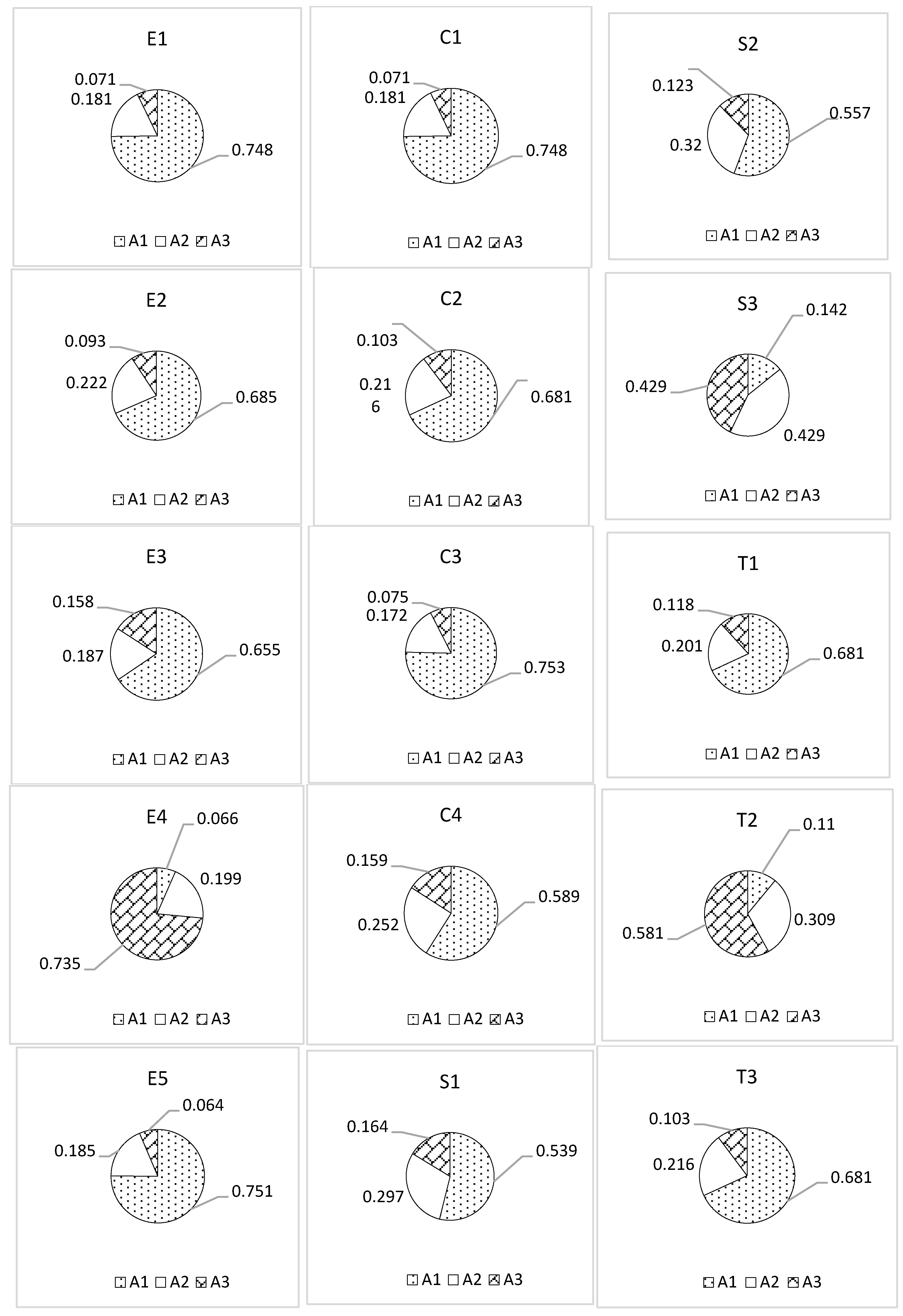
3.3. Decision of MSW Management Scenarios for Each Sub-Criterion Based on Source Separation Methods

The final evaluation of the results obtained as a result of the analyses carried out in accordance with the AHP was carried out in this section. In this chapter, it has been decided which disposal alternative is prioritized according to the source separation method. The final decision matrices for the evaluation of the MSW management scenarios for the sub-criteria are given in

Table A49. Priority matrix for evaluating the MSW management scenarios of environmental criteria for mixed collection.

Alternatives	E1 (0.390)	E2 (0.162)	E3 (0.318)	E4 (0.078)	E5 (0.052)	Overall Priority Vector
A1	0.748	0.685	0.655	0.065	0.751	0.655
A2	0.180	0.221	0.187	0.199	0.185	0.191
A3	0.072	0.094	0.158	0.736	0.064	0.154
						Σ = 1.000

,

Table A50. Priority matrix for evaluating the MSW management scenarios of economic criteria for mixed collection.

Alternatives	C1 (0.525)	C2 (0.273)	C3 (0.124)	C4 (0.078)	Overall Priority Vector
A1	0.748	0.681	0.753	0.589	0.699
A2	0.181	0.216	0.172	0.251	0.200
A3	0.071	0.103	0.075	0.160	0.101
					Σ = 1.000

,

Table A51. Priority matrix for evaluating the MSW management scenarios of social criteria for mixed collection.

Alternatives	S1 (0.587)	S2 (0.324)	S3 (0.089)	Overall Priority Vector
A1	0.539	0.557	0.142	0.510
A2	0.297	0.320	0.429	0.316
A3	0.164	0.123	0.429	0.174
				Σ = 1.000

and

Table A52. Priority matrix for evaluating the MSW management scenarios of technical criteria for mixed collection.

Alternatives	T1 (0.623)	T2 (0.239)	T3 (0.137)	Overall Priority Vector
A1	0.681	0.110	0.681	0.544
A2	0.201	0.309	0.216	0.229
A3	0.118	0.581	0.103	0.227
				Σ = 1.000

,

Table A53. Priority matrix for evaluating the MSW management scenarios of environmental criteria for binary collection.

Alternatives	E1 (0.046)	E2 (0.098)	E3 (0.160)	E4 (0.258)	E5 (0.438)	Overall Priority Vector
A1	0.748	0.685	0.655	0.065	0.751	0.553
A2	0.180	0.221	0.187	0.199	0.185	0.192
A3	0.072	0.094	0.158	0.736	0.064	0.255
						Σ = 1.000

,

Table A54. Priority matrix for evaluating the MSW management scenarios of economic criteria for binary collection.

Alternatives	C1 (0.116)	C2 (0.224)	C3 (0.601)	C4 (0.059)	Overall Priority Vector
A1	0.748	0.681	0.753	0.589	0.673
A2	0.181	0.216	0.172	0.252	0.217
A3	0.071	0.103	0.075	0.159	0.110
					Σ = 1.000

,

Table A55. Priority matrix for evaluating the MSW management scenarios of social criteria for binary collection.

Alternatives	S1 (0.466)	S2 (0.433)	S3 (0.101)	Overall Priority Vector
A1	0.539	0.557	0.142	0.507
A2	0.297	0.320	0.429	0.320
A3	0.164	0.123	0.429	0.173
				Σ = 1.000

and

Table A56. Priority matrix for evaluating the MSW management scenarios of technical criteria for binary collection.

Alternatives	T1 (0.213)	T2 (0.085)	T3 (0.702)	Overall Priority Vector
A1	0.681	0.110	0.681	0.632
A2	0.201	0.309	0.216	0.221
A3	0.118	0.581	0.103	0.147
				Σ = 1.000

, and

Table A57. Priority matrix for evaluating the MSW management scenarios of environmental criteria for S@3S collection.

Alternatives	E1 (0.035)	E2 (0.082)	E3 (0.147)	E4 (0.252)	E5 (0.484)	Overall Priority Vector
A1	0.748	0.685	0.655	0.065	0.751	0.558
A2	0.181	0.221	0.187	0.200	0.185	0.192
A3	0.071	0.094	0.158	0.735	0.064	0.250
						Σ = 1.000

,

Table A58. Priority matrix for evaluating the MSW management scenarios of economic criteria for triple collection.

Alternatives	C1 (0.097)	C2 (0.238)	C3 (0.617)	C4 (0.048)	Overall Priority Vector
A1	0.748	0.681	0.753	0.589	0.669
A2	0.180	0.216	0.172	0.252	0.219
A3	0.072	0.103	0.075	0.159	0.112
					Σ = 1.00

,

Table A59. Priority matrix for evaluating the MSW management scenarios of social criteria for triple collection.

Alternatives	S1 (0.472)	S2 (0.444)	S3 (0.084)	Overall Priority Vector
A1	0.539	0.557	0.142	0.514
A2	0.297	0.320	0.429	0.318
A3	0.164	0.123	0.429	0.168
				Σ = 1.000

and

Table A60. Priority matrix for evaluating the MSW management scenarios of technical criteria for triple collection.

Alternatives	T1 (0.230)	T2 (0.122)	T3 (0.648)	Overall Priority Vector
A1	0.681	0.110	0.681	0.611
A2	0.201	0.309	0.216	0.224
A3	0.118	0.581	0.103	0.165
				Σ = 1.000

, in terms of mixed collection, binary collection, and triple collection, respectively. Moreover, the graphs prepared for the MSW management scenario preferences created separately for each of the three main and four sub-criteria are given in Figure 4 (the graphs were prepared using the tables in Appendix C).

Figure 4 shows the final preference ranking of decision points according to the main and sub-criteria. The preference ranking of the MSW management scenarios changes according to the main criteria and first sub-criteria. In the mixed collection case from the main criteria, MSW management scenario A1 has the highest preference level according to the environmental criteria (0.655). In this case, the preference ranking of the MSW scenarios is A1 > A2 > A3. In the mixed collection case, MSW management scenario A1 has the highest preference level according to the economic criteria (0.699). In this case, the preference ranking of the MSW scenarios is A1 > A2 > A3. In the mixed collection case, MSW management scenario A1 has the highest preference level according to the social criteria (0.510). In this case, the preference ranking of the MSW scenarios is again A1 > A2 > A3. In the mixed collection case, MSW management scenario A1 has the highest preference level according to the technical criteria (0.544). In this case, the preference ranking of the MSW scenarios is A1 > A2 > A3. In the case of binary collection of the main criteria, MSW management scenario A1 has the highest preference level according to the environmental criteria (0.553). In this case, the preference order of the MSW scenarios is A1 > A3 > A2. In the case of binary collection, MSW management scenario A1 has the highest preference level again according to the economic criteria (0.673). In this case, the preference order of the MSW management scenarios is A1 > A2 > A3. In the case of binary collection, MSW management scenario A1 has the highest preference level again according to the social criteria (0.507). In this case, the preference order of the MSW scenarios is again A1 > A2 > A3. In the case of binary collection, MSW management scenario A1 has the highest preference level again according to the technical criteria (0.632). In this case, the preference order of the MSW scenarios is A1 > A2 > A3. In the triple collection case of the main criteria, MSW management scenario A1 has the highest preference level according to the environmental criteria (0.558). In this case, the preference order of the MSW scenarios is A1 > A2 > A3. In the triple collection case, MSW management scenario A1 has the highest preference level according to the economic criteria (0.669). In this case, the preference order of the MSW scenarios is A1 > A2 > A3. In the triple collection case, MSW management scenario A1 has the highest preference level according to the social criteria (0.514). In this case, the preference order of the MSW scenarios is again A1 > A2 > A3. In the triple collection case, MSW management scenario A1 has the highest preference level according to the technical criteria (0.611). In this case, the preference order of the MSW scenarios is A1 > A2 > A3.

3.4. Sensitivity Analysis

In MCDM analyses, sensitivity analyses are required to check the consistency of prioritization. This process is usually carried out by changing the criterion weights. Sensitivity analysis is used for this purpose [25]. Sensitivity analysis can be carried out by changing the weights of each criterion in the pairwise comparison process [26]. In this study, depending on the main criteria, which are the source separation methods, for each sub-criterion (E, C, S, and T) and the sub-criteria depending on these sub-criteria (E1–E5, C1–C4, S1–S3, and T1–T3). Separate sensitivity analyses were carried out in this study. First stage: the weight of each sub-criterion (e.g., E1) was reduced by 25%, the other criteria (E2, E3, E4, and E5) were kept constant, and the ranking of the MSW management scenarios was determined by performing sensitivity analysis. In the second stage, the weight of each sub-criterion (for example, C4) was increased by 25%, the other criteria (C1, C2, and C3) were kept constant, and the ranking of the alternatives was determined via sensitivity analysis. The results obtained for mixed, binary, and triple collection are given in Tables S1–S3 in the Supplementary Materials. When looking at the MSW management scenarios’ rankings, the rankings obtained as a result of the model and sensitivity analysis have not changed. The sensitivity analysis results first showed that for the main criterion of mixed collection at the source, the ranking of the MSW management scenarios did not change when the weights of each criterion changed (A1 > A2 > A3). In all 30 scenarios, A1 (MRF + SLF) ranked first, with the highest evaluation rate among the MSW management scenarios. Secondly, for the case of binary collection at the source (S@2S), the alternative sequence A1 > A3 > A2 was obtained in 10 out of 30 scenarios. The replacement of alternatives A2 and A3 took place in scenarios where the weights of environmental factors were changed. Thirdly, in the case of triple collection at the source (S@3S), the MSW management scenario order A1 > A3 > A2 was obtained in 10 out of 30 scenarios. The replacement of the MSW management scenarios A2 and A3 again occurred in scenarios where the weights of environmental factors were changed. For all three collection types, MSW management scenario A1 ranked first. The first sustainable solid waste management option in all 90 scenarios was determined as the A1 MSW management scenario, as in the model study. The results obtained from the analyses confirm the reliability of the results obtained via the AHP. In the study conducted by Alqaraleh et al. within the scope of MCDA, the MRF + CP + SLF option from the waste management scenarios was shown to be the most suitable option, as in this study. This shows that an approach within the scope of waste hierarchy is at the forefront in waste management processes [27].

4. Discussion

Nowadays, there is increasing interest in smart city technologies, which are understood to be useful in managing the MSW process in the most efficient way with a ZW vision. To successfully implement smart city technologies in the sustainable MSW process, stakeholders’ opinions must be taken into account, in addition to environmental, economic, technical, and social criteria. It is well known that the MCDM methods assist decision makers in choosing acceptable, affordable, and effective sustainable waste management alternatives. It is admirable that there are many efforts today to manage MSW using smart technologies [28,29,30,31,32,33]. However, the ability to use these technologies for their intended purpose depends on establishing waste management within a sustainable framework. Optimizing all processes from MSW formation to final disposal will contribute to achieving the purpose of the studies [1]. The expected successful management of MSW management options is closely related to how the waste is separated and collected at the point where it is generated. Even if all waste management processes are carried out in accordance with the technical criteria, both environmentally and economically, for example, route optimization [34], waste that requires one final step still needs to be disposed of through SLF [2]. The mixed collection of solid waste may not be relatively important in terms of SLF, but local regulations have imposed restrictions on the disposal of waste through SLF and are necessary for the sustainability of the environment. If separating recyclable waste is desired, then it is expected that binary separation will be carried out at the source and the two component groups will be collected separately for MRF, because with this method, it is possible to minimize possible value losses in the process of integration into secondary production processes that are intended to be recycled [35]. The TP can also be preferred for the energy recovery of waste without using additional energy [36]. If waste disposal through biological processes is desired (CP or BMP), then triple separation and separate collection are considered as source separation options that should be prioritized [37]. Holistic planning of sustainable waste management provides benefits not only economically, but also environmentally. In a study conducted within the scope of smart city solid waste management systems, the integrated use of smart technologies such as the internet of things, low-power wide area networks, and smart traffic systems was evaluated. The results obtained show that more efficient collection can be achieved and that collection costs can be reduced compared to the current curb collection [38].

In the literature, many studies considering separation options at the source based on MSW management alternatives can be found. In a study conducted using MCDM techniques, waste management options were investigated. In this study, no criteria were analyzed regarding source separation. According to the results obtained, waste management option priorities were determined as biomethanization, gasification (one of the thermal processes), and regular storage [39]. The aim of this study is to make a remarkable contribution to this gap in the literature. This study tries to put forward a perspective and a useful model that will help the studies carried out within the scope of zero waste management, sustainable waste management, and smart cities. No matter which of the three management alternatives highlighted here is used, it will be possible to obtain quantitative and solution-oriented results in all management options, including smart city studies. In this study, it has been determined that options other than mixed collection, which can be applied in all settlements, will make significant contributions to sustainable waste management processes. Numerous analyses considering expert opinions reveal that sustainable disposal alternatives may be possible with binary and triple separation at the source, and separate collection of separated wastes. This study is considered important in that it offers decision makers a solution that can be integrated into smart city technologies in the MSW management process.

5. Conclusions

In today’s world, the number of studies on smart waste management systems is increasing day by day due to the rapid development of information technology. The sustainability of smart waste management systems and their ability to meet expectations depends on whether waste management plans are made in accordance with technological and field requirements. Although theoretically sustainable waste management processes are well known, planning the points where waste is produced is of vital importance. In other words, deciding how to collect waste at the source is important for the success of zero waste, waste hierarchy, sustainable waste management, and smart waste management processes. This study reveals the effects of the way solid waste is collected at its source, which is thought to contribute to all sustainable waste management efforts, including smart waste management processes, on waste management alternatives. Detailed analysis of the selected method and three management scenarios for the separation of MSW at the source was made using the AHP, and an attempt was made to eliminate the deficiency in this regard. This study also reveals that when planning waste management processes, decision makers should first decide on the method or methods by which the waste will be collected at the source where it is generated, and plan management alternatives. In planning sustainable waste management systems to be proposed in future studies, it is thought that it would be appropriate to evaluate in detail the social, cultural, and waste potential components at the points where waste is generated, to do so in parallel with the feedback received, and to revise the plans in the light of the feedback.

References

1. Zaman, A.; Ahsan, T. Zero-Waste: Reconsidering Waste Management for the Future; Routledge: New York, NY, USA, 2020. [Google Scholar]
2. Tchobanoglous, G.; Theisen, H.; Vigil, S.A. Integrated Solid Waste Management: Engineering Principles and Management Issues; McGraw Hill Inc.: New York, NY, USA, 1993. [Google Scholar]
3. Apaydin, Ö.; Han, G.S.A. Analysis of Municipal Solid Waste Collection Methods Focusing on Zero-Waste Management Using an Analytical Hierarchy Process. Sustainability 2023, 15, 13184. [Google Scholar] [CrossRef]
4. Anagnostopoulos, T.; Zaslavsky, A.; Kolomvatsos, K.; Medvedev, A.; Amirian, P.; Morley, J.; Hadjieftymiades, S. Challenges and Opportunities of Waste Management in IoT-Enabled Smart Cities: A Survey. IEEE Trans. Sustain. Comput. 2017, 2, 275–289. [Google Scholar] [CrossRef]
5. Esmaeilian, B.; Wang, B.; Lewis, K.; Duarte, F.; Ratti, C.; Behdad, S. The future of waste management in smart and sustainable cities: A review and concept paper. Waste Manag. 2018, 81, 177–195. [Google Scholar] [CrossRef] [PubMed]
6. Saaty, R.W. The analytic hierarchy process—What it is and how it is used. Math. Modell. 1987, 9, 161–176. [Google Scholar] [CrossRef]
7. Saaty, T.L. That is not the analytical hierarchical process: What the AHP is and what it is not. J. Multi Criteria Decis. Anal. 1998, 6, 320–329. [Google Scholar]
8. Saaty, T.L. Rank from comparisons and from ratings in the analytic hierarchy/network processes. Eur. J. Oper. Res. 2006, 168, 557–570. [Google Scholar] [CrossRef]
9. Demircan, B.G.; Yetilmezsoy, K. Ahybrid fuzzy AHP-TOPSIS approach for implementation of smart sustainable waste management strategies. Sustainability 2023, 15, 6256. [Google Scholar] [CrossRef]
10. Tamasila, M.; Prostean, G.; Ivascu, L.; Cioca, L.I.; Draghici, A.; Diaconescu, A. Evaluating and prioritizing municipal solid waste management-related factors in Romania using fuzzy AHP and TOPSIS. J. Intell. Fuzzy Syst. 2020, 38, 6111–6127. [Google Scholar] [CrossRef]
11. Shahnazari, A.; Pourdej, H.; Kharage, M.D. Ranking of organic fertilizer production from solid municipal waste systems using analytic hierarchy process (AHP) and VIKOR models. Biocatal. Agric. Biotechnol. 2021, 32, 101946. [Google Scholar] [CrossRef]
12. Xi, H.; Li, Z.; Han, J.; Shen, D.; Li, N.; Long, Y.; Chen, Z.; Xu, L.; Zhang, X.; Niu, D.; et al. Evaluating the capability of municipal solid waste separation in China based on AHP-EWM, BP neural network. Waste Manag. 2022, 139, 208–216. [Google Scholar] [CrossRef]
13. AlHumid, H.A.; Haider, H.; AlSaleem, S.S.; Shafiquzamman, M.; Sadiq, R. Performance indicators for municipal solid waste management systems in Saudi Arabia: Selection and ranking using fuzzy AHP and PROMETHEE II. Arab. J Geosci. 2019, 12, 491. [Google Scholar] [CrossRef]
14. Zhou, X.; Xiang, X.; Wang, C.; Deng, Z.; Peng, D.; Li, Y.; Zhou, J. Study on evaluation method for the rural solid waste fixed bed gasification using the AHP-FCE based on exergy analysis. Int. J. Exergy 2023, 40, 365–391. [Google Scholar] [CrossRef]
15. Ampofo, S.; Issifu, J.S.; Kusibu, M.M.; Mohammed, A.S.; Adiali, F. Selection of the final solid waste disposal site in the Bolgatanga municipality of Ghana using analytical hierarchy process (AHP) and multi-criteria evaluation (MCE). Heliyon 2023, 9, e18558. [Google Scholar] [CrossRef]
16. Karimzadeh, K.; Tehrani, G.M.; Khaloo, S.S.; Vaziri, M.H.; Ardeh, S.A.; Saeedi, R. Quantitative assessment of health, safety, and environment (HSE) resilience based on the Delphi method and analytic hierarchy process (AHP) in municipal solid waste management system: A case study in Tehran. Environ. Health Eng. Manag. J. 2023, 10, 237–247. [Google Scholar] [CrossRef]
17. Torkayesh, A.E.; Rajaeifar, M.A.; Rostom, M.; Malmir, B.; Yazdani, M.; Suh, S.; Heidrich, O. Integrating life cycle assessment and multi criteria decision making for sustainable waste management: Key issues and recommendations for future studies. Renew. Sustain. Energy Rev. 2022, 168, 112819. [Google Scholar] [CrossRef]
18. Kumar, A.; Dixit, G. A novel hybrid MCDM framework for WEEE recycling partner evaluation on the basis of green competencies. J. Clean. Prod. 2019, 241, 118017. [Google Scholar] [CrossRef]
19. Çoban, A.; Firtina Ertiş, I.; Ayvaz Cavdaroglu, N. Municipal solid waste management via multi-criteria decision making methods: A case study in Istanbul, Turkey. J. Clean. Prod. 2018, 180, 159–167. [Google Scholar] [CrossRef]
20. Khan, I.; Kabir, Z. Waste-to-energy generation technologies and the developing economies: A multi-criteria analysis for sustainability assessment. Renew. Energy 2020, 150, 320–333. [Google Scholar] [CrossRef]
21. Topaloglu, M.; Yarkin, F.; Kaya, T. Solid waste collection system selection for smart cities based on a type-2 fuzzy multi-criteria decision technique. Soft Comput. 2018, 22, 4879–4890. [Google Scholar] [CrossRef]
22. Singh, A. Solid waste management through the applications of mathematical models. Resour. Conserv. Recycl. 2019, 151, 104503. [Google Scholar] [CrossRef]
23. Al-Harbi, K.M.A.S. Application of the AHP in project management. Int. J. Proj. Manag. 2001, 19, 19–27. [Google Scholar] [CrossRef]
24. Thomas, L.; Saaty, T.L.; Vargas, L.G. Models, Methods, Concepts and Applications of the Analytic Hierarchy Process, 2nd ed.; Springer: New York, NY, USA, 2012. [Google Scholar]
25. 1000minds. Decision-Making/Multi-Criteria Decision Analysis (MCDA/MCDM). Available online: https://www.1000minds.com/decision-making/what-is-mcdm-mcda (accessed on 21 March 2025).
26. Goyal, S.; Garg, D.; Luthra, S. Sustainable production and consumption: Analysing barriers and solutions for maintaining green tomorrow by using fuzzy-AHP–fuzzy-TOPSIS hybrid framework. Environ. Dev. Sustain. 2021, 23, 16934–16980. [Google Scholar] [CrossRef]
27. Alqaraleh, L.; Abu Hajar, H.A.; Matarneh, S. Multi-criteria sustainability assessment of solid waste management in Jordan. J. Environ. Manag. 2024, 366, 121929. [Google Scholar] [CrossRef]
28. Syed, A.S.; Sierra-Sosa, D.; Kumar, A.; Elmaghraby, A. 2021 IoT in smart cities: A survey of technologies, practices and challenges. Smart Cities 2021, 4, 429–475. [Google Scholar] [CrossRef]
29. Gopikumar, S.; Raja, S.; Robinson, Y.H.; Shanmuganathan, V.; Rho, S. A method of landfill leachate management using internet of things for sustainable smart city development. Sustain. Cities Soc. 2020, 66, 102521. [Google Scholar] [CrossRef]
30. Sheng, T.J.; Islam, M.S.; Misran, N.; Baharuddin, M.H.; Arshad, H.; Islam, R.; Chowdhury, M.E.H.; Rmili, H. An internet of things based smart waste management system using lora and tensorflow deep learning model. IEEE Access 2020, 8, 148793–148811. [Google Scholar] [CrossRef]
31. Gupta, Y.S.; Mukherjee, S.; Dutta, R.; Bhattacharya, S. A blockchain-based approach using smart contracts to develop a smart waste management system. Int. J. Environ. Sci. Technol. 2022, 19, 7833–7856. [Google Scholar] [CrossRef]
32. Chauhan, A.; Jakhar, S.K.; Chauhan, C. The interplay of circular economy with industry 4.0 enabled smart city drivers of healthcare waste disposal. J. Clean. Prod. 2021, 279, 123854. [Google Scholar] [CrossRef]
33. Seker, S. IoT based sustainable smart waste management system evaluation using MCDM model under interval-valued q-rung orthopair fuzzy environment. Technol. Soc. 2022, 71, 102100. [Google Scholar] [CrossRef]
34. Apaydin, Ö.; Gönüllü, M.T. Emission control with route optimization in solid waste collection process: A case study. Sadhana-Acad. Proc. Eng. Sci. 2008, 33, 71–82. [Google Scholar] [CrossRef]
35. Rhvner, C.R.; Schwartz, L.J.; Wenger, R.B.; Kohrell, M.G. Waste Management and Resource Recovery, 1st ed.; CRC Press: Boca Raton, FL, USA, 1995. [Google Scholar]
36. Tanner, R. Die Entwicklung der Von Roll Müllverbrennungsanlagen. Schweiz. Bauztg. 1965, 16, 251–260. [Google Scholar]
37. Öztürk, İ. Katı Atık Yönetimi ve AB Uygulamaları; Teknik Kitaplar Serisi 2; İSTAÇ AŞ: Istanbul, Türkiye, 2010. [Google Scholar]
38. Henaien, A.; Ben Elhadj, H.; Fourati, L.C. A sustainable smart IoT-based solid waste management system. Future Gener. Comput. Syst. Int. J. Sci. 2024, 157, 587–602. [Google Scholar] [CrossRef]
39. Mujtaba, M.A.; Munir, A.; Imran, S.; Nasir, M.K.; Muhayyuddin, M.G.; Javed, A.; Mehmood, A.; Habila, M.A.; Fayaz, H.; Qazi, A. Evaluating sustainable municipal solid waste management scenarios: A multicriteria decision making approach. Heliyon 2024, 10, e25788. [Google Scholar] [CrossRef] [PubMed]
Figure 1. Hierarchy of this model.
Sustainability 17 03868 g001
Figure 2. Conceptual diagram of the AHP used in decision making in this study.
Sustainability 17 03868 g002
Figure 3. Pairwise comparison of sub-criteria based on MSW management scenarios.
Sustainability 17 03868 g003
Figure 4. Decision of MSW management scenarios for each sub-criterion based on source separation methods.
Sustainability 17 03868 g004aSustainability 17 03868 g004b