Societal Impacts of Renewable Energy Consumption and Transport CO₂ Emissions in New Zealand

Abstract

Life expectancy and mortality rates are important indicators of public health and societal well-being, which are heavily influenced by environmental and economic factors. This study estimates the impacts of renewable energy consumption, transportation CO₂ emissions, and other variables on life expectancy and mortality in New Zealand using the dynamic autoregressive distributed lag simulations methodology during 1972–2022. The findings indicate that a 1% increase in renewable energy consumption and household expenditure leads to rises in life expectancy of 0.03% and 0.005%, respectively, in the long run. Urbanisation can also boost life expectancy in the long run by 0.43% if its value rises by 1%. However, if CO₂ emissions from the transport sector rise by 1% in the long run, it will contribute to a 0.07% decrease in life expectancy. However, the short-run results show that trade household expenditure, public health expenditure, and renewable energy consumption increase life expectancy, while capital formation and transport CO₂ emissions reduce it, but with lower impacts. The mortality results show that trade, public health expenditures, urbanisation, and renewable energy consumption can reduce mortality in the long run by 0.59%, 0.52%, 16%, and 0.66%, respectively, when their values increase by 1%, while transport CO₂ emissions increase it by 1.6%. However, capital formation can decrease mortality in the long run. It declines mortality by 0.21% when increased by 1%. These findings suggest the crucial role of renewable energy consumption and public health expenditure in decreasing mortality rates and improving life expectancy in New Zealand. Policymakers must prioritize these variables to achieve meaningful improvements in public health outcomes.

1. Introduction

Increases in human activities and economic growth have led to a significant rise in transportation use, resulting in increased demand for fossil fuels and, consequently, higher greenhouse gas emissions, particularly CO₂ emissions, in the atmosphere. In addition to transport GDP, urbanisation is another major contributor to the increases in transport CO₂ emissions in the short and long runs [1]. UN reports indicate that air pollution causes approximately 7 million premature deaths each year, making it a major environmental threat to public health worldwide [2]. This report also indicates that in Asia and the Pacific, residential sources are the largest contributors to particle pollution, accounting for 12.47 micrograms per cubic meter of air (µg/m³), whereas the transport contribution is approximately 4.02 µg/m³ [2].

In New Zealand, transport was also responsible for a large share of emissions. The country produced about 28.7 million tonnes of CO₂ emissions, of which the transport sector contributed to around 14.6 million tonnes of CO₂ (51.02% of total CO₂ emissions), followed by manufacturing and construction (20.48%) (Figure 1). New Zealand has high transport emissions per person, at 2.7 tonnes of CO₂ equivalent, which is above the developed country average of 2 tonnes of CO₂ equivalent [3]. Reports also show that New Zealand has higher per capita gross emissions of all gases than the developed countries. In 2021, it was 15.1 tonnes of carbon dioxide equivalent per capita, higher than the developed world average of 8.8 tonnes of CO₂ equivalent [4]. Figure 2 presents the trend of major air pollutants in New Zealand from 2012 to 2019. It shows that carbon monoxide (CO) is the most common air pollutant in the country, followed by nitrogen oxides (NO_x) and particulate matter (PM₁₀).

To combat climate change, policies that affect both supply and demand, particularly in the transport sector, must be implemented [6] while considering the economic and social consequences [7]. Strict policies could negatively impact households without adequate support, but rising fossil fuel prices could reduce fossil fuel consumption and lower CO₂ emissions [8].

A strong relationship exists between health expenditures and life expectancy with CO₂ emissions [9,10,11]. Transportation-related air pollution, including particulate matter, nitrogen oxides, and volatile organic compounds, can significantly affect mortality and life expectancy in New Zealand. This occurs through various pathways, mainly by worsening respiratory and cardiovascular diseases [12].

Research shows that increased environmental degradation, particularly CO₂ emissions, can significantly diminish individuals’ average lifespans [13]. Moreover, investments in health expenditures and population growth contribute positively to enhancing life expectancy [14,15]. This emphasises the critical point that by allocating more resources to the healthcare sector, governments can effectively save more lives and extend human longevity [16]. This also lowers mortality rates, allowing for an increase in life expectancy [15].

The crude death rate in New Zealand has increased in recent years, from 31.6 thousand in 2015 to 32.6 thousand in 2020, and then jumped to 38.6 thousand and 37.9 thousand in 2020 and 2023, respectively [17]. However, this rate is lower than the average OECD rate.

Therefore, this study aims to identify the relationship between important economic and environmental variables and health-related indicators, namely life expectancy and mortality rates. Thus, it investigates how transport CO₂ emissions, renewable energy consumption (including all types of renewable energy sources), and other economic indicators, such as trade and health expenditure, influence life expectancy and mortality rates in New Zealand.

We use transport CO₂ emissions as a proxy for the use of renewable energy sources (such as biofuels) and electric vehicles in the transport sector, as they can significantly reduce CO₂ emissions [18]. This means that the reduced use of renewable energy sources and electric vehicles in this sector increases CO₂ emissions, leading to a negative effect on life expectancy and contributing to a higher mortality rate. It is important to note that while transportation CO₂ emissions may not directly affect life expectancy and mortality, their toxic air pollutants impact health-related issues, which, in turn, influence mortality and life expectancy [19,20].

Additionally, we utilize life expectancy and mortality rates as indicators of overall well-being and societal costs. Mitigating environmental challenges, including CO₂ emissions and climate change, enhances population health and societal well-being [21,22,23].

This study contributes to the current literature by examining the effects of transport CO₂ emissions, gross fixed capital formation, trade, and household expenditure—variables that have rarely been explored in this context. This is due to the fact that other important variables, such as GDP, total CO₂ emissions, population, and others, have been widely used in the literature. Consequently, to prevent presenting redundant results, we employed less frequently used variables in this study. Furthermore, it makes a significant contribution by analysing the influence of multiple factors on both mortality rates and life expectancy, areas that have also received limited attention in the current literature.

The organisation of this study is as follows. Section 2 provides a review of the existing literature. Section 3 discusses the methodology and data. Section 4 presents the results along with their discussions, and Section 5 discusses the conclusions and policy suggestions.

2. Literature Review

Numerous studies have been conducted over the years to investigate the complex relationships among environmental, economic, and social factors influencing indicators such as life expectancy and mortality. Notably, CO₂ emissions and their associated environmental issues have been extensively studied for their direct and indirect impacts on human health.

Research shows that CO₂ emissions are directly linked to respiratory and cardiovascular diseases, ultimately reducing life expectancy by compromising air quality and contributing to an increase in chronic illnesses [24]. More recent studies, such as those by Burnett et al. [25], provide accurate measurements of the global disease burden associated with air pollution, highlighting its significant impact on mortality rates. Furthermore, the rising levels of CO₂ emissions are resulting in more frequent heatwaves, which particularly endanger vulnerable populations, such as the elderly and those with pre-existing health conditions [26,27].

Other research has investigated how various factors affect life expectancy and mortality, both of which are important indicators of societal well-being. These studies highlight that, while urbanisation improves access to healthcare and social services, it has a complex impact on life expectancy [28]. Ahmad et al. [29] found a negative relationship between urbanisation and life expectancy, whereas Tripathi and Maiti [30] demonstrated that the impact of urbanisation on health outcomes is determined by urbanisation management, which, in well-managed countries, has a positive impact on people’s health.

Many studies suggest that the use of renewable energy and increased healthcare spending are associated with longer life expectancy [31,32,33]. The consumption of renewable energy is associated with improved environmental quality, which in turn lowers mortality rates by reducing pollution, particularly in countries that heavily rely on fossil fuels [34,35]. While trade and gross fixed capital formation contribute to economic growth, their direct effects on mortality and life expectancy are affected by factors such as income distribution, healthcare investments, and infrastructure enhancements [36,37].

Research also shows that trade has a complex impact on mortality, influencing both economic growth and environmental conditions. For example, Cícero et al. [38] showed that trade liberalization improves healthcare infrastructure, including medical technologies and pharmaceuticals, resulting in lower mortality rates. Other studies, however, suggest that the increase in industrial production caused by trade expansion may lead to environmental degradation and pollution, which can increase mortality rates, particularly in developing countries [39,40]. Furthermore, gross fixed capital formation, which represents infrastructure investments, has a significant impact on mortality reduction by improving healthcare access and raising living standards [41,42].

Health spending has a significant impact on the accessibility and quality of healthcare services, as well as mortality rates. Higher health expenditures are consistently associated with lower mortality rates and longer life expectancy, owing to improved medical care and robust health systems [43,44]. While inefficiencies and corruption can mitigate the effects of health spending, targeted investments in primary healthcare have been shown to reduce mortality rates and increase life expectancy, particularly in cases involving preventable diseases [45,46].

Many studies have investigated the impacts of GDP, total CO₂ emissions, global CO₂ concentration, and population on life expectancy, and have found varying effects. For example, Liu et al. [31] discovered that both GDP and population exhibit a negative relationship with life expectancy. According to the study by Polcyn et al. [32], GDP has a positive impact, while population has a negative effect on life expectancy. Vatamanu et al. [37] explored the influence of institutional quality on life expectancy and found that it can enhance life expectancy in EU countries. Additionally, Ibrahim and Ajide [35] examined the influence of income on life expectancy, revealing a positive impact. Nikita et al. [42] also reported the adverse effects of infrastructure, including healthcare, education, and sanitation, on mortality. Das and Debanth [44] demonstrated that increases in CO₂ emissions can enhance life expectancy in India up to a certain threshold, beyond which it has an inverse effect. An improvement in transportation infrastructure investment can lead to reduced mortality rates [47].

The literature reveals that many studies predominantly focus on the relationship between CO₂ emissions, population, and gross domestic product (GDP) and mortality or life expectancy. However, a significant limitation of these studies is their tendency to examine only one aspect of societal well-being—either mortality or life expectancy. Additionally, they often overlook a broader array of economic and non-economic factors. To address these gaps, the current study investigates a diverse range of variables, including trade, gross fixed capital formation, household expenditure, urbanisation, renewable energy consumption, and public health expenditures, with a particular emphasis on transport CO₂ emissions. Notably, the inclusion of household expenditures and transport CO₂ emissions represents a fresh approach that has been scarcely addressed in the existing literature.

3. Methodology

This study employs the autoregressive distributed lag (ARDL) approach to conduct dynamic simulations that evaluate the impact of renewable energy consumption and transport-related CO₂ emissions on two vital components of social well-being. By leveraging this technique, we effectively simulate how a particular shock or change in transport-related CO₂ emissions and renewable energy consumption influences life expectancy and mortality rates.

A multitude of studies have utilized diverse methodologies to investigate the influence of various factors on life expectancy. For example, Das and Debanth [44] and Osabohien et al. [45] analysed the effects of CO₂ emissions and health expenditures on life expectancy through the ARDL model. Meanwhile, Mahalik et al. [16] explored the relationships between consumption-based CO₂ emissions, urbanisation, and life expectancy across 68 countries.

Murthy et al. [15] conducted a comprehensive study on the impact of CO₂ emissions, GDP, health expenditure, and population dynamics on life expectancy in D-8 countries. In a related investigation, Emodi et al. [48] analysed how transport CO₂ emissions and transport infrastructure relate to life expectancy and mortality rates across 76 nations. Additionally, many studies examined the effects of renewable energy consumption, CO₂ emissions, and urbanisation on life expectancy and mortality rates [49,50,51,52].

Further research such as that of Rasoulinezhad et al. [53] has assessed the influences of economic growth, inflation rates, per capita CO₂ emissions, the human development index, population growth, and fossil fuel energy consumption. Khatri et al. [54] also analysed the relationship between economic growth and health expenditure with child mortality in Nepal. Building on this body of literature, we introduce the models for the current study, presented as Equations (1) and (2).

LEXP_t = f (TRAD_t, GFCF_t, HCON_t, HEXP_t, URB_t, REC_t, TRCO_2t)

(1)

MORT_t = f (TRAD_t, GFCF_t, HCON_t, HEXP_t, URB_t, REC_t, TRCO_2t)

(2)

where LEXP_t and MORT_t are the life expectancy at birth (in years) and mortality (per 1000 adults) in New Zealand in year t, respectively. TRAD_t is the total export and import of the country in year t (% of GDP), GFCF_t denotes gross fixed capital formation in year t (constant 2015 USD), HCON_t is the households’ expenditure (constant 2015 USD), HEXP_t is the government health expenditure (% of GDP), URB_t is the percentage of the population living in urban areas, REC_t indicates the total of all renewable energy sources in the country in year t (Petajoules), and TRCO_2t shows the total CO₂ emissions from the transport sector (tonnes) in year t.

The data for all variables in this study cover the years 1972–2022 and were gathered from the World Development Indicators of the World Bank. After transforming the variables into their (natural) logarithmic values, Equations (1) and (2) are linearised and written as follows:

$$\begin{array}{c}LnLEX{P}_t=a_0+a_{1}Ln{TRAD}_t+a_{2}LnGFC{F}_t+a_{3}LnHCO{N}_t+a_{4}LnHEX{P}_t\\ +a_{5}Ln{URB}_t+a_{6}Ln{REC}_t+a_{7}Ln{TRCO}_{2t}+e_t\end{array}$$

(3)

$$\begin{array}{c}Ln{MORT}_t=b_0+b_{1}LnT{RAD}_t+b_{2}LnGFC{F}_t+b_{3}LnHCO{N}_t+\\ b_{4}LnHEX{P}_t+b_{5}Ln{URB}_t+b_{6}Ln{REC}_t+bLn{TRCO}_{2t}+u_t\end{array}$$

(4)

In Equations (3) and (4), t represents the time subscript, while e_t and u_t denote the error terms. The parameters for estimation are represented by as and bs.

3.1. Estimation Strategy

Utilizing the autoregressive distributed lag (ARDL) model, we will investigate both the short-run and long-run relationships among the proposed variables in Equations (3) and (4). After verifying the essential statistical properties of the data series, we will implement the ARDL bounds testing methodology introduced by Pesaran et al. [49]. This technique excels in addressing variables that exhibit both stationary and non-stationary characteristics, accommodating those integrated up to order 1 or even those that are fractionally integrated (different orders of integration). It can estimate both short- and long-run dynamics and is robust in small samples [19]. The ARDL approach yields unbiased and efficient estimators, effectively addressing concerns about autocorrelation. Even with its benefits, testing for a long-run cointegration using the ARDL framework still demands considerable effort. The test statistic exhibits a nonstandard distribution that fluctuates depending on various model attributes and the data itself, including the order of integration of the variables [20].

The process consists of two crucial steps: In the first step, we will examine the predicted long-run relationships among our variables, as outlined by the theory. If a long-run relationship is confirmed, we will then proceed to the second step, where we will estimate the relevant parameters and the error correction framework.

To assess whether our variables possess unit roots, we performed the Augmented Dickey–Fuller (ADF) test and the Phillips–Perron test, utilizing the modified Akaike Information Criterion (AIC) to determine the appropriate lag length. If the variables are found to be stationary either at the level [I(0)] or at the first difference [I(1)], we can then proceed to employ the ARDL bounds testing approach to identify the presence of cointegration.

3.1.1. ARDL Framework for Estimation

Following the framework established by Pesaran et al. [55], the error correction representation of the ARDL model for Equations (3) and (4) can be presented as follows:

$$\begin{array}{c}∆LnLEX{P}_t={\alpha }_0+{\sum }_{i=1}^p{\alpha }_1∆Ln{LEXP}_{t-i}+{\sum }_{i=0}^p{\alpha }_2∆Ln{TRAD}_{t-i}+\\ {\sum }_{i=0}^p{\alpha }_3∆LnGFC{F}_{t-i}+{\sum }_{i=0}^p{\alpha }_4∆LnHCO{N}_{t-i}+{\sum }_{i=0}^p{\alpha }_5∆LnHEX{P}_{t-i}+\\ {\sum }_{i=0}^p{\alpha }_6∆Ln{URB}_{t-i}+{\sum }_{i=0}^p{\alpha }_7∆Ln{REC}_{t-i}+{\sum }_{i=0}^p{\alpha }_8∆Ln{TRCO}_{2t-i}+\\ {\beta }_{1}LnT{RAD}_t+{\beta }_{2}LnGFC{F}_t+{\beta }_{3}LnHCO{N}_t+{\beta }_{4}LnHEX{P}_t+{\beta }_{5}Ln{URB}_t+\\ {\beta }_{6}Ln{REC}_t+{\beta }_{7}Ln{TRCO}_{2t}+{\epsilon }_t\end{array}$$

(5)

$$\begin{array}{c}∆Ln{MORT}_t={\gamma }_0+{\sum }_{i=1}^p{\gamma }_1∆Ln{MORT}_{t-i}+{\sum }_{i=1}^p{\gamma }_2∆Ln{TRAD}_{t-i}+\\ {\sum }_{i=1}^p{\gamma }_3∆LnGFC{F}_{t-i}+{\sum }_{i=1}^p{\gamma }_4∆LnHCO{N}_{t-i}+{\sum }_{i=0}^p{\gamma }_5∆LnHEX{P}_{t-i}+\\ {\sum }_{i=0}^p{\gamma }_6∆Ln{URB}_{t-1}+{\sum }_{i=0}^p{\gamma }_7∆Ln{REC}_{t-1}+{\sum }_{i=0}^p{\gamma }_8∆Ln{TRCO}_{2t-i}+\\ {\delta }_{1}Ln{TRAD}_t+{\delta }_{2}LnGFC{F}_t+{\delta }_{3}LnHCO{N}_t+{\delta }_{4}LnHEX{P}_t+{\delta }_{5}Ln{URB}_t+\\ {\delta }_{6}LnRECO{N}_t+{\delta }_{7}Ln{TRCO}_{2t}+{ϵ}_t\end{array}$$

(6)

In the above equations, α₀ and ${\gamma }_0$ represent the intercept terms, while α_i and ${\gamma }_i$ (for i = 1, …, 8) denote the short-run coefficients for each variable. The parameter β_i and ${\delta }_i$ (for i = 1, …, 7) correspond to the long-run coefficient, and ε_t and ${ϵ}_{\mathrm{t}}$ signify the error terms.

3.1.2. Novel Dynamic ARDL Simulations: An Extension

Recent research has highlighted the complexity of the ARDL model [56,57], showcasing innovative dynamic simulations that effectively capture how changes in regressors affect the independent variable. These simulations serve as valuable tools to address and resolve the inherent challenges of the model [58].

The simulations will incorporate impulse response diagrams, enabling us to visually verify how the time profile of the independent variable has evolved due to alterations in the regressors. Given the scarcity of literature on this approach, and the even fewer studies on specific applications, our research makes a vital contribution to advancing knowledge in this particular methodology. The innovative dynamic ARDL simulations will be grounded in the model developed by Jordan and Philips [57], utilizing Equations (3) and (5) to derive Equation (7), and Equations (4) and (6) to produce Equation (8):

$$\begin{array}{c}∆LnLEX{P}_t={\alpha }_0+{\alpha }_1∆Ln{TRAD}_t+{\alpha }_2∆LnGFC{F}_t+{\alpha }_3∆LnHCO{N}_t+\\ {\alpha }_4∆LnHEX{P}_t+{\alpha }_5∆Ln{URB}_t+{\alpha }_6∆Ln{REC}_t+{\alpha }_7∆Ln{TRCO}_{2t}+\\ {\beta }_{1}Ln{TRAD}_{t-1}+{\beta }_{2}LnGFC{F}_{t-1}+{\beta }_{3}LnHCO{N}_{t-1}+{\beta }_{4}LnHEX{P}_{t-i}+\\ {\beta }_{5}Ln{URB}_{t-1}+{\beta }_{6}Ln{REC}_{t-1}+{\beta }_{7}Ln{TRCO}_{2t-1}+{\epsilon }_t\end{array}$$

(7)

$$\begin{array}{c}∆Ln{MORT}_t={\gamma }_0+{\gamma }_1∆Ln{TRAD}_t+{\gamma }_2∆LnGFC{F}_t+{\gamma }_3∆LnHCO{N}_t+\\ {\gamma }_4∆LnHEX{P}_t+{\gamma }_5∆LnURBA{N}_t+{\gamma }_6∆Ln{REC}_t+{\gamma }_7∆Ln{TRCO}_{2t}+\\ {\delta }_{1}Ln{TRAD}_{t-1}+{\delta }_{2}LnGFC{F}_{t-1}+{\delta }_{3}LnHCO{N}_{t-1}+{\delta }_{4}LnHEX{P}_{t-1}+\\ {\delta }_{5}Ln{URB}_{t-1}+{\delta }_{6}Ln{REC}_{t-1}+{\delta }_{7}Ln{TRCO}_{2t-1}+{ϵ}_t\end{array}$$

(8)

It is important to highlight that α₀ and ${\gamma }_0$ serve as the intercepts. As previously explored in Equations (5) and (6), α_i’s and ${\gamma }_{\mathrm{i}}$’s represent the short-run coefficients, while β_is and ${\delta }_{\mathrm{i}}$’s correspond to the long-run coefficients within the dynamic ARDL simulation model.

4. Results and Discussion

4.1. Basic Data Characteristics and Pre-Estimation Tests

Before estimating the ARDL models, it is necessary to discuss and perform some pre-estimation tests to determine whether the values of variables are consistent with the theory of the model or not. To do this, we first estimate the descriptive statistics of the variables, which describe the major characteristics of the data.

Table 1. Descriptive statistics of variables in both models.

	HCON	GFCF	TRAD	TRCO2	LEXP	MORT	REC	URB	HEXP
Mean	15.73	24.12	3.74	16.38	4.38	5.09	3.51	4.46	1.86
Median	15.41	24.15	3.74	16.43	4.38	5.07	3.58	4.46	1.85
Maximum	18.06	24.72	3.95	16.60	4.42	5.41	3.74	4.47	2.05
Minimum	14.34	23.34	3.57	16.06	4.33	4.87	3.09	4.45	1.71
Std. Dev.	0.93	0.38	0.09	0.14	0.03	0.18	0.18	0.00	0.12
Skewness	1.08	−0.21	0.27	−0.56	−0.28	0.39	−0.83	−0.35	0.20
Kurtosis	3.51	2.05	3.03	2.71	1.70	1.72	2.43	2.97	1.42

presents the estimated values for key descriptive statistics, including means, maximum and minimum values, and standard deviations for the selected variables. Next, we need to check the stationarity of the variables using unit root tests to avoid spurious regression. Once all model variables passed the stationarity tests, we checked for long-run cointegration among all variables in the model using the bound test to estimate the ARDL model. Finally, after estimating the model, we need to perform several diagnostic tests to ensure that the overall results of the model are correct.

According to the methodology outlined, the bounds test framework is suitable for variables that are either integrated at level I(0) or first difference I(1). To determine the order of integration among the variables and prevent incorrect results, unit root tests were conducted. The null hypothesis of the presence of a unit root test was evaluated against the alternative hypothesis of stationarity using the Augmented Dickey–Fuller (ADF) and Phillips–Perron tests, with the findings presented in

Table 2. Unit root test results.

	ADF				Phillips–Perron
	Intercept		Intercept and Trend		Intercept		Intercept and Trend
	I(0)	I(1)	I(0)	I(1)	I(0)	I(1)	I(0)	I(1)
HCON	−1.830	−9.173 *	−2.569	−9.259 *	−1.668	−9.924 *	−2.412	−11.867 *
GFCF	−0.327	−7.504 *	−2.704	−7.595 *	−0.327	−7.551 **	−2.745	−7.595 *
TRAD	−3.404 **	−7.928 *	−3.941 **	−7.874 *	−3.404 **	−11.037 *	−3.995 **	−13.743 *
TRCO2	−2.177	−5.561 *	−0.231	−5.738 *	−2.177	−5.548 *	−0.479	−5.723 *
LEXP	−0.521	−9.874 *	−2.279	−9.875 *	−0.524	−9.991 *	−2.308	−10.130 *
MORT	−1.111	−8.959 *	−0.551	−8.986 *	0.840	−9.074 *	−1.180	−9.153 *
RENC	−4.531 *	−5.680 *	−4.415 *	−5.476 *	−3.746 *	−5.956 *	−4.051 **	−5.576 *
URB	0.759	−2.854 ***	−1.713	−2.434	−2.865 ***	−2.914 ***	−1.808	−2.634
HEXP	−0.026	−5.556 *	−1.664	−5.590	−0.296	−5.547 *	−1.884	−5.593 *
	−0.992	−7.325 *	−3.079 *	−7.330 *	−1.178	−7.801 *	3.115	−7.751 *

Note: * p < 0.01, ** p < 0.05, *** p < 0.1.

.

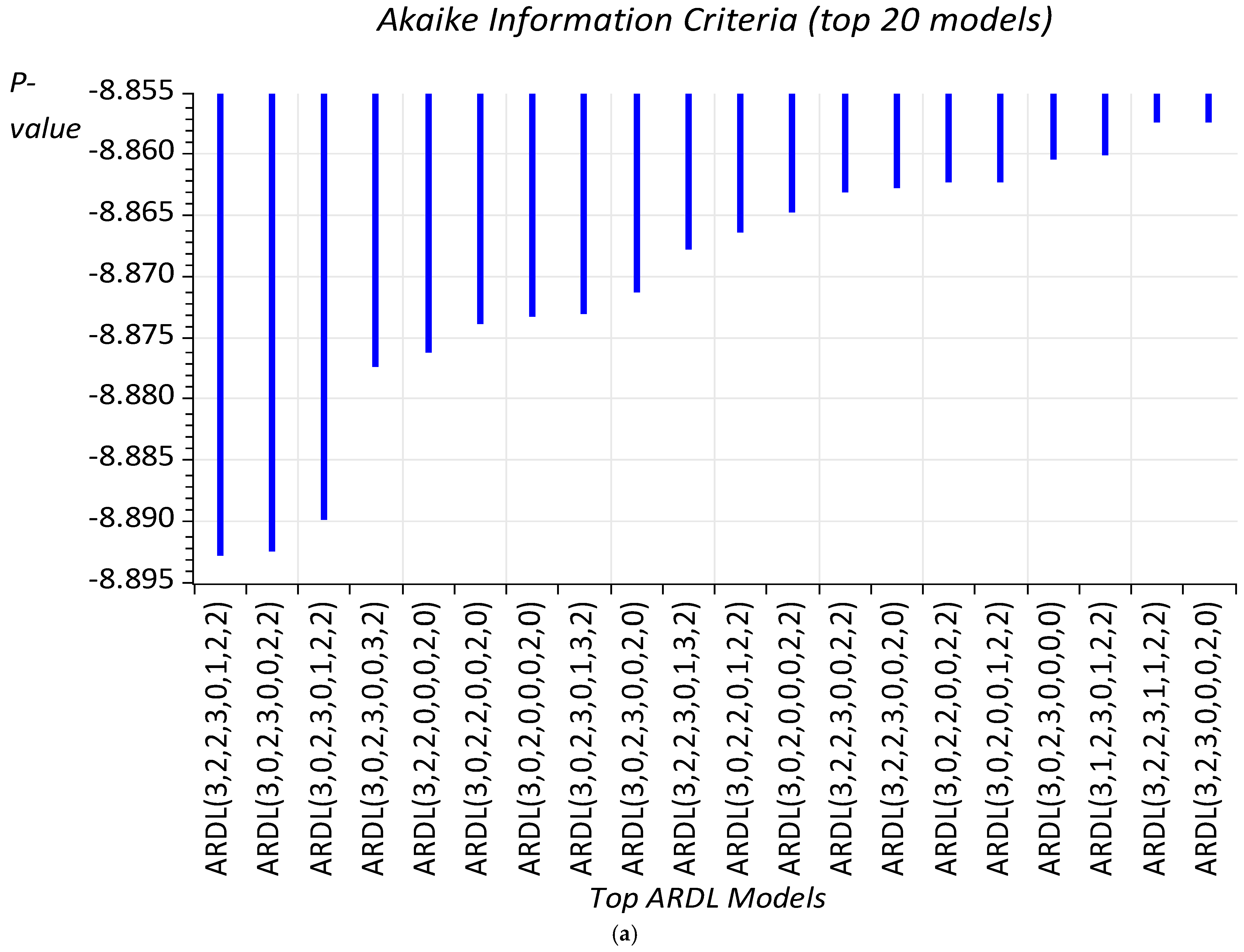
Through unit root testing on the selected variables in our study, we discovered that all variables exhibit stationarity after the first difference, except trade and renewable energy consumption, which are stationary at both I(0) and I(1). Consequently, we can confidently move forward with the ARDL estimation framework, particularly since our dependent variables—life expectancy and mortality—are established as I(1). Given the ample observations, we employed the Akaike Information Criterion (AIC) to determine the optimal lag for the ARDL model.

Table 3. Estimated bounds F-test for cointegration.

Model	F-Statistics	10%		5%		1%
		I(0)	I(1)	I(0)	I(1)	I(0)	I(1)
Life expectancy model	12.5664	2.334	3.515	2.794	4.148	3.976	5.691
Mortality model	7.5688	2.188	3.254	2.591	3.766	3.54	4.931

presents the estimated bound tests for both models, which have undergone several diagnostic evaluations successfully (see

Table 4. Diagnostic tests for both models.

Model	Model 1		Model 2		Result
	Value	p-Values	Value	p-Values
Breusch–Godfrey LM	1.516	0.1468	0.7169	0.4034	No serial correlations
Breusch–Pagan–Godfrey	1.035	0.5084	0.7830	0.6793	No heteroscedasticity
Ramsey RESET test	0.2579	0.6253	0.1745	0.6789	Model specified correctly
Jarque–Bera test	1.3626	0.5059	1.8027	0.4060	Normal estimation of residuals

for details). The F-test results in Table 3 provide compelling evidence of cointegration, indicating a long-term relationship among life expectancy or mortality, trade, gross fixed capital formation, household expenditure, public health expenditure, renewable energy consumption, and transport CO₂ emissions—as an indicator for biofuel consumption in New Zealand’s transport sector—at a significance level of 1% (see Table 6 for further insights). Additionally, Table 4 indicates that the ARDL results meet all diagnostic criteria, with the optimal ARDL lag structure determined based on the lowest AIC, as illustrated in Figure 3.

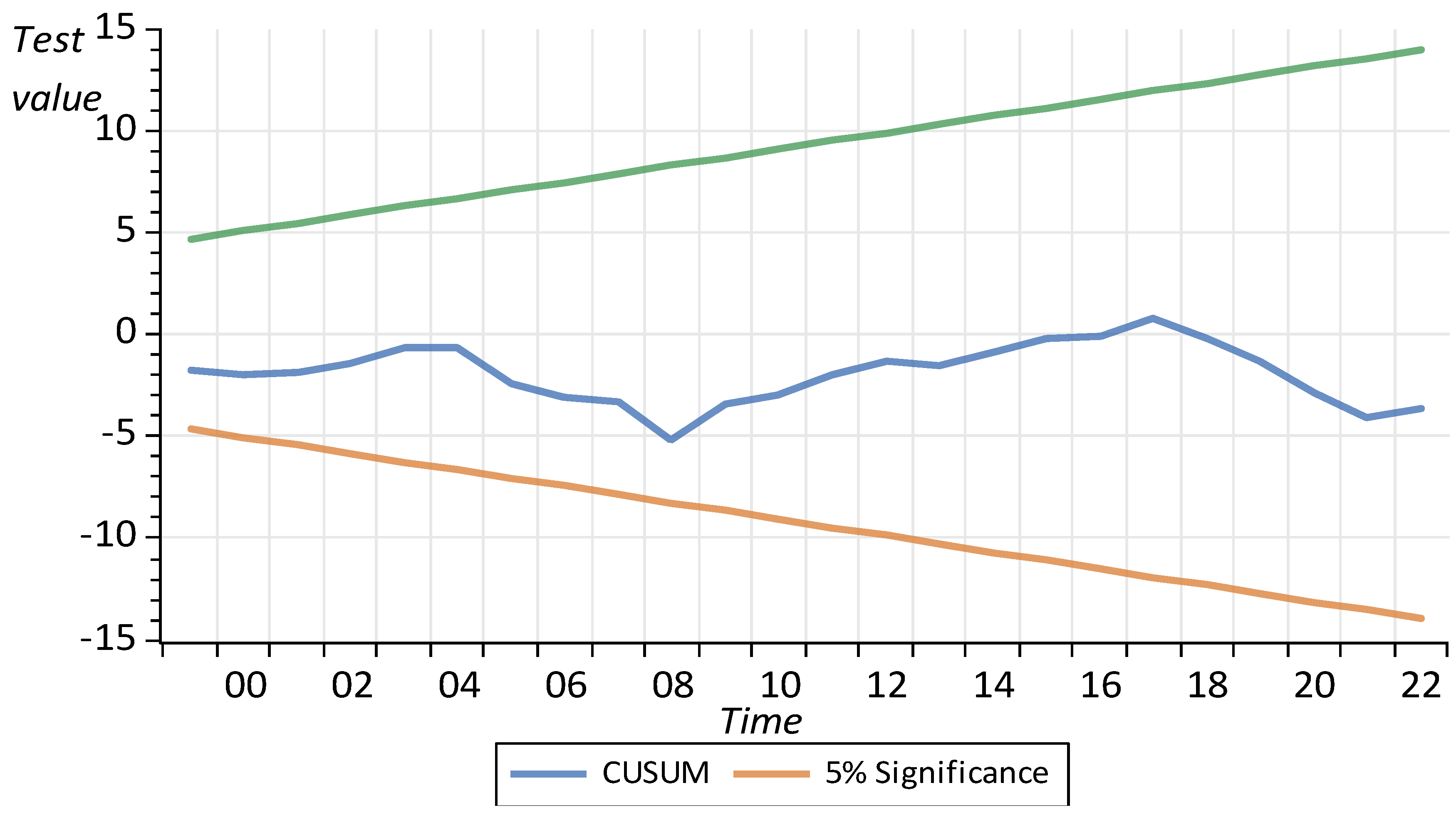
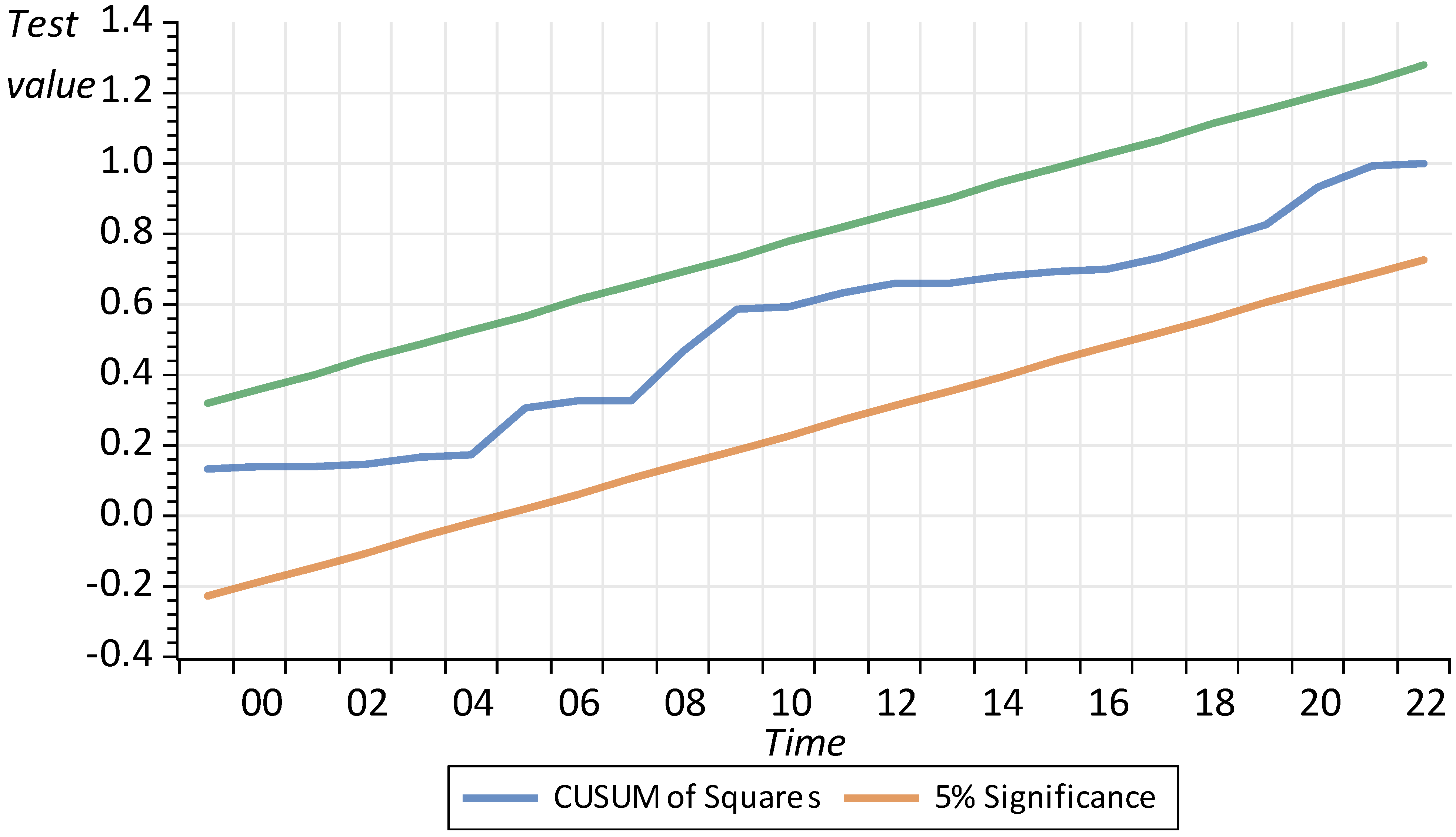
To evaluate the structural changes in the New Zealand economy, we employ the cumulative sum (CUSUM) and cumulative sum of squares (CUSUMSQ) tests developed by Brown et al. [59]. These tests assess the stability of both short- and long-run coefficients. Figure 4 and Figure 5 illustrate the CUSUM and CUSUMSQ test statistics for both models, which consistently fall within the critical bounds at the 5% significance level. This indicates that the estimated parameters remain stable over time, reinforcing the robustness of our statistical findings.

4.2. The ARDL Results for Life Expectancy Model

Table 5. The ARDL results for the impacts of different variables on life expectancy.

Short-Run Effect			Long-Run Effect
Variables	Coeff.	Std. Err. (Prob.)	Variables	Coeff.	Std. Err. (Prob.)
ECT(-1)	−0.147 *	0.015 (0.000)	LnLEXP(-1)	−0.147	0.166 (0.384)
D(LnLEXP(-1))	−0.661 *	0.097 (0.000)	LnTRAD(-1)	0.010	0.008 (0.252)
D(LnLEXP(-2))	−0.544 *	0.105 (0.000)	LnGFCF(-1)	0.004	0.005 (0.482)
D(LnTRAD)	0.019 *	0.005 (0.000)	LnHCON(-1)	0.005 **	0.002 (0.012)
D(LnTRAD(-1))	0.010 **	0.005 (0.043)	LnURB	0.427 **	0.192 (0.035)
D(LnGFCF)	−0.004	0.004 (0.240)	LnHEXP(-1)	0.019	0.017 (0.266)
D(LnGFCF(-1))	−0.015 *	0.003 (0.000)	LnREC(-1)	0.028 *	0.010 (0.010)
D(LnHCON)	0.002 *	0.000 (0.000)	LnTRCO2(-1)	−0.069 *	0.019 (0.001)
D(LnHCON(-1))	−0.003 *	0.001 (0.000)	C	−0.460	0.948 (0.632)
D(LnHCON(-2))	−0.002 *	0.001 (0.003)
D(LnHEXP)	0.046 *	0.013 (0.001)
D(LnREC)	0.018 **	0.007 (0.017)
D(LnREC(-1))	0.014 **	0.006 (0.020)
D(LnTRCO2)	−0.053 *	0.012 (0.000)
D(LnTRCO2(-1))	0.036 *	0.012 (0.007)
Statistics	Value	Prob.	Statistics	Value
F-statistic	4.202	(0.001)	Adjusted R2	0.787
D-W stat	1.880

Note: * p < 0.01, ** p < 0.05.

presents the dynamic ARDL simulation results for model 1, illustrating the effects of the various variables on life expectancy in New Zealand. The findings reveal that while trade has a positive relationship with life expectancy in the short term, its long-term relationship is positive yet insignificant. Specifically, a 1% increase in trade may correlate with a 0.02% rise in life expectancy in the short run. This suggests that increased trade activities may enhance household welfare, leading to improved life expectancy. Given the limited research on the relationship between trade and life expectancy, we draw on GDP as an alternative variable to support our findings, as trade is one of the main components of GDP calculation. These results align with the existing literature, including the study by Murthy et al. [15], which demonstrates a positive relationship between economic growth and life expectancy in D-8 countries; Shaari et al. [50] reached a similar conclusion.

Gross fixed capital formation, which means saving and investment in infrastructure, has a positive and insignificant relationship with life expectancy in the long run, but it has a negative and still insignificant impact in the short run. Household expenditure may have a positive impact on life expectancy in the long run, suggesting that a 1% increase in household expenditures is associated with a 0.005% increase in life expectancy. It may also have a short-term positive impact on life expectancy, although of a smaller magnitude (0.002). Given that consumption is the primary component of the household’s utility function, an increase in household expenditure on goods and services indicates that households want to improve their welfare assuming inflation remains constant.

Public health expenditures emerge as a significant factor that can positively influence life expectancy. As illustrated in Table 5, these expenditures yield beneficial effects in both the short and long term; however, the long-run coefficient lacks statistical significance. Specifically, the short-run coefficient of public health expenditure is 0.046, indicating that a 1% increase in public health spending is associated with a 0.05% rise in life expectancy within the nation. These findings align with the research conducted by Murthy et al. [15] concerning D-8 countries. Furthermore, studies by Owusu et al. [60] and Ahmad et al. [29] support the notion that enhanced health expenditure contributes to increased life expectancy.

The findings indicate that urbanisation influences life expectancy primarily over the long term, with a clear positive relationship between the two. It suggests that a 1% rise in urbanisation is associated with a 0.43% increase in life expectancy in the long run. As urban areas expand, they offer enhanced facilities, including diverse educational opportunities at all levels, high-quality transportation systems, professional healthcare services, and various recreational spaces like parks. These improvements significantly boost overall welfare and longevity. This aligns with the study by Mahalik et al. [16], which confirmed that urbanisation can positively impact life expectancy across developed, emerging, and developing nations. Additionally, Tripathi and Maiti [30] emphasised that sustainable urbanisation, when effectively managed, can lead to improved health outcomes.

Two other crucial factors influencing life expectancy are renewable energy consumption and transport-related CO₂ emissions. The ARDL analysis presented in Table 5 reveals a positive relationship between renewable energy consumption and life expectancy, both in the short and long run. Specifically, a 1% increase in renewable energy consumption correlates with a 0.03% increase in life expectancy over the long run and a 0.02% increase in the short run. These findings are consistent with research conducted by Guo et al. [49] and Shaari et al. [50], which also identifies the positive effects of renewable energy consumption on life expectancy.

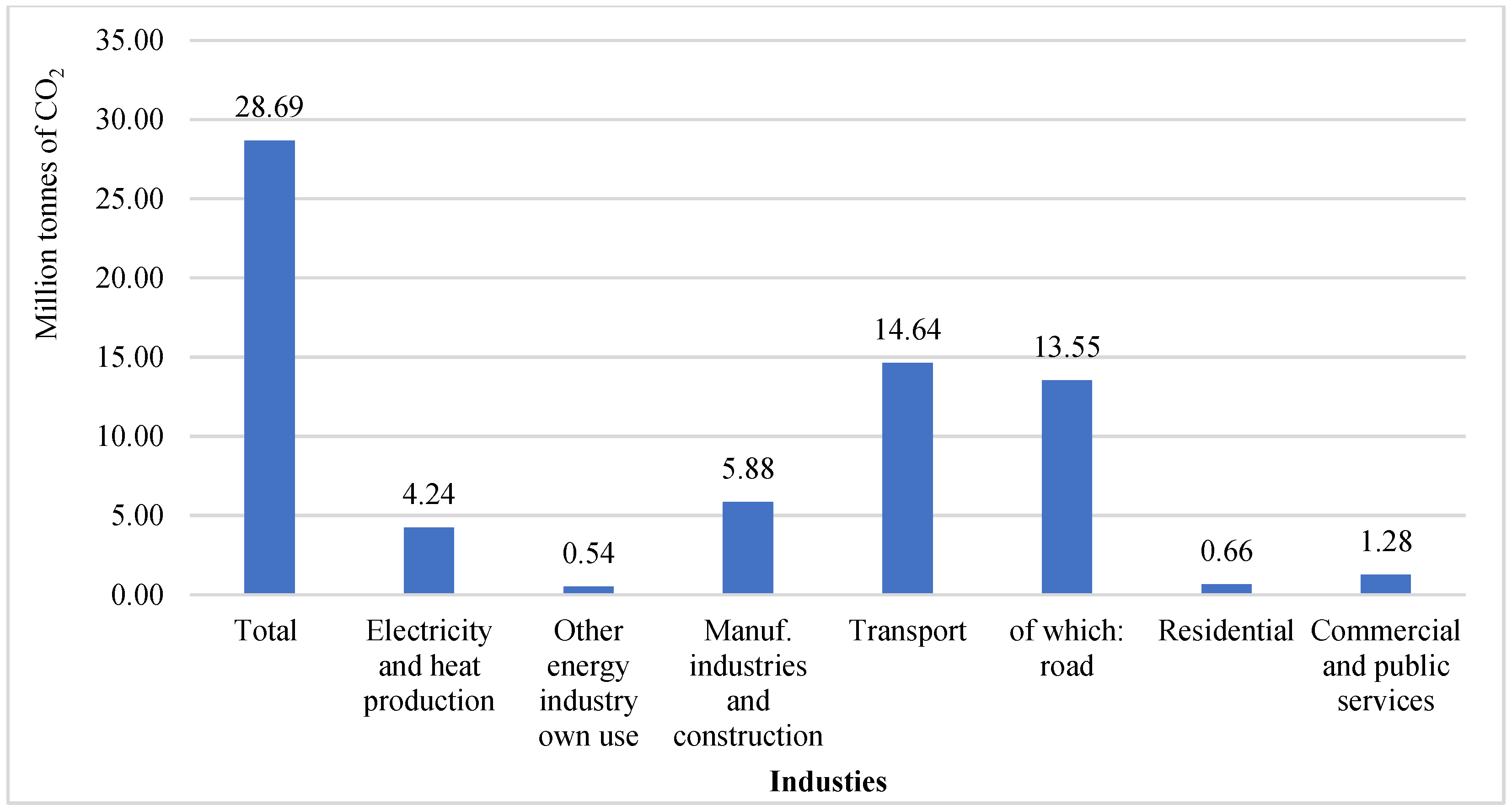
Transport-related CO₂ emissions, as highlighted in the introduction, influence life expectancy and mortality by generating air pollutants and toxic gases. Consequently, their impact is indirect. Transport CO₂ emissions can diminish life expectancy, both in the short and long term. Specifically, a 1% increase in transport CO₂ emissions correlates with a decrease in life expectancy of 0.07% in the long run and 0.05% in the short run. This issue primarily arises from the reliance on non-clean fuels, such as fossil fuels, which significantly increase emissions in the environment. Living in areas with high air pollution and toxic gases exacerbates health issues for households, resulting in increased healthcare expenditures. Consequently, households will have less disposable income for leisure and other activities, leading to a decline in their welfare and life expectancy.

Research by Emodi et al. [48] and Osabohien et al. [45] supports these findings, demonstrating the adverse effects of CO₂ emissions on life expectancy across various countries. Similarly, Mahalik et al. [16] identified a negative correlation between CO₂ emissions and life expectancy in a study encompassing 65 countries. However, Das and Debanth [44] reported that CO₂ emissions are not associated with an adverse effect on life expectancy in India.

The coefficient of the error correction term (ECT(-1)) has a negative sign and is statistically significant. The analysis indicates that 15% of error correction takes place annually, moving towards long-run equilibrium, as evidenced by the negative and highly significant nature of the error correction term (ECT). This confirms a causal relationship between trade, gross fixed capital formation, household expenditure, public health expenditure, renewable energy consumption, and transport CO₂ emissions with life expectancy.

Table 6. The dynamic ARDL simulations results for the impacts of different variables on life expectancy.

Short-Run Effect			Long-Run Effect
Variables	Coeff.	Std. Err. (Prob.)	Variables	Coeff.	Std. Err. (Prob.)
L1_LnLEXP	−0.485 *	0.139 (0.001)	D_LnTRAD	0.008	0.008 (0.333)
L1_LnTRAD	0.012	0.010 (0.252)	D_LnGFCF	0.009	0.006 (0.147)
L1_LnGFCF	0.011 **	0.005 (0.041)	D_LnHCON	0.001 ***	0.001 (0.080)
L1_LnHCON	0.002 **	0.001 (0.033)	D_LnURB	0.927	1.070 (0.392)
L1_LnURB	0.382 *	0.105 (0.001)	D_LnHEXP	0.024	0.023 (0.292)
L1_LnHEXP	0.043 *	0.015 (0.009)	D_LnREC	0.002	0.011 (0.831)
L1_LnREC	0.014 ***	0.007 (0.055)	D_LnTRCO2	0.002	0.017 (0.929)
L1_LnTRCO2	−0.003	0.015 (0.859)
Statistics	Value	(Prob.)	Statistics
Adjusted R2	0.442		Adjusted R2
F-statistic (15, 35)	3.64	(0.001)

Note: * p < 0.01, ** p < 0.05, *** p < 0.1.

showcases the results from the dynamic ARDL simulation method, supporting the findings presented in Table 5. This model has been developed to assess the influence of shocks in renewable energy consumption and transport-related CO₂ emissions on life expectancy. The simulation outcomes indicate that a 1% rise in public health expenditure and renewable energy consumption can be associated with increases in life expectancy of approximately 0.04% and 0.01% in the long run, respectively. However, the short-term effects of these variables are not statistically significant.

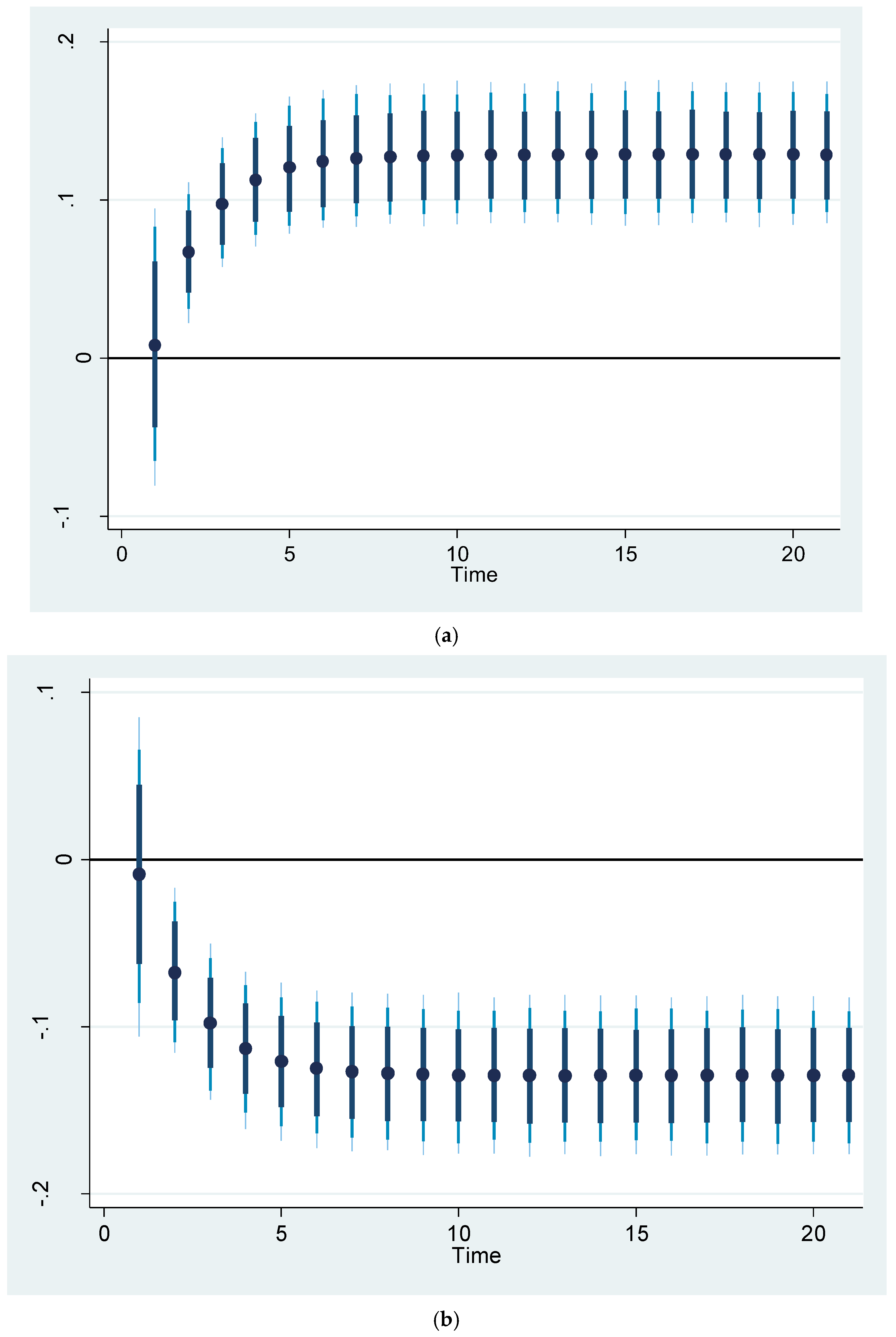
We employed the dynamic ARDL simulation model to simulate the long-run effects of a 5% change (increase and decrease) in renewable energy consumption and transport CO₂ emissions on life expectancy. The results of these simulations are presented in Figure 6 and Figure 7. Figure 6 shows the impact of a 5% increase and decrease in renewable energy consumption on life expectancy. It shows that increasing or decreasing renewable energy consumption by 5% can be associated with a corresponding increase or decrease in life expectancy of approximately 1.2%. It should be noted that the shock at the first stage may either increase or decrease the life expectancy, depending on the circumstances. The values are higher than the coefficients of this variable in Table 5 and Table 6 because of the magnitude of the shock inflicted on this variable. In Figure 6, the black dot (●) represents the predicted life expectancy resulting from a 5% shock in renewable energy consumption in a log-log model. The dark, light blue, and dark blue spikes indicate 75%, 90%, and 95% confidence intervals, respectively.

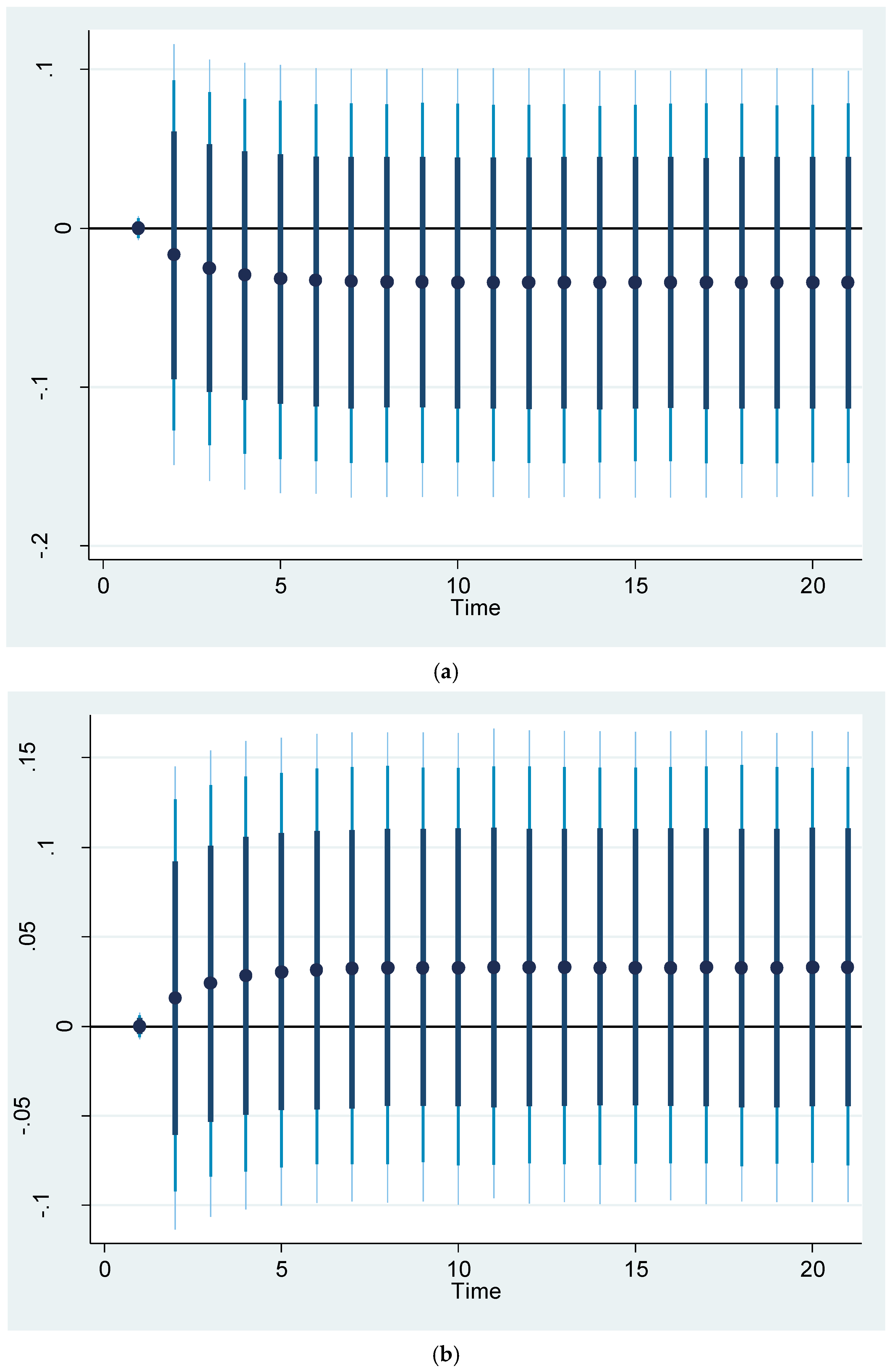
The simulation model presented in Figure 7 shows the effects of a 5% increase and decrease in transport CO₂ emissions on life expectancy. The findings show that a 5% increase or decrease in CO₂ emissions from the transportation sector is expected to result in a decrease or increase in New Zealanders’ life expectancy of nearly 0.04%, respectively. It is worth noting that the shock at the first stage may not change the life expectancy. The values are greater than the coefficient of this variable in Table 5 and Table 6 in the long run. This is because of the magnitude of the shock that affected life expectancy. The impact of renewable energy consumption on life expectancy is greater than the transport CO₂ emissions because it includes all renewable energy sources.

4.3. The ARDL Results for the Mortality Model

Table 7. Results of the ARDL model for the impacts of different variables on mortality.

Short-Run Effect			Long-Run Effect
Variables	Coeff.	Std. Err. (Prob.)	Variables	Coeff.	Std. Err. (Prob.)
ECT(-1)	−0.368 *	0.051 (0.000)	LnMORT(-1)	−0.368	0.391 (0.367)
D(LnMORT(-1))	−0.658 *	0.168 (0.001)	LnTRAD(-1)	−0.590 **	0.197 (0.012)
D(LnMORT(-2))	−0.857 *	0.220 (0.001)	LnGFCF(-1)	−0.210 ***	0.115 (0.095)
D(LnTRAD)	−0.197 *	0.048 (0.001)	LnHCON(-1)	−0.036	0.030 (0.253)
D(LnTRAD(-1))	0.170 *	0.056 (0.007)	LnURB(-1)	−16.746 **	5.740 (0.014)
D(LnGFCF)	−0.036	0.036 (0.330)	LnHEXP(-1)	−0.524 **	0.185 (0.016)
D(LnGFCF(-1))	0.258 *	0.048 (0.000)	LnREC(-1)	−0.657 ***	0.315 (0.061)
D(LnHCON)	−0.004	0.004 (0.254)	LnTRCO2(-1)	1.605 **	0.548 (0.014)
D(LnHCON(-1))	0.024 *	0.006 (0.001)	C	61.082 **	23.681 (0.026)
D(LnHEXP)	−0.065	0.076 (0.407)
D(LnHEXP(-1))	−0.054	0.068 (0.436)
D(LnREC)	−0.426 **	0.104 (0.001)
D(LnREC(-1))	0.283 **	0.127 (0.039)
D(LnTRCO2)	0.287 **	0.117 (0.024)
D(LnTRCO2(-1))	−0.920 *	0.168 (0.000)
Statistics	Value	Prob.
Adjusted R2	0.753		D-W stat	2.290
F-statistic	6.206	0.000

Note: * p < 0.01, ** p < 0.05, *** p < 0.1.

reports the estimated results of the ARDL model for mortality (model 2). It shows the short- and long-run impacts of trade, gross fixed capital formation, household expenditure, government health expenditures, urbanisation, renewable energy consumption, and transport CO₂ emissions on mortality in New Zealand. The results indicate that trade has a negative and statistically significant correlation with mortality in both the short and long run. This means that a 1% increase in trade can reduce mortality by 0.59% in the long run and 0.20% in the short run. Trade not only enriches the economy and boosts household incomes, but it also enhances access to essential medicines and health-related resources. This reduces poverty levels and improves overall welfare. Mejia [61] found that trade can have a negative but insignificant impact on mortality. Byaro et al. [62] also found that more trade contributes to health improvement and a decline in the mortality rate.

The long-term coefficient for gross fixed capital formation is not only negative but also statistically significant, indicating that increased investment, particularly in public infrastructure and healthcare facilities, such as clean water, sanitation, and transportation systems, can substantially reduce mortality rates [42]. Berman et al. [41] demonstrated that in low-income countries, investing in healthcare infrastructure is significantly associated with reductions in maternal and child mortality rates. These findings are also supported by the research by Eboh et al. [63], who found that gross fixed capital formation can have a positive and significant impact on under-five child mortality. In contrast, research conducted by Sial et al. [64] and Kiross et al. [65] highlighted the negative relationship between capital formation and mortality.

Household expenditure has a negligible and statistically insignificant effect on mortality in both the short and long run. This suggests that while increases in household spending may correlate with decreases in mortality during these periods, the relationship is not strong enough to be considered meaningful. Increased household spending on high-quality food, leisure activities, and medical care does not necessarily result in lower overall mortality rates, particularly among adults. This is due to significant factors such as car accidents and various types of cancer, which are prevalent in New Zealand and other countries.

The urbanisation variable may also have a negative and statistically significant impact on mortality in the long run, but not in the short run. Because of the high accessibility to facilities and healthcare centres in cities, urbanisation can have a negative impact on mortality. Similar results were obtained by Guo et al. [49], showing that urbanisation can reduce infant mortality in SAARC countries. Tripathi and Maiti [30] showed that well-managed urbanisation can be beneficial for achieving higher health outcomes. However, high-density urbanisation may increase mortality [66].

Another variable that may have a negative impact on mortality is public health expenditures. The results in Table 7 show that public health expenditure has a negative correlation with mortality in both the short and long run, but the short-run coefficient is not statistically significant. The long-run coefficient of public health expenditure is −0.524, indicating that a 1% increase in public health expenditure is associated with a 0.52% decline in mortality. Khatri et al. [54] pointed out that economic growth and health expenditure can help reduce child mortality in Nepal. Owusu et al. [60] and Onofrei et al. [67] also found a negative relationship between health expenditure and mortality.

Renewable energy consumption and CO₂ emissions from transportation are two other important factors that may influence mortality. The results presented in Table 7 indicate that renewable energy consumption may lead to reduced mortality rates in both the short and long run. This variable shows that living in an environment with lower air pollution can reduce the risk of disease-related air quality issues. Statistics reveal that approximately 43% of New Zealand’s total energy supply in 2023 was derived from renewable energy sources, such as geothermal and hydropower [68]. Similar results were obtained by Guo et al. [49], showing that renewable energy consumption can reduce infant mortality in SAARC countries. Byaro and Rwezaula [34] and Koengkan et al. [69] also found similar results in their study for 26 sub-Saharan African countries.

In contrast, transport CO₂ emissions may have a positive and statistically significant impact on mortality in both the long and short run. The findings reveal that a 1% rise in transport CO₂ emissions is associated with a 1.6% increase in mortality over the long term and a 0.29% increase in the short term. These results support the results of the studies conducted by Guo et al. [49], Erdogan et al. [13], and Adeleye et al. [52], suggesting that a positive correlation between CO₂ emissions and mortality. Emodi et al. [48] also showed that transport CO₂ emissions may increase the number of deaths in developing countries.

The coefficient of the error correction term (ECT(-1)) has a negative sign and is statistically significant. It shows the rate of short-run adjustment towards the long-run equilibrium in the event of an equilibrium deviation.

Table 8. The dynamic ARDL simulations results for the impacts of different variables on mortality.

Long-Run Effect			Short-Run Effect
Variables	Coeff.	Std. Err. (Prob.)	Variables	Coeff.	Std. Err. (Prob.)
L1_LnMORT	−0.230 **	0.099 (0.027)	D_LnTRAD	−0.143 *	0.052 (0.009)
L1_LnTRAD	−0.177 *	0.060 (0.006)	D_LnGFCF	−0.004	0.039 (0.919)
L1_LnGFCF	−0.046	0.030 (0.139)	D_LnHCON	−0.005	0.005 (0.342)
L1_LnHCON	−0.014 **	0.006 (0.022)	D_LnURB	−14.750 **	6.412 (0.028)
L1_LnURB	0.705	0.436 (0.115)	D_LnHEXP	−0.322 **	0.134 (0.022)
L1_LnHEXP	−0.157 **	0.077 (0.050)	D_LnREC	0.046	0.067 (0.498)
L1_LnREC	−0.124 *	0.045 (0.010)	D_LnTRCO2	−0.220 **	0.100 (0.035)
L1_LnTRCO2	0.044	0.092 (0.636)
Statistics	Value	Prob.
Adjusted R2	0.563
F-statistic	5.30	(0.000)

Note: * p < 0.01, ** p < 0.05.

presents the results of the dynamic ARDL simulation method. The results support the findings of the ARDL model presented in Table 7. This model is estimated to simulate the effects of a shock on renewable energy consumption, transport CO₂ emissions, and mortality.

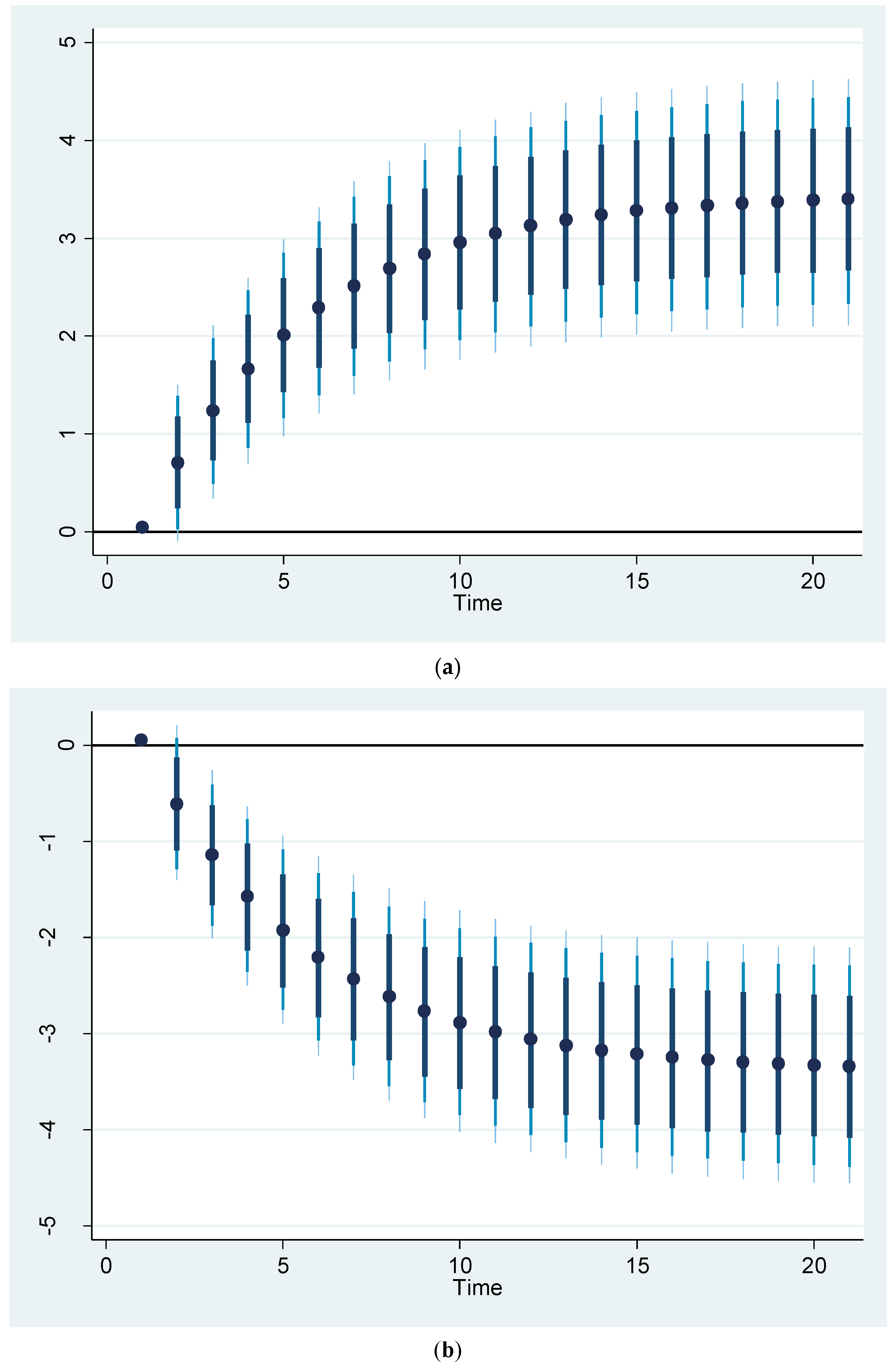
The dynamic ARDL simulation model simulates the long-term effects of a 5% change (increase and decrease) in renewable energy consumption and transport CO₂ emissions on mortality. The results of these simulations are presented in Figure 8 and Figure 9. Figure 8 illustrates the effect of a 5% increase and decrease in renewable energy consumption on mortality. The findings indicate that a 5% increase or decrease in renewable energy consumption is expected to be associated with a nearly 2% decrease or increase in mortality rates among New Zealanders. It should be noted that the shock at the first stage may increase or decrease the mortality rate, depending on the circumstances. The values exceed the coefficients for this variable presented in Table 7 and Table 8, owing to the intensity of the shock applied to it.

The simulation results illustrated in Figure 9 demonstrate how a 5% variation—either an increase or decrease—in transport CO₂ emissions may impact mortality rates. The findings reveal a significant correlation: a 5% increase or decrease in CO₂ emissions from the transportation sector may correspond to a nearly 3.3% change in New Zealand’s mortality rate. It should be noted that the shock at the first stage may not affect the mortality rate. In the long run, the values are greater than the coefficient of this variable in Table 7 and Table 8. This is because of the magnitude of the shock that affected mortality.

5. Conclusions

This study investigated the impacts of trade, gross fixed capital formation, household expenditures, government health expenditures, urbanisation, renewable energy consumption, and transport CO₂ emissions on two important societal well-being variables (i.e., life expectancy and mortality) in New Zealand using the dynamic autoregressive distributed lag simulations methodology during 1972–2022.

The study’s findings show that household expenditure and renewable energy consumption can contribute to increased life expectancy in both the short and long term, although the magnitude of the impact may be smaller in the short term. In the long run, urbanisation also may have a positive and statistically significant effect on life expectancy. In the long run, a 1% increase in household expenditure, urbanisation, and renewable energy consumption is associated with increases in life expectancy of 0.005%, 0.43%, and 0.03%, respectively. Conversely, transport CO₂ emissions may negatively influence life expectancy in both time frames; a 1% increase in emissions may reduce life expectancy by 0.07% in the short run and by 0.05% in the long run.

The simulation results show that if the consumption of renewable energy increases or decreases by 5%, is likely to result in a 1.2% increase or decrease in the life expectancy of New Zealanders, respectively. The results also show that if the CO₂ emissions from the transport sector increase or decrease by 5%, the life expectancy of New Zealanders may decrease or increase by nearly 0.05%, respectively.

The mortality results reveal that most variables in the model are statistically significant in the long run. This, along with life expectancy results, emphasises that while mortality acts as a reliable long-run indicator, life expectancy tends to be more focused on short-run trends. Urbanisation emerges as a primary factor in reducing mortality. Additional results demonstrate that trade, gross fixed capital formation, public health expenditure, and renewable energy consumption all exhibit a negative and statistically significant relationship with mortality. Furthermore, transport CO₂ emissions have an indirect relationship with mortality in both the short and long term, increasing by 1.6% and 0.29% for each corresponding 1% rise.

The simulation results of the predicted impact of renewable energy consumption on mortality show that a 5% increase or decrease in renewable energy consumption may result in a 2% increase or decrease in mortality among New Zealanders, respectively. The results show that if CO₂ emissions from the transport sector increase or decrease by 5%, the mortality rate of New Zealanders may increase or decrease by around 3.3%, respectively.

As air pollutants and toxic gases from transportation and industry negatively affect life expectancy and mortality, it is recommended that the use of renewable energy sources in the transport sector increases, as well as the use of environmentally friendly infrastructure, machinery, and equipment in industries and services in the economy, to improve the social and health conditions of people in the country. It is essential to refrain from implementing policies that adversely affect household incomes and consumption, as well as the environment, as these can further exacerbate people’s health-related issues. Establishing stable healthcare expenditure policies is essential. Policymakers must consider the influence of other economic factors, such as trade dynamics, capital formation, and household consumption, when developing strategies aimed at enhancing public health outcomes.

The main limitation of this study lies in its inability to evaluate the effects of all relevant variables that affect the dependent variables—life expectancy and mortality—because these factors are highly influenced by human behaviour and lifestyle choices. Therefore, the observed correlations may be influenced by confounding variables that are not included in the model. Another limitation of the study is that we were not able to collect data on other major air pollutants, such as particulate matter, to investigate their effects on mortality and life expectancy.

References

1. Solaymani, S. CO2 emissions and the transport sector in Malaysia. Front. Environ. Sci. 2022, 9, 774164. [Google Scholar] [CrossRef]
2. United Nations Environmental Programme (UNEP). Pollution Action Note—Data You Need to Know; United Nations Environmental Programme (UNEP): Nairobi, Kenya, 2021; Available online: https://www.unep.org/interactives/air-pollution-note/ (accessed on 3 April 2025).
3. Ministry of Environment. New Zealand’s Greenhouse Gas Inventory 1990–2022: Snapshot; Ministry of Environment: Wellington, New Zealand, 2024. Available online: https://environment.govt.nz/assets/publications/GHG-inventory-2024-Snapshot.pdf (accessed on 20 March 2025).
4. International Energy Agency (IEA). Greenhouse Gas Emissions from Energy; International Energy Agency: Paris, France, 2024. [Google Scholar]
5. International Energy Agency (IEA). World Energy Balances: Highlights; International Energy Agency: Paris, France, 2024. [Google Scholar]
6. Solaymani, S.; Kardooni, R.; Yusoff, S.B.; Kari, F. The impacts of climate change policies on the transportation sector. Energy 2015, 81, 719–728. [Google Scholar] [CrossRef]
7. Solaymani, S. Which government supports are beneficial for the transportation subsectors. Energy 2021, 235, 121349. [Google Scholar] [CrossRef]
8. Solaymani, S.; Kari, F.; Zakaria, R.H. Evaluating the role of subsidy reform in addressing poverty levels in Malaysia: A CGE poverty framework. J. Dev. Stud. 2014, 50, 556–569. [Google Scholar] [CrossRef]
9. Lu, Q.; Fang, H.; Hou, J. The impact of energy supply side on the diffusion of low-carbon transformation on energy demand side under low-carbon policies in China. Energy 2024, 307, 132817. [Google Scholar] [CrossRef]
10. Chaabouni, S.; Saidi, K. The dynamic links between carbon dioxide (CO2) emissions, health spending and GDP growth: A case study for 51 countries. Environ. Res. 2017, 158, 137–144. [Google Scholar] [CrossRef]
11. Mohmmed, A.; Li, Z.; Arowolo, A.O.; Su, H.; Deng, X.; Najmuddin, O.; Zhang, Y. Driving factors of CO2 emissions and nexus with economic growth, development and human health in the Top Ten emitting countries. Resour. Conserv. Recycl. 2019, 148, 157–169. [Google Scholar] [CrossRef]
12. Ministry of Transport. Workstream 3 Environmental Outcomes; Working draft vD; Ministry of Transport: Wellington, New Zealand, 2020. Available online: https://www.transport.govt.nz/assets/Uploads/Paper/EnvironmentalOutcomes.pdf (accessed on 13 March 2025).
13. Erdogan, S.; Yildirm, D.C.; Gedikli, A. The Relationship Between CO2 Emissions and Health Indicators: The Case of Turkey. Econom. Lett. 2019, 6, 28–39. [Google Scholar]
14. Chatterjee, N.; Chatterjee, T.; Nath, A.; Koley, B. Life Expectancy Amid Higher Carbon Emissions: A Panel Data Analysis. In Climate Change and Regional Socio-Economic Systems in the Global South; Mishra, M., de Lucena, A.J., Maharaj, B., Eds.; Springer: Berlin/Heidelberg, 2024. [Google Scholar] [CrossRef]
15. Murthy, U.; Shaari, M.S.; Mariadas, P.A.; Abidin, N.Z. The Relationships between CO2 Emissions, Economic Growth and Life Expectancy. J. Asian Financ. Econ. Bus. 2021, 8, 801–808. [Google Scholar] [CrossRef]
16. Mahalik, M.K.; Le, T.; Le, H.; Mallick, H. How do sources of carbon dioxide emissions affect life expectancy? Insights from 68 developing and emerging economies. World Dev. Sustain. 2021, 1, 100003. [Google Scholar] [CrossRef]
17. Statistics New Zealand. Births, Deaths, and Selected Rates 2007–2023; Statistics New Zealand: Wellington, New Zealand, 2024. Available online: https://www.stats.govt.nz/topics/births-and-deaths/ (accessed on 10 April 2024).
18. Solaymani, S. Biodiesel and its potential to mitigate transport-related CO2 emissions. Carbon Res. 2023, 2, 38. [Google Scholar] [CrossRef]
19. Pahlavani, M.; Wilson, E.; Worthington, A.C. Trade-GDP Nexus in Iran: An Application of the Autoregressive Distributed Lag (ARDL) Model. Am. J. Appl. Sci. 2005, 2, 1158–1165. [Google Scholar] [CrossRef]
20. Kripfganz, S.; Schneider, D.C. ARDL: Estimating autoregressive distributed lag and equilibrium correction models. Stata J. 2023, 23, 983–1019. [Google Scholar] [CrossRef]
21. Reidpath, D.D.; Allotey, P. Infant mortality rate as an indicator of population health. J. Epidemiol. Community Health 2003, 57, 344–346. [Google Scholar] [CrossRef]
22. Miladinov, G. Socioeconomic development and life expectancy relationship: Evidence from the EU accession candidate countries. Genus 2020, 76, 2. [Google Scholar] [CrossRef]
23. Kocot, E.; Denkowska, S.; Fijorek, K. Are Measures of Health Status for the Total Population Good Proxies for the Health of the Older Population in International Comparison Studies? Int. J. Environ. Res. Public Health 2022, 19, 7559. [Google Scholar] [CrossRef] [PubMed]
24. Lelieveld, J.; Evans, J.S.; Fnais, M.; Giannadaki, D.; Pozzer, A. The contribution of outdoor air pollution sources to premature mortality on a global scale. Nature 2015, 525, 367–371. [Google Scholar] [CrossRef]
25. Burnett, R.; Chen, H.; Szyszkowicz, M.; Fann, N.; Hubbell, B.; Pope, C.A., 3rd; Apte, J.S.; Brauer, M.; Cohen, A.; Weichenthal, S.; et al. Global estimates of mortality associated with long-term exposure to outdoor fine particulate matter. Proc. Natl. Acad. Sci. USA 2018, 15, 9592–9597. [Google Scholar] [CrossRef]
26. Bayraktar, O.M.; Mutlu, A. Analyses of industrial air pollution and long-term health risk using different dispersion models and WRF physics parameters. Air Qual. Atmos. Health 2024, 17, 2277–2305. [Google Scholar] [CrossRef]
27. Zhao, Q.; Guo, Y.; Ye, T.; Gasparrini, A.; Tong, S.; Overcenco, A.; Urban, A.; Schneider, A.; Entezari, A.; Zanobetti, A.; et al. Global, regional, and national burden of mortality associated with non-optimal ambient temperatures from 2000 to 2019: A three-stage modelling study. Lancet Planet. Health 2021, 5, e415–e425. [Google Scholar] [CrossRef]
28. Vlahov, D.; Galea, S.; Gibble, E.; Freudenberg, N. Urban as a Determinant of Health. J. Urban Health 2007, 84, 16–26. [Google Scholar] [CrossRef] [PubMed]
29. Ahmad, N.; Raid, M.; Alzyadat, J.; Alhawal, H. Impact of urbanization and income inequality on life expectancy of male and female in South Asian countries: A moderating role of health expenditures. Humanit. Soc. Sci. Commun. 2023, 10, 552. [Google Scholar] [CrossRef]
30. Tripathi, S.; Maiti, M. Does urbanization improve health outcomes: A cross country level analysis. Asia-Pac. J. Reg. Sci. 2023, 7, 277–316. [Google Scholar] [CrossRef]
31. Liu, H.; Zhong, K. Relationship between health spending, life expectancy and renewable energy in China: A new evidence from the VECM approach. Front. Public Health 2022, 20, 993546. [Google Scholar] [CrossRef]
32. Polcyn, J.; Voumik, L.C.; Ridwan, M.; Ray, S.; Vovk, V. Evaluating the Influences of Health Expenditure, Energy Consumption, and Environmental Pollution on Life Expectancy in Asia. Int. J. Environ. Res. Public Health 2022, 20, 4000. [Google Scholar] [CrossRef]
33. Abdulganiyu, S.; Tijjani, M. Healthcare Expenditure and Life Expectancy in Africa: A Panel Study. South Asian J. Soc. Stud. Econ. 2021, 9, 1–9. [Google Scholar] [CrossRef]
34. Byaro, M.; Rwezaula, A. The health impacts of renewable energy consumption in sub-Saharan Africa: A machine learning perspective. Energy Strategy Rev. 2024, 57, 101621. [Google Scholar] [CrossRef]
35. Ibrahim, R.L.; Ajide, K.B. The role of income level and institutional quality in the non-renewable energy consumption and life expectancy nexus: Evidence from selected oil-producing economies in Africa. OPEC Energy Rev. 2021, 45, 341–364. [Google Scholar] [CrossRef]
36. Karimi Alavijeh, N.; Ahmadi Shadmehri, M.T.; Dehdar, F.; Zangoei, S.; Nazeer, N. The role of renewable energy on life expectancy: Evidence from method of moments quantile regression based on G-7 countries data. Int. J. Energy Sect. Manag. 2024, 18, 767–788. [Google Scholar] [CrossRef]
37. Vatamanu, A.F.; Onofrei, M.; Cigu, E.; Oprea, F. Renewable energy consumption, institutional quality and life expectancy in EU countries: A cointegration analysis. Energy Sustain. Soc. 2025, 15, 2. [Google Scholar] [CrossRef]
38. Cícero, V.C.; Corrêa Dias, L.C.; Zahran, S. Trade Liberalization and Mortality Rates: Evidence of Pro-Cyclical Mortality From Brazil. Health Econ. 2024, 34, 392. [Google Scholar] [CrossRef]
39. Shah, M.I.; Ullah, I.; Xingjian, X.; Haipeng, H.; Rehman, A.; Zeeshan, M.; Alam Afridi, F.E. Modeling Trade Openness and Life Expectancy in China. Risk Manag. Healthc. Policy 2021, 14, 1689–1701. [Google Scholar] [CrossRef] [PubMed]
40. Chen, Z.; Ma, Y.; Hua, J.; Wang, Y.; Guo, H. Impacts from Economic Development and Environmental Factors on Life Expectancy: A Comparative Study Based on Data from Both Developed and Developing Countries from 2004 to 2016. Int. J. Environ. Res. Public Health 2020, 18, 8559. [Google Scholar] [CrossRef]
41. Berman, A.N.; Biery, D.W.; Ginder, C.; Singh, A.; Baek, J.; Wadhera, R.K.; Wu, W.Y.; Divakaran, S.; DeFilippis, E.M.; Hainer, J.; et al. Association of Socioeconomic Disadvantage with Long-term Mortality After Myocardial Infarction: The Mass General Brigham YOUNG-MI Registry. JAMA Cardiol. 2021, 6, 880–888. [Google Scholar] [CrossRef]
42. Nikita, K.A.; Anatole, T.; Gildas, N.T. Infrastructure’s role in enhancing child well-being across sub-Saharan Africa. Sustain. Futures 2024, 8, 100270. [Google Scholar] [CrossRef]
43. Redzwan, N.; Ramli, R. Carbon Emissions, Health Expenditure, and Economic Effects on Life Expectancy in Malaysia. World 2024, 5, 588–602. [Google Scholar] [CrossRef]
44. Das, S.; Debanth, A. Impact of CO2 emission on life expectancy in India: An autoregressive distributive lag (ARDL) bound test approach. Futur. Bus. J. 2023, 9, 5. [Google Scholar] [CrossRef]
45. Osabohien, R.; Aderemi, T.A.; Akindele, D.B.; Jolayemi, L.B. Carbon Emissions and Life Expectancy in Nigeria. Int. J. Energy Econ. Policy 2020, 11, 497–501. Available online: https://www.econjournals.com.tr/index.php/ijeep/article/view/10834 (accessed on 3 April 2025). [CrossRef]
46. Rahman, M.M.; Alam, K. The nexus between health status and health expenditure, energy consumption and environmental pollution: Empirical evidence from SAARC-BIMSTEC regions. BMC Public Health 2021, 21, 1694. [Google Scholar] [CrossRef]
47. Mueller, N.; Rojas-Rueda, D.; Basagaña, X.; Cirach, M.; Cole-Hunter, T.; Dadvand, P.; Martinez, D. Urban and transport planning related exposures and mortality: A health impact assessment for cities Environ. Health Perspect. 2017, 125, 89–96. [Google Scholar] [CrossRef]
48. Emodi, N.V.; Inekwe, J.N.; Zakari, A. Transport infrastructure, CO2 emissions, mortality, and life expectancy in the Global South. Transp. Policy 2022, 128, 243–253. [Google Scholar] [CrossRef]
49. Guo, A.; Ullah, O.; Zeb, A.; Din, N.U.; Hussain, S. Unveiling health dynamics: Exploring the impact of CO2 emissions, urbanization, and renewable energy on life expectancy and infant mortality in SAARC countries (1990–2022). Nat. Resour. Forum 2024. [Google Scholar] [CrossRef]
50. Shaari, M.S.; Majekodunmi, T.B.; Sulong, A.; Esquivias, W.S. Examining the interplay between green technology, CO2 emissions, and life expectancy in the ASEAN-5 countries: Insights from the panel FMOLS and DOLS approaches. Discov. Sustain. 2024, 5, 456. [Google Scholar] [CrossRef]
51. Sinha, A. Carbon Emissions and Mortality Rates: A Causal Analysis for India (1971–2010). Int. J. Econ. Pract. Theor. 2014, 4, 486–492. [Google Scholar]
52. Adeleye, B.N.; Olohunlana, A.O.; Ibukun, C.O.; Soremi, T.; Suleiman, B. Mortality rate, carbon emissions, renewable energy and per capita income nexus in Sub-Saharan Africa. PLoS ONE 2022, 17, e0274447. [Google Scholar] [CrossRef]
53. Rasoulinezhad, E.; Taghizadeh-Hesary, F.; Taghizadeh-Hesary, F. How Is Mortality Affected by Fossil Fuel Consumption, CO2 Emissions and Economic Factors in CIS Region? Energies 2019, 13, 2255. [Google Scholar] [CrossRef]
54. Khatri, B.B.; Poudel, O.; Timsina, T.R.; Sapkota, K.N. Effects of Carbon Dioxide Emissions on Child Mortality in Nepal. Int. J. Energy Econ. Policy 2024, 15, 566–577. [Google Scholar] [CrossRef]
55. Pesaran, M.H.; Shin, Y.; Smith, R.J. Bounds testing approaches to the analysis of level relationships. J. Appl. Econom. 2001, 16, 289–326. [Google Scholar] [CrossRef]
56. Abbasi, K.R.; Shahbaz, M.; Jiao, Z.; Tufail, M. How energy consumption, industrial growth, urbanization, and CO2 emissions affect economic growth in Pakistan? A novel dynamic ARDL simulations approach. Energy 2021, 221, 119793. [Google Scholar] [CrossRef]
57. Jordan, S.; Philips, A.Q. Cointegration Testing and Dynamic Simulations of Autoregressive Distributed Lag Models. Stata J. 2018, 18, 902–923. [Google Scholar] [CrossRef]
58. Sarkodie, S.A.; Strezov, V.; Weldekidan, H.; Asamoah, E.F.; Owusu, P.A.; Doyi, I.N.Y. Environmental sustainability assessment using dynamic Autoregressive-Distributed Lag simulations—Nexus between greenhouse gas emissions, biomass energy, food and economic growth. Sci. Total Environ. 2019, 668, 318–332. [Google Scholar] [CrossRef] [PubMed]
59. Brown, R.L.; Durbin, J.; Evans, J.M. Techniques for Testing the Constancy of Regression Relationships over Time. J. R. Stat. Soc. Ser. B 1975, 37, 149–163. [Google Scholar] [CrossRef]
60. Owusu, P.A.; Sarkodie, S.A.; Pedersen, P.A. Relationship between mortality and health care expenditure: Sustainable assessment of health care system. PLoS ONE 2021, 16, e0247413. [Google Scholar] [CrossRef] [PubMed]
61. Mejia, S.A. Globalization, foreign direct investment, and child mortality: A cross-national analysis of less-developed countries, 1990–2019. Int. J. Comp. Sociol. 2023, 65, 378–406. [Google Scholar] [CrossRef]
62. Byaro, M.; Nkonoki, J.; Mayaya, H. The contribution of trade openness to health outcomes in sub-Saharan African countries: A dynamic panel analysis. Res. Glob. 2021, 3, 100067. [Google Scholar] [CrossRef]
63. Eboh, I.A.; Aduku, E.B.; Onwughalu, U.B. Health Expenditure, Child Mortality and Economic Growth in Nigeria. Int. J. Econ. Dev. Res. (IJEDR) 2022, 3, 198–216. [Google Scholar] [CrossRef]
64. Sial, M.H.; Arshed, N.; Amjad, M.A.; Khan, Y.A. Nexus between fossil fuel consumption and infant mortality rate: A non-linear analysis. Environ. Sci. Pollut. Res. 2022, 29, 58378–58387. [Google Scholar] [CrossRef]
65. Kiross, G.T.; Chojenta, C.; Barker, D.; Loxton, D. The effects of health expenditure on infant mortality in sub-Saharan Africa: Evidence from panel data analysis. Heal. Econ. Rev. 2020, 10, 5. [Google Scholar] [CrossRef]
66. Luque-García, L.; Bataineh, S.; Al-Bakri, J.; Abdulla, F.; Al-Delaimy, W. The heat-mortality association in Jordan: Effect modification by greenness, population density and urbanization level. Sci. Total Environ. 2024, 952, 176010. [Google Scholar] [CrossRef]
67. Onofrei, M.; Vatamanu, A.; Vintilă, G.; Cigu, E. Government Health Expenditure and Public Health Outcomes: A Comparative Study among EU Developing Countries. Int. J. Environ. Res. Public Health 2020, 18, 10725. [Google Scholar] [CrossRef]
68. MBIE. Energy Statistics and Modelling: Energy Balances; Ministry of Business, Innovation, and Employment: New Zealand, Wellington, 2024.
69. Koengkan, M.; Fuinhas, J.A.; Silva, N. Exploring the capacity of renewable energy consumption to reduce outdoor air pollution death rate in Latin America and the Caribbean region. Environ. Sci. Pollut. Res. 2021, 28, 1656–1674. [Google Scholar] [CrossRef] [PubMed]
Figure 1. CO2 emissions from fuel combustion by sector in New Zealand in 2022 [5].
Sustainability 17 03409 g001
Figure 2. Air pollution emissions in New Zealand [4].
Sustainability 17 03409 g002
Figure 3. The models’ lag selection for (a) the life expectation model and (b) the mortality model.
Sustainability 17 03409 g003aSustainability 17 03409 g003b
Figure 4. Plots for the CUSUM and CUSUMSQ tests (parameter stability) for model 1. Both green and orange lines say 5% significant.
Sustainability 17 03409 g004aSustainability 17 03409 g004b
Figure 5. Plots for the CUSUM and CUSUMSQ tests (parameter stability) for model 2. Both green and orange lines say 5% significant.
Sustainability 17 03409 g005aSustainability 17 03409 g005b
Figure 6. Simulation impacts of a 5% increase (a) and decrease (b) in renewable energy consumption on life expectancy.
Sustainability 17 03409 g006
Figure 7. Simulation impacts of a 5% increase (a) and decrease (b) in transport CO2 emissions on life expectancy.
Sustainability 17 03409 g007
Figure 8. Simulation impacts of a 5% increase (a) and decrease (b) in renewable energy consumption on mortality.
Sustainability 17 03409 g008
Figure 9. Simulation impacts of a 5% increase (a) and decrease (b) in transport CO2 emissions on mortality.
Sustainability 17 03409 g009