The Impact of Foreign Direct Investment and Environmental Regulation on Urban Sustainable Competitiveness: Evidence from Chinese Cities

Abstract

Foreign direct investment (FDI), as a key driver of global factor mobility, significantly influences urban sustainable competitiveness (USC). This study investigates whether FDI can enhance USC amid potential environmental externalities and the moderating role of environmental regulation. Using panel data from 281 Chinese cities (2012–2020), we employ fixed-effects regression models with quadratic terms to capture the nonlinear relationship between FDI and USC. Our empirical analysis finds an inverted U-shaped relationship between FDI and USC, where FDI boosts USC up to a threshold beyond which its impact turns negative, aligning with the pollution haven hypothesis. Notably, environmental regulation moderates this relationship, with lax regulation enhancing FDI’s positive effects more effectively than strict policies. Regionally, this threshold effect is pronounced in China’s eastern cities but is less significant in the northeastern, central, and western regions due to limited FDI inflows. These findings offer essential insights for policymakers: implementing balanced environmental regulations can optimize FDI’s contributions, encouraging high-quality, sustainable investment that strengthens USC.

1. Introduction

Foreign direct investment (FDI) plays a crucial role in enhancing sustainable urban competitiveness (USC), a concept introduced by Balkyte and Tvaronaviciene (2012) to describe a city’s ability to balance resource allocation and long-term sustainability [1]. USC reflects the capacity of urban areas to improve citizens’ welfare by strengthening their economic, social, ecological, innovation, and global connectivity aspects, while seeking systemic optimization [2]. It integrates multiple dimensions of urban development, with the most fundamental being the factors of production, which drive economic productivity and resource allocation. As a key form of cross-border factor flow, FDI significantly influences USC by providing capital, facilitating technological spillovers, optimizing industries, and enabling economies of scale [3,4,5].

FDI’s capital flows offer essential financial support for urban development, enhancing USC through the establishment of multinational corporations and joint Sino–foreign ventures. Moreover, FDI from technology-intensive industries contributes to industrial optimization and production efficiency, especially in the host city. However, concerns about the “pollution haven effect” emerge as FDI increases. Developed countries often transfer high-pollution industries to host nations, leading to environmental degradation [6]. This negative externality intensifies as FDI grows, with some host countries relaxing environmental standards to attract foreign investment, thereby compromising their environmental quality.

The mitigation of these negative impacts hinges on effective environmental policies. Research has shown that robust environmental regulations can counteract the market’s failure to address environmental externalities, transforming social costs into private costs [7,8]. Environmental regulations affect FDI through two key mechanisms: the innovation compensation effect, which motivates firms to adopt cleaner technologies, and the compliance cost effect, which raises production costs and may deter investment [9,10].

This study aimed to examine how FDI influences USC and the moderating role of environmental regulations in mitigating FDI’s environmental impacts. Using data from 281 Chinese cities between 2012 and 2020, we constructed a moderating effect model to assess how environmental regulations shape the relationship between FDI and USC. This research offers valuable insights for advancing China’s efforts to meet the Sustainable Development Goals (SDGs) and promote sustainable urban development, underscoring the importance of balancing economic growth with environmental sustainability.

2. Literature Review and Research Hypothesis

The concept of USC is derived from urban competitiveness, which refers to a city’s ability to meet the demands of regional, national, and international markets while ensuring sustainable growth. Initially, urban competitiveness was measured using economic indicators such as market share, labor productivity, and employment levels [11]. However, as economies grew, balancing economic growth with environmental quality became increasingly challenging. Economic development has shifted towards optimizing quality, and urban competitiveness research now incorporates environmental dimensions like ecology and resource utilization, leading to the emergence of USC [1,2]. USC integrates economic and environmental development, focusing on sustainable urban growth that harmonizes wealth generation, quality of life, and social well-being.

FDI has created new opportunities for many countries to foster sustainable economic development and innovation [12]. Although USC is a relatively new concept, several studies have linked FDI to sustainable development, indirectly connecting it to USC. These studies, spanning regions such as the EU, Africa, China, and Eurasia, mainly highlight the positive role of FDI in advancing the Sustainable Development Goals (SDGs), with industrial structure and technological innovation level serving as critical mechanisms [13,14,15,16,17,18]. One of the primary ways FDI enhances USC is through technology spillover, which brings advanced technologies and management practices to local businesses, improving production efficiency [19]. Firms with high development potential can quickly absorb foreign technology, amplifying the positive spillover effects of FDI. Furthermore, high-tech FDI optimizes local industrial structures and fosters competition, encouraging domestic firms to improve efficiency and invest in technology-driven products [20]. As FDI increases capital, technological innovation, and environmental quality, it contributes to the components of USC [2].

However, concerns about FDI’s negative impacts, particularly the pollution haven hypothesis, have emerged. Empirical studies reveal a tension between FDI’s dual roles: while it can transfer clean technologies [19], it may also relocate polluting industries to regions with lax environmental standards [21]. For example, Wang and Luo (2020) demonstrated that in low-income regions, FDI-driven industrial transfers often prioritize cost reduction over sustainability, resulting in net environmental degradation that offsets initial economic gains [22]. This contradiction suggests that FDI’s net effect on USC may depend on its cumulative scale and host regions’ institutional contexts—a possibility underexplored in existing studies that predominantly assumed linear relationships [14,16]. To reconcile these conflicting findings, we posit that the relationship between FDI and USC is not linear, and the dominance of positive versus negative effects of FDI may shift, leading to the following hypothesis:

Hypothesis 1.

The relationship between FDI and USC exhibits a nonlinear pattern.

To address the adverse impacts of FDI, several scholars have proposed measures focused on environmental regulation [7,8]. One such approach is the compliance cost hypothesis, which suggests that stringent environmental regulations increase firms’ compliance costs, thereby reducing their profits [7]. Another approach is the Porter hypothesis, which argues that well-designed environmental regulations can stimulate firms to increase their research and development (R&D) activities. These, in turn, foster the development of advanced production technologies and environmental protection technologies, enabling firms to offset the potential compliance costs and acquire cleaner production technologies [21,23]. Under the influence of this innovation compensation effect, increased R&D activities can enhance firms’ technology absorption capacity, allowing them to learn advanced technologies from investor countries. The adoption of cleaner production technologies can mitigate the pollution haven effect of FDI and further attract higher-quality FDI.

However, De Beule et al. (2022) found that multinational enterprises operating under the EU Emissions Trading System were more inclined to establish new FDI projects in member states with lower environmental requirements [8]. This investment behavior was observed primarily in industries where policies provided minimal compensation for environmental costs, suggesting that the EU may unintentionally promote the pollution haven effect within the region. Similarly, Mulatu (2017) confirmed that multinationals tend to favor host countries with weak environmental regulations [24], indicating that both the compliance costs and innovation incentives arising from environmental regulations can influence FDI; the moderating role of regulation becomes critical precisely at the threshold where FDI transitions from net positive to negative impacts. Weak environmental regulations, while attracting more FDI due to lower compliance costs, may also degrade the host country’s environmental quality if a significant portion of the FDI comes from pollution-intensive industries. Conversely, overly strict environmental regulations could raise compliance costs by increasing the entry barriers for FDI, potentially deterring investment.

Based on these insights, we propose the following hypothesis:

Hypothesis 2.

Environmental regulation can moderate the effect of FDI on USC.

Three critical gaps motivated our study. First, while the concept of USC shift marked progress, existing studies predominantly treated USC as a static outcome rather than a dynamic process influenced by globalized capital flows, leaving critical questions about how international factors like FDI shape its trajectory unanswered. As a representative of international factors of production, FDI possesses not only the common characteristics of such factors—namely, strong mobility and non-substitutability—but also unique attributes, such as its ability to act as a technological demonstrator. These distinguishing features make FDI a powerful driver in enhancing USC, setting it apart from other avenues of development. Thus, our study took a pioneering step by empirically investigating FDI’s role in bolstering USC, providing a much-needed expansion of the literature on FDI’s applications in sustainability. Second, the moderating role of environmental regulation has often been examined in isolation—either as a compliance cost driver or an innovation trigger—rather than as a dynamic factor shaping FDI’s net sustainability contribution. Our study did not simply aim to uncover a linear relationship between FDI and USC but to take a more nuanced approach by focusing on how the positive impacts of FDI can be optimized to better enhance USC. In this pursuit, we introduced the moderating role of environmental regulation. Negative externalities are inherent features of economic behavior, and FDI is no exception. However, rather than simply accepting these externalities, we emphasize strategies to mitigate their adverse effects and enhance the positive spillovers of FDI, providing valuable insights into how policy can promote more sustainable urban growth. Third, while nonlinear FDI effects are theorized, empirical tests in the USC context remain scarce. Recognizing the dual nature of FDI’s effects—both positive and negative—we intentionally avoided the limitations of traditional linear models, which tend to oversimplify complex relationships. Instead, we adopted a nonlinear empirical model that not only explores the nonlinear effect of FDI on USC but also investigates the nonlinearity of environmental regulation’s moderating role, in order to capture the multifaceted dynamics at play and offer a deeper understanding of how these factors interact.

3. Research Design

3.1. Model

To further determine the appropriate model type, we first conducted a scatter plot analysis between the explanatory and dependent variables (see Figure 1). FDI was represented using the ratio of actual utilized foreign capital to GDP, while USC was represented using the USC index. As shown in Figure 1, the relationship between FDI and USC followed an inverted U-shaped curve, providing preliminary support for Hypothesis 1. This pattern echoes the core logic of the environmental Kuznets curve (EKC) hypothesis [25], which posits an inverted U-shaped relationship between economic development and environmental degradation. In the EKC framework, initial economic growth exacerbates environmental pressures, but, beyond a critical income threshold, technological progress and institutional reforms drive environmental improvement. By analogy, FDI inflows may exhibit similar dual-phase effects on USC: early-stage FDI enhances sustainable competitiveness through capital accumulation and technology spillovers, while excessive FDI accumulation, especially in contexts of weak environmental governance, may trigger industrial overconcentration, resource depletion, and pollution haven effects, ultimately undermining USC. Given this theoretical synergy, coupled with the observed nonlinearity in Figure 1 and the inherent uncertainty in FDI’s net sustainability impacts, we adopted a quadratic specification to empirically capture the hypothesized transition from USC enhancement to inhibition.

Therefore, in the process of setting up the model, we chose to add FDI and its quadratic term into the econometric model at the same time [26]. The model is as follows:

$${sus}_{it}={{\alpha }_0+\alpha }_1{fdi}_{it}+{\alpha }_2{\left({fdi}_{it}\right)}^2+\sum _{k=3}^8{\alpha }_k{X}_{kit}+{\mu }_i+{\lambda }_t+{\epsilon }_{it}$$

(1)

where $i$ is the number of cities; $t$ is the year ranging from 2012 to 2020. ${sus}_{it}$ represents the urban sustainable competitiveness index of each city. ${fdi}_{it}$ is the core explanatory variable of FDI, and ${fdi}_{it}^2$ is the square term of FDI. $X_{kit}$ is the set of control variables, and $k$ represents the number of control variables. ${\mu }_i, {\lambda }_t,$ and ${\epsilon }_{it}$ are the individual effect, time effect, and random error terms, respectively. ${\alpha }_1$ is the coefficient of ${fdi}_{it}$, ${\alpha }_2$ is the coefficient of ${fdi}_{it}^2$, and ${\alpha }_k$ represents the corresponding coefficient of each control variable. If ${fdi}_{it}$ and ${fdi}_{it}^2$ are significant, and ${\alpha }_1<0, { \alpha }_2>0$, then FDI and sustainable development may be in a U-shaped relationship; on the contrary, if ${\alpha }_1>0, {\alpha }_2<0$, it may be an inverted U-shaped relationship.

In order to test Hypothesis 2, the interaction term between FDI and environmental regulation was constructed in the model, and the regulation diagram was drawn, which was set as follows:

$$\begin{gathered} {sus}_{it}={{\gamma }_0+\gamma }_1{fdi}_{it}+{\gamma }_2{fdi}_{it}^2+{\gamma }_3{er}_{it} \\ +{\gamma }_4({fdi}_{it} \\ \hspace{1em}\hspace{1em}\hspace{1em}\hspace{1em}\hspace{1em}\hspace{1em}\hspace{1em}\hspace{1em}\hspace{1em}\hspace{1em}\hspace{1em}\hspace{1em}\hspace{1em}\hspace{1em}\hspace{1em}\times {er}_{it})+{\gamma }_5[{\left({fdi}_{it}\right)}^2\ast e{r}_{it}]+\sum _{k=6}^{11}{\gamma }_k{X}_{kit}+{\mu }_i+{\lambda }_t+{\epsilon }_{it} \end{gathered}$$

(2)

The moderating variable, environmental regulation (${er}_{it}$), was added to Equation (2) on the basis of Equation (1) to observe the coefficient changes in the core explanatory variables and the possible changes in the U-shaped relationship after adding the environmental regulation variable. We also added the moderating terms of environmental regulation and FDI to explore the moderating effect of environmental regulation, including the interaction term ${fdi}_{it}$ * ${er}_{it}$ between environmental regulation and the primary term of FDI, as well as the interaction term ${fdi}_{it}^2$ * ${er}_{it}$ between environmental regulation and the secondary term of FDI.

3.2. Variable Selection

3.2.1. Dependent Variable

The urban sustainable competitiveness (USC) index, sourced from the Annual Report on China’s Urban Competitiveness compiled by the Chinese Academy of Social Sciences (CASS) [2], was adopted as the dependent variable. After 2012, with the increased emphasis on sustainable development initiatives, the report formally launched the USC index. The index has undergone annual third-party audits since 2012 to ensure methodological consistency, with technical reports publicly accessible through CASS databases. Specific details of the indicators are provided in Appendix A [18].

3.2.2. Independent and Control Variables

The explanatory variable (fdi) was measured as the ratio of the amount of real utilized foreign direct to GDP, with the amount of real utilized foreign direct converted into RMB using the average exchange rate for the year.

The control variables included economic growth (econ), industrial structure (stru), population size (pop), number of Internet workers (inter), intensity of government intervention (gov), and degree of trade openness (trade). The above variables were described as follows: (1) economic growth (econ) was measured by the relative growth indicator of GDP growth rate [13]; (2) industrial optimization plays an important role in high-quality development [27], which was incorporated as a control variable and operationalized using the share of tertiary industry output in GDP; (3) referring to the analysis of Din et al. (2023) [28], we chose population size as one of the control variables and measured it with the total population at the end of the year; (4) following Tian and Feng (2023) [29], the proportion of urban unit employees in the information transmission, software, and information technology service industries to the final number of urban unit employees was utilized as a proxy of this variable (inter); (5) we added the variable of government expenditure (gov) and measured it with the general government budget [30]; (6) trade openness (trade) was measured as the total volume of goods imports and exports, aligned with the methodology of Chien et al. (2023) [31], which was converted to RMB at the average exchange rate of the year. Additionally, since variables pop, gov, and trade had a large standard deviation, we performed he logarithmic operations on them to facilitate calculations and reduce statistical errors.

3.2.3. Moderator Variable

To quantify the intensity of urban environmental regulation, we constructed a composite index based on Zhu et al. (2011) [32], which captured the inverse relationship between pollutant emissions and regulatory stringency. This approach addressed two challenges: (1) direct measurements of regulatory enforcement are often unavailable at the city level, and (2) industrial pollution emissions serve as a proxy for compliance incentives under heterogeneous regulations.

First, we focused on three pollutant types—industrial wastewater, sulfur dioxide, and soot emissions—selected for their dominance in China’s industrial pollution profile and data consistency across cities.

Second, for each pollutant l in city i and year t, we calculated the emission intensity per unit GDP:

$$p_{lit}={\displaystyle \frac{\mathrm{T}\mathrm{o}\mathrm{t}\mathrm{a}\mathrm{l} \mathrm{e}\mathrm{i}\mathrm{m}\mathrm{i}\mathrm{s}\mathrm{s}\mathrm{i}\mathrm{o}\mathrm{n} \mathrm{o}\mathrm{f} \mathrm{p}\mathrm{o}\mathrm{l}\mathrm{l}\mathrm{u}\mathrm{t}\mathrm{a}\mathrm{n}\mathrm{t} l \mathrm{i}\mathrm{n} \mathrm{t}\mathrm{h}\mathrm{e} \mathrm{c}\mathrm{i}\mathrm{t}\mathrm{y} i, \mathrm{y}\mathrm{e}\mathrm{a}\mathrm{r} t }{\mathrm{G}\mathrm{D}\mathrm{P} \mathrm{o}\mathrm{f} \mathrm{c}\mathrm{i}\mathrm{t}\mathrm{y} i \mathrm{i}\mathrm{n} \mathrm{y}\mathrm{e}\mathrm{a}\mathrm{r} t}}$$

(3)

Third, we normalized $p_{lit}$ against the national average to control for annual and pollutant-specific variations:

$${pr}_{lit}=p_{lit}/{\displaystyle \frac{1}{n}}{\sum }_{i=1}^n{p}_{lit}$$

(4)

where $n$ is the total number of cities. ${pr}_{lit}>1$ indicates that city i’s emission intensity for pollutant l exceeds the national average.

Forth, we computed the mean relative emission across all three pollutants:

$${rer}_{it}={\displaystyle \frac{1}{3}}({pr}_{1it}+{pr}_{2it}+{pr}_{3it})$$

(5)

where ${rer}_{it}$ is the average relative emission level of various pollutants in city i in year t, which shows a reverse variation relationship with environmental regulations; 1, 2 and 3 represent the industrial wastewater emission, industrial sulfur dioxide emission, and industrial soot emission, respectively.

Finally, we inverted the index to align with regulatory intensity interpretation:

$${er}_{it}={\displaystyle \frac{1}{{rer}_{it}}}$$

(6)

where the value of er_it represents the intensity of environmental regulation. Higher er_it values signify stricter environmental regulation, as cities with lower relative emissions (i.e., better compliance) receive higher scores.

Table 1. Descriptive statistics.

Variable	Observations	Average	Standard Deviation
uscit	2529	0.3125	0.1485
fdiit	2466	0.0398	0.0515
erit	2529	0.1757	0.3322
econit	2495	7.4220	4.3562
struit	2504	48.1583	11.5038
popit	2527	5.8857	0.7030
interit	2417	0.0133	0.0108
govit	2528	14.9606	0.7385
tradeit	2477	14.0362	2.0578

shows the descriptions of all variables.

3.3. Data Sources

The object in our research was 281 cities in China from 2012 to 2020, and the data used were all of city-wide statistical caliber. The sustainable urban competitiveness index was from the Annual Report on China’s Urban Competitiveness [33], and the other indicators were from the China Urban Statistical Yearbook and the statistical yearbooks of each province. Among them, missing 2019 USC index values were imputed via linear interpolation, while other variables retained their original form without adjustments. Descriptive statistics for all variables are summarized in Table 1.

4. Empirical Results

4.1. Baseline Regression Results

In the analysis, three statistical models were incorporated for robustness checks: the ordinary least squares (OLS) method, fixed-effect (FE) panel regression, and random-effect (RE) panel regression. Diagnostic tests including the F-test and Hausman’s test confirmed the superiority of the FE specification. Furthermore, significant heterogeneity in intercepts across cross-sectional and time-series dimensions necessitated the adoption of a dual fixed-effects framework (controlling for both temporal and individual variations) to address unobserved heterogeneity. Prior to exploring nonlinear dynamics, a preliminary linearity test was conducted to validate model assumptions.

The results of the linearity test are shown in columns (1) to (2) of

Table 2. Baseline regression results.

	(1)	(2)	(3)	(4)
fdi	0.069 *	0.027	0.219 ***	0.121 **
	(1.949)	(0.957)	(3.522)	(2.246)
fdi2			−0.342 ***	−0.209 **
			(−3.595)	(−2.587)
econ		0.000 **		0.0001 **
		(2.037)		(2.055)
stru		0.001 ***		0.001 ***
		(2.704)		(2.687)
pop		−0.049 ***		−0.049 ***
		(−3.103)		(−3.077)
inter		0.457 ***		0.468 ***
		(2.801)		(2.858)
gov		0.028 ***		0.026 **
		(2.605)		(2.419)
trade		−0.002		−0.002
		(−1.021)		(−1.176)
Constant	0.388 ***	0.263	0.382 ***	0.293
	(142.124)	(1.470)	(116.065)	(1.650)
Control variables	No	Yes	No	Yes
Individual and time effects	Yes
N	2466	2337	2466	2337
R2	0.519	0.529	0.522	0.530

Note: values in parentheses denote t-statistics; ***, **, and * indicate statistical significance at the 1%, 5%, and 10% levels, respectively.

, and the results of the nonlinearity test are shown in columns (3) and (4). When no control variables are added, comparing column (1) and column (3), it can be found that the estimated coefficient of fdi is 0.069 before fdi² is not added and is only significant at the 10% level, but after the addition of fdi², the estimated coefficient of fdi increases to 0.219, and the significance increases to 1%, which is a good indication that the addition of fdi² is very necessary. This is also reinforced by columns (2) and (4). The coefficient of $fdi$ is insignificant after the inclusion of the control variable, but it is also significant at the 5% level after the inclusion of fdi². In this, the estimated coefficient of fdi is always significantly positive, while the coefficient of fdi² is always significantly negative. This means that the impact of FDI on USC is not a simple positive linear relationship but rather an inverted U-shaped relationship that promotes first and then inhibits, which in turn verifies Hypothesis 1.

As for the control variables, the estimated coefficients of economic growth, industrial structure, the number of Internet employees and government expenditure re all significantly positive, the estimated coefficients of population size re all significantly negative, and the estimated coefficients of trade openness re not significant. Moreover, we also conducted a multicollinearity test for the model. The results of the VIF test are shown in

Table 3. Multicollinearity test results.

Variable	VIF Statistics	1/VIF Statistics
fdi	3.07	0.3262
fdi2	2.94	0.3406
econ	1.06	0.9395
stru	1.50	0.6659
pop	2.96	0.3377
inter	1.39	0.7192
gov	5.64	0.1774
trade	1.96	0.5104

, where the values of VIF for all the variables are much less than 10, which excludes the suspicion that the model has multicollinearity.

4.2. Robustness Test

In the robustness analysis, we used three methods: variable substitution, shortening years, and extreme value treatment. First, for variable substitution, to address potential measurement bias in FDI, we replaced the original FDI intensity measure with the ratio of the number of foreign-invested enterprises above the scale to the number of industrial enterprises above the scale (fdi_h) and its quadratic term (fdi²_h) as the key explanatory variables. This substitution aimed to capture FDI’s structural impact rather than sheer volume. Columns (1)–(2) in

Table 4. Robust test.

	(1)	(2)	(3)	(4)	(5)	(6)
fdi			0.015	0.093	0.231 **	0.340 ***
			(0.528)	(1.601)	(2.366)	(3.158)
fdi2				−0.163 *	−0.835 **	−1.563 ***
				(−1.879)	(−2.008)	(−2.855)
fdi_h	0.068	0.636 ***
	(0.691)	(3.221)
fdi2_h		−2.143 ***
		(−3.485)
Constant	0.271	0.207	0.662 ***	0.691 ***	0.424 **	0.378 **
	(1.496)	(1.142)	(3.171)	(3.331)	(2.433)	(2.067)
Control variables	Yes
Individual and time effects	Yes
N	2243	2243	1899	1899	2117	2117
R2	0.530	0.534	0.498	0.499	0.535	0.544

Note: values in parentheses denote t-statistics; ***, **, and * indicate statistical significance at the 1%, 5%, and 10% levels, respectively.

show that the primary term (fdi_h) alone is insignificant, but the inclusion of fdi²_h yields a significantly positive linear coefficient (0.636, p < 0.05) and a negative quadratic coefficient (−2.143, p < 0.05), reaffirming the inverted U-shaped pattern. This consistency across alternative measures strengthens confidence in Hypothesis 1, as structural FDI concentration mirrors the nonlinear effects of FDI quantity.

Second, for temporal restriction, to mitigate distortions from the COVID-19 pandemic’s economic shocks, we restricted the sample to 2012–2018. Columns (3)–(4) in Table 4 reveal that the quadratic term remains significant (−0.163, p < 0.10), though weaker than in the full sample. This attenuation likely reflects reduced FDI volatility in the pre-pandemic era, yet the persistence of the inverted U shape suggests the relationship is not an artifact of recent crises.

Third, for extreme value treatment, to address outliers, we winsorized and truncated the data at the 5% level. Columns (5)–(6) demonstrate robustness: the linear term is positive (0.340, p < 0.01), and the quadratic term is negative (−1.563, p < 0.01), with enhanced significance. This confirms that extreme values do not drive the core results, reinforcing the inverted U-shaped curve’s validity.

In addition, considering the special characteristics of the inverted U-shaped curve, relying only on judging the sign and significance of the estimated coefficients of fdi and fdi² has limitations, and it is easy to ignore the case of monotonically concave or monotonically convex functions [34]. For this reason, the following robustness tests were carried out for the inverted U-shaped relationship: (1) We used the Wald test (Wald) to assess the joint significance of fdi and fdi², the results are significant, indicating that the estimated coefficient of fdi² cannot be 0; that is, the variable fdi² cannot be omitted. (2) We used the likelihood ratio (LR) test to assess the problem of omission of variables in the model, where the original hypothesis is that the estimated coefficient of fdi² is equal to 0. If the result is significant, the original hypothesis is rejected, which indicates that the constraints do not hold. (3) We used the U-shaped relationship test (U-test) devised by Lind and Mehlum (2007) [34], which makes use of intervals to perform further testing. The inverted U-shaped relationship only holds if the slopes of $fdi$ and $sus$ are significantly positive at the upper bound and negative at the lower bound, and the inflection points are within the range of values of fdi (The upper bound interval refers to the range between the minimum value of $fdi$ and the inflection point, while the lower bound interval refers to the range between the inflection point and the maximum value of $fdi$).

The specific test results are shown in

Table 5. Robustness test of inverted U-shaped relationships.

U-Test	The Lower Bound	The Upper Bound
Interval value	[0, 0.2906]	[0.2906, 0.7748]
Slope	0.1214	−0.2022
t value	2.2464 **	−2.6741 ***
Inflection point	0.2906 **
Wald test-F value	6.69 **
LR test-chi2(1) value	5.72 **

Note: *** and ** indicate statistical significance at the 1% and 5% levels, respectively.

. Firstly, the Wald and LR test values in Table 5 are significant, indicating that the quadratic term of fdi must be added to the model. Secondly, in the U-test, the initial slope coefficient (0.1214) is positive and statistically significant at the 5% level. However, a structural shift occurs when the FDI value surpasses the threshold of 0.2906: the slope reverses to −2.6741, achieving significance at the 1% level. Most of the values of $fdi$ in the sample data are above the threshold value, indicating the pollution haven effect of FDI, that is, the negative effect zone of the inverted U-shaped curve and the performance of the inhibitory effect.

The consistency of the inverted U-shaped relationship across methodological variations underscores its empirical validity. Variable substitution and outlier treatment highlight that the pattern is not an artifact of measurement choices. Temporal restrictions suggest the relationship is structural rather than cyclical. Finally, formal statistical tests confirm that the nonlinearity is neither spurious nor driven by omitted variable bias. These layers of validation collectively affirm that moderate FDI enhances USC, but unchecked expansion risks USC.

4.3. Endogeneity Test

In terms of endogeneity, reverse causation is usually one of the main sources of endogeneity in econometric models. As FDI inflows continue to increase, FDI may enhance the urban sustainable competitiveness. At the same time, an increase in urban sustainable competitiveness also creates a healthier and more harmonious business environment, which in turn attracts more FDI inflows. Secondly, in terms of the choice of research tools, while the FE approach mitigates certain biases, it remains vulnerable to omitted variable bias, measurement errors, and endogeneity concerns. To address these limitations, the instrumental variable method (IV-2SLS)—exogenous factors correlated with endogenous regressors but uncorrelated with the stochastic error term—was employed for robustness. The analysis further incorporated a suite of control variables, including economic growth, industrial structure, population scale, and other covariates, and took a lag one period for all the control variables to isolate the causal relationship of interest.

The selected instrumental variables were l.fdi, l2.fdi, l.fdi². The first lag of FDI (l.fdi) captured historical investment patterns that were temporally prior to the current period’s FDI (fdi) and USC. Since past FDI cannot be influenced by future USC, this temporal precedence ensured that l.fdi was uncorrelated with contemporaneous shocks or unobserved confounders, satisfying the exclusion restriction. The second lag (l2.fdi) further distanced the instrument from potential reverse causality, as it predated both fdi and usc by two periods. This strengthened the exogeneity assumption, particularly against short-term feedback loops. Including l.fdi² accounted for nonlinear historical trends in FDI. For instance, regions with persistently high FDI may experience path dependency (e.g., infrastructure lock-in effects), which aligns with the hypothesized inverted U-shaped relationship between FDI and USC. The model settings sdfd set as follows:

$${fdi}_{it}={{\eta }_0+\eta }_{1}l.{fdi}_{it}+{\eta }_{2}l2.{fdi}_{it}+{\eta }_{3}l.{fdi}_{it}^2+\sum _{k=4}^9{\eta }_{k}l.{lnX}_{kit}+{\mu }_i+{\lambda }_t+{\epsilon }_{2it}$$

(7)

$${(fdi}_{it}{)}^2={{\phi }_0+\phi }_{1}l.{fdi}_{it}+{\phi }_{2}l2.{fdi}_{it}+{\phi }_{3}l.{fdi}_{it}^2+\sum _{k=4}^9{\phi }_k{l.lnX}_{kit}+{\mu }_i+{\lambda }_t+{\epsilon }_{3it}$$

(8)

$${usc}_{it}={{\vartheta }_0+\vartheta }_1\widehat{{fdi}_{it}}+{\vartheta }_2\widehat{{fdi}_{it}^2}+\sum _{k=3}^8{\vartheta }_{k}l.{lnX}_{kit}+{\mu }_i+{\lambda }_t+{\epsilon }_{4it}$$

(9)

where l.fdi, l2.fdi, and l.fdi² are instrumental variables, and $\widehat{{lnfdi}_{it}}$ and $\widehat{{fdi}_{it}^2}$ are the predicted values of fdi_it in Equation (8) and fdi_it² in Equation (9), respectively. The other variables have the same meanings as in Equation (1).

The findings are summarized in

Table 6. Endogeneity test.

	(1)	(2)	(3)
	fdi	fdi2	sus
fdi			1.047 ***
			(5.448)
fdi2			−1.915 ***
			(−4.639)
l.fdi	0.586 ***	0.201 ***
	(11.041)	(6.681)
l2.fdi	−0.101 ***	−0.080 ***
	(−4.043)	(−5.624)
l.fdi2	−1.050 ***	−0.457 ***
	(−10.944)	(−8.391)
Constant	−0.260	0.019	1.194 ***
	(−1.352)	(0.181)	(5.005)
Control variables	Yes
Individual and time effects	Yes
N	1842	1842	1842
Anderson canon. corr. LM value	89.625 ***
Cragg–Donald–Wald F-value	26.391
Sargan’svalue	0.652
Durbin–Wu–Hausman value	22.161 ***

Note: values in parentheses denote t-statistics; *** indicate statistical significance at the 1% level.

First, the association between instrumental variables and endogenous regressors was examined. l.fdi, l2.fdi, and l.fdi² were selected as instrumental variables, and the regression results in columns (1) and (2) show that the estimated coefficients of instrumental variables l.fdi, l2.fdi, and l.fdi² are all significant at 1% level, indicating that the instrumental and explanatory variables are related. Meanwhile, as shown in Table 6, the Durbin–Wu–Hausman test yielded a statistically significant result at the 1% level, confirming the endogeneity of the explanatory variables fdi and fdi². Further validity checks for the instrumental variables (IVs) were conducted: the Anderson canonical correlation LM test demonstrates significance at the 1% level, supporting the identification strength of the IVs; the Cragg–Donald–Wald F-statistic (26.391) exceeds the critical threshold of 10, robustly rejecting the null hypothesis of weak instruments; Sargan’s value is equal to 0.652, and the p-value is equal to 0.4194, indicating that instrumental variables are all exogenous.

According to the results of the test in column (3) in Table 6, it can be found that the estimated coefficient of fdi is significantly positive the 1% level, while the estimated coefficient of fdi² is significantly negative at the 1% level. The impact of FDI on the urban sustainable competitiveness is still an inverted U shape, which also indicates that the endogeneity problem of the model does not affect the robustness of the results, and the results have a relatively good robustness.

4.4. Moderating Effects Test

In order to regulate the failure of the market mechanism in environmental externalities and to better curb the pollution haven effect of FDI, governments often choose to adopt more stringent environmental regulation policies. Therefore, the article further put forward Hypothesis 2 that environmental regulation can, to a certain extent, alleviate the inhibiting effect of FDI on USC. The specific test results are shown in columns (1)–(3) in

Table 7. Moderating effect test.

	(1)	(2)	(3)
fdi	0.079 *	0.085 *	0.157 **
	(1.855)	(1.925)	(2.287)
fdi2	−0.315 **	−0.303 **	−0.600 **
	(−2.403)	(−2.044)	(−2.049)
er	0.020 ***	0.022 ***	0.028 ***
	(3.546)	(3.202)	(3.798)
er*fdi		−0.091	−0.363 **
		(−0.758)	(−2.073)
er*fdi2			1.092 *
			(1.781)
Constant	−1.497 ***	−1.503 ***	−1.506 ***
	(−33.634)	(−33.585)	(−33.597)
Control variables	Yes
Individual and time effects	Yes
N	2337	2337	2337
R2	0.808	0.807	0.808

Note: values in parentheses denote t-statistics; ***, **, and * indicate statistical significance at the 1%, 5%, and 10% levels, respectively.

. By comparing the results in columns (1)–(3), it can be found that environmental regulation not only directly affects USC but also moderates FDI. Specifically, in column (1), the estimated coefficient of $er$ is significantly positive at the 1% level, the estimated coefficient of er*fdi in column (3) is significantly negative at the 5% level, while the estimated coefficients of er*fdi² in column (3) are significantly positive at the 10% level. However, if only the moderating effect of environmental regulations on the primary term of FDI is considered in the model, the estimated coefficients are instead insignificant. Column (2) does not include er*fdi², and only er*fdi is added, at which point the estimated coefficient of er*fdi is not significant.

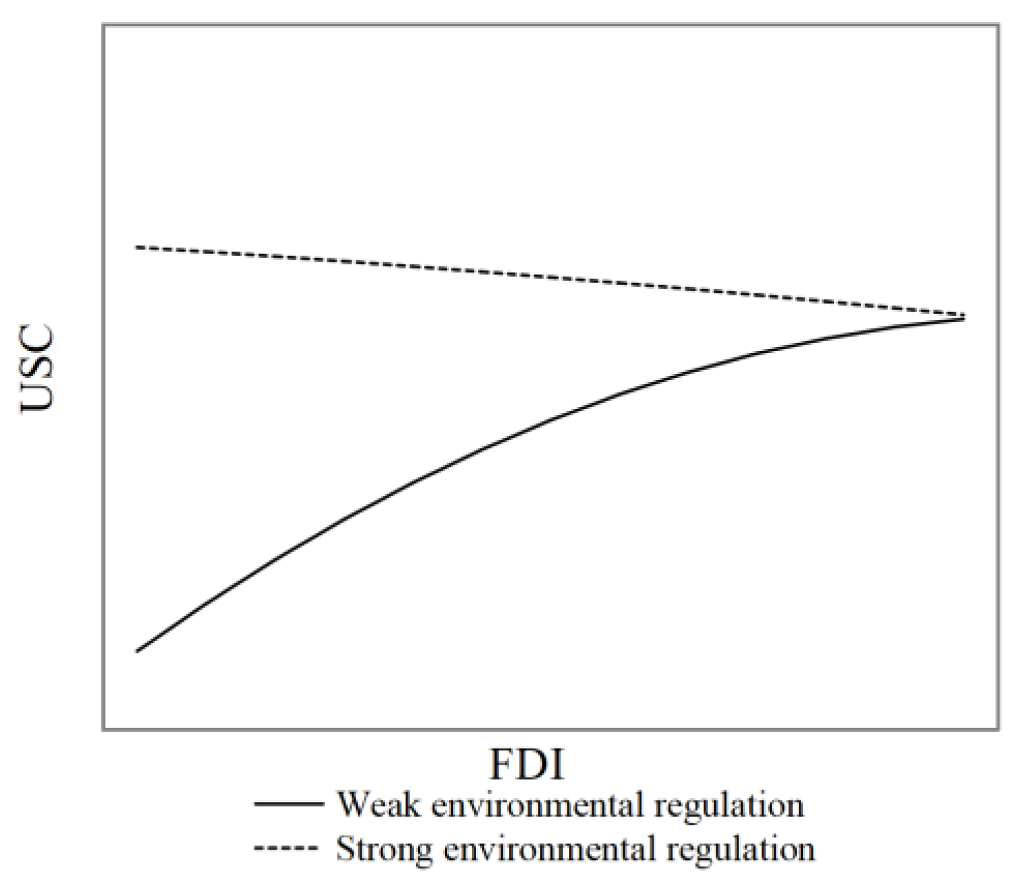
The moderating effect plot in Figure 2 provides a more intuitive picture of the role of environmental regulations. As shown by the dotted line in Figure 2, the impact of FDI on USC is negatively linear under the moderating effect of stringent environmental regulation. In other words, the moderating effect of environmental regulation on FDI is negative: as the size of FDI increases, USC decreases. However, it is evident that when the moderating effect of environmental regulation is weaker, the positive impact of FDI on USC becomes more pronounced, and this beneficial effect is particularly pronounced in cities with lower sustainable competitiveness. The results presented in Figure 2 reveal intriguing insights. Not only do they empirically confirm Hypothesis 2 by affirming the moderating role of environmental regulation in the FDI–USC relationship, but they further uncover heterogeneity in its moderating effects. This implies that regulatory stringency does not always yield optimal outcomes: excessive stringency may prove counterproductive. Moreover, the analysis underscores the necessity of tailoring interventions to local developmental contexts, advocating that policymakers should adopt scientifically informed and contextually appropriate regulatory approaches rather than pursuing uniform maximal stringency.

4.5. Further Discussion: Regional Heterogeneity Analysis

Due to China’s vast territory and large population, regional development differentiation is characteristic, and the introduction of FDI also has obvious regional characteristics. Taking the FDI inflow in 2021 as an example, the proportion of the actual use of foreign capital in the eastern region of China in the total amount of actual use of foreign capital was 84.4%, and the proportions in the central and western regions were 6.2% and 5.3%, respectively. The eastern region already possessed more mature technical conditions and market environment by virtue of its geographical location, policies, and other advantages. Therefore, the differentiation in the amount of FDI in each region may have different effects on sustainable development. To account for geographical disparities, the sample was stratified into four regions: eastern, northeastern, central, and western. Subgroup regression analyses were conducted, and the outcomes are reported in columns (1)–(4) in

Table 8. Regional heterogeneity analysis.

	(1) Eastern Region	(2) Northeastern Region	(3) Central Region	(4) Western Region
fdi	0.439 ***	0.039	−0.126	0.022
	(2.892)	(0.495)	(−1.239)	(0.088)
fdi2	−1.263 ***	−0.108	0.250	0.064
	(−3.212)	(−1.019)	(1.408)	(0.072)
econ	0.000	−0.000	0.000	−0.000
	(1.484)	(−0.282)	(0.496)	(−0.509)
stru	0.000	0.000	0.001	0.001 *
	(0.189)	(0.333)	(0.980)	(1.675)
pop	−0.034	−0.094	−0.072 ***	−0.092 ***
	(−1.138)	(−1.652)	(−3.155)	(−2.652)
inter	0.770 ***	1.087 **	0.867 *	−0.153
	(3.776)	(2.361)	(1.877)	(−0.387)
gov	−0.047 **	0.058 **	0.083 ***	0.065 **
	(−2.273)	(2.712)	(3.369)	(2.492)
trade	−0.001	−0.003	−0.004	−0.002
	(−0.146)	(−0.781)	(−0.900)	(−1.073)
Constant	1.383 ***	0.069	−0.373	−0.092
	(3.860)	(0.175)	(−1.025)	(−0.218)
Individual and time effects	Yes
N	744	264	681	648
Control variables	Yes
R2	0.559	0.627	0.620	0.518

Note: values in parentheses denote t-statistics; ***, **, and * indicate statistical significance at the 1%, 5%, and 10% levels, respectively.

. The comparison shows that the estimation coefficient of fdi is significantly positive only in the eastern region, and the estimation coefficient of fdi² is significantly negative. The impact of FDI on USC in the eastern region is the inverted U shape, but the impact of FDI in the northeastern, central, and western regions is not significant. In terms of control variables, the optimization of industrial structure can effectively improve the USC in the western region, and population size, the number of Internet employees, and the government expenditure all have a significant impact on most regions. The population size in the western region has the most obvious negative effect on USC, the number of Internet employees of the northeastern region has the most obvious positive effect on the USC, and the government expenditure in the central region has the most obvious positive effect on USC, but it can negatively affect the USC in the eastern region.

5. Discussion

Our empirical findings robustly confirm an inverted U-shaped relationship between FDI and urban sustainable competitiveness (USC), as hypothesized. The calculated turning point at an FDI/GDP ratio of 29.06% delineates two distinct phases of FDI’s impact on USC, with critical implications for China’s development trajectory. The first phase was growth-driven enhancement (FDI/GDP < 29.06%). In this phase, FDI inflows significantly boosted USC, aligning with China’s early-stage advantages in labor abundance, resource availability, and market scale. These factors have historically attracted FDI into labor-intensive and export-oriented sectors, driving rapid economic growth and employment [35]. Notably, post-2012 policy shifts toward green FDI—evidenced by a 34% increase in renewable energy sector FDI between 2012 and 2020—amplified positive spillovers through technology transfers in clean production and smart infrastructure [36]. The significantly positive coefficients for economic growth and industrial upgrading further validate this trajectory, as GDP per capita gains enabled fiscal investments in eco-parks and digitalization, while tertiary sector expansion reduced energy intensity in high-FDI cities [37]. The second phase was saturation and degradation (FDI/GDP > 29.06%). Beyond the threshold, FDI’s marginal effect turned negative, reflecting the dominance of pollution haven dynamics. Despite policy efforts, manufacturing FDI—which accounted for more than half of total inflows in 2020—remained concentrated in carbon-intensive subsectors (e.g., chemicals, metals), driving a sharp rise in industrial SO₂ emissions in high-FDI regions [21]. This aligns with the significant negative coefficient for population size, where urban overcrowding in FDI hubs like Shanghai and Guangzhou exacerbated congestion costs and PM2.5 levels, offsetting agglomeration benefits. Especially in recent anti-globalization shocks, such as geopolitical tensions (e.g., U.S.–China trade war) and the COVID-19 pandemic, the inverted U-shaped relationship has been further strained.

Second, we revealed a critical result regarding the moderating role of environmental regulation in the FDI–USC relationship: while stringent environmental regulation weakens the positive impact of FDI on USC, relaxed regulations amplify it, particularly in cities with lower sustainable competitiveness, which underscores the nonlinear and context-dependent nature of environmental regulation’s effectiveness and challenges the assumption that stronger regulation always yields better outcomes. The negative moderating effect of stringent environmental regulation can be attributed to escalating compliance costs and regulatory barriers. Strict environmental standards impose significant financial and operational burdens on foreign firms, particularly those in pollution-intensive sectors. These costs may deter long-term investments or incentivize firms to relocate to regions with laxer regulations, exacerbating the pollution haven effect. For instance, multinational corporations facing stringent environmental regulation in high-compliance cities might prioritize short-term cost-cutting over green innovation, ultimately undermining USC. Furthermore, stringent regulations may stifle technological spillovers by limiting FDI inflows or restricting collaboration between foreign and domestic firms. In contrast, weaker environmental regulation reduces entry barriers to FDI, allowing host cities—especially those with limited institutional capacity—to attract capital, generate employment, and foster industrial upgrading. In weakly competitive cities, relaxed regulations create a pragmatic balance: FDI inflows stimulate economic growth through labor-intensive manufacturing and basic technology transfers, even if these activities initially lag in environmental performance. Over time, such growth can build foundational capacities for future green transitions.

Third, the regional heterogeneity analysis reveals stark disparities in the impact of FDI on USC across China’s eastern, northeastern, central, and western regions, reflecting profound differences in economic structures, institutional capacities, and developmental priorities. In the eastern region, FDI demonstrates a robust positive effect on USC, with a significant inverted U-shaped relationship indicated by a negative quadratic term. This suggests that moderate FDI inflows enhance sustainability through technology spillovers and industrial upgrading, but excessive FDI may trigger diminishing returns due to resource congestion, environmental pressures, or market saturation. As the eastern region absorbs approximately 70% of China’s FDI, its high-density economic zones face unique challenges: while advanced infrastructure and innovation ecosystems attract high-quality FDI, over-reliance on quantity-driven growth risks crowding out domestic innovation and exacerbating pollution. In contrast, the northeastern, central, and western regions exhibit weaker or even negative FDI effects, highlighting systemic barriers to leveraging foreign capital. The northeastern region’s statistically insignificant FDI coefficient likely stems from its legacy industrial structure dominated by state-owned heavy industries, which are less responsive to FDI-driven innovation. Rigid institutional frameworks and outdated production models further constrain technology absorption, leaving FDI unable to catalyze meaningful upgrades. Similarly, the central region’s negative FDI coefficient reflects its reliance on low-value-added manufacturing and limited technological capacity. Foreign firms in these regions often operate in labor-intensive sectors with minimal spillovers, while weak intellectual property protections and underdeveloped R&D ecosystems hinder knowledge transfer. In the western region, despite insignificant FDI effects, the positive coefficient for industrial structure signals nascent potential for FDI to drive structural shifts toward higher-value activities, though this requires targeted interventions to address infrastructure gaps and skill shortages.

6. Conclusions

6.1. Conclusions and Research Limitations

FDI has provided China with new ideas and impetus for exploring ways to enhance USC. Adopting scientific and reasonable environmental regulations to attenuate the negative effects of FDI is crucial to facilitating the benign interaction between FDI and USC. We empirically analyzed the role of FDI on USC and further reveals the moderating role of environmental regulation, using data from 281 cities in China from 2012 to 2020 as a sample. Our analysis draws the following conclusions:

First, we confirm a robust inverted U-shaped relationship between FDI and USC, characterized by initial benefits that diminish and eventually reverse as FDI exceeds region-specific thresholds (FDI/GDP = 29.06%). However, beyond the threshold, the negative marginal effects dominate, driven by resource congestion, environmental degradation, and heightened competition for limited ecological capacity. At the regional level, there is also an obvious threshold effect of FDI in the east, and the impact on USC is negative only when its quantity is larger than the threshold; FDI in the northeastern, central, and western regions is small and has no obvious impact on USC.

Second, environmental regulation can regulate and optimize the effect of FDI on USC. The lax environmental regulation can better exert its positive regulating effect on FDI due to the innovation compensation effect, but stringent environmental regulation can even negatively regulate FDI instead.

While this study provides insights into FDI’s role in urban sustainability, certain limitations warrant acknowledgment. First, although the USC index aggregates six dimensions of knowledge, harmony, ecology, culture, regional integration, and information connectivity, the analysis did not disaggregate these components to explore their individual responses to FDI. Subsequent research could address this gap by compiling granular data for each subdimension, enabling a more nuanced assessment of FDI’s differential effects on specific facets of sustainable development. Second, FDI has quality in addition to quantity; our study only analyzed it from the perspective of quantity, and more interesting conclusions may be obtained if we look at it from the perspective of quality. However, it was difficult for us to find city-level data about the quality of FDI. In the future, we can construct empirical models at the firm level and sustainable development indices to compare and analyze the quantity and quality of FDI at the same time. Third, the dataset may over-represent cities with better data availability, underweighting smaller or less-developed regions. This could have biased the conclusions toward urban contexts with higher institutional capacity. In addition, the findings are context-specific to China, and their applicability to other developing economies (e.g., African nations with weaker governance) or developed countries remains untested.

6.2. Recommendations

To maximize the positive impact of FDI on USC while mitigating its potential risks, policymakers should establish dynamic and differentiated environmental regulation frameworks tailored to regional realities and optimize FDI attraction strategies. First, given the inverted U-shaped relationship between FDI and USC, a threshold-responsive mechanism should be implemented. In high-FDI-intensive regions such as eastern China, dynamic environmental regulation standards should be set based on the real-time monitoring of FDI scale and quality. When FDI exceeds the reasonable threshold, regulatory stringency should be gradually increased, mandating foreign enterprises to adopt clean technologies or participate in ecological compensation projects to curb resource competition and pollution aggravation. In contrast, central and western regions with lower FDI volumes may moderately relax environmental access in the short term but must simultaneously strengthen infrastructure development and green technology training to lay the groundwork for attracting high-quality FDI in the future.

However, the risks of weak environmental regulation should not be overlooked. While it amplifies FDI’s short-term benefits, prolonged regulatory leniency may lock cities into polluting industries, delaying sustainable development. The key lies in recognizing that environmental regulation’s optimal intensity varies with local absorptive capacity and development stage. Policymakers must therefore adopt adaptive, science-driven approaches that align regulatory stringency with local economic thresholds and institutional readiness, rather than pursuing uniform maximalism. This nuanced perspective not only reconciles the dual role of FDI as both an economic catalyst and an environmental risk but also advances the broader goal of harmonizing globalization with sustainability.