Characterization of Energy Profile and Load Flexibility in Regional Water Utilities for Cost Reduction and Sustainable Development

Abstract

Water utilities use a significant amount of electrical energy due to the rising demand for wastewater treatment driven by environmental and economic reasons. The growing demand for energy, rising energy costs, and the drive toward achieving net-zero emissions require a sustainable energy future for the water industry. This can be achieved by integrating onsite renewable energy sources (RESs), energy storage, demand management, and participation in demand response (DR) programs. This paper analyzes the energy profile and load flexibility of water utilities using a data-driven approach to reduce energy costs by leveraging RESs for regional water utilities. It also assesses the potential for DR participation across different types of water utilities, considering peak-load shifting and battery storage installations. Given the increasing frequency of extreme weather events, such as bushfires, heatwaves, droughts, and prolonged cold and wet season floods, regional water industries in Australia serve as a relevant case study of sectors already impacted by these challenges. First, the data characteristics across the water and energy components of regional water industries are analyzed. Next, barriers and challenges in data acquisition and processing in water industries are identified and recommendations are made for improving data coordination (interoperability) to enable the use of a single platform for identifying DR opportunities. Finally, the energy profile and load flexibility of regional water industries are examined to evaluate onsite generation and battery storage options for participating in DR operations. Operational data from four regional sites across two regional Australian water utilities are used in this study.

1. Introduction

1.1. Overview and Motivation

The energy demand for water utilities is rising because of increased water demands in households and industries, higher wastewater treatment needs due to environmental issues, and the growing use of desalination to preserve limited groundwater resources [1]. According to the International Energy Agency (IEA) report, the amount of energy used in the global water sector is projected to double by 2040 [2], as shown in Figure 1. This projection is based on the global energy demand for water supply, distribution, desalination, reuse, large-scale transfer, and wastewater treatment under a business-as-usual scenario. It is seen from the figure that in 2014, the total global energy demand in the water sector was 800 TWh and is expected to exceed 1400 TWh by 2040. While the projection accounts for current trends, it does not fully incorporate the potential impact of future advances in water–energy management or energy-saving technologies, which could mitigate some of the anticipated demand increase. The rising energy demand is leading to higher operational costs and negative environmental effects [3]. Greenhouse gas emissions from the water sector currently account for 2–4% of global emissions and are expected to increase in the coming years [3]. Establishing onsite renewable generations and optimized energy and load management can solve higher energy costs and reduce dependency on grid electricity [4,5].

Urban water utilities typically have limited geographical land area and primarily rely on grid electricity. In contrast, regional water sites often have larger land areas and greater potential to integrate onsite renewable energy sources such as solar PV, wind, and hydro. Additionally, some water utilities can generate electricity using biogas, a byproduct of their operations. DR participation using available load flexibility can reduce their operating cost and support the grid by providing ancillary services [6,7]. Therefore, regional water utilities have more opportunities to engage in various DR mechanisms. However, limited research has been conducted in DR for water utilities and even less for those in regional areas.

1.2. Literature Review

Energy use in the water industry varies greatly, from 5% to more than 40% of operational costs [4,8]. Within the water industry, three factors mainly influence energy usage. The first factor is the type of facility, whether it is a pumping station, wastewater treatment plant, or desalination plant. Overall, pumping stations have the lowest energy consumption, followed by wastewater treatment facilities, with desalination being the most energy-intensive. Wastewater goes through three types of treatment [9]. The primary treatment is a major treatment that separates solids from the liquid and removes grease. The secondary treatment uses a biological process to remove most biological oxygen demand and influent suspended solids. The tertiary treatment removes nutrients (such as phosphorous and nitrogen) and most effluents and suspended solids. Tertiary treatment requires twice the energy of secondary treatment, which itself consumes twice the energy of primary treatment. However, not all wastewater treatment plants implement all three stages, leading to variations in energy consumption depending on the level of treatment before discharge.

The second factor affecting energy consumption is the method of water retrieval and discharge, i.e., whether it is gravity-fed or pumped against gravity, with the latter being more energy-intensive. For instance, the cost of pumping water in Adelaide and Sydney is higher than in Melbourne due to differences in water catchment systems. Melbourne benefits from gravity-fed supplies sourced from mountain catchment storages, whereas Adelaide and Sydney rely on energy-intensive pumping from rivers [9,10,11]. The use of desalination pumps and the optimal scheduling of water supply significantly affects the energy consumption of the water sector [12,13,14].

The last factor affecting the energy use of the water industry is the type of users and their geographical locations. In Australia, household users consume 12% of water, but the cost of servicing them contributes to 51% of total Australian water industry costs [15]. The higher costs are due to the higher-quality water demand of household users. Regional users’ challenges are even greater than those of urban users as they face higher costs and lower reliability, and users in remote communities have lower-quality water services, such as the lack of wastewater treatment [15]. Despite the challenges faced by regional water industries, there is a lack of research on regional water industries [15].

Climate change presents another significant challenge to the water industry. As the climate becomes hotter and drier, desalination becomes a necessity. As of 2015, there were 17,000 desalination plants in over 150 countries, with only 1% of their energy coming from renewable sources [16]. Desalination is an energy-intensive process, and if all new water sources in Australia’s major cities come from desalination, it is estimated that energy demand will increase three to fourfold [9].

In major Australian cities, 76% of energy demand from water utilities is met by traditional energy sources [9], so implementing energy-saving measures will also reduce greenhouse gas emissions. Existing energy-saving methods include using more efficient processing techniques, onsite renewable energy generation, pump scheduling, energy efficiency optimization [17,18,19,20], and, more recently, demand response energy management [4,21].

A study of 25 European sites in [18] showed that energy cost savings of 5% to 35% are possible. A more recent study in India shows that energy consumption can be reduced by 35% after implementing high-efficiency pumps at small Water Treatment Pumps (WTPs) [22]. The implementation of high-efficiency pumps and AI-based optimization can reduce the energy consumption at WTPs by 20–30% [23]. Melbourne Water aimed to save AUD 3.5 million annually in energy costs by using renewable energy [24]. Onsite energy generation can come from embedded energy, which includes resources collected or produced by water industries, such as biogas and hydro. In 2018, the Australian water industry generated 18% of its energy onsite from renewable sources [25]. Biogas and hydro were the main sources of onsite energy generation, but they may have reached their full capacity: 80% of biogas capacity by 2002 and 95% of hydropower by 2010 [26]. Since around 2013, the adoption of solar PV has accelerated as the technology has become more mature and economically viable [26]. Wind power has been proposed for water industries but has not been widely adopted due to its impact on local communities, including noise, aesthetics [26], limited productive period, land area, and resource constraints [27]. However, some success has been reported, with cost savings of 16% [28].

While renewable energy holds great potential for reducing the carbon footprint of water and wastewater treatment systems, its practical implementation faces several challenges. For example, the inherent uncertainty and intermittency of solar PV and wind generation pose significant concerns, particularly for processes in the water sector that demand a continuous and stable power supply [29]. Without adequate mitigation—such as optimal system design, energy storage solutions, or hybrid systems incorporating backup sources or grid connectivity—these fluctuations can lead to operational disruptions. A case study of the water–electricity nexus in China provides a roadmap toward sustainable energy and electricity by integrating a mix of electricity generation and storage systems [30]. Similarly, a case study from Karpathos, Greece, demonstrated the successful implementation of a hybrid system combining solar PV, wind turbines, and energy storage, effectively addressing the variable nature of renewable energy resources [31]. Additionally, the deployment of such technologies often requires substantial land area and is subject to complex regulatory approval processes, which can further hinder implementation. Facilities utilizing biogas for energy generation faced challenges in maintaining biogas production levels due to seasonal variations in organic waste content. Moreover, while biogas systems contribute to energy self-sufficiency, their scalability and maintenance costs remain significant barriers [32].

Demand response (DR) is a more recent energy-saving initiative [21,33,34], where water utilities voluntarily adjust their energy use in response to electricity pricing that varies seasonally, hourly, or half-hourly. Energy savings can be achieved by scheduling pumps [35] and optimizing tank design [28] or by taking it a step further to forecast electricity prices [36]. While the concept is simple, it is difficult to generalize due to the water industry’s risk aversion, the lack of studies on its benefits, the complexity of price changes, access to price offers, and the need to accurately predict energy usage.

Several studies in the water sector focus on urban areas [37,38]. Linkage analysis has been used in [37] to identify the mutual influences of water and energy consumption and interactions among different economic sectors in Beijing. In a similar study [38], the interconnections between energy consumption and water use in a city were analyzed using a system-based framework. A recent study [25] investigated the amount of renewable energy generation by the Australian water industry from different sources such as biogas, solar PV, and hydropower. In 2018, the amount of on-site renewable energy generated by the Australian water industry was 279 GWh/y, which was 18% of the total energy demand of the water industry. Solar PV contributed only 1% (2.2 GWH/y) of this total amount due to the lack of space requirement for larger systems. However, regional or remote areas offer opportunities that their urban counterparts lack: space to install large electricity generation systems [20]. For example, the world’s largest solar farm will be built in a remote area in the Northern Territory, Australia [39].

Therefore, this paper focuses on water industry data analysis and energy mapping to identify opportunities and reduce electricity costs. The use of on-site renewable generation such as solar PV and storage installation is expected to increase economic benefits and enhance the sustainable development of the water–energy nexus.

1.3. Contribution

In this paper, the energy profiling and load flexibility of regional water utilities are characterized to analyze the potential DR participation, integration of RESs, and battery storage for cost reduction and sustainable development in the water industry. Several studies have been conducted so far to analyze energy consumption in urban water industries [4,37,38,40,41,42,43]. However, there is a noticeable gap in the literature focusing specifically on regional water utilities, particularly those located in diverse geographical settings with varying energy consumption profiles. This study is unique in that it identifies the barriers to energy profiling and explores the potential for DR and onsite renewable energy integration in WTPs and pumping stations, with a focus on sustainable development and electricity cost reduction in regional areas.

The diverse nature of water industries, vast land area, and exposure to extreme weather conditions make regional Australia an ideal candidate for this study. Four regional Victorian water utility sites with a mix of WTPs and pumping stations were considered in this study, which had different characteristics: site A serviced domestic and water-intensive industry users in areas with higher annual rainfall, while site B serviced domestic and smaller industries. Therefore, they offered a more direct comparison of the impact of cost or energy savings in water industries with different demands and operating environments. Other key features of this study are listed below.

• Step-by-step data analytics was developed to discover, interpret, and visualize meaningful patterns from water industry energy consumption data. The developed method helped deliver a clean energy profile to characterize and identify energy flexibility for water utilities, especially in regional areas.
• The identified energy flexibility was used to explore the opportunities for cost reduction in the operation of water utilities through demand management. Several levels of demand management were considered to identify the quarterly and yearly savings of a water utility.
• The opportunities and benefits of installing solar and battery storage in the regional water industry sites were assessed for cost reduction and sustainable development.
• Recommendations are made for improving data coordination (interoperability) to enable the use of a single platform for identifying DR opportunities for different types of water utilities.

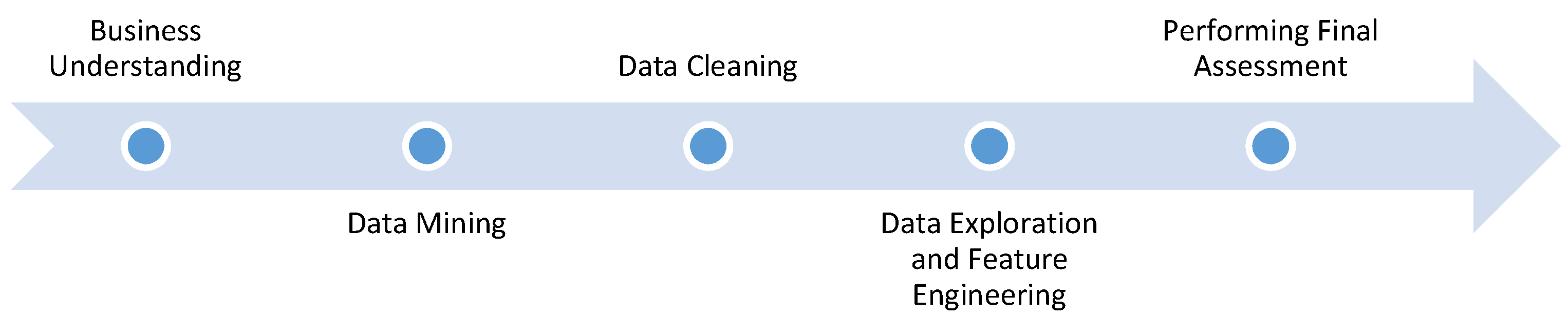
Data from four regional sites of two Australian water utilities were collected and analyzed. Among these four sites, two were water treatment plants and two were water pumping stations. The pumping stations mostly pumped water to upstream reservoirs, while the water treatment plants had distinct processes for treating wastewater. Electricity from the grid was the main energy source of these participating water utilities, but other energy sources such as hydro, biogas, solar, and diesel were also used as secondary energy supplies.

The rest of this paper is organized as follows: Section 2 describes the data analysis methodology and performance parameters used in this study. Section 3 presents and explains the energy profiling and results. Finally, Section 4 provides conclusions and discusses future work.

2. Methodology

Data analytics were performed to discover, interpret, and visualize meaningful patterns from the data provided by different water utilities. Generally, the data analysis process included examining past data through collection, inspection, modeling, and questioning. In this study, a series of well-defined data analytical steps were followed to map water and energy data and assess DR opportunities in the water industry. These steps are presented in Figure 2 and briefly described below.

• Step 1: Business Understanding

In this step, relevant questions were identified through project meetings and correspondence to understand the operations of water utilities and the description of the provided data, which enabled the researchers to achieve the project goals.

• Step 2: Data Mining

Necessary and relevant data were requested and gathered from water utilities. However, unavailable data needed to be prepared using information and observation of the system characteristics and data relationships. Necessary unavailable data such as weather data could be collected from third-party providers like the National Renewable Energy Laboratory (NREL).

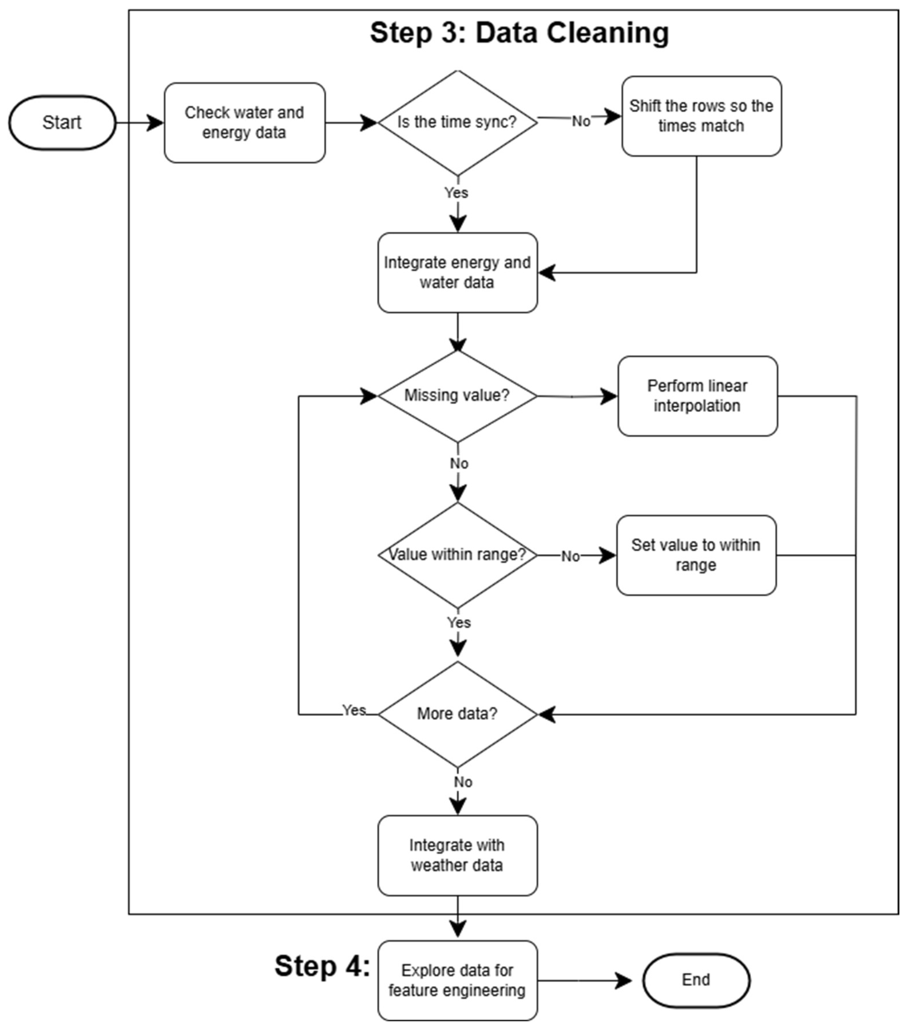
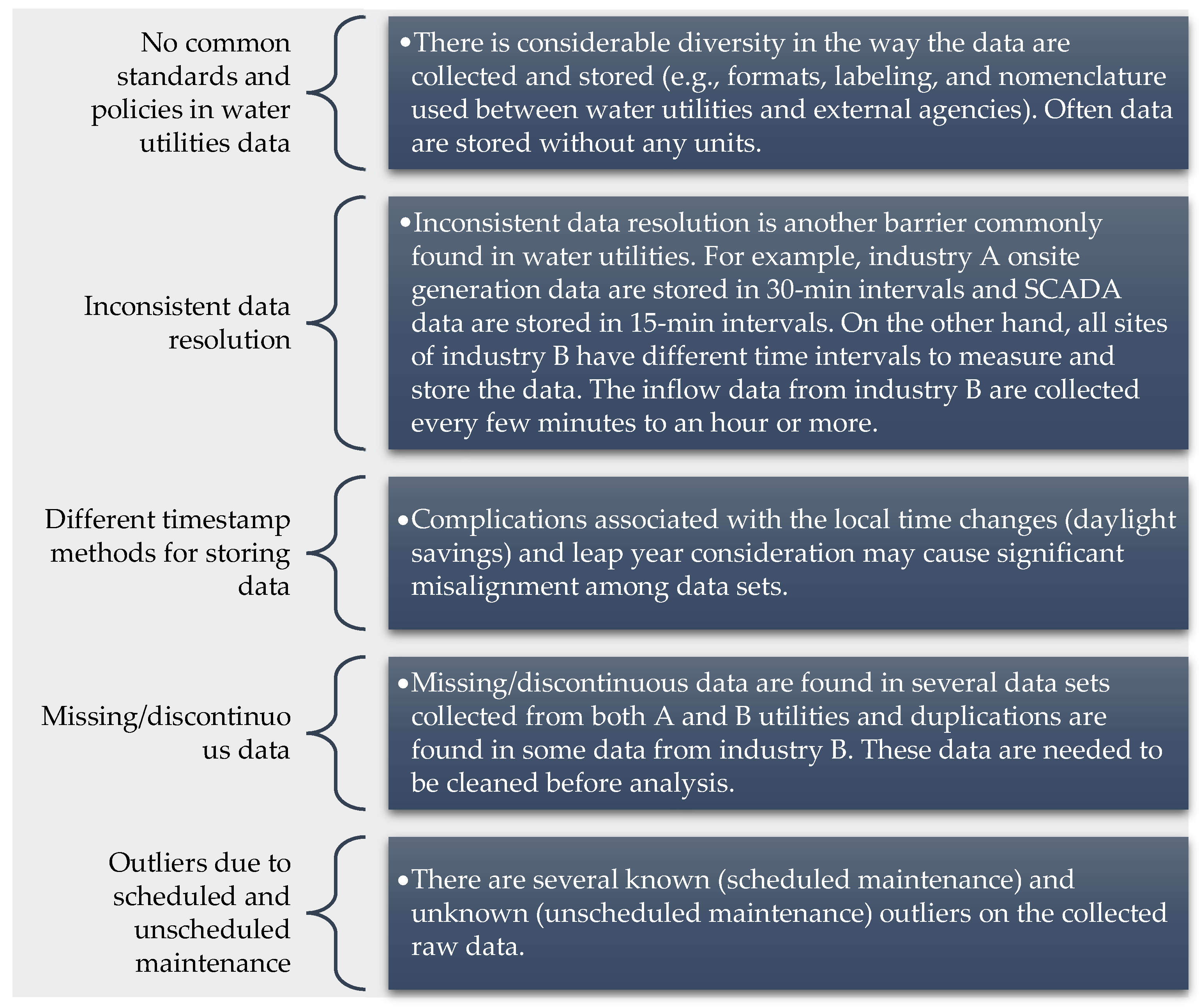
• Step 3: Data Cleaning

To achieve higher accuracy in analytical results, inconsistent data were cleaned and missing data were generated using the linear interpolation method. Data were collected from various sensors and different systems, so errors could occur due to various reasons, including hardware failures or other environmental factors. To achieve higher accuracy in the analytical results, data were pre-processed. The following errors were observed:

• Values beyond reasonable operational limits, possibly due to hardware errors.
• Missing values, possibly due to hardware errors or data collection at different time scales. For example, energy consumption was collected half-hourly, but some water pumps were collected hourly or nearly hourly.
• Time was not synchronized. The timing of the data could be out of synchronization because they were collected from different sources. To overcome this issue, we matched the events to energy consumption.

The data cleaning process for each error type and how it related to the next step of data analytics (Step 4) is illustrated in the flowchart in Figure 3.

• Step 4: Data Exploration and Feature Engineering

Hypotheses about the defined objectives were formed by visually analyzing the data. More meaningful features could be constructed by selecting important features from the available raw data. For example, a water factory had two types of water inflows: raw and controlled. After investigating the data, we found that the controlled flow was more meaningful as it coincided with energy consumption.

• Step 5: Performing a Final Assessment

The cleaned and processed data were utilized to perform the necessary analysis on DR participation and the potential for RES and battery storage installation to reduce electrical energy costs.

2.1. Data Classification and Diversity

Water utilities collect various types of data depending on their categories and working principles. For example, pumping stations might have only inflow and outflow information, while water treatment plants would have additional parameters such as energy used, water temperature, suspended solids (SSs), biological oxygen demand (BOD), chemical oxygen demand (COD), NH4 flow, etc. [41,44]. However, only some of these parameters are useful for mapping the characteristics of the data across water and energy components. Useful parameters include historical electricity/energy generation and consumption data, water inflow and/or outflow data, and weather data.

The electricity generation data sources could be centralized Supervisory Control and Data Acquisition (SCADA) systems or distributed single or multiple NMIs at different locations. The energy data were represented as import or export electricity based on the convention used at each specific plant. There is also a lack of standardization among water utilities in how they format and store data. Consequently, it is challenging to achieve the interoperability of data among water utilities to achieve common goals such as load aggregation to participate in wholesale DR. For example, some meters measure voltage or currents instead of power or energy consumption. To address this issue, relevant equations can be applied based on the device’s rating to derive the energy data.

For data related to the water inflow and outflow, different parameters used in water treatment processes are useful in identifying the relationship between energy consumption and related water treatment processes, and many researchers use these parameters for forecasting energy consumption [41,44,45,46,47,48,49]. Identifying the relationship between energy and water data will help map load flexibility in participating DR utilities.

Since electricity demand, pricing, water pumping, and treatment are highly or moderately dependent on weather conditions, reliable weather data are essential for accurate mapping and ensuring load flexibility. Weather data can be collected from onsite weather stations or reliable third-party providers such as Scientific Information for Land Owners (SILO) [50] and NREL [51].

Several initiatives have been undertaken globally to establish standards and common frameworks for water utility data sharing. For instance, the water data transfer format (WDTF) developed by the Bureau of Meteorology (BoM) standardizes how Australian water agencies submit water data to the BoM [52]. Additionally, Smart Cities—FIWARE is an open-source platform used in smart cities across Europe that facilitates data interoperability across the water, energy, transport, and waste sectors [53]. However, there remains a significant gap in dedicated standards and frameworks specifically designed for water utility that includes integrated data types such as water inflow/outflow, water levels, energy consumption and generation, and weather data such as rainfall, irradiance, etc.

2.2. Data Cleaning and Preparation

In general, data can be missing due to communication, meter, or collection failures. For water utilities, much of the data are collected using sensors, which can be erroneous due to failures or limitations within minimum and maximum boundaries. Some sensors only initiate and take measurements under specific conditions, resulting in the absence of continuous time series data. In such cases, interpolation using system information and relevant system behaviors is performed to synthesize the missing values.

Some data points, such as time series energy generation from backup diesel generators, are not stored. Limited information is found from logbooks, such as how many hours or days the generator operated. If any data are completely unavailable, then data can be synthesized using equations.

2.3. Wholesale and Retail Energy Tariff

Understanding electricity prices or tariffs and their changing patterns is important for performing DR analysis. Electricity prices in the deregulated energy market vary with time, mainly governed by the available supply and demand for electricity. In general, there are two types of electricity pricing: wholesale and retail pricing [54]. Retail prices are fixed for customers and broadly divided into peak and off-peak prices. On the other hand, wholesale or spot prices fluctuate depending on the real-time variations in the present and historical supply and demand of electricity [55]. Examples of wholesale and retail tariffs are presented in Figure 4. In Figure 4a, the variation in the Australian NEM electricity spot price in Victoria from 23–29 July 2018 is presented. Since 2018, energy consumption data have been used for all water utilities, so the corresponding wholesale and retail electricity prices from the same year were also considered in this study. The spot price varies based on the supply and demand of the energy market, changing at a certain time interval, such as 5 or 30 min.

In the heatmap, the color intensity ranges from blue to red, with blue indicating lower prices and red indicating higher prices. Spot prices are low during weekends because of the lower demand for electricity. According to Figure 4a, during weekdays, higher wholesale electricity prices occur from 7 a.m. to 9 a.m. and again from 6 p.m. to 8 p.m. Conversely, lower electricity prices occur from 12 a.m to 6 a.m.

Furthermore, the retail electricity price of an industry is presented in Figure 4b. Peak hours started from 7 a.m. to 11 p.m. from Monday to Friday. The rest of the hours of working days and weekends (Saturday and Sunday) are off-peak hours. Electricity prices are higher during peak hours and lower during off-peak hours. Typically, large industries purchase electricity at fixed rates for peak and off-peak hours throughout the year. From Figure 4a, the highest wholesale electricity price was 159.4 AUD/MWh and the lowest value was 7.94 AUD/MWh. However, the highest and lowest wholesale prices varied throughout the year. From Figure 4b, the peak retail price was 155 AUD/MWh and the off-peak retail price was 110.5 AUD/MWh.

Water utilities that purchase electricity at wholesale prices have significant potential to reduce their electricity bills by managing their loads according to spot price variations, with possible savings of up to 22% [4]. Most water utilities in Australia use retail prices for their electricity consumption. However, some utilities are large enough to participate in wholesale pricing, and others may be eligible to join the wholesale market by partnering with other industries or aggregators. In this work, analyses were performed using both retail and wholesale market prices.

2.4. Performance Index

Several performance indicators are used in the energy sectors to explore the economic operation of a utility. A simple energy efficiency index (EEI) can be defined as the ratio of the volume-weighted average price (VWAP) of electricity and the time-weighted average price (TWAP) of electricity, which can be presented as follows [4]:

$$\mathrm{E}\mathrm{E}\mathrm{I}={\displaystyle \frac{\mathrm{V}\mathrm{W}\mathrm{A}\mathrm{P}}{\mathrm{T}\mathrm{W}\mathrm{A}\mathrm{P}}}.$$

(1)

where EEI is the energy efficiency index, VWAP is the volume-weighted average price of electricity in AUD/MWh, and TWAP is the time-weighted average price of electricity in AUD/MWh.

VWAP can be calculated by using the following steps: First, multiply each 5 or 30 min interval of energy consumption in MWh by its spot price and sum this amount for a specific time such as 3 months, 6 months, or a year. Then, divide this total amount by the total energy consumption in MWh for the specific time. VWAP can be represented as

$$\mathrm{V}\mathrm{W}\mathrm{A}\mathrm{P}={\displaystyle \frac{{\sum }_{\mathrm{T}\mathrm{i}\mathrm{m}\mathrm{e}\mathrm{P}\mathrm{e}\mathrm{r}\mathrm{i}\mathrm{o}\mathrm{d}}{(\mathrm{M}\mathrm{W}\mathrm{h}\mathrm{c}\mathrm{o}\mathrm{n}\mathrm{s}\mathrm{u}\mathrm{m}\mathrm{p}\mathrm{t}\mathrm{i}\mathrm{o}\mathrm{n}\times \mathrm{S}\mathrm{P})}_{5-\mathrm{o}\mathrm{r}30-\mathrm{m}\mathrm{i}\mathrm{n}\mathrm{i}\mathrm{n}\mathrm{t}\mathrm{e}\mathrm{r}\mathrm{v}\mathrm{a}\mathrm{l}}}{{\sum }_{\mathrm{T}\mathrm{i}\mathrm{m}\mathrm{e}\mathrm{P}\mathrm{e}\mathrm{r}\mathrm{i}\mathrm{o}\mathrm{d}}({\mathrm{M}\mathrm{W}\mathrm{h}\mathrm{c}\mathrm{o}\mathrm{n}\mathrm{s}\mathrm{u}\mathrm{m}\mathrm{p}\mathrm{t}\mathrm{i}\mathrm{o}\mathrm{n})}_{5-\mathrm{o}\mathrm{r}30-\mathrm{m}\mathrm{i}\mathrm{n}\mathrm{i}\mathrm{n}\mathrm{t}\mathrm{e}\mathrm{r}\mathrm{v}\mathrm{a}\mathrm{l}}}}.$$

(2)

where SP is the spot price of each 5 or 30 min interval of time.

TWAP reflects the average 30 or 5 min interval spot price of the market and can be calculated by obtaining the average price over a specified time. TWAP can be represented as

$$\mathrm{T}\mathrm{W}\mathrm{A}\mathrm{P}={\displaystyle \frac{{\sum }_{\mathrm{T}\mathrm{i}\mathrm{m}\mathrm{e}\mathrm{P}\mathrm{e}\mathrm{r}\mathrm{i}\mathrm{o}\mathrm{d}}{\left(\mathrm{S}\mathrm{P}\right)}_{5-\mathrm{o}\mathrm{r}30-\mathrm{m}\mathrm{i}\mathrm{n}\mathrm{i}\mathrm{n}\mathrm{t}\mathrm{e}\mathrm{r}\mathrm{v}\mathrm{a}\mathrm{l}}}{\mathrm{N}\mathrm{u}\mathrm{m}\mathrm{b}\mathrm{e}\mathrm{r}\mathrm{o}\mathrm{f}\mathrm{i}\mathrm{n}\mathrm{t}\mathrm{e}\mathrm{r}\mathrm{v}\mathrm{a}\mathrm{l}\mathrm{s}}}.$$

(3)

where SP is the wholesale price of each 5 or 30 min interval of time.

The energy efficiency index (EEI) reflects whether an individual site is operating economically over a specific period, such as quarterly or annually. By evaluating the EEI, water utilities can assess the economic performance of their facilities and identify opportunities for improvement. This may include implementing DR strategies, integrating on-site energy storage, or shifting energy consumption from peak to off-peak hours using renewable energy sources.

According to Equation (1), the EEI value can be greater than 1, equal to 1, or less than 1. An EEI value greater than 1 indicates that the facility is incurring higher operational costs, often due to elevated energy consumption during peak electricity pricing periods. In contrast, an EEI value of less than 1 suggests a more cost-effective operation, where energy use is optimized to avoid peak-hour tariffs. In this study, four Victorian water sites were considered to calculate their EEIs and their savings after implementing DR to optimize the energy demand during peak hours.

One of the focal points of this research was to visually represent water utility data to understand current electricity consumption patterns and explore the opportunities to reduce electricity costs by implementing various demand management strategies for the present load profile.

2.5. Opportunity Assessment Process

The total electricity cost can be reduced by managing loads to operate mostly during off-peak times when the electricity price is relatively low. Financial incentives are also provided to customers for shifting their loads from peak hours to off-peak hours [56]. Another way to manage loads is by using forecasting techniques with historical data, allowing load shifting based on the forecasts [57]. However, the flexibility of shifting loads based on forecasting techniques is limited and, sometimes, water utilities are forced to operate their loads during peak hours. Additionally, retail prices are very high for large customers, making wholesale pricing an attractive option to lower their electricity costs. Customers in wholesale pricing can choose demand management strategies to lower their electricity costs [58]. An overview of the methodology followed for data analyses and DR opportunity assessment is presented in Figure 5.

Another method of reducing operating costs is to use a PV system to supply electricity during the daytime. However, peak times usually occur in the morning and evening when the sunlight is not at its maximum. Therefore, a battery storage system is proposed to store excess solar energy instead of exporting it to the grid. Savings are calculated for different sizes of solar PV systems.

3. Results

This study examined four regional sites from two water utilities located in southeastern and southwestern Australia for energy profiling and load characterization. These utilities are referred to as A and B, with their respective sites labeled as A1, B1, B2, and B3. Among them, A1 and B1 were water treatment plants operated by utilities A and B, respectively, while B2 and B3 were water pumping stations managed by utility B. Outcomes related to data acquisition, processing, and opportunity assessment are discussed in this section.

3.1. Data Acquisition

Energy export and import data from SCADA and NMIs were collected from both water utilities. Water-related data such as in/out flow, flow rate, and water levels were available from all sites. Since B1 was a Sequencing Batch Reactor (SBR) process-based water treatment plant, additional data such as SBR tank water level, water pH level, and dissolved oxygen (DO) level were also available. Weather data were collected from both the SILO website and NREL weather databases, considering the geographical locations of all sites. The weather data included hourly temperature, humidity, evaporation rate, pressure, and daily rainfall.

The barriers and challenges observed during the data acquisition and processing phase are presented in Figure 6.

3.1.1. Data Selection and Processing

Numerous data points from utilities A and B from year 2015 to 2020 were collected. However, there were gaps or incomplete data up until 2018, with complete datasets for utility A available from April 2018 onward. For utility B, most required data were available from 2018 onward.

In 2019, severe bushfires and droughts occurred in eastern Victoria, Australia. Furthermore, COVID-19 impacted the routine lives of people in 2020, with people working from home, dealing with lockdowns, and many other unusual changes in day-to-day life. Therefore, 2018 was considered a more representative year of the normal operational pattern for these water utilities. In other words, using data from 2018 helped avoid significant outliers and unusual pattern changes in the dataset. Most of utility A’s data were available from April 2018 onward. Therefore, April 2018 to March 2019 was considered a one-year study period for A, whereas January 2018 to December 2018 was considered the study year for B.

Weather greatly influences the water usage of individuals and different industries. Initially, weather data were collected from SILO from water utility sites. However, SILO data contain only the maximum and minimum weather data for a day. Therefore, weather data were also collected from NREL, which provides half-hour resolution data. The SILO and NREL weather data were compared and found to be consistent for this project.

Due to the challenges related to the raw data described above, Python scripts were developed to clean, infill, and extract necessary information from raw data files. DR flexibility depends on the electricity price variation at that time. In Australia, the electricity market price varies every 30 min. Therefore, a 30 min data frequency was selected for this project’s data processing and analysis. Electrical energy data, water inflow and/or outflow data, and weather data were collected/converted into 30 min intervals. Linear interpolation was applied to convert different timestamped data into 30 min intervals. Similar methods were used to fill in missing data. Mismatches in the time series data alignment were resolved by considering actual AEST time in Melbourne as the default time rather than daylight savings time. Further time misalignment among different datasets was adjusted by shifting time-series data based on system characteristics and demand–supply relationships. Spurious data were cleaned by removing outliers and utilizing system characteristics and knowledge.

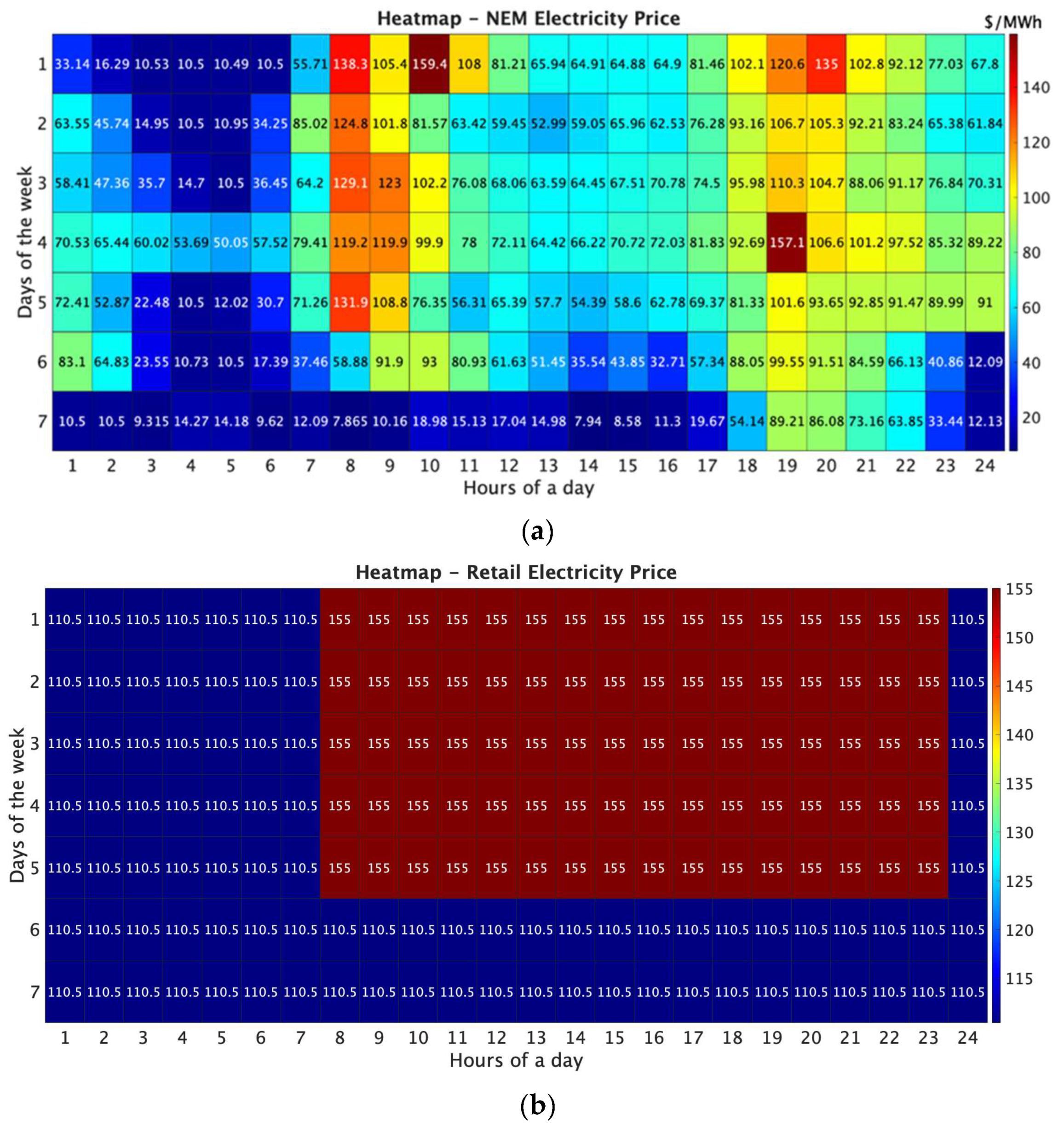
3.1.2. NEM Electricity Spot Price

Understanding historical wholesale prices is necessary to explore the DR opportunities in a water utility. Since energy consumption data from 2018 were used for all water utilities, the corresponding wholesale and retail electricity prices from the same year were also considered. For this project, the data with 30 min interval wholesale electricity prices (AUD/MWh) in Victoria from April 2018 to March 2019 were collected from the Australian Energy Market Operator (AEMO) [55]. An example of hourly energy price fluctuations in the NEM electricity tariff is presented in a heatmap in Figure 4a. The figure shows that higher electricity prices occur from 7 a.m. to 9 a.m. and again from 6 p.m. to 8 p.m. Conversely, lower electricity prices occur from 12 a.m. to 6 a.m. Based on the NEM electricity tariff profile, it is more economical for users to consume less electricity during peak hours (7 a.m. to 9 a.m. and 6 p.m. to 8 p.m.) and shift loads to off-peak hours (12 a.m. to 6 a.m.).

3.2. Energy Profiling

An energy profile or load profile represents the variations of available generation and loads of a plant. The total load of a site is calculated by adding all available generations or loads at that site. The load or generation data were collected from the SCADA system and NMIs located at different locations. Time series energy consumption for all four sites is presented in Figure 7. From Figure 7, it is evident that energy consumption varies more frequently in water treatment plants because of the turning on and off of different processes during treatment. On the other hand, energy consumption at pumping stations fluctuates less over short periods but indicates seasonal energy variations. For example, energy consumption is higher during hot months, but lower during winter and wet months. Once the energy profile is established, it becomes more feasible to identify load patterns and load flexibility.

During the selected study period, one of the onsite generators at A1 was under maintenance for approximately four months. During this time, a diesel generator was operated for about 9–10 days to participate in DR. The power generation data during this period was unavailable, so it was computed using linear interpolation and system knowledge.

At the B2 and B3 sites, which mainly supplied water to reservoirs, energy consumption was relatively steady throughout their operations. Some steps in the energy consumption profile were visible where pumps of different sizes were brought online to meet varying operational requirements.

On the other hand, B1 was a water reclamation plant that utilized two SBRs for treating wastewater. The SBR process followed specific sequences such as fill, anoxic mix, aeration, and settle, which frequently turned different pumps on and off. These on-and-off sequences caused fluctuations in the B1 energy data.

Once energy consumption and generation profiles are recognized, energy management strategies can be implemented to reduce energy consumption costs.

3.3. Opportunity Assessment

Two methods used in this study for opportunity assessment analysis were ‘peak load shifting’ and ‘battery storage device with PV generation’. Since no participant utility had a solar farm operating in 2018 and 2019, two cases were considered: the base case (without solar) and the with-solar case. In the base case, existing electrical sources such as electricity from the grid, biogas, hydro, and diesel were considered. The solar case included a hypothetical PV generation scenario for the participating utilities. Time series solar generation data were simulated utilizing site locations and their corresponding PV generation specifications. System modeling and PV generation data were obtained from the techno-economic software SAM developed by NREL. SAM is widely used for decision-making by professionals in renewable industries ranging from project managers to engineers, developers, and researchers.

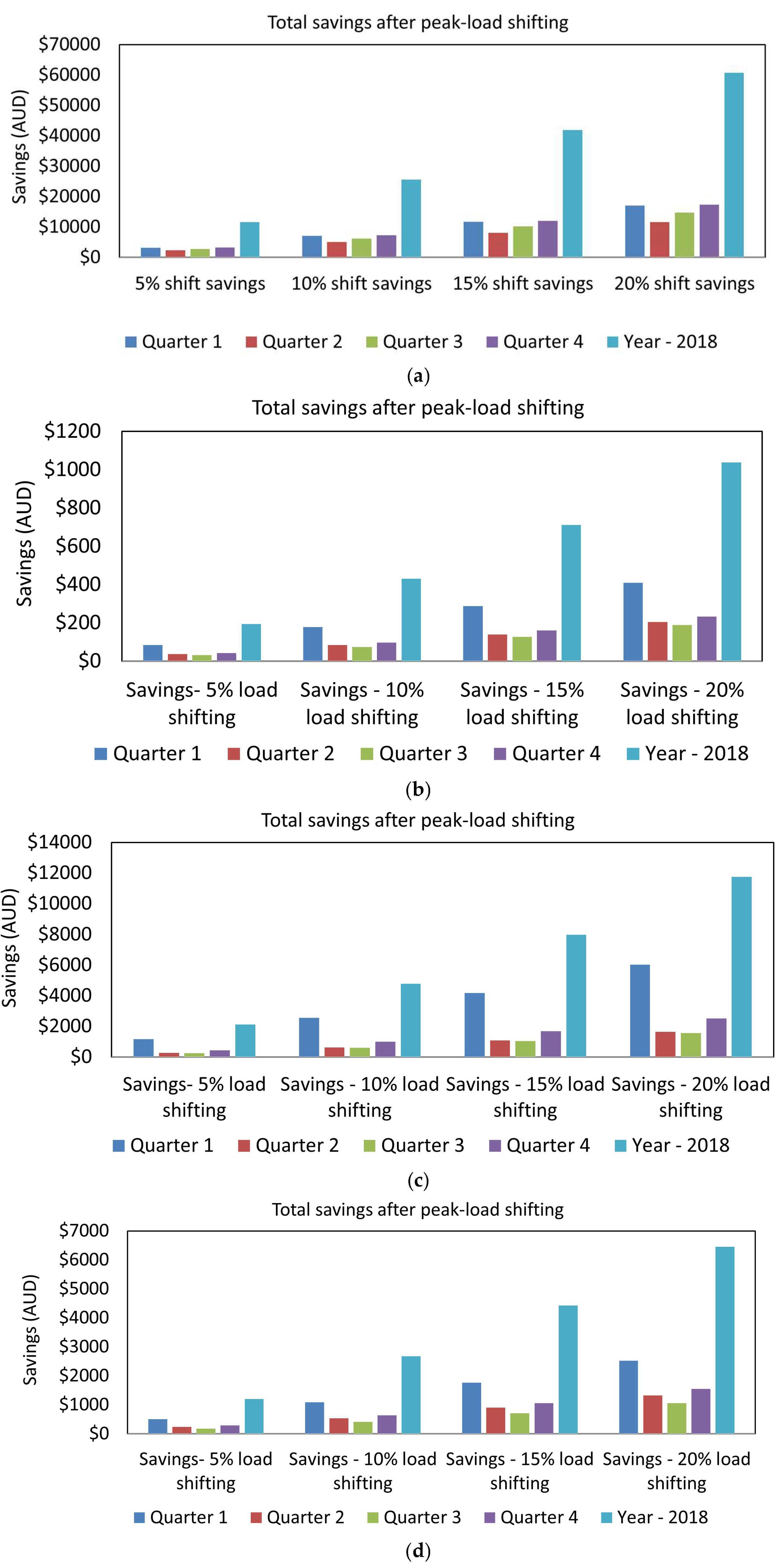
3.3.1. DR Using Peak Load Shifting

All participating sites used retail pricing for billing. For this reason, DR analysis was performed using the retail price. However, there is potential for water industries to participate in wholesale demand response as an individual provider or by joining an aggregator. Similar demand management analyses were performed using the wholesale market price. In retail pricing, the peak hours are from 7 a.m. to 11 p.m. on weekdays, while the rest of the hours are off-peak. The historical spot pricing heatmap used in this paper shows that higher wholesale electricity prices occur from 7 a.m. to 9 a.m. and again from 6 p.m. to 8 p.m. Conversely, lower electricity prices occur from 12 a.m. to 6 a.m., as shown in Figure 4a. Therefore, in wholesale pricing, 7 a.m. to 9 a.m. and 6 p.m. to 8 p.m. are considered peak hours and 12 a.m. to 6 a.m. are considered off-peak hours.

For EEI and savings calculations, different percentages (5%, 10%, 15%, and 20%) of loads from peak hours were shifted to off-peak hours. The percentages considered in this analysis were intended to illustrate the impact of DR on the system’s economic performance and potential savings on electricity bills. However, the actual percentage of load shifting is highly dependent on several factors such as plant type, service requirements, and the degree of operational flexibility. For instance, plants A1 and B1 considered in this study were water treatment plants with several pumps to serve various stages of the water treatment process. Some of the pumps were not critical for maintaining core processes. These loads could be shifted from peak hours to off-peak hours. Pumps involved in critical operations lack such flexibility. On the other hand, B2 and B3 were pumping stations that supplied upstream service areas. If the demand in these areas is relatively low and supported by large reservoirs, greater flexibility for DR can be achieved. However, during emergency situations such as firefighting events, participation in DR becomes infeasible due to the inflexible nature of the load requirements.

The EEI values were calculated using the retail and wholesale prices received from all sites (see

Table 1. Original EEIs for different periods in 2018.

Sites/ Period	EEI (Using Retail Price)				EEI (Using Wholesale Price)
	A1	B1	B2	B3	A1	B1	B2	B3
Q1	1.004	0.994	1.001	0.999	0.983	1.051	0.998	1.002
Q2	0.995	0.997	0.999	0.999	1.005	1.002	0.958	0.988
Q3	0.998	0.999	1.002	0.997	1.005	0.996	0.984	1.016
Q4	1.002	0.995	1.001	0.996	1.004	1.003	0.990	1.006
Annual	0.990	1.002	1.038	1.003	0.995	1.021	1.016	1.008

). EEI values greater than 1 indicated that these sites were not operating economically during those periods. Several EEI values using wholesale prices were higher than those using the retail price, as depicted in Table 1. This is because the wholesale price fluctuates and sometimes rises significantly during seasonal peak hours. Wholesale demand response participants typically follow price forecasts and seek alternatives during peak hours instead of purchasing electricity from the wholesale demand response market, avoiding higher operating costs.

Next, we investigated the impact of load shifting, i.e., shifting loads from peak to off-peak hours, to reduce energy costs in two pricing scenarios: retail and wholesale pricing. Different levels of load flexibility such as 5%, 10%, 15%, and 20% were considered and the EEI values after load shifting are presented in

Table 2. EEIs after implementing peak load shifting strategy (using retail price).

Sites/ Period	A1				B1				B2				B3
	5%	10%	15%	20%	5%	10%	15%	20%	5%	10%	15%	20%	5%	10%	15%	20%
Q1	0.997	0.989	0.981	0.974	0.984	0.974	0.965	0.956	0.993	0.986	0.979	0.974	0.988	0.979	0.969	0.960
Q2	0.984	0.974	0.965	0.955	0.991	0.985	0.979	0.973	0.997	0.995	0.993	0.990	0.994	0.987	0.982	0.976
Q3	0.990	0.983	0.976	0.969	0.994	0.989	0.984	0.979	0.999	0.997	0.994	0.992	0.992	0.986	0.982	0.977
Q4	0.994	0.986	0.979	0.972	0.987	0.981	0.974	0.968	0.997	0.994	0.991	0.989	0.988	0.982	0.975	0.969
Annual	0.982	0.975	0.967	0.959	0.995	0.987	0.981	0.974	1.033	1.028	1.024	1.019	0.996	0.988	0.981	0.974

and

Table 3. EEIs after implementing peak load shifting (using spot price).

Sites/ Period	A1				B1				B2				B3
	5%	10%	15%	20%	5%	10%	15%	20%	5%	10%	15%	20%	5%	10%	15%	20%
Q1	0.976	0.968	0.961	0.955	1.049	1.046	1.044	1.043	0.995	0.993	0.991	0.990	0.999	0.998	0.996	0.995
Q2	0.999	0.992	0.997	0.981	0.996	0.990	0.984	0.978	0.952	0.947	0.942	0.937	0.981	0.975	0.969	0.963
Q3	0.995	0.995	0.976	0.967	0.986	0.976	0.967	0.958	0.974	0.964	0.955	0.946	1.006	0.996	0.987	0.977
Q4	1.000	0.997	0.994	0.991	0.999	0.997	0.994	0.991	0.987	0.983	0.981	0.978	1.002	0.999	0.996	0.993
Annual	0.988	0.982	0.976	0.969	1.016	1.011	1.010	1.002	1.012	1.010	1.003	1.000	1.003	0.998	0.993	0.989

.

The variation in the EEI values and savings depended on the nature of the water utility, i.e., pumping station or WTP; their demand variations throughout the year; and the wholesale price fluctuations at NEM. When using retail pricing, sites A1, B1, and B3 moved to an economic operational state after a 5% peak load shift. However, site B2, which was a pumping station, continued to run in an uneconomic state even after a 20% load shift. This discrepancy occurred due to the demand profile of this pumping station, which had very high loads during peak hours.

When using wholesale pricing, the price fluctuated with the supply and demand of electricity in the network. Sites A1 and B3 became economically viable after 5% of the load shift. However, sites B1 and B2 remained uneconomic even after a 20% load shift. A similar discrepancy occurred using wholesale pricing due to the demand profile of this pumping station, which had very high loads during peak hours.

The total savings in terms of AUD of sites A1, B1, B2, and B3 after load shifting are presented in Figure 8a–d. All savings were calculated using retail prices provided by water utilities.

The total annual electricity cost of utility A in 2018 was AUD 1,214,498. Savings after peak load shifting are presented in Figure 8a. A total of 4.99% of costs could be saved by applying a 20% load shifting method in A1 for the study year (April 2018–March 2019), which was equivalent to AUD 60,697 per year.

From Figure 8b, it can be seen that the annual saving for site B1 was AUD 1037 after 20% of load shifting, which was 4.63% of the original cost. The total savings after peak load shifting for site B2 is presented in Figure 8c. The total annual cost was AUD 250,766, and AUD 12,082 could be saved after 20% peak load shifting. For site B3 (Figure 8d), the total annual cost was AUD 137,653, with an annual saving of AUD 6448 after 20% peak load shifting. Savings from all quarters of the year and the whole year are presented in Figure 8. The first quarter of the year showed higher savings because it contained hot months when water consumption was higher than the rest of the year. The amount of savings increased as the percentage of load shifting increased. For sites B1, B2, and B3, the lowest savings occurred during the third quarter of the year, which were colder seasons of the year.

Similarly, the total savings in AUD for sites A1, B1, B2, and B3 after load shifting using wholesale market prices were calculated. The total annual cost and annual savings considering retail prices and wholesale prices are presented in

Table 4. Savings in 2018 considering retail electricity prices and wholesale market prices.

Sites/ Load Shifting	A1		B1		B2		B3
	Retail Price	Wholesale Price	Retail Price	Wholesale Price	Retail Price	Wholesale Price	Retail Price	Wholesale Price
Original Cost	1,214,498	1,147,504	22,401	16,714	250,766	174,371	137,653	97,296
5%	11,570	8558	193	97	2270	889	1201	563
10%	25,542	18,235	430	210	5040	1939	2677	1217
15%	41,918	28,924	712	338	8311	3151	4426	1961
20%	60,697	40,627	1037	482	12,082	4524	6448	2796

. It can be observed that the total annual electricity cost was higher for retail prices than for wholesale market prices. Furthermore, the annual savings increased with the percentage of load shifting. The amount of savings was highest for site A1, which had the highest energy demand among all the sites considered in this study. The maximum savings after 20% load shifting for this site were AUD 60,697 using retail prices and AUD 40,627 using wholesale prices. The savings for wholesale prices were less because the calculation considered all spot prices of the year. However, in practice, the water industry uses onsite generation during hot days to avoid high spot prices. Site B1 was the smallest site and savings were AUD 1037 using retail prices and AUD 482 using wholesale prices. Smaller sites cannot participate in the wholesale market directly. They need to operate under a wholesale service provider or a wholesale aggregator that aggregates smaller customers to participate in the wholesale market.

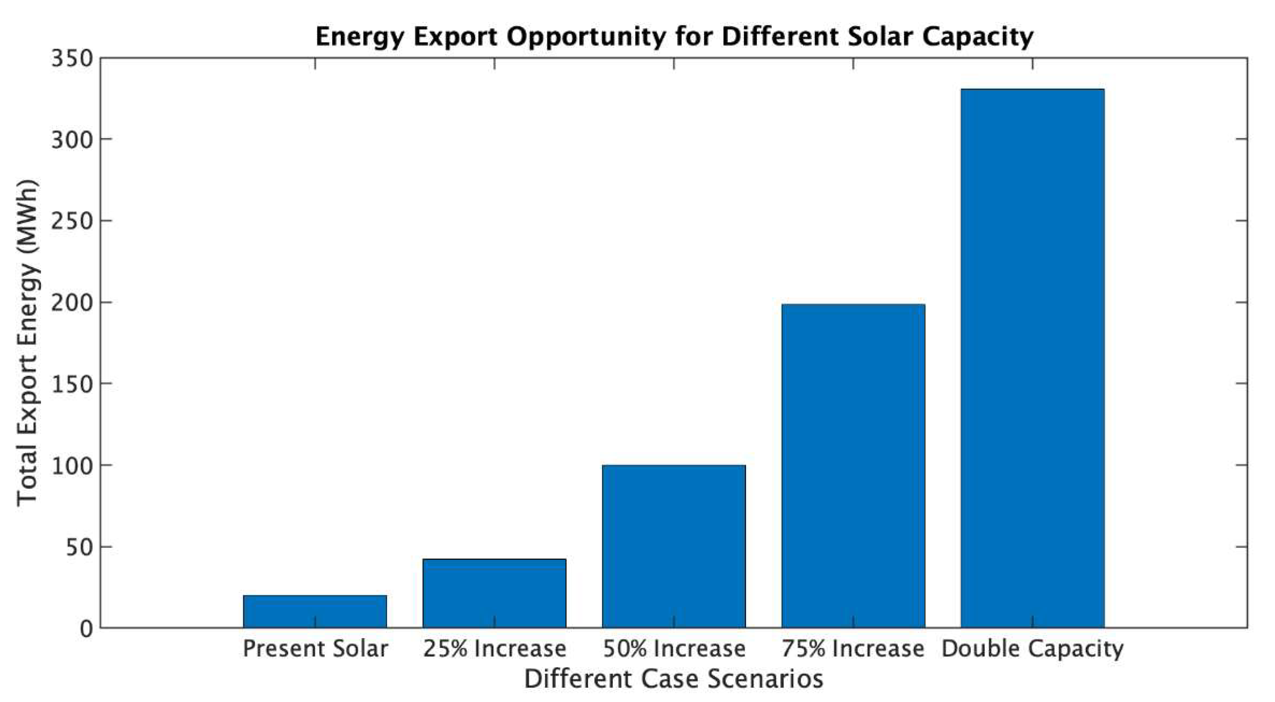
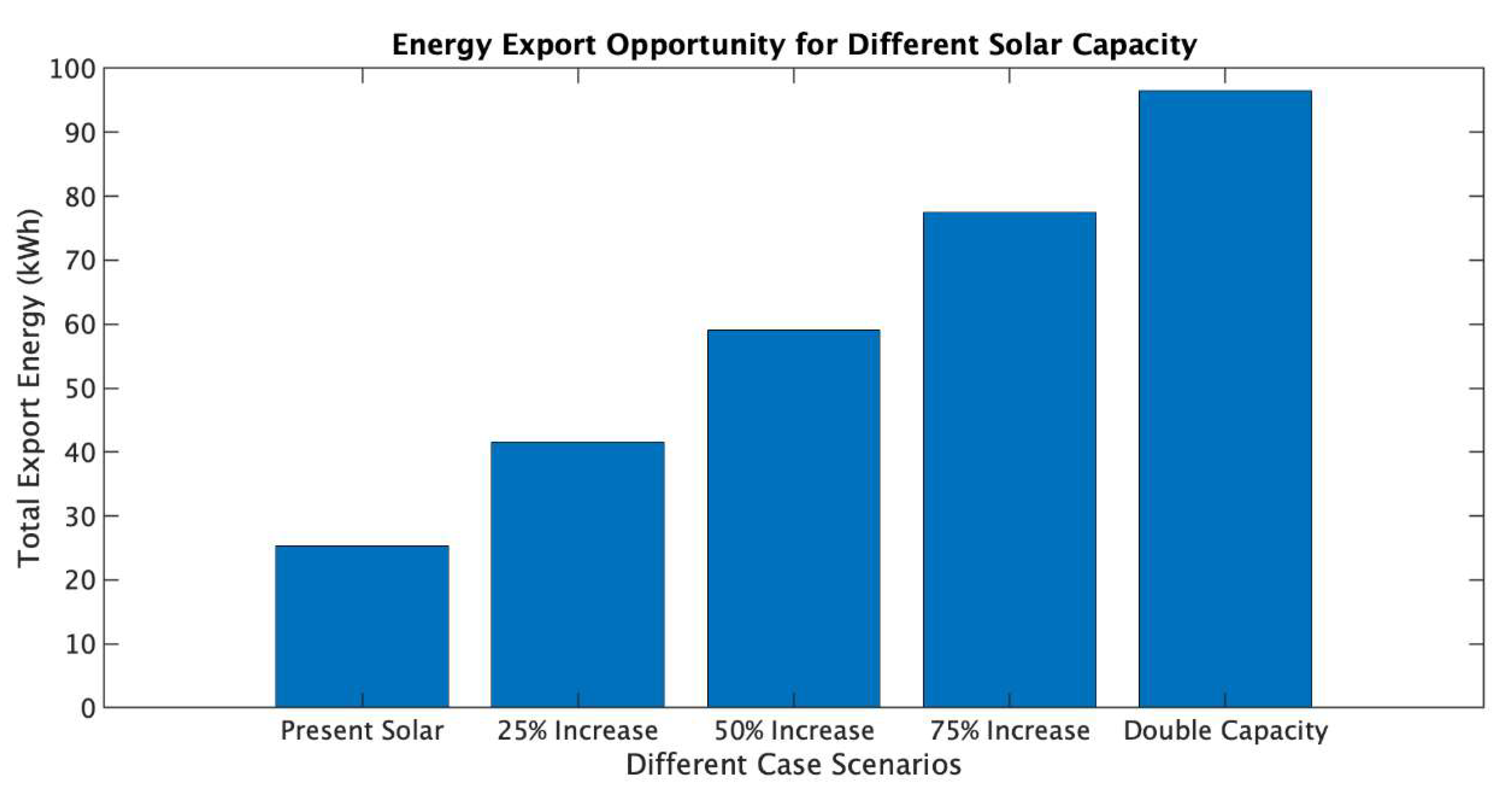
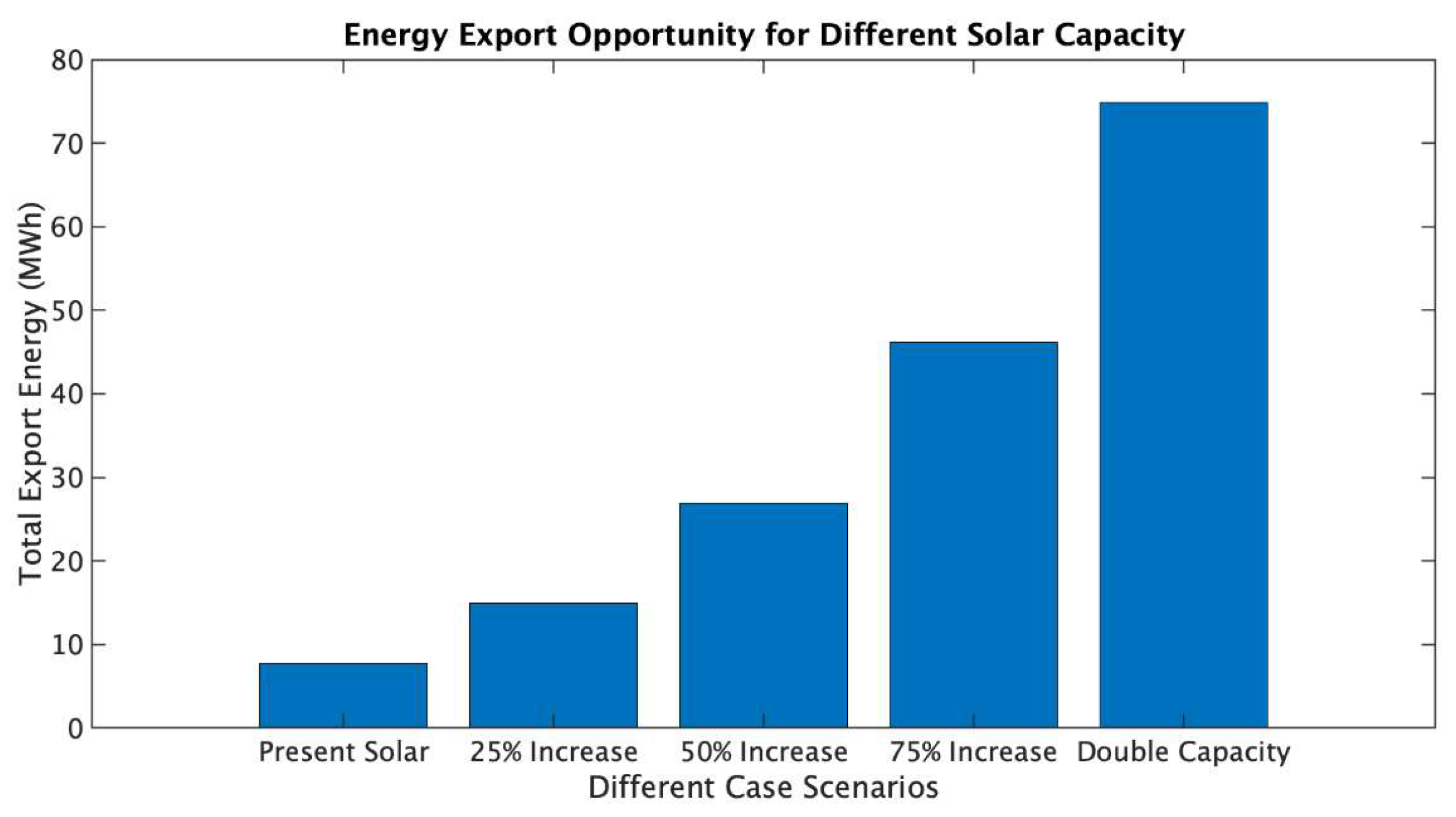
3.3.2. Opportunity Assessment: Using Solar and Energy Storage

Opportunities for using solar and battery storage were analyzed for sites A1, B1, and B2 by using their current and upcoming PV solar projects. Solar capacity data were unavailable for B3. Since the B3 pumping station had no PV solar opportunity assessment, B3 was excluded from the opportunity assessment study. The solar power generation data for 2018 and 2019 were simulated using the SAM software model from NREL. The required weather data for SAM were gathered from the NREL National Solar Radiation Database (NSRDB).

Site A1

The water utility site A1 had an 1100 kWp solar farm under construction during this study. Therefore, simulated solar generation data were used for the opportunity assessment. The optimized battery size of this site was obtained using the SAM software tool. This tool enables techno-economic optimization based on site-specific load profiles, solar generation data, and electricity tariff structures. The size of the battery was 812.726 kWh with a power rating of 162.522 kW. The optimal battery storage capacities were determined based on the site’s location, installed solar PV capacity, and the corresponding energy demand profile. The cost–benefit analysis incorporated key financial parameters for both the PV and battery energy storage system (BESS), including capital costs, replacement costs, and operation and maintenance (O&M) expenses, as detailed in

Table 5. PV and BESS financial parameters.

	Direct Capital Cost	O&M Cost	Lifetime (Year)	Inflation Rate	Discount Rate
PV	700 AUD/kW	10 AUD/kW/year	25	2.5%/year	6.4%/year
BESS	370 AUD/kWh, 270 AUD/kW	15 AUD/kWh/year	10

. A project life cycle of 25 years was assumed for the economic evaluation. Other parameters such as sales tax, installation labor, etc., were considered as business-as-usual and provided in the SAM software tool. Similar parameters were used for sites B1 and B2.

The PV–BESS model of the A1 site was simulated using the retail price. The Net Present Value (NPV) was AUD 220,072 and the simple payback period was ~10 years. The round-trip efficiency of the battery was 88.16%. The payback period was reduced to ~8 years when the wholesale tariff was used.

The total export capacity for different solar storage levels was calculated and is presented in Figure 9. A significant rise in energy export potential was observed with the increase in solar capacity.

The solar export price was lower than the NEM electricity price. One potential solution was to use battery storage to store excess energy during the daytime and utilize it during peak hours. This study considered two cases to calculate the savings related to solar energy usage. The first case exported the excess energy during the daytime and the second case stored the excess energy in battery storage and utilized it during peak hours. The return on energy export in Australia varies depending on the state and utility companies, with prices ranging from 85 AUD/MWh to 100 AUD/MWh, mostly in the upper range. However, each state has a recommended offering price, and in Victoria, the recommended price or Victorian Default Offer (VDO) is 100 AUD/MWh. Note that VDO is different from the minimum feed-in tariff, which is lower than the retail tariff [59]. To be representative, we chose 100 AUD/MWh in this study. It was assumed that the excess energy during the daytime would be stored in batteries and used during peak hours. The average peak electricity price was considered to be 165 AUD/MWh. The savings for both cases (exporting to the grid and using battery storage) in AUD are shown in

Table 6. Total energy savings during daytime with various solar capacities (A1).

Percent Solar Increase	Export to the Grid (MWh)	Savings by Exporting to the Grid (AUD)	Savings by Using Battery Storage (AUD)
Present capacity	20.40	2019	3365
25% increase	42.25	4182	6970
50% increase	99.88	9888	16,480
75% increase	198.49	19,650	32,751
100% increase	330.91	32,760	54,600

. With double the solar capacity and the use of battery storage, savings could reach AUD 54,600 in 2018, nearly AUD 22,000 more than exporting to the grid.

Site B1

The water utility site B1 had a 66 kWp solar farm operating from the end of 2019. Therefore, simulated solar generation data were used for the opportunity assessment for the year 2018. The optimized battery size of this site was obtained using the SAM software tool. The optimized battery capacity was 228.79 kWh and the battery power was 73 kW. All PV and BESS modeling parameters were kept consistent with those used for site A1. The PV–BESS model of site B1 was simulated using the retail price. The Net Present Value (NPV) was AUD 9500 and the simple payback period was ~12 years. The round-trip efficiency of the battery was 91.04%. The pay-back period was reduced to ~11 years when the wholesale tariff was used.

As seen in Figure 10, the amount of export energy increased with the increase in solar generation capacity. The total energy consumed by B1 was 180.89 MWh in 2018 and projected/simulated solar generation from the present solar farm in 2018 was 84.24 MWh. However, doubling the current solar generation capacity could generate 168.44 MWh in 2018, which was very close to the total energy requirement of B1.

The savings from different solar capacity levels are presented in

Table 7. Total energy savings during daytime with various solar capacities (B1).

Percent Solar Increase	Export to the Grid (MWh)	Savings by Exporting to the Grid (AUD)	Savings by Using Battery Storage (AUD)
Present capacity	25.33	2507	4178
25% increase	41.52	4110	6850
50% increase	59.05	5845	9743
75% increase	77.49	7671	12,785
100% increase	96.48	9551	15,918

. The savings achieved using battery storage were higher than those from exporting to the grid. The capital costs associated with PV and battery storage installation were not considered in the total savings calculation.

Site B2

The water utility site B2 had a 251 kWp solar farm that had been operating since 2020. Simulated solar generation data were used for the opportunity assessment for the year 2018. The optimized battery size for this site, obtained using the SAM software tool, was 503.461 kWh with a battery power of 96 kW. All PV and BESS modeling parameters were kept consistent with those used for sites A1 and B1. The PV–BESS model of site B2 was simulated using the retail price. The Net Present Value (NPV) was AUD 118,000 and the simple payback period was ~10 years. The round-trip efficiency of the battery was 90.53%. The payback period was reduced to ~8 years when the wholesale tariff was used.

The export capacity of B2 increased with the increase in solar capacity. The export capacity increment with a 25% increase in solar capacity is presented in Figure 11. The savings from exporting the excess energy to the grid and the savings from storing the excess energy in a battery and utilizing it during peak hours are given in

Table 8. Total energy savings during daytime with various solar capacities (B2).

Percent Solar Increase	Export to the Grid (MWh)	Savings by Exporting to the Grid (AUD)	Savings by Using Battery Storage (AUD)
Present capacity	7.73	765	1276
25% increase	14.98	1482	2471
50% increase	26.95	2667	4446
75% increase	46.15	4569	7615
100% increase	74.89	7413	12,356

. After a 100% increase in solar capacity, the total annual savings using battery storage were AUD 12,356, while the savings from exporting to the grid were AUD 7413.

4. Conclusions

This paper explored DR participation, load flexibility, and renewable energy integration in regional Australian water industries to enhance cost efficiency and sustainability. DR mechanisms improve the economic operation of water utilities by optimizing energy use during off-peak hours. Analyzing operational data from four regional sites of two Australian Water Utilities, significant potential for peak-load shifting and battery storage to reduce energy costs was identified. With 20% load shifting, electricity bill savings were AUD 60,697, AUD 1037, AUD 12,082, and AUD 6448 for sites A1, B1, B2, and B3, respectively. In addition, the results showed that integrating onsite renewable energy, particularly solar PV with battery storage, led to higher cost savings compared to grid dependency. For instance, additional savings from site A1 after integrating storage with existing PV were AUD 54,600. The Net Present Value (NPV) was AUD 220,072 and the simple payback period was ~10 years. Similarly, additional savings from B1 and B2 were AUD 15,918 and AUD 12,356, respectively. Key findings from the case studies are listed below.

• The energy and load profiles were characterized, revealing that most regional sites relied heavily on grid electricity.
• Three of the sites transitioned from an uneconomical state (EEI of more than one) to an economical state after a 5% peak load shift. The EEI values of one site remained above one even after a 20% peak load shift.
• Total savings increased by up to 60% with a 100% increase in PV with the existing battery size as the excess electricity could be utilized during peak hours rather than being exported to the grid.

The findings provide valuable insights for water utility operators, policymakers, and researchers by demonstrating effective energy management strategies that enhance sustainability while reducing costs. Future work should focus on expanding renewable energy options beyond solar PV, incorporating AI-driven predictive models for load forecasting, and evaluating the long-term financial benefits of DR participation. This paper contributes to the ongoing efforts to make regional water industries more resilient and energy-efficient, supporting the broader transition toward a sustainable energy future.

References

1. Yan, G.; Kenway, S.J.; Lam, K.L.; Lant, P.A. Water-Energy Trajectories for Urban Water and Wastewater Reveal the Impact of City Strategies. Appl. Energy 2024, 366, 123292. [Google Scholar] [CrossRef]
2. International Energy Agency. Introduction to the Water-Energy Nexus. Available online: https://www.iea.org/articles/introduction-to-the-water-energy-nexus (accessed on 30 January 2025).
3. Capodaglio, A.G. Energy Use and Decarbonisation of the Water Sector: A Comprehensive Review of Issues, Approaches, and Technological Options. Environ. Technol. Rev. 2025, 14, 40–68. [Google Scholar] [CrossRef]
4. Hasan, K.N.; Court, D.; Curtis, R.; Kashyap, S.; Jankovic, S.; Asayhe, A.; AlAbdali, A.; Anastassiou, M. Operating Cost Reduction by Electricity Profiling and Demand Management. Water Pract. Technol. 2020, 15, 921–931. [Google Scholar] [CrossRef]
5. Yasmin, R.; Amin, B.M.R.; Shah, R.; Barton, A. A Survey of Commercial and Industrial Demand Response Flexibility with Energy Storage Systems and Renewable Energy. Sustainability 2024, 16, 731. [Google Scholar] [CrossRef]
6. Amin, B.M.R.; Shah, R.; Hasan, K.N.; Tayab, U.B.; Islam, S. An Overview of Demand Response Opportunities for Commercial and Industrial Customers in the Australian NEM. In Proceedings of the 2022 IEEE PES 14th Asia-Pacific Power and Energy Engineering Conference (APPEEC), Melbourne, Australia, 20–23 November 2022; pp. 1–6. [Google Scholar]
7. Zohrabian, A.; Plata, S.L.; Kim, D.M.; Childress, A.E.; Sanders, K.T. Leveraging the Water-Energy Nexus to Derive Benefits for the Electric Grid Through Demand-Side Management in the Water Supply and Wastewater Sectors. WIREs Water 2021, 8, e1510. [Google Scholar] [CrossRef]
8. Van den Berg, C.; Danilenko, A.; World Bank. The IBNET Water Supply and Sanitation Performance Blue Book: The International Benchmarking Network for Water and Sanitation Utilities Databook; World Bank: Washington, DC, USA, 2011; 152p. [Google Scholar]
9. Kenway, S.J.; Priestley, A.; Cook, S.; Seo, M.; Inman, A.; Gregory, A.; Hall, M. Energy Use in the Provision and Consumption of Urban Water in Australia and New Zealand; Water Services Association of Australia: Docklands, Australia, 2008. [Google Scholar]
10. EPA—Environment Protection Authority. Where Do We Get Our Water? Available online: https://www.epa.sa.gov.au/soe-2018/inland-waters/where-do-we-get-our-water (accessed on 31 January 2025).
11. Melbourne Water. Natural and Urban Water Cycle. Available online: https://www.melbournewater.com.au/education/community-resources/water-knowledge/natural-and-urban-water-cycle (accessed on 31 January 2025).
12. Kizhisseri, M.I.; Mohamed, M.M.; Hamouda, M.A. A Mixed-Integer Optimization Model for Water Sector Planning and Policy Making in Arid Regions. Water Resour. Ind. 2022, 28, 100193. [Google Scholar] [CrossRef]
13. Wabela, K.; Hammani, A.; Abdelilah, T.; Tekleab, S.; El-Ayachi, M. Optimization of Irrigation Scheduling for Improved Irrigation Water Management in Bilate Watershed, Rift Valley, Ethiopia. Water 2022, 14, 3960. [Google Scholar] [CrossRef]
14. Tang, H.L.; Feng, J.; Zhou, S.Y. Reservoir Optimization Scheduling Driven by Knowledge Graphs. Electronics 2024, 13, 2283. [Google Scholar] [CrossRef]
15. Infrastructure Australia. An Assessment of Australia’s Future Infrastructure Needs; Infrastructure Australia: Forrest, Australia, 2019. [Google Scholar]
16. Beca Consultants Pty Ltd. Opportunities for Renewable Energy in the Australian Water Sector; Beca Consultants Pty Ltd.: Melbourne, Australia, 2015. [Google Scholar]
17. Bolognesi, A.; Bragalli, C.; Lenzi, C.; Artina, S. Energy Efficiency Optimization in Water Distribution Systems. Procedia Eng. 2014, 70, 181–190. [Google Scholar] [CrossRef]
18. Frijns, J.; Middleton, R.; Uijterlinde, C.; Wheale, G. Energy Efficiency in the European Water Industry: Learning from Best Practices. J. Water Clim. Change 2012, 3, 11–17. [Google Scholar] [CrossRef]
19. Zhao, Y.; Liang, B.; Shaobo, D.; Ronnie, T.; Yang, W.; Fang, C.; George, M.; Tin, H.; Vitanage, D.; Corinna, D. Energy Saving Optimisation for Water Distribution Networks—Applying Intelligent Network Optimisation Models. Water E-J. 2019, 4, 1–9. [Google Scholar] [CrossRef]
20. Strazzabosco, A.; Conrad, S.A.; Lant, P.A.; Kenway, S.J. Expert Opinion on Influential Factors Driving Renewable Energy Adoption in the Water Industry. Renew. Energy 2020, 162, 754–765. [Google Scholar] [CrossRef]
21. Sowby, R.B. Increasing water and wastewater utility participation in demand response programs. Energy Nexus 2021, 1, 100001. [Google Scholar] [CrossRef]
22. Martin-Candilejo, A.; Santillán, D.; Garrote, L. Pump Efficiency Analysis for Proper Energy Assessment in Optimization of Water Supply Systems. Water 2020, 12, 132. [Google Scholar] [CrossRef]
23. Skoczko, I. Energy Efficiency Analysis of Water Treatment Plants: Current Status and Future Trends. Energies 2025, 18, 1086. [Google Scholar] [CrossRef]
24. Melbourne Water. Melbourne Water Annual Report 2003/2004; Melbourne Water: Melbourne, Australia, 2004. [Google Scholar]
25. Strazzabosco, A.; Kenway, S.J.; Lant, P.A. Quantification of Renewable Electricity Generation in the Australian Water Industry. J. Clean. Prod. 2020, 254, 120119. [Google Scholar] [CrossRef]
26. Strazzabosco, A.; Kenway, S.J.; Conrad, S.A.; Lant, P.A. Renewable Electricity Generation in the Australian Water Industry: Lessons Learned and Challenges for the Future. Renew. Sust. Energy Rev. 2021, 147, 111236. [Google Scholar] [CrossRef]
27. Grieser, B.; Sunak, Y.; Madlener, R. Economics of Small Wind Turbines in Urban Settings: An Empirical Investigation for Germany. Renew. Energy 2015, 78, 334–350. [Google Scholar] [CrossRef]
28. Lopes, R.A.; Junker, R.G.; Martins, J.; Murta-Pina, J.; Reynders, G.; Madsen, H. Characterisation and Use of Energy Flexibility in Water Pumping and Storage Systems. Appl. Energy 2020, 277, 115587. [Google Scholar] [CrossRef]
29. Zakariazadeh, A.; Ahshan, R.; Al Abri, R.; Al-Abri, M. Renewable Energy Integration in Sustainable Water Systems: A Review. Clean. Eng. Technol. 2024, 18, 100722. [Google Scholar] [CrossRef]
30. Sharifzadeh, M.; Hien, R.K.T.; Shah, N. China’s Roadmap to Low-Carbon Electricity and Water: Disentangling Greenhouse Gas (GHG) Emissions from Electricity-Water Nexus via Renewable Wind and Solar Power Generation, and Carbon Capture and Storage. Appl. Energy 2019, 235, 31–42. [Google Scholar] [CrossRef]
31. Skroufouta, S.; Baltas, E. Investigation of Hybrid Renewable Energy System (HRES) for Covering Energy and Water Needs on the ISLAND of Karpathos in Aegean Sea. Renew. Energy 2021, 173, 141–150. [Google Scholar] [CrossRef]
32. Lima, D.; Appleby, G.; Li, L. A Scoping Review of Options for Increasing Biogas Production from Sewage Sludge: Challenges and Opportunities for Enhancing Energy Self-Sufficiency in Wastewater Treatment Plants. Energies 2023, 16, 2369. [Google Scholar] [CrossRef]
33. Lu, X.X.; Li, K.P.; Xu, H.C.; Wang, F.; Zhou, Z.Y.; Zhang, Y.G. Fundamentals and Business Model for Resource Aggregator of Demand Response in Electricity Markets. Energy 2020, 204, 117885. [Google Scholar] [CrossRef]
34. Tadokoro, H.; Koibuchi, H.; Takahashi, S.; Kakudou, S.; Takata, Y.; Moriya, D.; Sasakawa, M. Water Supply Control System for Smarter Electricity Power Usage Adopting Demand-Response Scheme. Water Supply 2020, 20, 140–147. [Google Scholar] [CrossRef]
35. Menke, R.; Abraham, E.; Parpas, P.; Stoianov, I. Demonstrating Demand Response from Water Distribution System Through Pump Scheduling. Appl. Energy 2016, 170, 377–387. [Google Scholar] [CrossRef]
36. Chitsaz, H.; Zamani-Dehkordi, P.; Zareipour, H.; Parikh, P.P. Electricity Price Forecasting for Operational Scheduling of Behind-the-Meter Storage Systems. IEEE Trans. Smart Grid 2018, 9, 6612–6622. [Google Scholar] [CrossRef]
37. Fang, D.L.; Chen, B. Linkage Analysis for the Water-Energy Nexus of City. Appl. Energy 2017, 189, 770–779. [Google Scholar] [CrossRef]
38. Chen, S.Q.; Chen, B. Urban Energy-Water Nexus: A Network Perspective. Appl. Energy 2016, 184, 905–914. [Google Scholar] [CrossRef]
39. Patrick, A.O. The $16 Billion Plan to Beam Australia’s Outback Sun Onto Asia’s Power Grids. 2020. Available online: https://www.washingtonpost.com/climate-solutions/2020/08/10/australia-solar-energy-asia/ (accessed on 31 January 2025).
40. Harrou, F.; Dairi, A.; Dorbane, A.; Sun, Y. Energy Consumption Prediction in Water Treatment Plants Using Deep Learning with Data Augmentation. Results Eng. 2023, 20, 101428. [Google Scholar] [CrossRef]
41. Oulebsir, R.; Lefkir, A.; Safri, A.; Bermad, A. Optimization of the Energy Consumption in Activated Sludge Process Using Deep Learning Selective Modeling. Biomass BioEnergy 2020, 132, 105420. [Google Scholar] [CrossRef]
42. Zairi, S.; Meddah, B.; Slimani, M. Optimisation of the Energy Consumption in Activated Sludge Treatment Plants Using Simulation Model. Int. J. Environ. Pollut. 2024, 74, 198–231. [Google Scholar] [CrossRef]
43. Adibimanesh, B.; Polesek-Karczewska, S.; Bagherzadeh, F.; Szczuko, P.; Shafighfard, T. Energy Consumption Optimization in Wastewater Treatment Plants: Machine Learning for Monitoring Incineration of Sewage Sludge. Sustain. Energy Technol. 2023, 56, 103040. [Google Scholar] [CrossRef]
44. Li, Z.H.; Zou, Z.H.; Wang, L.P. Analysis and Forecasting of the Energy Consumption in Wastewater Treatment Plant. Math. Probl. Eng. 2019, 2019, 8690898. [Google Scholar] [CrossRef]
45. Harrou, F.; Cheng, T.Y.; Sun, Y.; Leiknes, T.; Ghaffour, N. A Data-Driven Soft Sensor to Forecast Energy Consumption in Wastewater Treatment Plants: A Case Study. IEEE Sens. J. 2021, 21, 4908–4917. [Google Scholar] [CrossRef]
46. Zylka, R.; Dabrowski, W.; Malinowski, P.; Karolinczak, B. Modeling of Electric Energy Consumption During Dairy Wastewater Treatment Plant Operation. Energies 2020, 13, 3769. [Google Scholar] [CrossRef]
47. Cheng, T.Y.; Harrou, F.; Kadri, F.; Sun, Y.; Leiknes, T. Forecasting of Wastewater Treatment Plant Key Features Using Deep Learning-Based Models: A Case Study. IEEE Access 2020, 8, 184475–184485. [Google Scholar] [CrossRef]
48. Bagherzadeh, F.; Nouri, A.S.; Mehrani, M.J.; Thennadil, S. Prediction of Energy Consumption and Evaluation of Affecting Factors in a Full-Scale WWTP Using a Machine Learning Approach. Process Saf. Environ. 2021, 154, 458–466. [Google Scholar] [CrossRef]
49. Alekseev, A.V. Study of the Forecasting Problem of Energy Consumption of Water Pumping Station. E3S Web Conf. 2019, 102, 03001. [Google Scholar] [CrossRef]
50. SILO. Australian Climate Data from 1889 to Yesterday. Available online: https://www.longpaddock.qld.gov.au/silo/ (accessed on 31 January 2025).
51. NREL. Available online: https://www.nrel.gov/ (accessed on 31 January 2025).
52. Bureau of Meteorology. Water Data Transfer Format (WDTF). Available online: http://www.bom.gov.au/water/standards/wdtf/ (accessed on 31 January 2025).
53. FIWARE. Smart Cities. Available online: https://www.fiware.org/ (accessed on 31 January 2025).
54. Li, C.B.; Tang, S.W.; Cao, Y.J.; Xu, Y.J.; Li, Y.; Li, J.X.; Zhang, R.S. A New Stepwise Power Tariff Model and Its Application for Residential Consumers in Regulated Electricity Markets. IEEE Trans. Power Syst. 2013, 28, 300–308. [Google Scholar] [CrossRef]
55. AEMO. Available online: https://aemo.com.au/en (accessed on 31 January 2025).
56. Ram, B. Tariffs and Load Management—A Post, Privatisation Study of the UK Electricity Supply Industry. IEEE Trans. Power Syst. 1995, 10, 1111–1117. [Google Scholar] [CrossRef]
57. Mcrae, M.R.; Scheer, R.M.; Smith, B.A. Integrating Load Management Programs into Utility Operations and Planning with a Load Reduction Forecasting System. IEEE Trans. Power Appar. Syst. 1985, 104, 1321–1325. [Google Scholar] [CrossRef]
58. Palensky, P.; Dietrich, D. Demand Side Management: Demand Response, Intelligent Energy Systems, and Smart Loads. IEEE Trans. Ind. Inform. 2011, 7, 381–388. [Google Scholar] [CrossRef]
59. ESC. Available online: https://www.esc.vic.gov.au/electricity-and-gas/prices-tariffs-and-benchmarks/minimum-feed-tariff/minimum-feed-tariff-review-2021-22 (accessed on 31 January 2025).
Figure 1. The amount of electricity consumption in the water sector from 2014 to 2040.
Sustainability 17 03364 g001
Figure 2. Data analytical steps for energy mapping and feature selection.
Sustainability 17 03364 g002
Figure 3. Data cleaning process and how it related to feature engineering.
Sustainability 17 03364 g003
Figure 4. Wholesale and retail tariff variation over a week: (a) Australian NEM electricity spot price variation in Victoria (23–29 July 2018) and (b) Retail electricity price.
Sustainability 17 03364 g004
Figure 5. Overall data analytical methodology for data analyses and DR opportunity assessment in the regional water industry.
Sustainability 17 03364 g005
Figure 6. Barriers and challenges in data acquisition and processing in water industries.
Sustainability 17 03364 g006
Figure 7. Electrical energy consumption pattern: (a) site A1; (b) site B1; (c) site B2; (d) site B3.
Sustainability 17 03364 g007
Figure 8. Savings after load shifting considering retail electricity price: (a) site A; (b) site B1; (c) site B2; (d) site B3.
Sustainability 17 03364 g008
Figure 9. Total energy export potential at different levels of solar capacity for utility site A1.
Sustainability 17 03364 g009
Figure 10. Total energy export potential at different levels of solar capacity for utility site B1.
Sustainability 17 03364 g010
Figure 11. Total energy export potential at different levels of solar capacity increase in B2.
Sustainability 17 03364 g011