Ecological Stress Assessment on Vegetation in the Al-Baha Highlands, Saudi Arabia (1991–2023)

Abstract

Climate change significantly stresses cold-adapted and stenothermic plant species in high-altitude mountain ecosystems. The diverse plant species at elevations ranging from 1324 to 2527 m above mean sea level (AMSL) provide an ideal setting for investigating these impacts in the Al-Baha Highlands, Saudi Arabia. Therefore, this study has three aims: first, to estimate vegetation cover in 2023 and its relationship with environmental factors; second, to analyze long-term trends (1991–2023) in key spectral indices, including the normalized difference vegetation index (NDVI), normalized difference vegetation water index (NDWI), normalized difference open water index (NDWIw), and land surface temperature (LST), using the Kendall tau-b method; and third, to model ecological stress via a generalized additive model (GAM) and assess its impact on vegetation. We utilized Landsat 5/7/8 (C2 SR T1) for spectral indices and the Copernicus DEM for topographic and hydrological analysis. The results indicate significant roles of LST, elevation, and distance from seasonal streams in shaping vegetation patterns (p < 2 × 10⁻¹⁶). There were negative trends in the NDVI (91.66 km²), NDWI (138 km²), and NDWIw (804 km²) (p < 0.05), whereas the LST exhibited positive trends (116.15 km²) (p < 0.05). The GAM achieved high predictive accuracy (R² = 0.979), capturing nonlinear relationships between the predictors and the stress score. Severe ecological stress occurred in high-altitude zones (>1700 m AMSL) on south-facing slopes due to increased LST and declining NDWI, impacting species such as Juniperus procera. Hypothesis testing was used to assess variations in the NDVI, its long-term trends, and ecological stress between highland and lower-elevation areas, revealing highly significant differences (p < 2.2 × 10⁻¹⁶). This study provides novel insights into ecological stress dynamics in relation to altitude and slope aspects, offering actionable recommendations for sustainable ecosystem management, including targeted reforestation and water resource optimization to mitigate stress and preserve biodiversity.

1. Introduction

Climate change significantly threatens tropical and subtropical high mountain plant species [1] by causing range shifts to higher elevations, which increases the risk of local extinction for endemic species [2]. It also facilitates the establishment of invasive species, disrupts phenological events affecting plant–pollinator interactions, and contributes to habitat loss and fragmentation [3]. The Al-Baha Highlands also face species migration, local extinctions, invasive threats, disrupted plant–pollinator interactions, and habitat loss due to climate change [4]. These highlands receive relatively high amounts of rainfall due to orographic lifting, making them home to diverse vegetation, including Maytenus parviflora (Loes.) Cufod. (Celastrales: Celastraceae), Juniperus procera Hochst. ex Endl. (Pinales: Cupressaceae), Lavandula dentata L. (Lamiales: Lamiaceae), Themeda triandra Forssk. (Poales: Poaceae), Barbeya oleoides Schweinf. (Rosales: Barbeyaceae), and Olea europaea L. (Lamiales: Oleaceae) [5]. The presence of rare and endemic species such as Periploca somalensis Browicz (Gentianales: Apocynaceae), Celtis tournefortii Lam. (Rosales: Cannabaceae), and Kleinia odora (Forssk.) DC. (Asterales: Asteraceae) [6] further underscores the ecological significance and conservation value of this region.

The Al-Baha Highlands are currently experiencing increasing ecological stress due to the effects of climate change [7]. Rising temperatures [8,9] lead to habitat degradation and shifts in vegetation dynamics. These changes pose a significant threat to the unique flora of the highlands [10].

Several studies have explored vegetation dynamics and ecological stress by employing remote sensing and ecological modeling techniques. Researchers have utilized vegetation indices such as the normalized difference vegetation index (NDVI) [11,12] and water indices such as the normalized difference water index (NDWI) to monitor vegetation health and water availability [13,14]. Similarly, land surface temperature (LST) has been widely used to assess the effects of thermal stress on ecosystems [15]. Trend analysis methods such as Kendall tau [16] and Sen’s slope [17] have been used to detect temporal changes in ecological variables over time. Generalized additive models (GAMs) have been applied to study the relationships between ecological stress and the effect of spectral indices [18,19]. However, most existing studies lack specific attention to the intricate interplay between climatic, topographic, and hydrological variables in determining ecological stress in highland regions such as Al-Baha.

To address these gaps, this study adopts an integrated approach that combines long-term trend analysis, ecological modeling, and aspect analysis to assess ecological stress and its implications for vegetation in the Al-Baha Highlands.

The objectives of this watershed study are threefold: first, to estimate the extent of vegetation cover and its relationship with elevation, temperature, proximity to seasonal streams and slope aspects; second, to calculate trends in ecological variables, including the NDVI, NDWI, NDWIw, and LST, from 1991–2023 via the use of Kendall Tau b coefficients with significance thresholds (p < 0.05); and third, to predict ecological stress by integrating these trends into a GAM model.

The watershed elevation ranges from 1323 to 2527 m AMSL, with the highland ecosystem defined as the region between 1700 and 2527 m and the lower elevation below 1700 m. To assess the relationships between elevation and vegetation, long-term NDVI trends, and ecological stress, the following hypotheses are proposed:

1.

Hypothesis on NDVI Distribution:

• Null Hypothesis (H₀): There is no significant difference in the distribution of NDVI values between highland and lower-elevation ecosystems.
• Alternative Hypothesis (H_a): There is a significant difference in the distribution of NDVI values between highland and lower-elevation ecosystems.

2.

Hypothesis on NDVI Long-Term Trends:

• Null Hypothesis (H0): The long-term trends in the NDVI are not significantly different between highland and lower-elevation ecosystems.
• Alternative Hypothesis (Ha): The long-term trends in the NDVI differ significantly between highland and lower-elevation ecosystems.

3.

Hypothesis on Ecological Stress:

• Null Hypothesis (H0): Ecological stress does not vary significantly between highland and lower-elevation ecosystems.
• Alternative Hypothesis (Ha): Ecological stress varies significantly between highland and lower-elevation ecosystems.

These hypotheses align with the study’s objectives to estimate vegetation cover, analyze trends in ecological variables, and predict ecological stress via statistical and modeling approaches. This research provides a comprehensive framework for evaluating ecological stress in highland and lower-elevation environments, offering valuable contributions to the growing body of literature on climate change impacts at different altitudes. By integrating spatial, temporal, and ecological data, this study seeks to fill knowledge gaps and inform adaptive strategies for preserving the unique biodiversity of the Al-Baha Highlands.

2. Materials and Methods

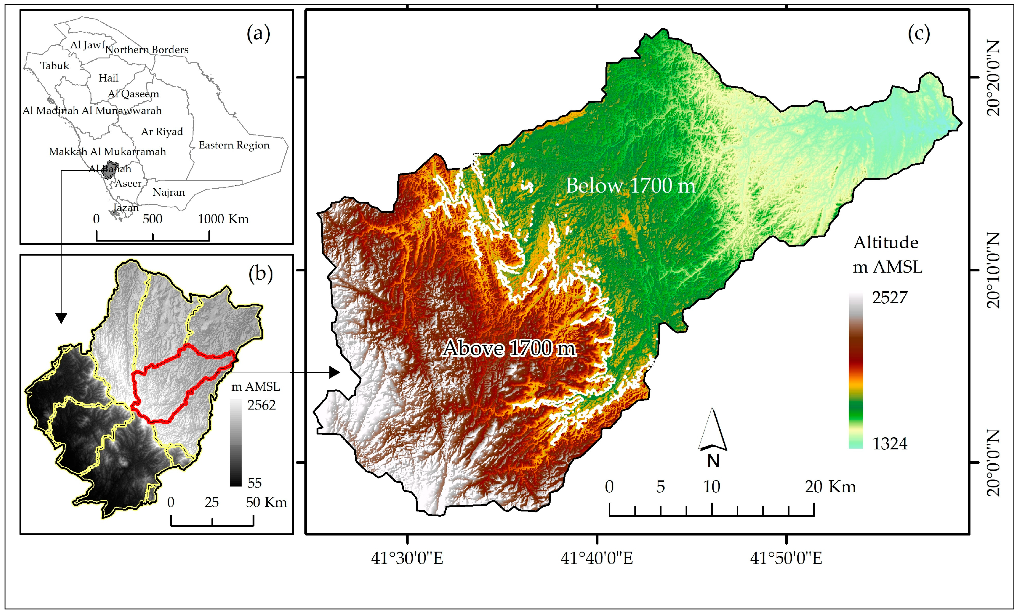
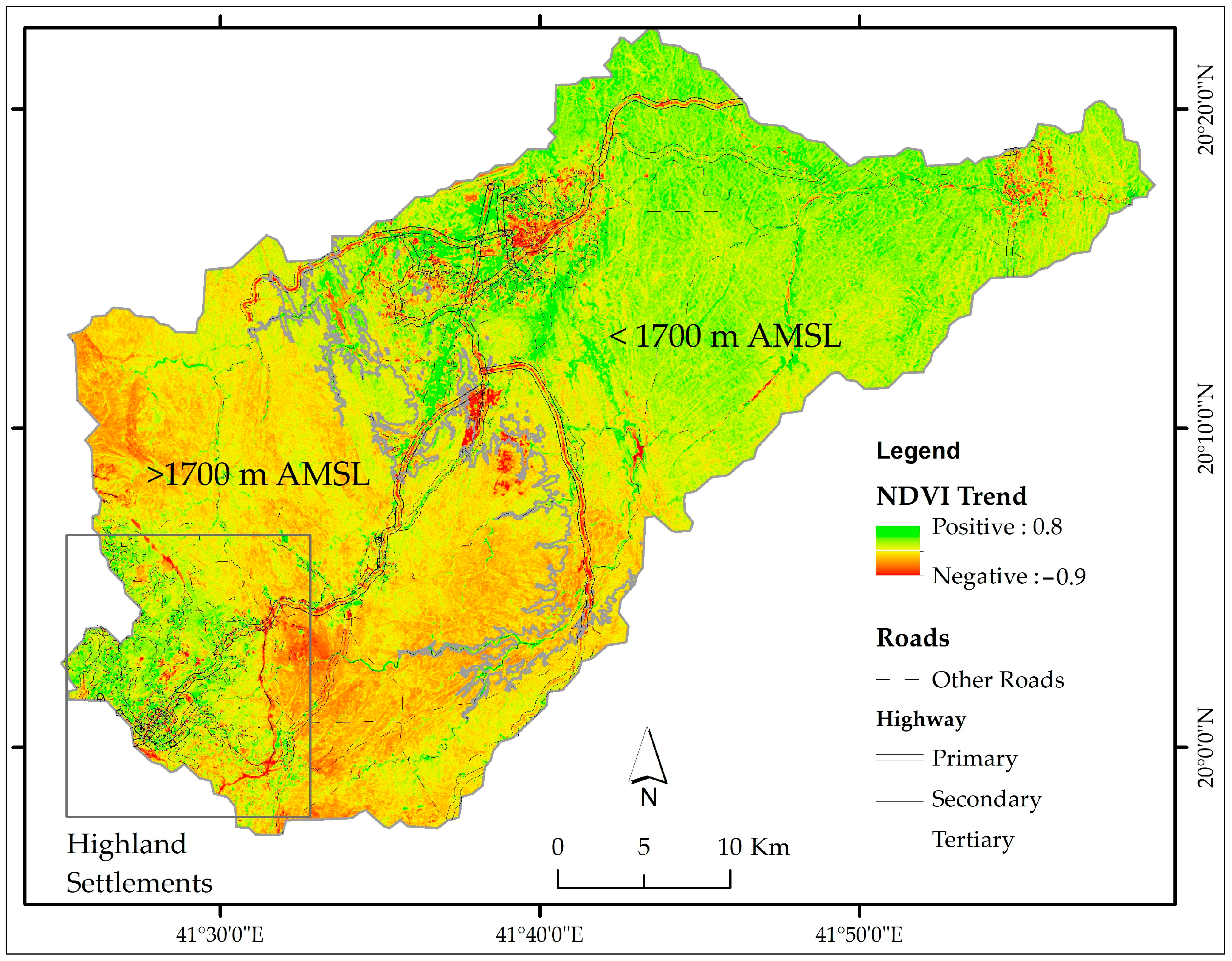
2.1. Study Area

The Al-Baha watershed spans the geographic coordinates of 19°57′–20°22′ N and 41°25′–41°59′ E (Figure 1), with a total area of approximately 1425 km².

The study area was divided into two elevation zones on the basis of a 1700 m threshold, reflecting the region’s biophysical characteristics. The high-altitude mountains (1700–2527 m) consist of undulating plateaus and peaks where vegetation is denser (up to 86% cover), with diverse woodland and shrubland species. In contrast, the eastern mountains (1300–1700 m) gradually descend towards the east and northeast, intersected by valleys, where vegetation exhibits lower species diversity and sparse cover (below 20%).

The watershed consists of microclimatic and ecological niches that influence vegetation distribution at different aspects and altitudes. The average annual temperature ranges from 12 °C to 23 °C [20], with average annual rainfall (100–200 mm) occurring primarily during the spring and summer months, supporting the region’s unique vegetation and ecological dynamics.

Figure 2 shows the trends of the annual averages of key climatic variables from 1991–2023 for the watershed, which were sourced from TerraClimate (https://www.climatologylab.org/terraclimate.html, accessed on 9 December 2024) and analyzed via interquartile ranges to remove outliers. These trends reveal indications of ecological stress. Rising maximum and minimum temperatures signify increasing thermal stress, whereas increasing minimum and mean rainfall and decreasing maximum rainfall suggest potential reductions in rainfall variability. The negative trends in actual evapotranspiration and potential water deficit further indicate hydrological imbalances. Additionally, increasing Hargreaves PET highlights the increased atmospheric demand for water, exacerbating the stress on the watershed. These variables collectively serve as sensitive indicators of climate-induced ecological stress.

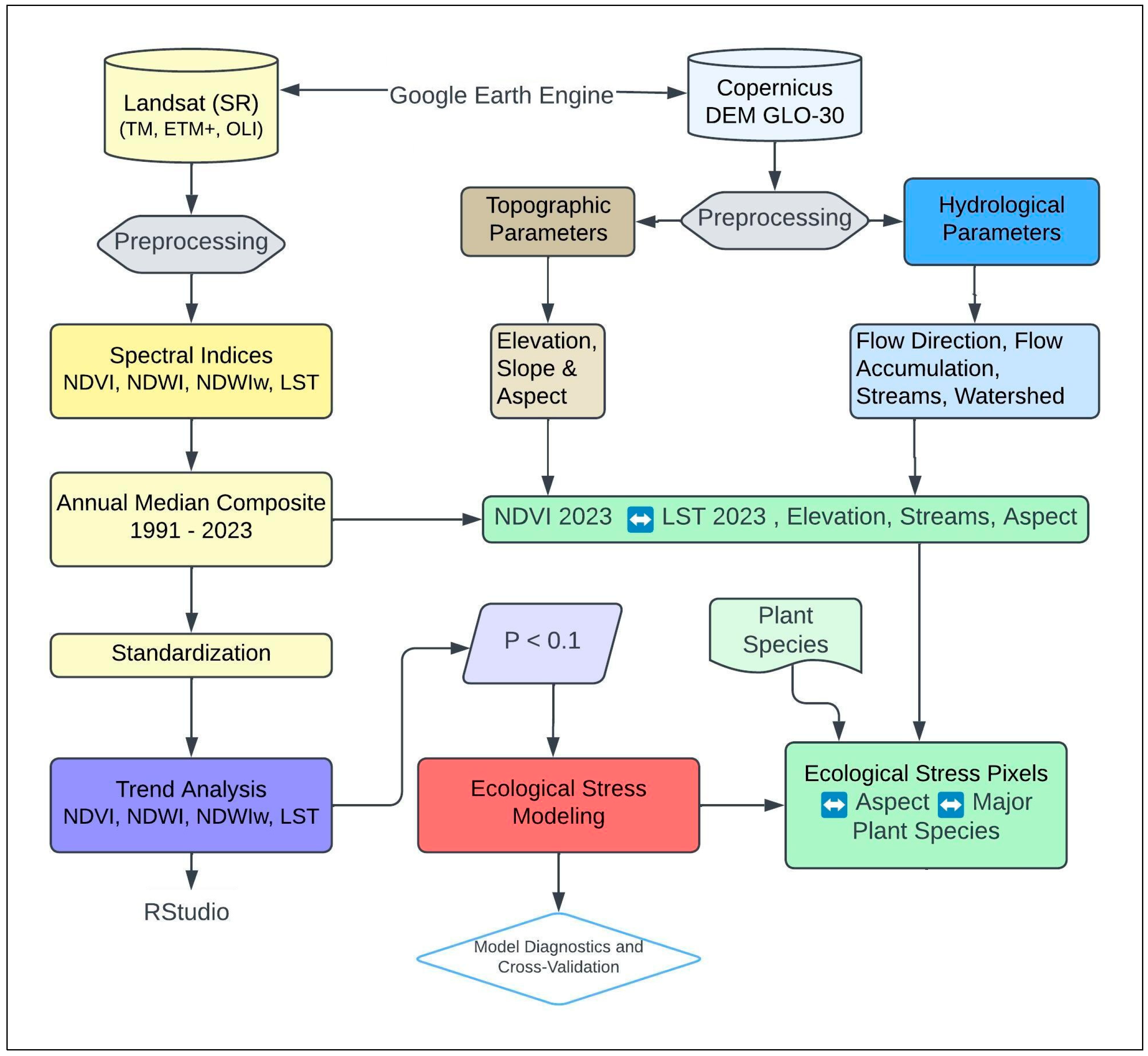
2.2. Overall Methodology

The schematic framework, illustrated in Figure 3, outlines the methodology, which consists of three main components. The first component focuses on generating annual median composites of spectral indices for the period 1991–2023 via Landsat (SR) data. The second component addresses ecological stress prediction, incorporating long-term trends of key environmental variables and, the third component ultimately evaluates the impact of ecological stress on the vegetation within the study area.

2.3. Data Used

We utilized surface reflectance (SR) products from Landsat TM, ETM+, and OLI/TIRS (https://developers.google.com/earth-engine/datasets/catalog/landsat, accessed on 10 December 2024) sensors to generate spectral indices. These Landsat products are atmospherically corrected, such as absorption and scattering, and account for illumination and viewing geometry effects, representing the highest level of processing available for Landsat data and ensuring a more accurate representation of the Earth’s surface [21]. Additionally, these products include pixel quality flags derived via the CFMask algorithm to identify conditions such as clear, water, snow, cloud, or shadow conditions. This quality information was employed to filter and select the most reliable data for each composite period, ensuring high-quality inputs for the analysis [22].

The Copernicus DEM GLO-30 (https://developers.google.com/earth-engine/datasets/catalog/COPERNICUS_DEM_GLO30, accessed on 10 December 2024), a 30 m resolution DEM [23], was utilized to derive elevation, slope, aspect, and contour lines, offering insights into terrain variability. Hydrological analysis, including flow direction, flow accumulation, stream networks, and watershed boundaries, was performed via the DEM to understand water movement patterns. Administrative boundary data were obtained from OCHA (https://data.humdata.org/dataset/cod-ab-sau, accessed on 8 December 2024).

2.4. Computation of Spectral Indices

The analysis of spectral indices was conducted via the Google Earth Engine platform, which leverages Landsat 5/7/8 surface reflectance (SR) data for the period 1991–2023.

Table 1. Spectral bands and corresponding wavelengths (in micrometers) for the green, red, near-infrared (NIR), shortwave infrared (SWIR1 and SWIR2) and thermal regions across the Landsat 5 TM, Landsat 7 ETM+, and Landsat 8 OLI sensors.

Sensor	Green (µm)	Red (µm)	NIR (µm)	SWIR1 (µm)	SWIR2 (µm)	Thermal (µm)
Landsat 5 TM	B2 (0.52–0.60)	B3 (0.63–0.69)	B4 (0.76–0.90)	B5 (1.55–1.75)	B7 (2.08–2.35)	B6 (10.40–12.50)
Landsat 7 ETM+	B2 (0.52–0.60)	B3 (0.63–0.69)	B4 (0.77–0.90)	B5 (1.55–1.75)	B7 (2.09–2.35)	B6 (10.40–12.50)
Landsat 8 OLI	B3 (0.53–0.59)	B4 (0.64–0.67)	B5 (0.85–0.88)	B6 (1.57–1.65)	B7 (2.11–2.29)	TIRS B10 (10.60–11.19)

list the spectral bands and corresponding wavelengths (in micrometers). For each year, the annual median was calculated by aggregating all observations from 1 January to 31 December. The median statistic was employed to reduce the influence of outliers caused by clouds, atmospheric noise, and extreme values. To account for sensor differences, we adjusted the Landsat 5 ETM and 7 ETM+ spectral indices to match the Landsat 8 OLI data via simple linear transformation [24].

The NDVI is used to assess the photosynthetic activity of vegetation [25]. The NDVI was calculated via Equation (1):

$$\mathrm{N}\mathrm{D}\mathrm{V}\mathrm{I}={\displaystyle \frac{\left({\mathrm{\rho }}_{\mathrm{N}\mathrm{I}\mathrm{R}}-{\mathrm{\rho }}_{\mathrm{R}\mathrm{E}\mathrm{D}}\right)}{\left({\mathrm{\rho }}_{\mathrm{N}\mathrm{I}\mathrm{R}}+{\mathrm{\rho }}_{\mathrm{R}\mathrm{E}\mathrm{D}}\right)}}$$

(1)

The NDWI was derived to obtain the vegetation liquid water content [26] via Equation (2):

$$NDWI={\displaystyle \frac{{\rho }_{NIR}}{{\rho }_{SWIR1}}}$$

(2)

NDWIw was derived to obtain the open water [27] via Equation (3):

$$\mathrm{N}\mathrm{D}\mathrm{W}\mathrm{I}\mathrm{w}={\displaystyle \frac{{\mathrm{\rho }}_{\mathrm{G}\mathrm{R}\mathrm{E}\mathrm{E}\mathrm{N}}}{{\mathrm{\rho }}_{\mathrm{S}\mathrm{W}\mathrm{I}\mathrm{R}1}}}$$

(3)

The land surface temperature (LST) was computed by first converting the raw digital number (DN) values to top-of-atmosphere (TOA) radiance through radiometric rescaling via multiplicative and additive factors. The TOA radiance was then transformed into brightness temperature (Kelvin) via Planck’s law and sensor-specific calibration constants [28]. Thereafter, the LST was calculated from the brightness temperature and emissivity [29] via Equation (4):

$$\mathrm{L}\mathrm{S}\mathrm{T}={\displaystyle \frac{\mathrm{T}\mathrm{b}}{1+\left(\mathrm{\lambda }\times \mathrm{T}\mathrm{b}/\mathrm{\rho }\right)\times \mathrm{l}\mathrm{n}\left(\mathrm{ϵ}\right)}}$$

(4)

where Tb is the brightness temperature in Kelvin; λ is the wavelength of the emitted radiance; ρ is a constant; and ϵ is the surface emissivity.

2.5. Trend Analysis

Temporal trends in the annual median spectral indices were analyzed via the nonparametric Kendall tau-b correlation coefficient [30], which is robust to nonnormal data distributions and missing values. This method assesses the direction and significance of index trends over a 32-year period.

Kendall’s tau-b rank correlation was calculated via Equation (5):

$${\mathrm{\tau }}_{\mathrm{b}}={\displaystyle \frac{\mathrm{C}-\mathrm{D}}{\sqrt{(\mathrm{C}+\mathrm{D}+{\mathrm{T}}_{\mathrm{x}})(\mathrm{C}+\mathrm{D}+{\mathrm{T}}_{\mathrm{y}})}}}$$

(5)

where C is the number of concordant pairs, D is the number of discordant pairs, T_x is the number of ties in the independent “Time” variable, and Ty is the number of ties in the dependent variables.

The Mann–Kendall (MK) test was applied to evaluate the trends [31]. Additionally, a paired t test was conducted to compare the areas of positive and negative trends across the groups, providing further statistical validation of the observed differences in the trend areas. This helped identify significant spatial differences between the trend areas.

2.6. Ecological Stress Modeling

To assess the ecological stress and effects of key variable trends, a generalized additive model (GAM) was employed to model the relationships between the environmental variables and stress scores [32].

2.6.1. Stress Score

The stress score was calculated by applying p-value masking (p < 0.1) to exclude statistically insignificant trends. The trend values (τ) were weighted on the basis of stress direction, with negative trends (e.g., NDVI, NDWI, and NDWIw) calculated as −τ⋅W and positive trends (e.g., LST) calculated as τ⋅W, where W represents variable-specific weights, Equation (6).

$${\mathrm{Stress}}_i=-{\tau }_i\cdot W_i(-\mathrm{trend}, \mathrm{NDVI}, \mathrm{NDWI}, \mathrm{NDWIw}) \mathrm{or} {\tau }_i\cdot W_i(+\mathrm{trend}, \mathrm{LST})$$

(6)

Individual stress rasters were subsequently combined into a composite ecological stress raster by summing the weighted stress values, ignoring the NA values to ensure accurate aggregation, Equation (7).

$$\mathrm{Composite} \mathrm{Stress}={\displaystyle \sum _{i=1}^n}{\mathrm{Stress}}_i$$

(7)

2.6.2. Stress Modeling

This stress score was normalized for subsequent analysis. The GAM model was defined to incorporate smooth terms for each predictor via thin plate regression splines (bs = “tp”) with a knot value of 10. The final GAM model is represented via Equation (8):

$$\begin{array}{cc}\hfill \mathrm{E}\mathrm{c}\mathrm{o}\mathrm{l}\mathrm{o}\mathrm{g}\mathrm{i}\mathrm{c}\mathrm{a}\mathrm{l}\mathrm{s}\mathrm{t}\mathrm{r}\mathrm{e}\mathrm{s}\mathrm{s}& \sim \mathrm{s}\left(\mathrm{\tau }\mathrm{L}\mathrm{S}\mathrm{T},\mathrm{b}\mathrm{s}=\mathrm{tp},\mathrm{k}=10\right)+\mathrm{s}\left(\mathrm{\tau }\mathrm{N}\mathrm{D}\mathrm{W}\mathrm{I},\mathrm{b}\mathrm{s}=\mathrm{tp},\mathrm{k}=10\right)\hfill \\ & +\mathrm{s}\left(\mathrm{\tau }\mathrm{N}\mathrm{D}\mathrm{V}\mathrm{I},\mathrm{b}\mathrm{s}=\mathrm{tp},\mathrm{k}=10\right)+\mathrm{s}\left(\mathrm{\tau }\mathrm{N}\mathrm{D}\mathrm{W}\mathrm{I}\mathrm{w},\mathrm{b}\mathrm{s}=\mathrm{tp},\mathrm{k}=10\right)\hfill \end{array}$$

(8)

Here, thin plate splines (bs = “tp”) with 10 knots (k = 10) are applied to the Kendall tau-b trends of the NDVI, LST, NDWI, and NDWIw. This allows the model to capture the nonlinear relationships between these predictors and the stress score, providing flexibility without overfitting.

The GAM was fitted via the mgcv package in R [33]. Model residuals were evaluated via diagnostic plots to ensure that the assumptions of the model were met. The model’s predictive performance was assessed via linear regression between the observed and predicted stress scores. To further evaluate the model’s robustness and predictive accuracy, a 10-fold cross-validation approach was employed [34]. Residual diagnostics, including the computation of residuals and standardized residuals, were conducted to assess the model’s performance comprehensively. Spatial autocorrelation was examined via Moran’s I [35] to identify clustering patterns in the GAM-predicted stress scores and validate the model’s spatial dependence. All analyses, including spatial and regression modeling, were performed in R via appropriate packages tailored to these methodologies.

2.7. Hypothesis Testing

Hypothesis testing was used to evaluate differences in the NDVI cover, NDVI trends, and ecological stress between highlands (1700–2527 m AMSL) and lower-elevation areas (<1700 m). The raster data were masked by elevation to extract values for each group. Normality was assessed via Shapiro–Wilk tests, with the use of t tests for normally distributed data or Wilcoxon rank-sum tests for nonnormally distributed data. A significance threshold of p < 0.05 was applied, and all the statistical analyses were conducted in R to ensure robust results.

3. Results

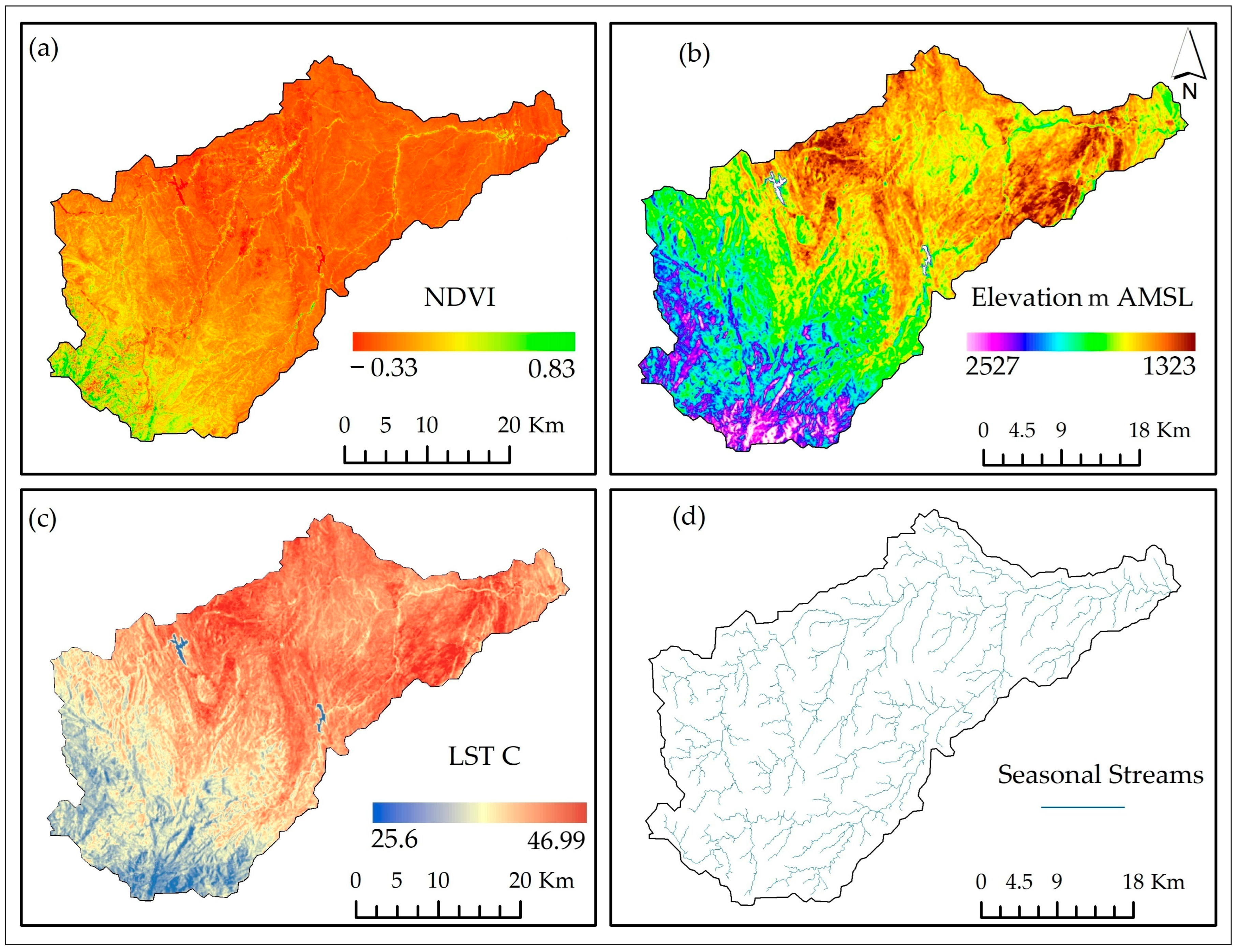
3.1. Vegetation Cover and Its Relationships with Altitude, LST, and Proximity to Streams

Figure 4 shows that higher elevations, predominantly in the southwestern region of the watershed, contribute to increased NDVI values due to cooler temperatures and higher moisture availability at higher altitudes. This elevation gradient supports vegetation by reducing thermal stress, as the land surface temperature (LST) decreases progressively from west to east. Similarly, the streamflow direction aligns with the elevation gradient, flowing west to east, facilitating water availability and sustaining vegetation health in downstream areas. This interconnected relationship highlights the influence of topography on vegetation, temperature, and hydrology.

The linear regression analysis revealed that the LST had the strongest linear relationship with the NDVI (R² = 0.42). Elevation was also a significant predictor (R² = 0.37). However, distance from streams exhibited a much weaker linear relationship, with an R² of only 0.007. While the linear regression model highlights significant relationships, it assumes a simplistic linear dependency, which may not fully capture complex ecological processes. To address this limitation, a generalized additive model (GAM) was applied to explore the nonlinear relationships between the NDVI and the predictors. Figure 5 presents the GAM results, where the smooth term for the LST was the strongest predictor (p < 2 × 10⁻¹⁶, edf = 10.23), explaining 50.44% of the variance in the NDVI. The elevation also exhibited a significant nonlinear relationship (p < 2 × 10⁻¹⁶, edf = 9.01), accounting for 40.96% of the NDVI variability. Conversely, distance from streams had a limited impact (p < 2 × 10⁻¹⁶, edf = 8.995), explaining only 4.28% of the variance. The GAM plot illustrates a steep decline in the NDVI near streams (within the first 500 m), beyond which the NDVI stabilizes. This indicates a localized influence of proximity to streams, which linear regression cannot effectively capture. The GAM approach, by incorporating flexibility in modeling nonlinear relationships, provides a more nuanced understanding of how the NDVI responds to environmental predictors across the study area.

The Shapiro–Wilk test revealed that the NDVI values for the highland and lower-elevation parts of the watershed deviated significantly from normality (p-values < 0.05). Consequently, the Wilcoxon rank-sum test was performed, which revealed a highly significant difference in the NDVI distributions between the groups (W = 5.401 × 10¹¹, p-value < 2.2 × 10⁻¹⁶). Elevation significantly impacts the NDVI.

3.2. Vegetation Cover in Relation to Slope Aspect

Table 2. Distribution area in square km. of the median NDVI during 2023 across different aspects in the watershed.

Aspect	Median NDVI During 2023								Total Area km2
	<0	0–0.05	0.05–0.1	0.1–0.15	0.15–0.2	0.2–0.25	0.25–0.3	>0.3
Flat	1.92	0.02	0.01	0.01	0.00	0.00	0.00	0.00	1.97
N	0.05	0.44	27.42	30.56	16.81	8.98	3.69	3.24	91.19
NE	0.19	1.08	68.70	73.27	35.56	16.53	6.50	5.65	207.48
E	0.15	1.50	79.98	83.76	35.05	15.17	5.69	6.24	227.53
SE	0.10	1.01	61.79	67.87	29.36	13.62	5.16	5.22	184.14
S	0.08	0.69	48.19	54.83	25.62	11.52	4.32	4.04	149.28
SW	0.21	0.74	48.45	50.75	24.13	10.73	4.16	4.34	143.50
W	0.16	0.70	55.22	55.14	26.97	14.07	7.15	7.30	166.72
NW	0.12	0.66	50.55	54.01	27.86	15.82	8.87	8.96	166.86
N	0.04	0.38	25.47	28.40	15.19	8.48	4.03	3.85	85.84
Total area km2	3.01	7.23	465.79	498.59	236.56	114.92	49.57	48.84	1424.52

shows the distribution of the NDVI in relation to slope aspects. The northeast and east aspects presented the highest NDVI values, reflecting better ecological conditions, whereas flat areas represented artificial lakes. This variation is influenced by the flow direction in the watershed, which is oriented from southwest to northeast.

Figure 6 presents the relationships between the aspect and vegetation distribution in the watershed. The east-facing (E) and northeast-facing (NE) slopes presented the highest vegetation cover, suggesting favorable conditions for vegetation growth. On the other hand, southern (S)- and southwestern (SW)-facing slopes exhibit lower cover. Flat areas are not shown in Figure 6 to maintain the correct orientation and represent the water bodies of Lake Al-Aqiq [36] and Wadi Tharad Dam Lake [37]. The findings highlight the significance of slope orientation in shaping vegetation patterns.

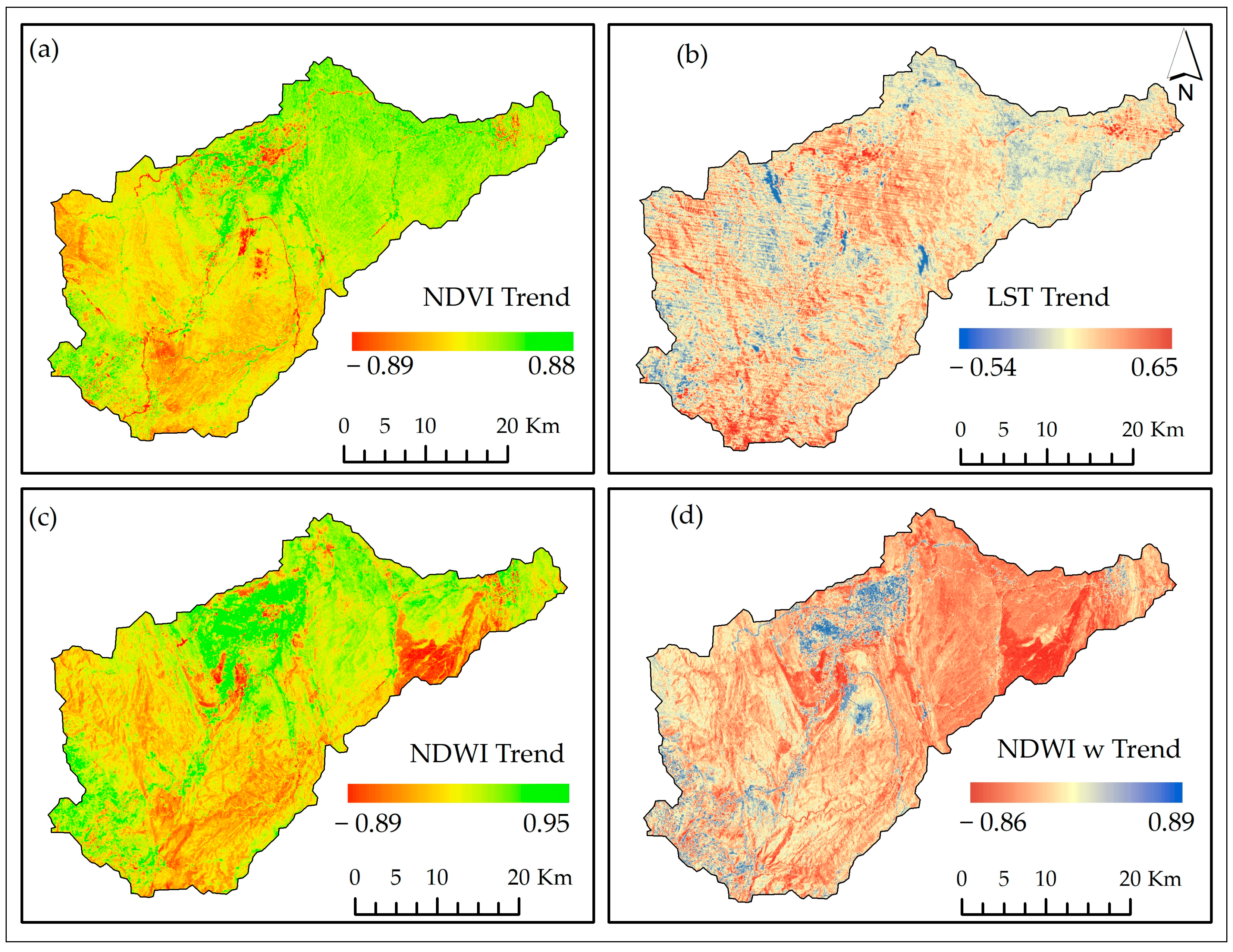
3.3. Spectral Indices Trends

Table 3. Mann–Kendall trend areas in square km. with significant trends from 1991–2023.

Indices	p < 0.05 (Above 95% CL)		p = 0.05–0.10 (90% < CL ≤ 95%)
	(−) Trend	(+) Trend	(−) Trend	(+) Trend
NDVI	91.66	184.71	37.28	77.94
LST	1.54	116.15	0.39	217.74
NDWI	138.51	456.97	36.47	72.20
NDWIw	804.92	93.51	88.33	11.54

summarizes the results of the Mann–Kendall trend analysis for the NDVI, LST, NDWI, and NDWI from 1991–2023, with a focus on statistically significant trends at the 90–100% confidence level. This figure highlights the extent of positive and negative trends in square kilometers.

Figure 7 provides a comprehensive visual representation of all trends in the spectral indices from 1991–2023, illustrating the spatial and temporal variations across the watershed.

The Shapiro–Wilk test results indicate that the NDVI trend for the highland and lower-elevation ecosystems deviated significantly from normality (p-values < 0.05). Consequently, the Wilcoxon rank-sum test was applied, revealing a highly significant difference in the NDVI trend distributions between the groups (W = 1.4235 × 10¹¹, p-value < 2.2 × 10⁻¹⁶). Elevation significantly influences the NDVI trends.

3.4. Ecological Stress Prediction Model

3.4.1. Model Performance and Significance of Smooth Terms in the GAM

Figure 8 shows the GAM results, illustrating the nonlinear relationships between the predictors and their effects on ecological stress. The GAM achieved an adjusted R-squared of 0.979. The smooth terms for all the predictors—Kendall’s τb coefficients of LST (s(LST)), NDWIw (s(NDWIw)), NDWI (s(NDWI)), and NDVI (s(NDVI)) were highly significant (p < 0.001), with effective degrees of freedom (edf) ranging from 7.9–8.9. High F statistics across predictors confirm their substantial contribution to the model. The low generalized cross-validation (GCV) score of 0.0077 underscores the model’s robustness and ability to capture complex nonlinear relationships in ecological stress dynamics (Figure 8).

3.4.2. Model Diagnostics and Cross-Validation

We applied a linear regression model to assess the relationship between the observed stress and the predicted stress. The model achieved a high R-squared value of 0.94. The F statistic (F = 1.173 × 10⁸, p < 2.2 × 10⁻¹⁶) underscores the model’s robustness. The coefficient for the predicted stress was 1.003 (p < 2 × 10⁻¹⁶), with a minimal intercept (−0.00298), reflecting near-perfect alignment between the observed and predicted values. A 10-fold cross-validation confirmed the model’s reliability, with the mean squared error (MSE) ranging from 0.0132–0.0134 and R-squared values ranging from 0.9865–0.9868.

3.4.3. Residual Diagnostics for Model Assessment

Residual diagnostics revealed minimal bias in predictions, with residuals ranging from −1.38 to 0.48 and a median close to zero. The standardized residuals fell largely within acceptable limits, with most values clustering around zero, confirming the model’s predictive accuracy and consistency. Minor outliers were observed but did not significantly affect model performance.

3.4.4. Spatial Validation of the GAM Model

The model’s spatial validation via Moran’s I revealed significant clustering (I = 0.21, z = 395.78, p < 0.0000001). The expected index (−0.000069) and near-zero variance indicate less than a 1% chance that the clustering is random.

The Shapiro–Wilk test revealed that the ecological stress for the highland and lower-elevation ecosystems deviated significantly from normality (p-values < 0.05). Consequently, the Wilcoxon rank-sum test was performed, indicating a highly significant difference in the ecological stress values between the groups (W = 3.2923 × 10¹², p-value < 2.2 × 10⁻¹⁶). Elevation strongly influences ecological stress.

3.5. Impact of Ecological Stress on Vegetation

The watershed is broadly divided into two elevation zones: high-altitude areas (1700–2383 m AMSL) and submontane or low-altitude areas (<1700 m AMSL) (see Figure 9). High-altitude zones experience severe ecological stress, particularly on southern and southwestern slopes, due to higher LSTs and declining NDVI trends. In contrast, low-altitude zones have reduced thermal stress. Aspect plays a crucial role in influencing vegetation distribution and stress levels through variations in thermal and water availability.

3.5.1. Ecological Stress in the Highlands Area (Above 1700 m AMSL)

Figure 10 shows that the ecological stress above 1700 m AMSL is marked by significant thermal stress and water scarcity, driven by elevated LST and declining NDWIw trends. The vegetation in these high-altitude areas presents varying stress levels that are significantly influenced by slope aspects. The northern and northeastern slopes face moderate stress with better water availability, whereas the southern and southwestern slopes endure severe stress, which is driven by higher temperatures and reduced vegetation productivity. Aspect strongly shapes species resilience and stress distribution.

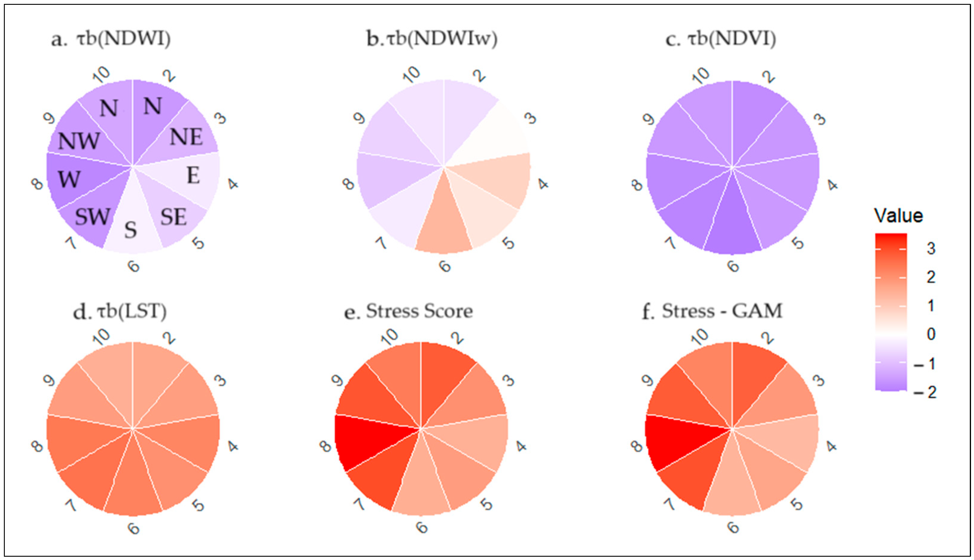
• Vegetation from 2015 to 2383 m AMSL: Figure 11 illustrates the trends in the ecological indices and stress levels across the different slope aspects. Woody plants are abundant on N and NE aspects, where declining NDVI trends (N: −1.77, NE: −1.60) suggest that plant health is under stress because increasing LST trends (N: +1.62, NE: +1.78) and declining NDWIw trends (N: −0.50) indicate thermal and water stress. Vegetation occurs sparsely on the E and SE aspects, with increasing LST (E: +2.18, SE: +2.02), and NDWI (E: +0.83, SE: +0.48), but decreasing NDVI (E: −1.58, SE: −1.57) trends. South-facing (S) slopes presented the highest stress levels for most vegetation, due to higher LST trends (S: 2.26) and deteriorating NDVI trends (S: −2.02). The vegetation on the W and SW slopes faces severe ecological stress due to high LST (W: 2.39, SW: 2.49) and declining NDWIw (W: −0.87, SW: −0.31) trends.
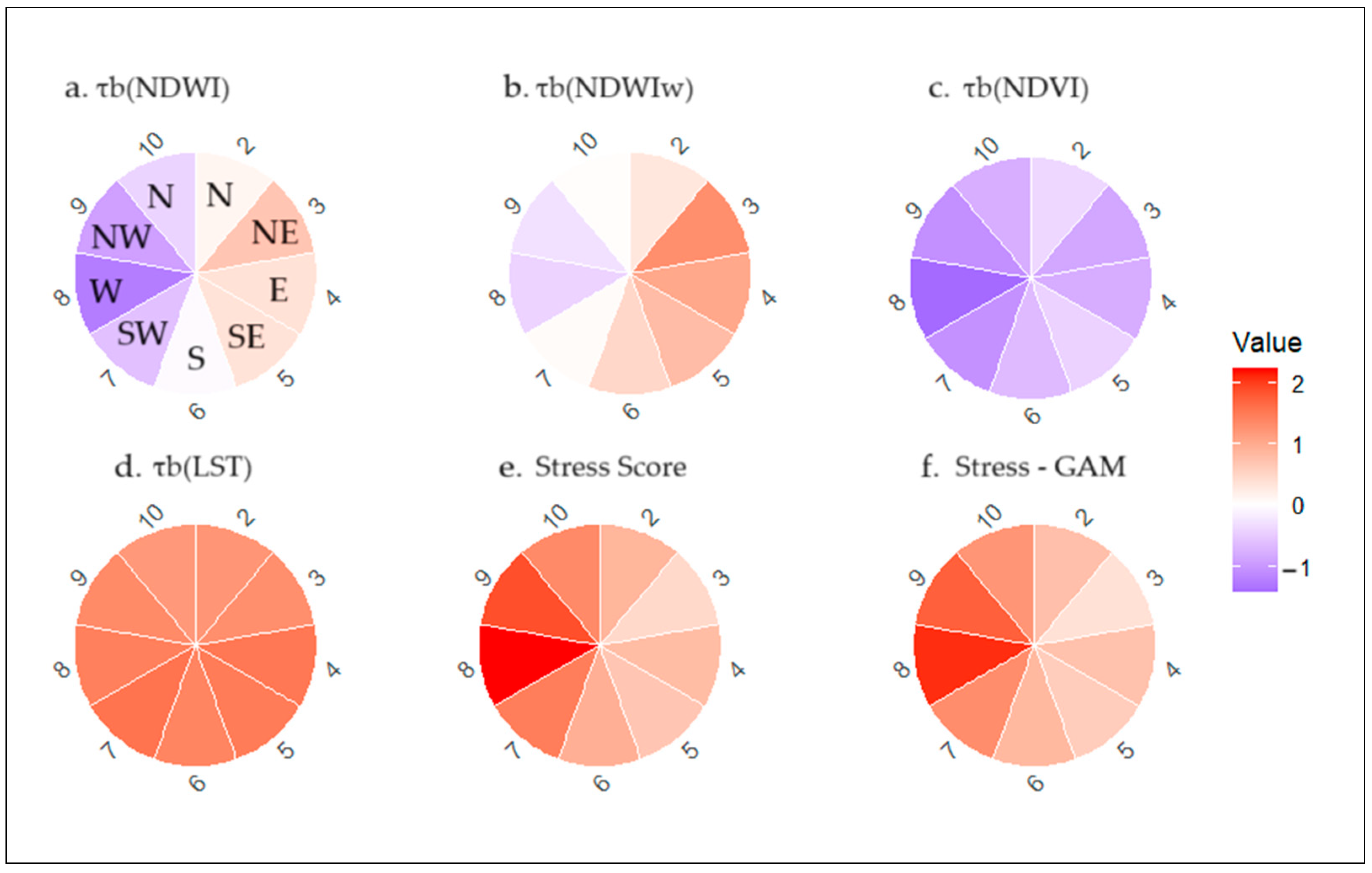
• Vegetation at 1900–2085 m AMSL: Figure 12 illustrates the trends in ecological indices and stress levels across the different slope aspects. Vegetation is more prevalent on the NW and SW aspects, where moderately increasing LSTs (NW: 1.32, SW: 1.55) are accompanied by high ecological stress, as indicated by sharp declines in the NDVI (NW: −1.08, SW: −1.06). For NW aspects, significant decreases in the NDWI trends (−0.93) and NDWIw trends (−0.29) reflect changes in both the vegetation water content and surface water/moisture stress. Vegetation occurs sparsely, with a preference for S aspects, where a moderate increase in LST trends (1.39) and slightly increasing NDWIw trends (0.47) suggest reduced thermal stress but limited improvement in vegetation health (NDVI trend: −0.66). Shrubs on SW and W aspects, facing severe stress due to increased LST trends (SW: 1.55, W: 1.43) and decreased water availability (NDWIw trend: SW: +0.05, W: −0.42). Herbs are abundant across multiple aspects but show better resilience in terms of S aspects due to moderate LST trends and higher NDWIw trends, despite decreasing productivity (NDVI trend: −0.66).
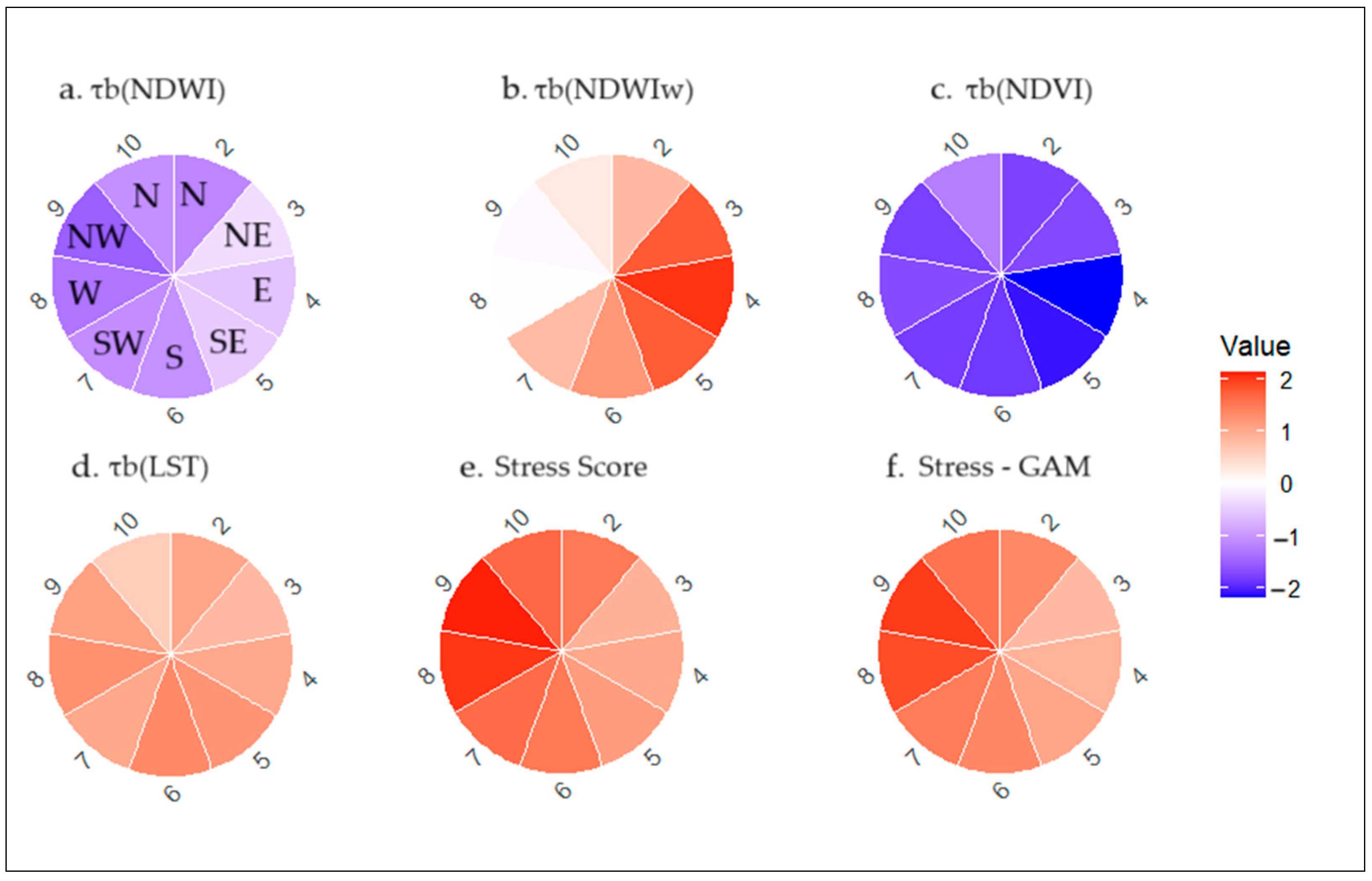
• Vegetation at 1700–2085 m AMSL: Figure 13 illustrates the trends in the ecological indices and stress levels across different slope aspects. Trees occur predominantly on the S and SE aspects, where moderate LST trends (S: +1.32, SE: +1.21) and increasing NDWIw trends (S: +1.18, SE: +1.75) are offset by declining NDVI trends (S: −1.85, SE: −2.10), indicating deteriorating vegetation health. Vegetation is present across various aspects, and demonstrates resilience on SE and NE slopes, where higher NDWIw trends (NE: +1.77, SE: +1.75) support better water availability, despite significant declines in vegetation productivity (NDVI trends: NE: −1.72, SE: −2.10). With respect to the W and NW aspects, there was ecological stress due to high LST trends (W: +1.25, NW: +1.08) and declining water availability (NDWIw trends: W: −0.02, NW: −0.07). Shrubs are abundant on SE slopes and benefit from moderate water retention (NDWIw trend: +1.75). However, herbaceous species exhibit better health on NE slopes, where thermal stress is lowest (LST trend: 0.81).

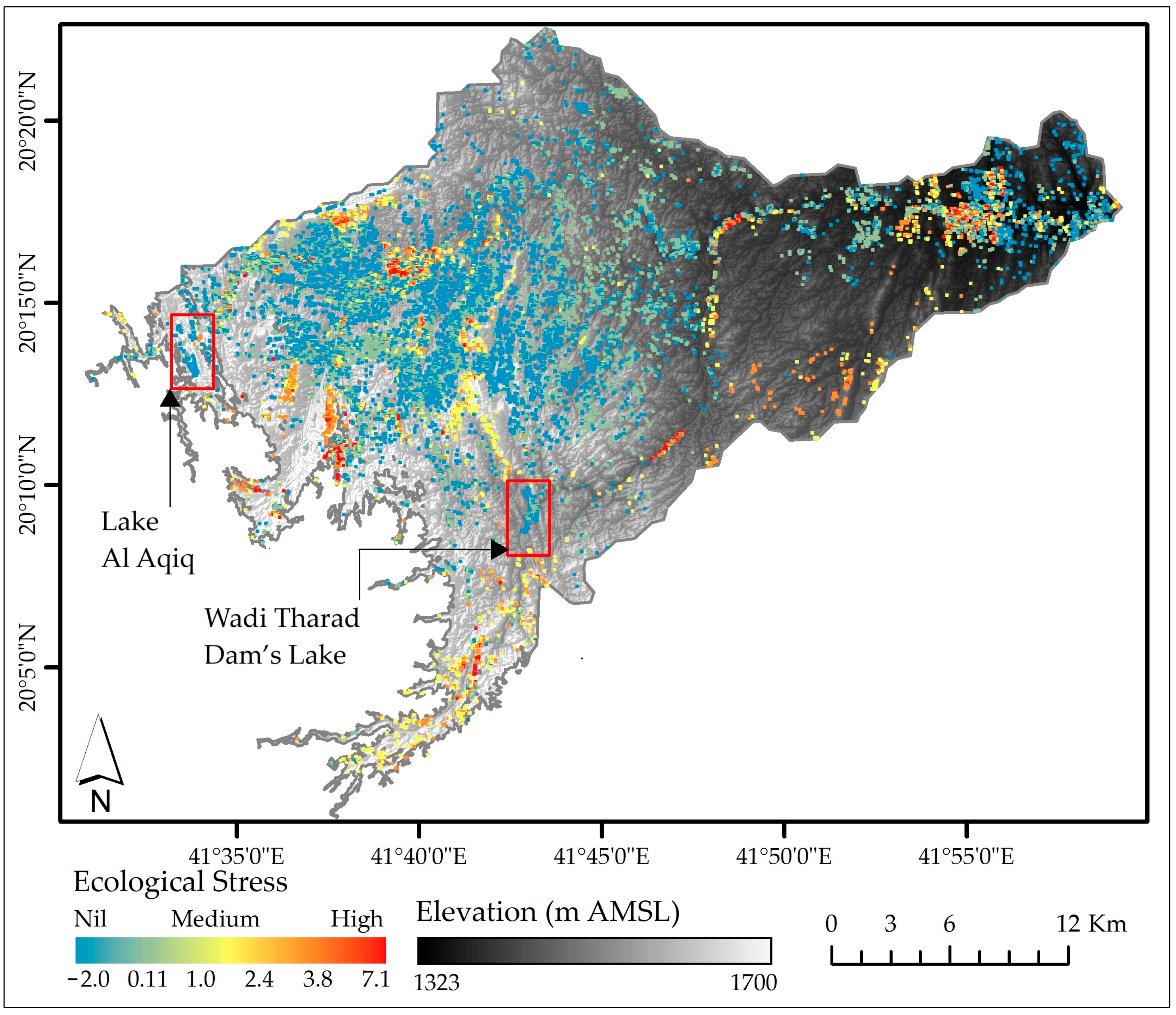
3.5.2. Ecological Stress in the Lower Part of the Watershed (Below 1700 m AMSL)

Figure 14 illustrates the ecological stress below 1700 m AMSL, which is influenced by moderate thermal and water stress. Flat terrains, especially those near artificial lakes, exhibit reduced thermal stress but declining NDVI trends, whereas sloped terrains show aspect-driven variations, with southeastern and southern slopes facing relatively high stress levels.

Figure 15 illustrates the trends in the ecological indices and stress levels across the different slope aspects. The flat aspect is associated with lakes having the lowest thermal stress due to changes in land cover to artificial lakes, with a significant negative LST trend (−8.59), and the highest water availability, indicated by a strong positive NDWIw trend (2.42). However, despite favorable water conditions, vegetation health is highly stressed, as indicated by a declining NDVI trend (−2.73), suggesting reduced productivity, potentially due to changes in land cover to artificial lakes.

On sloped terrains, vegetation is prominent in the SE and S aspects, where moderate LST trends (SE: 1.22, S: 1.25) and declining NDWI trends (SE: 0.11, S: −0.03) indicate moderate thermal and water stress. Similarly, woody plants are found on the E and NE aspects, benefiting from slightly lower stress levels (LST trends: E: 1.21, NE: 1.19) and moderate water availability (NDWIw trends: E: 0.16, NE: 0.18).

4. Discussion

This study integrates multitemporal Landsat SR-derived spectral indices with the Copernicus DEM to assess 2023 vegetation cover, spectral index trends from 1991–2023, ecological stress modeling, and the impact of ecological stress on major plant species within the watersheds of the Al-Baha Highlands, Saudi Arabia. The following sections discuss the adopted methods and findings.

4.1. Vegetation Cover and Its Relationship with Land Surface Temperature, Proximity to Streams, Altitude, and Slope Aspect

The results revealed that the NDVI significantly differed between highlands (1700–2557 m) and lower-elevation areas (<1700 m). Highlands have higher and more varying NDVI, indicating denser vegetation and diverse ecological conditions, whereas lower elevations have lower NDVI, suggesting limited vegetation. This phenomenon can be attributed to several interrelated factors. Elevated areas typically receive more rainfall than lower regions do, providing essential moisture that supports plant growth. This pattern has been observed in the Asir Mountains of Saudi Arabia, where higher altitudes experience greater precipitation, leading to richer vegetation [38]. Higher elevations generally have cooler temperatures, which can reduce evapotranspiration rates and water stress in plants. This creates a more favorable environment for diverse plant species to thrive, as observed in various mountainous regions [39]. The combination of increased moisture and organic matter from vegetation at relatively high altitudes enhances soil fertility and structure, promoting further plant growth. Studies in mountain ecosystems have shown that soil properties improve with elevation, supporting more diverse plant communities [40]. The localized influence of proximity to streams is also interesting; streams often deposit sediments during flow events, enriching adjacent soils with nutrients. This process creates fertile conditions that promote diverse plant communities [41]. The areas near streams experience moderate temperatures and increased humidity. These microclimatic conditions reduce plant stress and facilitate the growth of various species [42]. Plants near streams have better access to groundwater, which is vital during dry periods. This ability enables them to maintain physiological processes and sustain growth even under drought conditions.

Aspect analysis provided additional ecological insights, with east- and northeast-facing slopes exhibiting greater vegetation cover due to optimal solar radiation and moisture supply. These findings agree with those of Schaefer et al. (2024), who emphasized the role of such aspects in shaping microclimates [43].

4.2. Trends of Vegetation and Environmental Variables

This study effectively captured long-term patterns in the NDVI, NDWI, NDWIw, and LST. The dominance of positive NDVI trends (184.71 km², p < 0.05) indicates improved vegetation health in certain areas, which aligns with the global greening patterns observed in semiarid ecosystems [44]. However, the coexistence of negative trends (91.66 km²) highlights vegetation degradation, which is likely linked to anthropogenic pressures and climatic variability, to relate the NDVI trend with anthropogenic pressure. The relationship between the NDVI trend and distance from roads was modeled via an exponential function: NDVI trend = a⋅e^{−b⋅Distance}. The results revealed a negative NDVI trend near roads, which transitioned to positive values as distance increased. Both parameters, a = −0.9017 and b = 0.0221, were highly significant (p < 0.001), supporting the idea of anthropogenic pressures on vegetation. The model was fitted via nonlinear regression, which captured the nonlinear pattern of the NDVI trend with increasing distance. However, Figure 16 illustrates that the negative NDVI trend is more strongly associated with highways; on the other hand, residential and other roads show positive trends along the roads.

The pronounced positive trends in vegetation water content (NDWI) (456.97 km², p < 0.05) suggest enhanced water availability, possibly due to effective water management practices in certain areas. However, the stark negative trends in NDWIw (804.92 km²) reveal significant degradation, reflecting the challenges of hydrological stress, over-extraction, or altered land use.

LST trends further underscore widespread warming, with positive trends dominating (116.15 km², p < 0.05). This aligns with global trends of increasing surface temperatures in mountainous regions [43,44,45], which exacerbate evapotranspiration rates and reduce water availability for vegetation. The near absence of negative LST trends (1.54 km²) reinforces the idea of persistent warming across the study area, a critical driver of ecological stress. The significant differences in the NDVI trends between the highland and lower-elevation ecosystems (see Figure 16), as revealed by the Wilcoxon rank-sum test, also emphasize the role of increased LSTs in modulating vegetation responses.

4.3. Ecological Stress Model

The ecological stress model developed in this study integrates trends from the NDVI, LST, NDWI, and NDWIw via a generalized additive model (GAM). This nonlinear modeling approach is particularly suited for capturing the complexity of environmental variables and their interactions. The model’s robustness, demonstrated by a high adjusted R² (0.979) and low GCV score (0.0077), underscores its reliability. Compared with linear models commonly used in similar studies, the GAM provides greater flexibility and precision in capturing nonlinear relationships, which are crucial in heterogeneous landscapes such as Saudi Arabia’s highlands.

The method of applying p-value masking (p < 0.1) ensures the statistical reliability of the trends incorporated into the stress score. This approach aligns with previous studies on ecological stress modeling, such as those by Wang et al. (2016), which emphasize the importance of filtering nonsignificant trends to improve model performance [46]. However, one limitation of this study is the lack of temporal seasonality analysis, which could provide deeper insights into intra-annual variations in ecological stress. Additionally, while the GAM effectively models continuous predictors, the impact of abrupt land-use changes may be underrepresented.

Species-specific responses to stress further underscore the importance of integrating biological data with ecological modeling. The vulnerability of high-altitude species such as Juniperus procera to thermal and water stress highlights the compound effects of climatic and topographic variables, as observed in other montane regions (Ali et al., 2018) [47]. Conversely, the resilience of lower-elevation species such as Rhazya stricta in flat terrains with lakes demonstrates the potential of water management to mitigate stress, which is consistent with findings on adaptive strategies in similar ecological zones [48].

Despite the model’s strong performance, limitations exist. The stress scoring system relies on predefined weights, which, while scientifically grounded, may oversimplify complex ecological interactions. Moreover, the analysis focused on static species distributions, potentially overlooking phenological changes or interspecies competition. Future studies could benefit from integrating temporal dynamics and expanding the variable set to include soil properties and anthropogenic factors, as suggested by Huang et al. (2017) [49].

This research contributes significantly to the field of ecological modeling by providing a detailed spatial and species-level assessment of stress in a climatically vulnerable region. The application of advanced statistical and spatial techniques offers a scalable framework for ecological stress prediction, with implications for conservation planning and climate adaptation strategies.

4.4. Implications and Future Directions

The findings of this study have significant implications for sustainable ecosystem management in hilly regions. The identification of high-stress zones, particularly those on south-facing slopes and low-altitude areas, can inform reforestation and water management strategies.

Future studies should integrate finer spatial and temporal resolution data to capture seasonal variations in stress and its impact on vegetation. The incorporation of additional anthropogenic factors, such as grazing and urban expansion, would provide a more comprehensive picture of ecological dynamics. Furthermore, coupling this model with remote sensing techniques such as hyperspectral imaging could increase its ability to detect subtle changes in vegetation health and stress. This study provides a scientifically rigorous framework for understanding and managing ecological stress in Saudi Arabia’s unique environment. Linking environmental trends to species-level impacts offers critical insights for preserving biodiversity and ensuring the sustainability of fragile ecosystems.

5. Conclusions

This study provides a comprehensive assessment of the ecological stress in the Al-Baha Highlands, integrating trends in vegetation and environmental variables to model their impacts on vegetation. By leveraging multi-temporal Landsat surface reflectance (SR) products and the Copernicus DEM, this research links spatial and temporal variations in the NDVI, LST, NDWI, and NDWIw with ecological stress dynamics. The analysis highlights the critical role of elevation, aspect, and proximity to streams in shaping vegetation distribution in hilly environments. The use of a generalized additive model (GAM) framework enabled the identification of nonlinear relationships between environmental predictors and stress scores, achieving high predictive accuracy. This approach, combined with robust statistical validation, underscores the importance of integrating multiple environmental variables to develop holistic stress models. High-altitude areas (>1700 m AMSL) experience pronounced thermal and water stress, particularly on southern and southwestern slopes, where elevated LSTs and declining NDWI trends significantly reduce vegetation, impacting species such as Juniperus procera. In contrast, the northern and northeastern slopes exhibit moderate stress. Aspect is not a direct driver of vegetation stress levels and patterns; however, it significantly influences environmental conditions, such as solar radiation, moisture availability, and wind exposure. Consequently, vegetation stress can be analyzed in relation to aspects, particularly because of differences between windward and leeward slopes, which affect microclimatic conditions and exposure to climatic stressors. Findings on aspect-driven vegetation stress variations can help policymakers in designing targeted afforestation and land restoration strategies. Future research should incorporate temporal seasonality, anthropogenic influences, and advanced remote sensing techniques to enhance ecological stress modeling. By identifying high-risk zones and species-specific vulnerabilities, this study provides actionable recommendations for reforestation, water resource management, and conservation planning in fragile ecosystems, contributing to the preservation of biodiversity and ecological sustainability in hilly environments.

References

1. Hollenbeck, E.C.; Sax, D.F. Experimental evidence of climate change extinction risk in Neotropical montane epiphytes. Nat. Commun. 2024, 15, 6045. [Google Scholar] [CrossRef] [PubMed]
2. Telwala, Y.; Brook, B.W.; Manish, K.; Pandit, M.K. Climate-Induced Elevational Range Shifts and Increase in Plant Species Richness in a Himalayan Biodiversity Epicenter. PLoS ONE 2013, 8, e57103. [Google Scholar] [CrossRef]
3. Hassan, T.; Gulzar, R.; Hamid, M.; Ahmad, R.; Waza, S.A.; Khuroo, A.A. Plant Phenology Shifts under Climate Warming: A Systematic Review of Recent Scientific Literature. Environ. Monit. Assess. 2023, 196, 36. [Google Scholar] [CrossRef]
4. Thomas, J.; El-Sheikh, M.A.; Alatar, A.A. Endemics and Endangered Species in the Biodiversity Hotspot of the Shada Mountains, Saudi Arabia. J. Arid Land 2016, 9, 109–121. [Google Scholar] [CrossRef]
5. Al-Aklabi, A.; Al-Khulaidi, A.W.; Hussain, A.; Al-Sagheer, N. Main Vegetation Types and Plant Species Diversity along an Altitudinal Gradient of Al Baha Region, Saudi Arabia. Saudi J. Biol. Sci. 2016, 23, 687–697. [Google Scholar] [CrossRef]
6. Ghazanfar, S.A.; Fisher, M. Vegetation of the Arabian Peninsula; Springer: Berlin/Heidelberg, Germany, 2014. [Google Scholar] [CrossRef]
7. Ibrahim, H.M.; Alghamdi, A.G.; Aly, A.A. Assessing Drought Patterns in Al-Baha: Implications for Water Resources and Climate Adaptation. Sustainability 2024, 16, 9882. [Google Scholar] [CrossRef]
8. Almazroui, M. Changes in Temperature Trends and Extremes over Saudi Arabia for the Period 1978–2019. Adv. Meteorol. 2020, 2020, 1–21. [Google Scholar] [CrossRef]
9. El-Rawy, M.; Batelaan, O.; Al-Arifi, N.; Alotaibi, A.; Abdalla, F.; Gabr, M.E. Climate Change Impacts on Water Resources in Arid and Semi-Arid Regions: A Case Study in Saudi Arabia. Water 2023, 15, 606. [Google Scholar] [CrossRef]
10. Pellikka, P.K.E.; Al Shaikh, A.Y.; Maeda, E.; Adhikari, H. Land Cover Changes in Montane Cloud Forests in Kenya and Its Potential Impacts on Water Availability—Similarity in Saudi Arabia. In Proceedings of the 6th International Conference on Water Resources and Arid Environments (ICWRAE 6), Riyadh, Saudi Arabia, 16–17 December 2014; Volume 6. [Google Scholar]
11. Sui, X.; Xu, Q.; Tao, H.; Zhu, B.; Li, G.; Zhang, Z. Vegetation Dynamics and Recovery Potential in Arid and Semi-Arid Northwest China. Plants 2024, 13, 3412. [Google Scholar] [CrossRef]
12. Zhao, Y.; Hu, C.; Dong, X.; Li, J. NDVI Characteristics and Influencing Factors of Typical Ecosystems in the Semi-Arid Region of Northern China: A Case Study of the Hulunbuir Grassland. Land 2023, 12, 713. [Google Scholar] [CrossRef]
13. Chang, S.; Chen, H.; Wu, B.; Nasanbat, E.; Yan, N.; Davdai, B. A Practical Satellite-Derived Vegetation Drought Index for Arid and Semi-Arid Grassland Drought Monitoring. Remote Sens. 2021, 13, 414. [Google Scholar] [CrossRef]
14. Serrano, J.; Shahidian, S.; Marques da Silva, J. Evaluation of Normalized Difference Water Index as a Tool for Monitoring Pasture Seasonal and Inter-Annual Variability in a Mediterranean Agro-Silvo-Pastoral System. Water 2019, 11, 62. [Google Scholar] [CrossRef]
15. Reiners, P.; Sobrino, J.; Kuenzer, C. Satellite-Derived Land Surface Temperature Dynamics in the Context of Global Change—A Review. Remote Sens. 2023, 15, 1857. [Google Scholar] [CrossRef]
16. Martins Gnecco, V.; Pigliautile, I.; Pisello, A.L. Long-Term Thermal Comfort Monitoring via Wearable Sensing Techniques: Correlation between Environmental Metrics and Subjective Perception. Sensors 2023, 23, 576. [Google Scholar] [CrossRef] [PubMed]
17. Akhundzadah, N.A. Analyzing Temperature, Precipitation, and River Discharge Trends in Afghanistan’s Main River Basins Using Innovative Trend Analysis, Mann–Kendall, and Sen’s Slope Methods. Climate 2024, 12, 196. [Google Scholar] [CrossRef]
18. Al-Huqail, A.A.; Islam, Z.; Al-Harbi, H.F. An ML-Based Ensemble Approach for the Precision Classification of Mangroves, Trend Analysis, and Priority Reforestation Areas in Asir, Saudi Arabia. Sustainability 2024, 16, 10355. [Google Scholar] [CrossRef]
19. Pesaresi, S.; Mancini, A.; Quattrini, G.; Casavecchia, S. Evaluation and Selection of Multi-Spectral Indices to Classify Vegetation Using Multivariate Functional Principal Component Analysis. Remote Sens. 2024, 16, 1224. [Google Scholar] [CrossRef]
20. Al-Mutairi, M.; Labban, A.; Abdeldym, A.; Abdel Basset, H. Trend Analysis and Fluctuations of Winter Temperature over Saudi Arabia. Climate 2023, 11, 67. [Google Scholar] [CrossRef]
21. K C, M.; Leigh, L.; Pinto, C.T.; Kaewmanee, M. Method of Validating Satellite Surface Reflectance Product Using Empirical Line Method. Remote Sens. 2023, 15, 2240. [Google Scholar] [CrossRef]
22. Potapov, P.; Hansen, M.C.; Kommareddy, I.; Kommareddy, A.; Turubanova, S.; Pickens, A.; Adusei, B.; Tyukavina, A.; Ying, Q. Landsat Analysis Ready Data for Global Land Cover and Land Cover Change Mapping. Remote Sens. 2020, 12, 426. [Google Scholar] [CrossRef]
23. Franks, S.; Rengarajan, R. Evaluation of Copernicus DEM and Comparison to the DEM Used for Landsat Collection-2 Processing. Remote Sens. 2023, 15, 2509. [Google Scholar] [CrossRef]
24. Marešová, J.; Gdulová, K.; Pracná, P.; Moravec, D.; Gábor, L.; Prošek, J.; Barták, V.; Moudrý, V. Applicability of Data Acquisition Characteristics to the Identification of Local Artifacts in Global Digital Elevation Models: Comparison of the Copernicus and TanDEM-X DEMs. Remote Sens. 2021, 13, 3931. [Google Scholar] [CrossRef]
25. Robinson, N.P.; Allred, B.W.; Jones, M.O.; Moreno, A.; Kimball, J.S.; Naugle, D.E.; Erickson, T.A.; Richardson, A.D. A Dynamic Landsat Derived Normalized Difference Vegetation Index (NDVI) Product for the Conterminous United States. Remote Sens. 2017, 9, 863. [Google Scholar] [CrossRef]
26. Laonamsai, J.; Julphunthong, P.; Saprathet, T.; Kimmany, B.; Ganchanasuragit, T.; Chomcheawchan, P.; Tomun, N. Utilizing NDWI, MNDWI, SAVI, WRI, and AWEI for Estimating Erosion and Deposition in Ping River in Thailand. Hydrology 2023, 10, 70. [Google Scholar] [CrossRef]
27. Chen, J.; Wang, Y.; Wang, J.; Zhang, Y.; Xu, Y.; Yang, O.; Zhang, R.; Wang, J.; Wang, Z.; Lu, F.; et al. The Performance of Landsat-8 and Landsat-9 Data for Water Body Extraction Based on Various Water Indices: A Comparative Analysis. Remote Sens. 2024, 16, 1984. [Google Scholar] [CrossRef]
28. Wang, L.; Lu, Y.; Yao, Y. Comparison of Three Algorithms for the Retrieval of Land Surface Temperature from Landsat 8 Images. Sensors 2019, 19, 5049. [Google Scholar] [CrossRef]
29. Miao, X.; Zhang, Y.; Zhang, J.; Zhou, X. Temperature and Emissivity Smoothing Separation with Nonlinear Relation of Brightness Temperature and Emissivity for Thermal Infrared Sensors. Remote Sens. 2019, 11, 2959. [Google Scholar] [CrossRef]
30. Sen, P.K. Estimates of the Regression Coefficient Based on Kendall’s Tau. J. Am. Stat. Assoc. 1968, 63, 1379–1389. [Google Scholar] [CrossRef]
31. Wang, F.; Shao, W.; Yu, H.; Kan, G.; He, X.; Zhang, D.; Ren, M.; Wang, G. Re-Evaluation of the Power of the Mann–Kendall Test for Detecting Monotonic Trends in Hydrometeorological Time Series. Front. Earth Sci. 2020, 8, 14. [Google Scholar] [CrossRef]
32. Liu, L.; Li, A.; Zhu, L.; Xue, S.; Li, J.; Zhang, C.; Yu, W.; Ma, Z.; Zhuang, H.; Jiang, Z.; et al. The Application of the Generalized Additive Model to Represent Macrobenthos near Xiaoqing Estuary, Laizhou Bay. Biology 2023, 12, 1146. [Google Scholar] [CrossRef]
33. Zhang, X.; Yang, F.; Zhang, J.; Dai, Q. Using GAMs to Explore the Influence Factors and Their Interactions on Land Surface Temperature: A Case Study in Nanjing. Land 2024, 13, 465. [Google Scholar] [CrossRef]
34. White, J.; Power, S.D. k-Fold Cross-Validation Can Significantly Over-Estimate True Classification Accuracy in Common EEG-Based Passive BCI Experimental Designs: An Empirical Investigation. Sensors 2023, 23, 6077. [Google Scholar] [CrossRef] [PubMed]
35. Sun, S.; Zhang, H. Flow-Data-Based Global Spatial Autocorrelation Measurements for Evaluating Spatial Interactions. ISPRS Int. J. Geo. Inf. 2023, 12, 396. [Google Scholar] [CrossRef]
36. Alghamdi, B.A.; El Mannoubi, I.; Zabin, S.A. Heavy Metals Contamination in Sediments of Wadi Al-Aqiq Water Reservoir Dam at Al-Baha Region, KSA: Their Identification and Assessment. Hum. Ecol. Risk Assess. 2019, 25, 618–631. [Google Scholar] [CrossRef]
37. Wadi Tharad. Available online: https://aldalila.moc.gov.sa/en/route-detail/08b84370-dd96-11ec-aa01-1d7ac881c19e/grid (accessed on 24 February 2025).
38. Ghazal, A.F. Vegetation Patterns and Plant Communities’ Distribution along an Altitudinal Gradient at Asir Mountain, Southwest Saudi Arabia. Pak. J. Bot. 2015, 47, 1377–1389. [Google Scholar]
39. He, X.; Yin, F.; Arif, M.; Zheng, J.; Chen, Y.; Geng, Q.; Ni, X.; Li, C. Diversity Patterns of Plant Communities along an Elevational Gradient in Arid and Semi-Arid Mountain Ecosystems in China. Plants 2024, 13, 2858. [Google Scholar] [CrossRef]
40. Abd El-Ghani, M.; Borki, A. How Elevation and Soil Properties Affect Plant Distribution Patterns and Species Diversity in the Mediterranean Mountain Ecosystem of Al-Jabal Al-Akhdar, Libya. J. Mt. Sci. 2024, 21, 3683–3701. [Google Scholar] [CrossRef]
41. Sehati, M.T.; Nohegar, A.; Esmailpour, Y.; Gholami, H. The Role of Geometric Properties of Ephemeral Arid Streams in the Control of Soil and Sediment Quality, and Vegetation Canopy Distribution: A Case Study in the Southwest of Fars Province, Iran. J. Soils Sediments 2023, 23, 1789–1805. [Google Scholar] [CrossRef]
42. Julian, J.P. Riparian Vegetation as an Indicator of Stream Channel Presence and Connectivity in Arid Environments. Available online: https://nicholasinstitute.duke.edu/publications/riparian-vegetation-indicator-stream-channel-presence-and-cconnectivity-arid (accessed on 13 December 2024).
43. Schaefer, M.L.; Bogacki, W.; Lopez Caceres, M.L.; Kirschbauer, L.; Kato, C.; Kikuchi, S.-I. Influence of Slope Aspect and Vegetation on the Soil Moisture Response to Snowmelt in the German Alps. Hydrology 2024, 11, 101. [Google Scholar] [CrossRef]
44. Wu, Z.; Bi, J.; Gao, Y. Drivers and Environmental Impacts of Vegetation Greening in a Semi-Arid Region of Northwest China since 2000. Remote Sens. 2021, 13, 4246. [Google Scholar] [CrossRef]
45. Wang, S.; Aihaiti, A.; Mamtimin, A.; Sayit, H.; Peng, J.; Liu, Y.; Wang, Y.; Gao, J.; Song, M.; Wen, C.; et al. Increases in Temperature and Precipitation in the Different Regions of the Tarim River Basin Between 1961 and 2021 Show Spatial and Temporal Heterogeneity. Remote Sens. 2024, 16, 4612. [Google Scholar] [CrossRef]
46. Wang, J.; Rich, P.M.; Price, K.P. Temporal Responses of NDVI to Precipitation and Temperature in the Central Great Plains, USA. Int. J. Remote Sens. 2016, 27, 865–874. [Google Scholar] [CrossRef]
47. Ali, M.; Rahman, K.U.; Ullah, H.; Shang, S.; Mao, D.; Han, M. Land Reforestation and Its Impact on the Environmental Footprints Across Districts of Khyber Pakhtunkhwa in Pakistan. Water 2024, 16, 3009. [Google Scholar] [CrossRef]
48. Davidson, A. Adaptive Strategies of Desert Flora: Water Management and Resilience in Arid Ecosystems. Ecol. Appl. 2014, 24, 1363–1377. [Google Scholar] [CrossRef]
49. Huang, J.; Yu, H.; Dai, A.; Wei, Y.; Kang, L. Drylands Face Potential Threats under Climate Change Scenarios. Nat. Clim. Change 2017, 7, 417–422. [Google Scholar] [CrossRef]
Figure 1. (a) Location of Al-Baha in Saudi Arabia. (b) Watersheds within Al-Baha Province; watershed boundary in red indicates the area of interest. (c) Altitude range in the watershed of interest; white line indicates the 1700 m contour.
Sustainability 17 02854 g001
Figure 2. Subfigures (ai) show trends in the annual average of key climatic variables in the watershed from 1991–2023, sourced from TerraClimate and analyzed using interquartile ranges.
Sustainability 17 02854 g002
Figure 3. Framework of the method for spectral indices, trend analysis, and ecological stress and its impact on major species via Landsat TM, ETM+, OLI/TIRS sensor, and Copernicus DEM GLO-30 satellite data, arrow symbols show variables relationship.
Sustainability 17 02854 g003
Figure 4. Spatial patterns of the ecological variables in the study area: subfigures (a) median NDVI (2023) illustrating vegetation distribution, (b) elevation (AMSL) showing topographic variation, (c) median LST (2023) in Celsius, and (d) seasonal stream.
Sustainability 17 02854 g004
Figure 5. GAM-derived relationships between the NDVI and predictors. Subfigure (a): significant nonlinear relationship with elevation, accounting for 40.96% of the NDVI variability. (b) LST: strongest predictor, explaining 50.44% of the variance in the NDVI. (c) Distance from streams: localized influence near streams, explaining 4.28% of the variability.
Sustainability 17 02854 g005
Figure 6. Distribution of the NDVI across different aspects within the watershed. Directional labels: N (North), NE (Northeast), E (East), SE (Southeast), S (South), SW (Southwest), W (West), NW (Northwest).
Sustainability 17 02854 g006
Figure 7. Spectral index trends with p-values < 1 (which shows all trends) based on Kendall’s tau-b correlation (1991–2023) for the Al-Baha Highlands. The subfigures (ad) represent trends for the NDVI, LST, NDWI, and NDWIw, respectively.
Sustainability 17 02854 g007
Figure 8. Response curves of the predictors for predicting ecological stress via generalized additive model (GAM) analysis.
Sustainability 17 02854 g008
Figure 9. Predicted ecological stress calculated via the spectral indices Kendall’s τb (p < 0.1) for the input variables at the watershed level in the Al-Baha Highlands, as modeled via a GAM.
Sustainability 17 02854 g009
Figure 10. Predicted ecological stress above 1700 m calculated via the spectral indices Kendall’s τb (p < 0.1) across the elevation zones: subfigures (a) 2015–2383 m AMSL, (b) 1900–2085 m AMSL, (c) 1700–2085 m AMSL, and (d) 1700–1810 m AMSL. Red-boxed areas highlight regions with significant ecological stress. These areas were further analyzed in relation to aspect and dominant plant species.
Sustainability 17 02854 g010
Figure 11. Aspect-wise trends in (a) NDWI, (b) NDWIw, (c) NDVI, (d) LST, (e) stress score, and (f) GAM-predicted stress across elevations ranging from 2015 to 2383 m AMSL. Red shading indicates positive trends, whereas blue shading indicates negative trends from 1991–2023.
Sustainability 17 02854 g011
Figure 12. Aspect-wise trends in (a) NDWI, (b) NDWIw, (c) NDVI, (d) LST, (e) stress score, and (f) GAM-predicted stress across elevations ranging from 1900–2085 m AMSL. Red shading indicates positive trends, whereas blue shading indicates negative trends from 1991–2023.
Sustainability 17 02854 g012
Figure 13. Aspect-wise trends in (a) NDWI, (b) NDWIw, (c) NDVI, (d) LST, (e) stress score, and (f) GAM-predicted stress across elevations ranging from 1700 m to 2085 m AMSL. Red shading indicates positive trends, whereas blue shading indicates negative trends from 1991–2023.
Sustainability 17 02854 g013
Figure 14. Ecological stress in the watershed from 1323 m to 1700 m AMSL.
Sustainability 17 02854 g014
Figure 15. Aspect-wise trends in (a) NDWI, (b) NDWIw, (c) NDVI, (d) LST, (e) stress score, and (f) GAM-predicted stress across elevations ranging from 1323 m to 1700 m AMSL. Red shading indicates positive trends, whereas blue shading indicates negative trends from 1991–2023.
Sustainability 17 02854 g015
Figure 16. NDVI trends (1991–2023) categorized by elevation zones (>1700 m AMSL and <1700 m AMSL) and proximity to roads as a proxy for anthropogenic influence. Red areas represent negative NDVI trends (up to −0.9), and green areas represent positive NDVI trends (up to 0.8). The map also highlights the primary, secondary, and tertiary road networks and their impacts on the NDVI, suggesting human-induced impacts on vegetation dynamics.
Sustainability 17 02854 g016