Spatial Patterns and Drivers of China’s Agricultural Ecological Efficiency: A Super-Efficiency EBM–GeoDetector Approach

Abstract

Agricultural practices significantly impact environmental sustainability, making the enhancement of Agricultural Ecological Efficiency (AEE) crucial for China’s sustainable agricultural development. However, the spatial-temporal evolution patterns and underlying driving forces of AEE remain insufficiently understood in the context of China’s rapid agricultural transformation. To address this research gap, we analyzed AEE across 30 Chinese provinces from 2000 to 2021, identifying spatial patterns and key influencing factors. Employing a Super-Efficiency EBM model with undesirable outputs, we calculated provincial AEE scores. Spatial analysis tools, including Moran’s I, Dagum Gini decomposition, and kernel density estimation, were applied to explore regional differences. We also utilized Geo-detector to quantify driving factors and their interactions. The results demonstrated a clear west-to-east and south-to-north gradient of declining AEE, with western provinces exhibiting higher efficiency levels. Despite narrowing disparities within the eastern and western regions, central regions displayed increasing intra-regional differences. Geo-detector analysis further highlighted significant interactive effects among factors such as urbanization, governmental agricultural support, education levels, and precipitation, enhancing the explanatory power of AEE spatial variations. These findings support region-specific policies for optimizing agricultural structures and resource efficiency, facilitating China’s ecological transition in agriculture.

1. Introduction

The negative impacts of rising carbon emissions on the environment have become a major concern for the international community. Particularly in agricultural production, carbon emissions from agricultural sources, as a significant contributor to greenhouse gases, have profound implications for global climate change and ecosystem stability [1]. Against this backdrop, improving AEE has emerged as a critical issue within sustainable development strategies worldwide. Globally, AEE has been extensively studied as a key metric for balancing agricultural productivity with environmental sustainability. For instance, Kuosmanen and Kortelainen (2005) applied Data Envelopment Analysis to measure eco-efficiency in European agricultural systems, highlighting the role of technological adoption in reducing environmental footprints [2]. Similarly, Godoy-Duran et al. (2017) assessed the eco-efficiency of horticultural family farming in southeast Spain, emphasizing resource optimization under water-scarce conditions [3]. Roy et al. (2009) utilized life cycle assessment to evaluate the environmental impacts of food production in Japan, underscoring the importance of minimizing undesirable outputs like carbon emissions [4]. These international studies reveal a common focus on integrating efficiency measurement with ecological goals, yet they differ from China’s context, where rapid agricultural expansion and non-point source pollution pose unique challenges. In China, agriculture serves a dual role: ensuring food security and supporting rural economic and environmental sustainability. Adjusted for constant prices (with 1978 as the base year), the actual agricultural added value in 2023 was approximately 1.3083 trillion RMB, more than tenfold that of 1978. Meanwhile, the Second National Pollution Source Census (2020) indicated reductions in agricultural chemical oxygen demand (19%), total nitrogen (48%), and total phosphorus (26%) compared to the previous census, reflecting progress in green development policies. However, the diversity and dispersion of agricultural non-point source pollution remain significant hurdles to improving AEE, compounded by weak integration between policy design and production practices [5]. To address this, the Chinese government is seeking to enhance AEE by promoting green agricultural development and modernization, aiming to achieve harmonious coexistence between humans and nature. In 2022, the “14th Five-Year Plan for Agricultural and Rural Modernization” highlighted that ”the overall rural living environment will be improved, agricultural non-point source pollution effectively curbed, fertilizer and pesticide use continuously reduced, resource utilization efficiency steadily increased, and positive progress made in the green and low-carbon transformation of rural production and lifestyles.” AEE serves as a critical indicator for assessing resource utilization efficiency and environmental benefits in agriculture. An in-depth analysis of its spatial differentiation and driving factors in China not only offers insights for improving AEE and exploring pathways for high-quality agricultural development, but also holds significant implications for China’s high-quality economic growth.

To improve AEE in a context-specific manner, it is essential to avoid a one-size-fits-all approach. It is crucial to clarify the dynamic spatial distribution, spatial disparities, and key factors influencing AEE in China. The academic community has conducted extensive research in three main areas: (1) Measurement methods. Many studies have utilized techniques such as Data Envelopment Analysis (DEA), Stochastic Frontier Analysis (SFA), ratio methods, and life cycle approaches to evaluate AEE [2,3,4,5,6]. Although traditional DEA methods can assess the relative efficiency of different decision-making units, they fail to account for the influence of external factors and random errors and are hindered by slack issues between inputs and outputs. In contrast, SFA methods account for random errors but require more stringent model specifications. Therefore, when measuring AEE, Tone’s [7] undesirable output SBM model can address the “slack” phenomenon in inputs and outputs, thus avoiding the potential overestimation of efficiency in DEA when confronted with suboptimal resource allocation [8]. (2) Spatial characteristics of AEE in China. Liao et al. [9] first employed Data Envelopment Analysis (DEA) to measure the AEE of 31 provinces in China from 2006 to 2018. A basic spatial pattern was revealed, as follows: eastern region > western region > northeastern region > central region. They further identified spatial characteristics through spatial correlation analysis, with low-high efficiency (LH) response areas centered around Yunnan, low-low level (LL) concentration areas in Inner Mongolia and Liaoning, and high-low diffusion effect areas centered around Heilongjiang. Hou Mengyang et al. [10] used the Super-SBM model to estimate the interprovincial AEE in China from 1978 to 2016, incorporating spatial effects into the β-convergence test. Their results showed significant spatial convergence in AEE, with spatial factors accelerating the convergence trend, leading to a reduction in spatial disparities in AEE over time. Liu et al.’s study indicated that AEE in Northeast, East, and South China surpasses the national average; the AEE in North and Central China aligns with the national average, whereas that in Southwest and Northwest China falls below the national average [11]. Additionally, those authors identified several spatial features at the provincial level, such as polarization, differentiation, aggregation, and reconstruction.

Some scholars have studied the spatiotemporal differentiation of AEE in China from various perspectives. Their conclusions are generally consistent, with the main differences arising from the division of agricultural regions in China [12,13]. (3) Drivers of China’s AEE. Liu et al. [11], using ordinary least squares, fixed effects, and random effects models, identified 13 factors influencing AEE across four dimensions: rainfall, agricultural accessibility, irrigation conditions, planting scale, cropping structure, proportion of livestock production, agricultural dependence, market stability of agricultural products, resource endowments, farmers’ educational attainment, technological innovation capacity, fertilizer usage intensity, plastic film usage intensity, and pesticide usage intensity. Their study revealed that, except for irrigation and income, all other factors negatively affect AEE. Zhang et al., Qiao et al., and Tang et al. focused on the impact of individual factors on AEE [14,15,16]. Specifically, Zhang explored the effect of comprehensive agricultural development on ecological efficiency using a panel model [14]. Qiao conducted an empirical analysis on the relationship between agricultural resilience and ecological efficiency employing the Haken model [15]. Tang adopted a two-stage least squares approach, panel threshold model, and spatial Durbin model to empirically analyze the influencing mechanisms and the spatial spillover effects of agricultural production services on ecological efficiency [16].

In summary, the academic community has conducted extensive research on China’s AEE from various perspectives, enriching both theoretical frameworks and empirical analyses. However, several aspects require further clarification: (1) Measurement methods: Although methods for measuring ecological efficiency have evolved from traditional data envelopment analysis (DEA) to more advanced models, such as DEA-SBM, which relax assumptions, address slack variables, and incorporate undesirable outputs, the SBM model focuses primarily on enhancing internal resource efficiency. It neglects the overall environmental burden of agricultural production, including resource depletion, waste emissions, and ecological impacts. This limitation separates agricultural production from the agricultural ecosystem, thereby overlooking the actual ecological pressures associated with the production process. (2) Spatial characterization of AEE: Despite numerous studies revealing regional disparities in China’s AEE, these analyses often face limitations related to spatial scale and methodology. Most studies are based on spatial visualizations of efficiency values or rely on point data and the classification of homogeneous and heterogeneous regions, lacking comprehensive consideration of micro-scale variations, such as inter-regional differences and dynamic intra-regional changes. This deficiency hampers accurate descriptions of spatial heterogeneity. (3) Spatiotemporal differentiation analysis: Traditional studies often adopt ordinary least squares or panel models to assess the impact of single or multiple factors on AEE. However, these analyses overlook the complex nonlinear relationships between influencing and dependent factors, such as thresholds, interactions, and overlapping effects. These dynamics are crucial contributors to the spatiotemporal differentiation of China’s AEE [17,18,19]. Neglecting these analyses limits the ability to capture detailed spatial structures, thereby restricting a deeper understanding of spatial heterogeneity in AEE.

The potential contributions of this study are threefold: First, it combines a super-efficiency EBM model that considers undesirable outputs with the Geo-Detector method to analyze the spatiotemporal evolution of AEE. Second, it adopts a comprehensive approach by integrating trend surface analysis, spatial autocorrelation, and Dagum Gini coefficient decomposition to deeply explore regional disparities. Third, the findings not only reveal structural differences in the improvement of AEE across regions but also provide empirical evidence to inform targeted green transformation policies at the local government level. This study aims to investigate the spatiotemporal evolution of AEE in China and its underlying driving factors, thereby providing theoretical support and policy recommendations to achieve sustainable green development and high-quality agricultural modernization.

2. Methods and Data

2.1. Methods

2.1.1. Undesirable EBM Efficiency Measurement Model

The EBM model is like a scorecard for how well each province uses resources (such as land and water) to grow crops while keeping harm—like pollution—to a minimum. It compares every province to an ideal standard, factoring in undesirable things, such as carbon emissions. However, applying this model has challenges: choosing the right weights for resources, crops, and pollution can be tricky and might affect the fairness of the scores. Also, it assumes all provinces could reach the same perfect level of efficiency, which might not fit the real differences in farming across regions. To mitigate the subjective weight-assignment issues inherent in EBM models, techniques such as bootstrap resampling, as proposed by Simar and Wilson (1998), can be adopted to correct potential bias in efficiency scores [20]. Additionally, common-weight schemes such as cross-efficiency evaluation or Assurance Region methods, widely utilized in existing DEA studies, help prevent extreme and unfair weight allocations [21,22]. Furthermore, machine learning models can be considered for use in research in the future. For instance, recent research by Sun et al. (2023) demonstrated that by integrating DEA with Back Propagation neural networks, it is possible to effectively evaluate agricultural ecological efficiency by first using DEA to derive baseline efficiency scores, which are then employed as target outputs for the neural network [23]. This approach makes it possible to capture complex non-linear relationships that traditional DEA alone cannot address adequately. Moreover, methods such as geographically weighted random forest models can also be integrated effectively within the Geo-detector framework to precisely model the spatial heterogeneity of influencing factors, thus enhancing the predictive accuracy of ecological efficiency. Applying such hybrid models would provide deeper insights into micro-level regional differences and non-linear interactions in future AEE studies. The undesirable EBM efficiency measurement model is based on the relationship between inputs and outputs in agricultural production, comprehensively considering resource utilization efficiency and environmental carrying capacity to calculate AEE [24]. Unlike traditional SBM models, the super-efficiency EBM model not only benchmarks each province against an ideal efficiency level but also incorporates undesirable outputs (e.g., carbon emissions) and non-radial slack variables. This approach yields a more nuanced measurement of how effectively provinces balance resource use with environmental protection. Each province, municipality, and autonomous region in China is treated as an independent decision-making unit to construct a global technological production possibility set:

$$P=\left\{\begin{array}{l}(\overline{x},\overline{y},\overline{b})|{\displaystyle {\sum }_{t=1}^T{\displaystyle {\sum }_{j=1,j\ne 0}^n{x}_j^t{\gamma }_j^t}}\le \overline{x^t};{\displaystyle {\sum }_{t=1}^T{\displaystyle {\sum }_{j=1,j\ne 0}^n{y}_j^t{\gamma }_j^t}}\le \overline{y^t}\\ {\displaystyle {\sum }_{t=1}^T{\displaystyle {\sum }_{j=1,j\ne 0}^n{b}_j^t{\gamma }_j^t}}\le \overline{b^t};{\displaystyle {\sum }_{t=1}^T{\displaystyle {\sum }_{j=1,j\ne 0}^n{\gamma }_j^t}}=1;\gamma \ge 0\end{array}\right.$$

(1)

In Equation (1), x, y, and b represent the input, desirable output, and undesirable output, respectively. γ denotes the weight variable, and ($\overline{x}$, $\overline{y}$, $\overline{b}$) corresponds to the optimal solution of the model. Subsequently, we construct a global super-efficiency EBM model considering undesirable outputs as follows:

$$K^{*}=\underset{\theta ,\phi ,\gamma ,s^{-},s^{+}}{\min }{\displaystyle \frac{\theta +{\epsilon }_x{\displaystyle {\sum }_{i=1}^m\frac{{w_i}^{-}{s_i}^{-}}{x_{i0}}}}{\phi -{\epsilon }_y{\displaystyle {\sum }_{r=1}^s\frac{{w_r}^{+}{s_r}^{+}}{y_{r0}}-{\epsilon }_b{\displaystyle {\sum }_{q=1}^p\frac{{w_q}^{b-}{s_q}^{b-}}{b_{q0}}}}}}$$

(2)

$$\left\{\begin{array}{l}{\displaystyle {\sum }_{t=1}^T{\displaystyle {\sum }_{j=1,j\ne 0}^n{x}_{ij}^t{\gamma }_j^t-{s_i}^{-}\le {\theta }_{i0},i=1\cdots ,m}}\\ {\displaystyle {\sum }_{t=1}^T{\displaystyle {\sum }_{j=1,j\ne 0}^n{y}_{ij}^t{\gamma }_j^t+{s_r}^{+}\ge \phi y_{r0},r=1\cdots ,s}}\\ {\displaystyle {\sum }_{t=1}^T{\displaystyle {\sum }_{j=1,j\ne 0}^n{b}_{qj}^t{\gamma }_j^t-{s_q}^{b-}\le b_{q0},q=1\cdots ,p}}\\ {\displaystyle {\sum }_{t=1}^T{\displaystyle {\sum }_{j=1,j\ne 0}^n{\gamma }_j^t=1}}\\ \gamma \ge 0,{s_i}^{-}\ge 0,{s_r}^{+}\ge 0,{s_q}^{b-}\ge 0\end{array}\right.$$

(3)

In Equation (2), K* denotes the optimal efficiency value of the EBM model. θ and φ represent the radial planning parameters, while s_i⁻, s_r⁺, and s_q^b− correspond to the non-zero slacks for input factors, output factors, and undesired outputs, respectively. w_i⁻, w_r⁺, and w_q⁻ represent the weights for input factors, desired outputs, and undesired outputs, respectively. ε ranges from [0,1] and serves as a critical parameter indicating the degree of combination between radial and non-radial slacks.

2.1.2. Spatial Autocorrelation Analysis

Spatial autocorrelation is a method used to determine whether spatial association characteristics exist in China’s AEE. The most commonly used metric is Moran’s I index:

$$Moran’s I={\displaystyle \frac{n{\displaystyle \sum _{i=1}^n{\displaystyle \sum _{j=1}^n{W}_{ij}(Y_i-\overline{Y})(Y_j-}\overline{Y})}}{{\displaystyle \sum _{i=1}^n{\displaystyle \sum _{j=1}^n{W}_{ij}{\displaystyle \sum _{i=1}^n{(Y_i-\overline{Y})}^2}}}}}$$

(4)

In Equation (4), n denotes the number of spatial locations; Y_i and Y_j represent the AEE of provinces i and j, respectively; is the average AEE; and W_ij is the adjacency spatial weight matrix, which indicates the spatial relationship between locations i and j. The value of Moran’s I ranges from [−1,1]. A positive Moran’s I suggests spatial positive autocorrelation, while a negative Moran’s I indicates spatial negative autocorrelation. A value of zero implies no spatial correlation. Hotspot analysis, based on inferential statistics under a null hypothesis, identifies spatial hotspots (high-value clusters) and coldspots (low-value clusters) of AEE. This is typically determined by the Z-score returned from the Getis-Ord Gi* statistic, calculated as follows:

$$G_i^{*}(d)={\displaystyle \frac{{\displaystyle \sum _{j=1}^n{w}_{ij}(d)x_j}}{{\displaystyle \sum _{i=1}^n{x}_i}}}$$

(5)

$$Z(G_i^{*})={\displaystyle \frac{G_i^{*}-E(G_i^{*})}{\sqrt{VAR(G_i^{*})}}}$$

(6)

In Equation (6), E denotes expectation, and VAR represents variance. A significantly positive Z-score indicates high-value clustering, which corresponds to a hotspot region, whereas a significantly negative Z-score suggests low-value clustering, indicating a coldspot region. W_ij is the adjacency spatial weight matrix.

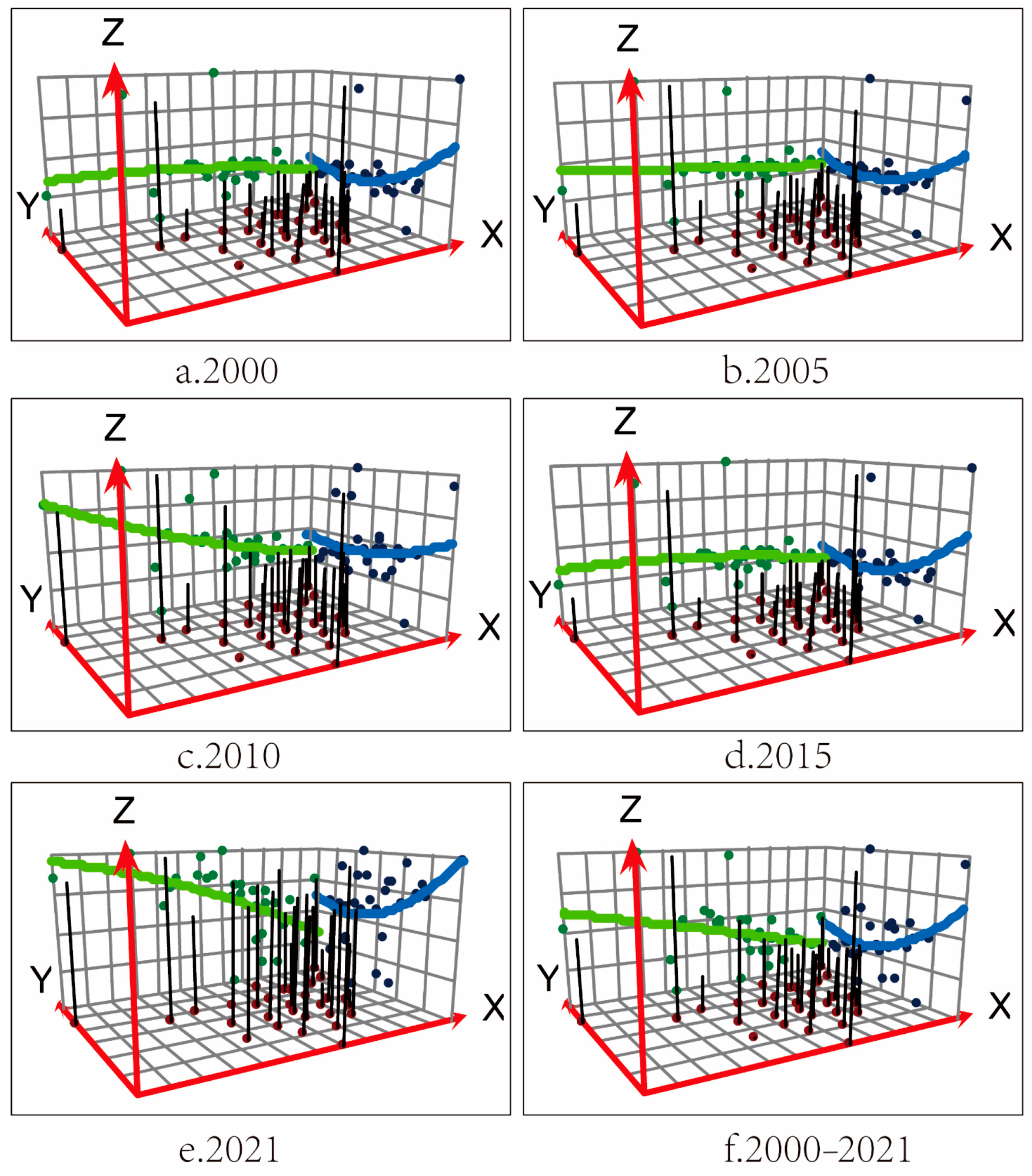
2.1.3. Trend Surface Analysis

The trend surface analysis method uses global polynomials to fit spatial sample point values with mathematical functions, transforming the two-dimensional spatial sample data into a three-dimensional visualized smooth curve that illustrates the spatial variation trends of geographical factors. This study applies trend surfaces to express the spatial differentiation trend of AEE in China. Here, Zi (xi, yi) represents the true observed value of the i-th geographical factor, and Ti (xi, yi) the fitted value from the trend surface, as given by the following formula [25]:

$$Z_i\left(x_i, y_i\right)=T_i\left(x_i, y_i\right)+{\epsilon }_i$$

(7)

In Equation (7), (x_i, y_i) represents the geographical coordinates, and i denotes the residual, which is the deviation between the observed value and the fitted value.

2.1.4. Dagum Gini Coefficient and Its Decomposition

This study employs the Dagum Gini coefficient and its decomposition to examine the relative disparities in AEE across China’s provinces. The Dagum Gini coefficient encompasses the overall Gini coefficient (G), the intra-regional Gini coefficient (Gjj) for region j, and the inter-regional Gini coefficient (Gjh) between regions j and h. The total contribution to disparities can be decomposed into three components using the sub-sample decomposition method: the intra-regional disparity contribution (Gw), the inter-regional disparity contribution (Gnb), and the contribution of hyper-variation density (Gt) [26], as expressed by:

$$G=G_w+G_{nb}+G_t$$

(8)

$$G={\displaystyle \frac{{\displaystyle \sum _{j=1}^k{\displaystyle \sum _{h=1}^k{\displaystyle \sum _{i=1}^{n_j}{\displaystyle \sum _{r=1}^{n_h}\left|Y_{ji}-Y_{hr}\right|}}}}}{2n^2\overline{Y}}}$$

(9)

$$G_{jj}={\displaystyle \frac{\frac{1}{2\overline{Y}}{\displaystyle \sum _{i=1}^{n_j}{\displaystyle \sum _{r=1}^{n_j}\left|Y_{ji}-Y_{jr}\right|}}}{{n_j}^2}}$$

(10)

$$G_{jh}={\displaystyle \frac{{\displaystyle \sum _{i=1}^{n_j}{\displaystyle \sum _{r=1}^{n_j}\left|Y_{ji}-Y_{hr}\right|}}}{n_j{n}_h(\overline{Y_j}+\overline{Y_h})}}$$

(11)

$$G_w={\displaystyle \sum _{j=1}^k{G}_{jj}{p}_j{s}_j}$$

(12)

$$G_{nb}={\displaystyle \sum _{j=2}^k{\displaystyle \sum _h^{j-1}{G}_{jh}(p_j{s}_h+p_h{s}_j)D_{jh}}}$$

(13)

$$G_t={\displaystyle \sum _{j=2}^k{\displaystyle \sum _{h=1}^{j-1}{G}_{jh}(p_j{s}_h+p_h{s}_j)(1-D_{jh})}}$$

(14)

$$p_j={\displaystyle \frac{n_j}{\overline{Y}}},s_j={\displaystyle \frac{n_j\overline{Y_j}}{nY}}, j=1,2,\dots \dots ,k$$

(15)

$$D_{jh}={\displaystyle \frac{d_{jh}-p_{jh}}{d_{jh}+p_{jh}}}$$

(16)

$$d_{jh}={\displaystyle {\int }_0^{\infty }d{F}_j(y){\displaystyle {\int }_0^y(y-x)d{F}_h}}(x)p_{jh}$$

(17)

$$\overline{Y_h}\ge \dots \ge \overline{Y_j}\ge \dots \ge \overline{Y_k}$$

(18)

In Equation (9), Y_ji represents the AEE of province i in region j; n is the number of provinces; k is the number of regions; d_jh measures the relative influence between regions j and h, and P_jh is the expected value for all cases where Y_ji − Y_hr < 0; F denotes the cumulative distribution function for each region. Equation (18) ranks the mean AEE of the regions.

2.1.5. Kernel Density Estimation Method

The kernel density estimation (KDE) method is a non-parametric test that does not assume any specific data distribution [27]. It derives a probability density function based on sample data and the kernel function K (x). Subsequently, the dynamic evolutionary trends of AEE are analyzed through the characteristics of the density curve, such as distribution shape, extensibility, and peaks. The probability density function is as follows:

$$f_n(x)={\displaystyle \frac{1}{nh}}{\displaystyle \sum _{i=1}^{n}K(\frac{p_i-x}{h})}$$

(19)

In Equation (18), x represents the sample mean, n denotes the number of observed sample values, h is the smoothing parameter (h > 0), where larger h values produce smoother data, and pi is a data point within the sample. The constraints for K (x) are as follows:

$$s.t.\left\{\begin{array}{l}\underset{x\to \infty }{\lim }K(x)•x=0\\ K(x)\ge 0,{\displaystyle {\int }_{-\infty }^{+\infty }K(x)dx=1}\\ \sup K(x)<+\infty ,{\displaystyle {\int }_{-\infty }^{+\infty }K(x)dx=1}\end{array}\right.$$

(20)

The Gaussian density function is used as the kernel function:

$$K(x)={\displaystyle \frac{1}{\sqrt{2\pi }}}\exp (-{\displaystyle \frac{x^2}{2}})$$

(21)

2.1.6. Geodetector

Geodetector is a statistical method used to detect spatial differentiation and its driving factors. It is a tool to figure out what drives differences in efficiency—like whether fertilizers or pesticide matters more. A challenge here is that we have to group data (like rainfall amounts) into categories, which might miss some details. Also, it assumes these patterns stay steady across space, which might not hold true when farming practices change fast. For Geo-detector models, following previous research, performing analyses at multiple spatial scales and carefully discretizing continuous data into meaningful categories (e.g., quantile-based classification or natural breaks) are recommended strategies to address spatial scale sensitivity and data classification biases [28]. Furthermore, statistical approaches such as permutation tests can reinforce the robustness and validity of Geo-detector findings by guarding against false-positive results due to random chance [29,30]. The underlying assumption is that if an independent variable significantly influences a dependent variable, then both should exhibit similar spatial distributions [31]. Typically, Geodetector discretizes ordinal, ratio, or interval variables (x_i, x_j) appropriately, and by calculating and comparing the q-values of individual factors as well as the q-value after their interaction, it determines whether an interaction exists between the two factors, along with the strength, direction, and whether the interaction is linear or nonlinear. This method is used to uncover the driving factors behind the spatial differentiation of the dependent variable. The q-value calculation formula is:

$$q=1-{\displaystyle \frac{{\displaystyle \sum _{k=1}^m{n}_k{{\sigma }_k}^2}}{n{\sigma }^2}}$$

(22)

In Equation (21), k represents the partition of the dependent variable Y (k = 1, 2, …, m), n denotes the sample size, 2 represents the total variance of Y, n_k is the sample size in partition k, and k² denotes the variance of Y in partition k. The criteria for determining the interaction term detection results are as follows:

$$q(x_i\cap x_j)<\mathit{Min}\left(q\right(,q\left(x_j\right)) \mathrm{Nonlinear} \mathrm{weakening}$$

$$\mathit{Min}\left(q\right(,q\left(x_j\right))<q(x_i\cap x_j)<\mathit{Max}\left(q\right(,q(x_j\left)\right) \mathrm{Single}-\mathrm{factor} \mathrm{nonlinear} \mathrm{weakening}$$

$$q(x_i\cap x_j)>\mathit{Max}\left(q\right(,q\left(x_j\right)) \mathrm{D}\mathrm{u}\mathrm{a}\mathrm{l}-\mathrm{f}\mathrm{a}\mathrm{c}\mathrm{t}\mathrm{o}\mathrm{r}\mathrm{e}\mathrm{n}\mathrm{h}\mathrm{a}\mathrm{n}\mathrm{c}\mathrm{e}\mathrm{m}\mathrm{e}\mathrm{n}\mathrm{t}$$

(23)

$$q(x_i\cap x_j)>\mathit{Max}\left(q\right(,q\left(x_j\right)) \mathrm{Independence}$$

$$q(x_i\cap x_j)=q\left(x_i\right)+q\left(x_j\right) \mathrm{Nonlinear} \mathrm{enhancement}$$

Nonlinear Weakening: when two factors combined yield less explanatory power than the sum of their individual effects, indicating interference that diminishes their joint impact. Single-Factor Nonlinear Weakening: when increasing a single factor results in a less-than-proportional gain in explanatory power, reflecting diminishing returns. Dual-factor enhancement: when two factors exhibit a simple additive or multiplicative effect when considered together. Independence: when two factors operate without interacting, so their combined effect equals the simple sum of their individual effects. Nonlinear enhancement: when two factors work together, their combined explanatory power exceeds the sum of their individual effects, indicating a strong synergistic effect.

2.1.7. Visual Representation of Models

To make the EBM and Geo-detector models easier to understand, we provide flowcharts illustrating their processes (Figure 1):

2.2. Indicator Selection and Data Sources

The essence of AEE is to achieve the maximum possible agricultural economic output and ecological protection with minimal agricultural resource inputs and environmental costs, reflecting the coordinated and mutually beneficial relationship between agricultural economy, resource utilization, and environmental protection. The selection of evaluation indicators for AEE in this study was based on the agricultural input-output indicator system proposed in the relevant literature [8,12]. Considering data availability and statistical consistency, land, labor, mechanical power, irrigation, fertilizers, and pesticides were selected as input indicators for regional agricultural factors, while total agricultural output value was used as the desired output indicator. For undesired output indicators, this study referred to the carbon emission model and estimation coefficients provided by Li Bo et al. [32]. Six categories of direct or indirect carbon emissions were considered, i.e., fertilizers, pesticides, agricultural films, diesel, electricity and water consumption for irrigation, and tillage-related losses. Based on the referenced study, the emission coefficients for the six major carbon sources were 0.8956 (kg/kg) for fertilizers, 4.9341 (kg/kg) for pesticides, 5.18 (kg/kg) for agricultural films, 0.5927 (kg/kg) for diesel, 20.476 (kg/hm²) for agricultural irrigation, and 312.6 (kg/km²) for agricultural tillage. The final AEE indicator system for China is presented in

Table 1. AEE measurement index system.

Indicator	Variables	Variables Description
Land input	Total crop sowing area (km2)	Reflects the actual cultivated area in agricultural production
Labor input	Agricultural labor force (per 10,000 people)	Converted based on the number of workers in the primary sector (gross agricultural output/gross rural agriculture, forestry, animal husbandry, and fishery output)
Machinery input	Total agricultural machinery power (per 10,000 kW)	Agricultural machinery is a representative tool of agricultural modernization
Water input for production factors	Effective irrigation area (per km2)	Agricultural water use is primarily for irrigation, which is used as a proxy
Fertilizer input	Amount of chemical fertilizers applied (10,000 tons, adjusted to pure content)	The inputs of fertilizers, pesticides, agricultural films, diesel, etc., are the main sources of pollution in agricultural production
Pesticide input	Pesticide usage (10,000 tons)
Agricultural film input	Agricultural film usage (10,000 tons)
Energy input	Amount of agricultural diesel used (10,000 tons)
Desirable output	Total agricultural output (in 100 million yuan)	Adjusted to constant 2000 prices using the CPI index to eliminate the impact of price changes
Undesirable output	Carbon emissions	Explained in the text

.

AEE is influenced by the interactions and feedback mechanisms among various factors involved in agricultural production and management. In this study, the driving factors are classified into agricultural production factors, socioeconomic factors, and natural environmental factors. Agricultural production factors include cropping intensity, cropping structure, agricultural mechanization intensity, and fertilizer usage per mu. Socioeconomic factors comprise urbanization rate, per capita disposable income of rural residents, the proportion of agricultural fiscal support, and average years of education. Natural environmental factors include disaster rate, average precipitation, and temperature. The complex interactions and interdependencies among these factors collectively determine the spatial and temporal differentiation of AEE [11,32,33,34]. A detailed explanation of the indicators is presented in

Table 2. Factors affecting AEE and classification.

Symbol	Meaning	Category	Category Description
URBAN	Urban population/total population at year-end	5	<10%; 10~30%; 30~50%; 50~70%; >70%
MCI	Average number of crop plantings per year on the same plot of land	5	<100%; 100~120%; 120~150%; 150~180%; >180%
PS	Area of food crop cultivation/area of non-food crop cultivation	8	Equal interval classification
pCDI	Per capita disposable income of rural residents	5	Natural breakpoint method
SOFSTA	Fiscal expenditure on agriculture, forestry, and water affairs/total sown area of crops	6	Natural breakpoint method
GDA	Disaster-affected agricultural area/total sown area of crops	5	Natural breakpoint method
MECH	Total agricultural machinery power/total sown area of crops	8	Equal interval classification
FUPA	Total fertilizer use/cultivated land area	3	<300; 300~500; >500
AYOS	(Number of primary school students × 6 + number of middle school students × 3 + number of high school students × 3 + 12 + number of students with higher education)/total population	5	<6; 6~7; 7~8; 8~9; >9
PRE	Average precipitation	6	Natural breakpoint method
TEM	Temperature	6	Natural breakpoint method

.

The study sample comprises 30 provinces in mainland China. Due to data availability constraints and the unique agricultural production conditions in Tibet, Hong Kong, Macau, and Taiwan, these regions were excluded from the empirical analysis. The study period spans from 2000 to 2021, covering the post-reform era. Data for the variables were sourced from the China Rural Statistical Yearbook, China Agricultural Statistical Data, Fifty Years of Agricultural Statistics of New China, provincial statistical yearbooks, 60-year statistical records, and the National Bureau of Statistics website (http://data.stats.gov.cn/easyquery.htm?cn=E0103 (accessed on 5 May 2023)). Missing data were supplemented using interpolation methods, yielding a 21-year panel dataset.

3. Measurement and Spatial Distribution Dynamics of AEE in China

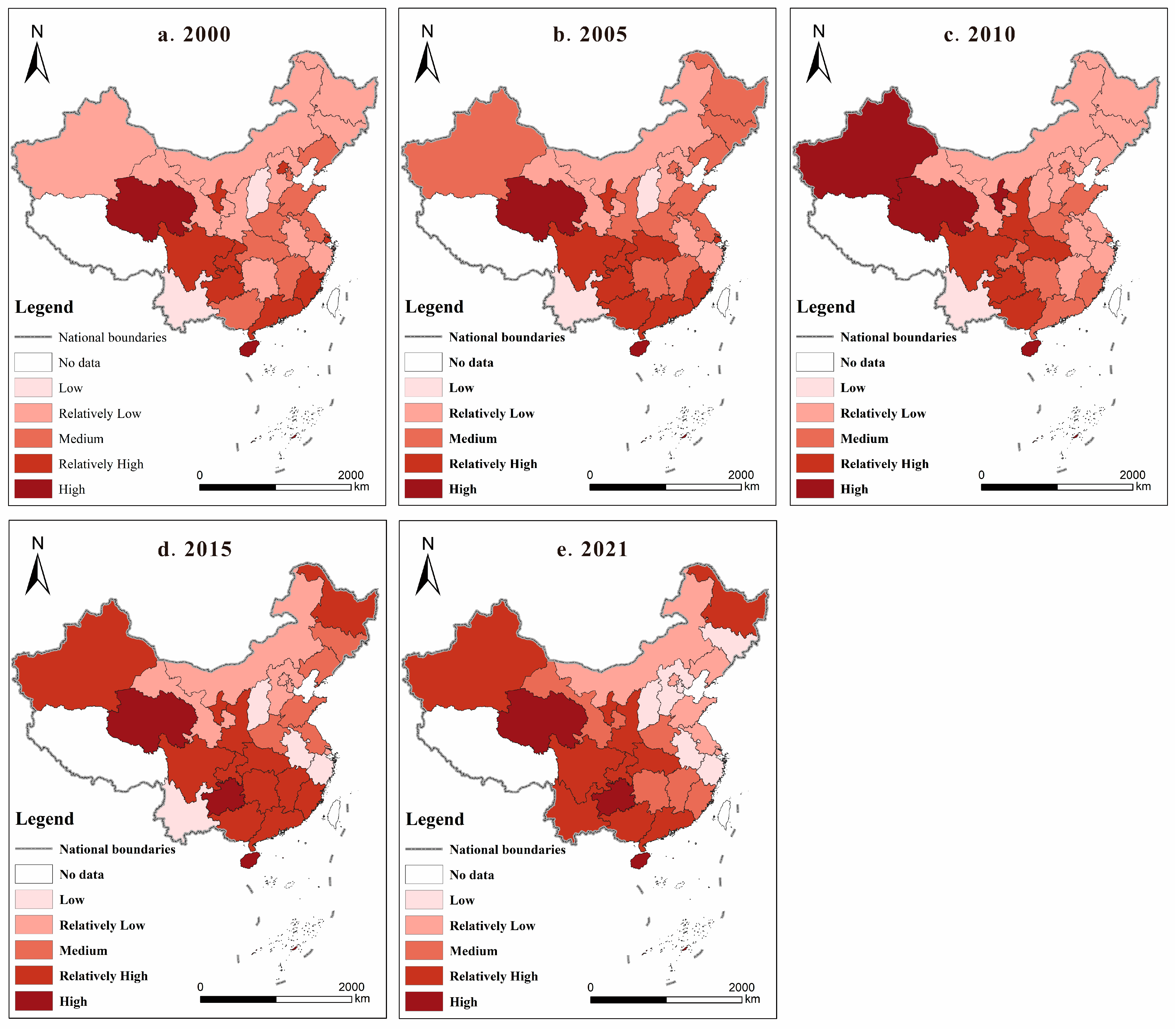
3.1. Measurement and Evaluation of AEE in China

From 2000 to 2021, China’s AEE exhibited a steady upward trend (Figure 2a), increasing from 0.504 in 2000 to 1.038 in 2021, with an average annual growth rate of 4.82%. As shown by the regional evolution process (Figure 2b), AEE in the western region was significantly higher than that in the central and eastern regions, with the eastern region slightly surpassing the central region. This pattern reveals a path-dependent characteristic of AEE’s spatiotemporal evolution, with the hierarchical structure remaining stable across regions. In terms of the disparity evolution process, the growth rate of AEE in the western region markedly outpaced that of the eastern and central regions, resulting in a widening gap over time. This reflects the problem of slow improvement in AEE in the eastern and central regions, particularly in the central region, which appears to be stuck in an “AEE improvement trap”.

Table 3. AEE of 30 provincial-level administrative units in China.

Tier	Zone	Province (Autonomous Region, Municipality)	Mean	Ranking
First Tier	Western	Qinghai	1.1940	1
	Eastern	Hainan	1.1575	2
Second Tier	Western	Ningxia	0.8778	3
	Western	Guizhou	0.8615	4
	Western	Xinjiang	0.8492	5
	Western	Sichuan	0.8438	6
	Western	Guangxi	0.8238	7
	Central	Hubei	0.8173	8
	Western	Chongqing	0.8139	9
	Eastern	Guangdong	0.8129	10
	Western	Shaanxi	0.8044	11
	Eastern	Fujian	0.7900	12
	Eastern	Heilongjiang	0.7776	13
	Central	Jiangxi	0.7397	14
	Central	Hunan	0.7326	15
	Central	Henan	0.7110	16
	Eastern	Shanghai	0.7082	17
Third Tier	Eastern	Beijing	0.6933	18
	Eastern	Jiangsu	0.6856	19
	Eastern	Shandong	0.6845	20
	Eastern	Liaoning	0.6753	21
	Western	Gansu	0.6375	22
	Western	Inner Mongolia	0.6363	23
	Eastern	Jilin	0.6278	24
	Eastern	Hebei	0.6259	25
	Eastern	Tianjin	0.6255	26
	Eastern	Zhejiang	0.5600	27
	Central	Anhui	0.5405	28
	Central	Shanxi	0.4846	29
	Western	Yunnan	0.4809	30

Note: In the “Region” column, 1 represents the Eastern region, 2 represents the Central region, and 3 represents the Western region.

presents the ranking of average AEE in China’s provinces from 2000 to 2021. The data indicate a generally stable pattern over this period. Qinghai and Hainan emerged as the top-tier regions, with mean efficiency values of 1.1940 and 1.1575, respectively. As regions with distinctive geographic features, Qinghai and Hainan have leveraged their resource advantages, adopting divergent approaches that yielded comparable outcomes in AEE. Qinghai’s plateau climate and relatively pristine environment contributed to maintaining ecological balance in agricultural production. In contrast, Hainan capitalized on its warm and humid climate to develop diversified crop-planting models and eco-friendly agricultural practices, positioning itself as a high-efficiency region. The second tier includes Ningxia, Guizhou, Xinjiang, Sichuan, Guangxi, Hubei, Chongqing, Guangdong, Shaanxi, Fujian, Heilongjiang, Hunan, Henan, and Shanghai, with mean efficiency values ranging between 1 and 0.7. The remaining provinces constitute the third tier, where average efficiency values were below 0.7. Shanxi and Yunnan ranked at the bottom, with mean values below 0.5. The persistently low AEE in Shanxi and Yunnan is primarily attributed to their relatively lagging economic development, single-dimensional agricultural industry structures, and low ecological benefits. Additionally, unfavorable resource endowments and land use patterns further constrained efficiency. For instance, soil desertification and water erosion issues in Shanxi hindered agricultural development, while Yunnan’s mountainous and plateau terrain lacked the basic conditions for agricultural expansion.

Based on spatial-temporal evolution maps (Figure 3) and three-dimensional trend charts (Figure 4) generated using ArcGIS, it can be observed that China’s AEE significantly improved between 2000 and 2021. The national average AEE reached 1.0384 in 2021, an increase of 106.04% compared to 2000. The overall spatial distribution exhibited a weakening pattern from west to east and from south to north. Trend analysis revealed a “same level—higher in the west and lower in the east” pattern along the east–west axis and a “U-shaped—smooth—U-shaped” transformation along the north–south axis in 2000, 2005, 2015, and 2021. This evolutionary process indicated that AEE was higher in the western and southern regions than in the eastern and northern regions. Additionally, growth in AEE in Northeast China was notably slow, underscoring the widening spatial disparities between west and east, as well as south and north. From the perspectives of natural characteristics and industrial structure, the persistent spatial differences can be attributed to the resource advantages in western and southern regions, exemplified by Qinghai, Guizhou, Guangdong, and Guangxi. These regions are rich in ecological resources, including water, land, and biodiversity, which facilitate diversified agricultural structures and cropping systems (e.g., crop farming, animal husbandry, and agroforestry systems), thereby enhancing overall resource efficiency. In contrast, eastern and northern regions are dominated by secondary and tertiary industries, such as manufacturing and services in the east and traditional crop farming in the northeast, resulting in lower AEE.

The spatial evolution process (Figure 2b) shows that AEE in western China is significantly higher than that in central and eastern regions, with eastern regions slightly outperforming central ones. This pattern suggests a path-dependent characteristic, as the relative strengths among these regions have remained spatially stable. From the perspective of gap evolution, the growth rate of AEE in the western region has been markedly higher than in the eastern and central regions, leading to a widening gap over time. This trend highlights the slow improvement of AEE in the eastern and central regions, particularly in the central region, which appears to have fallen into an “AEE improvement trap”.

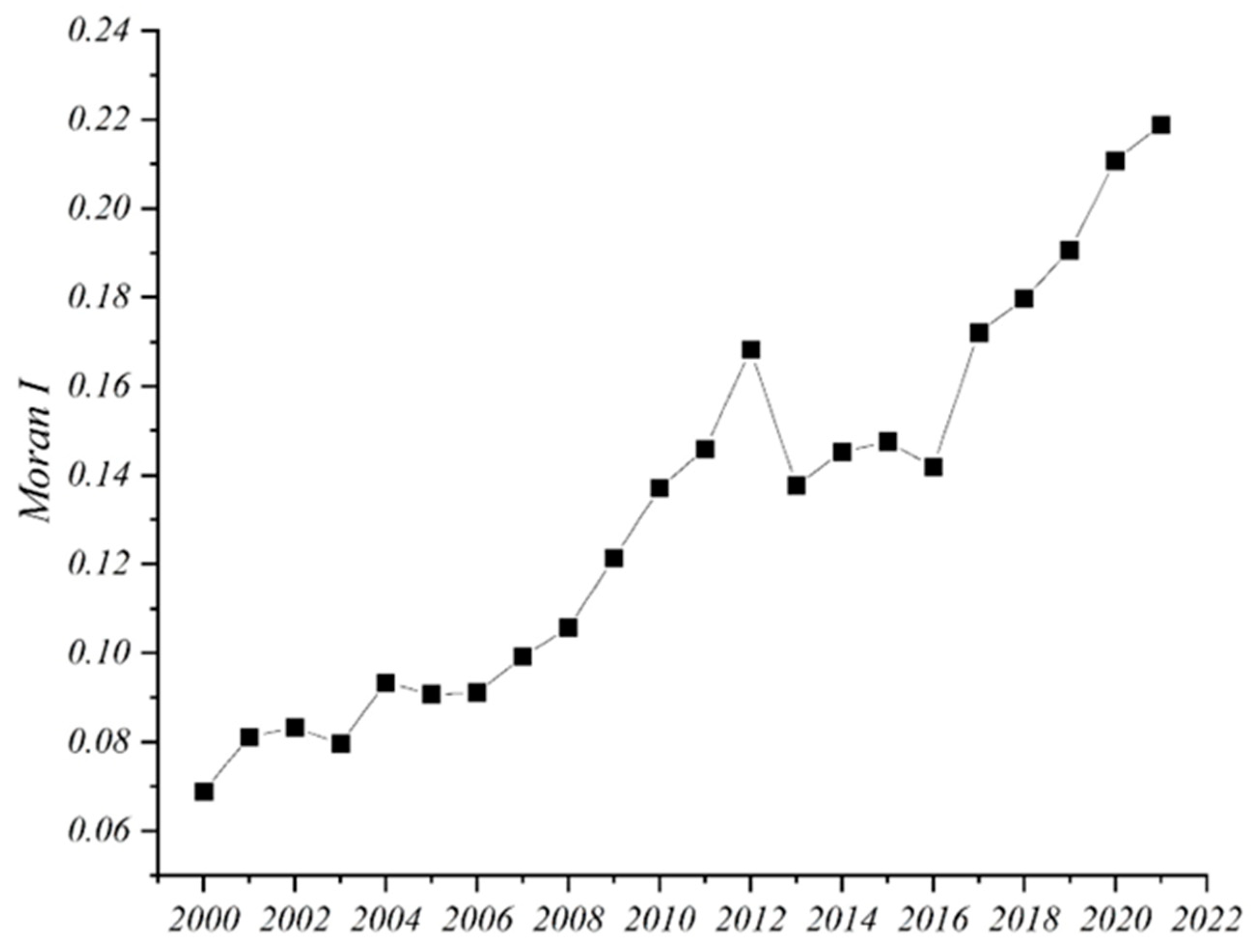
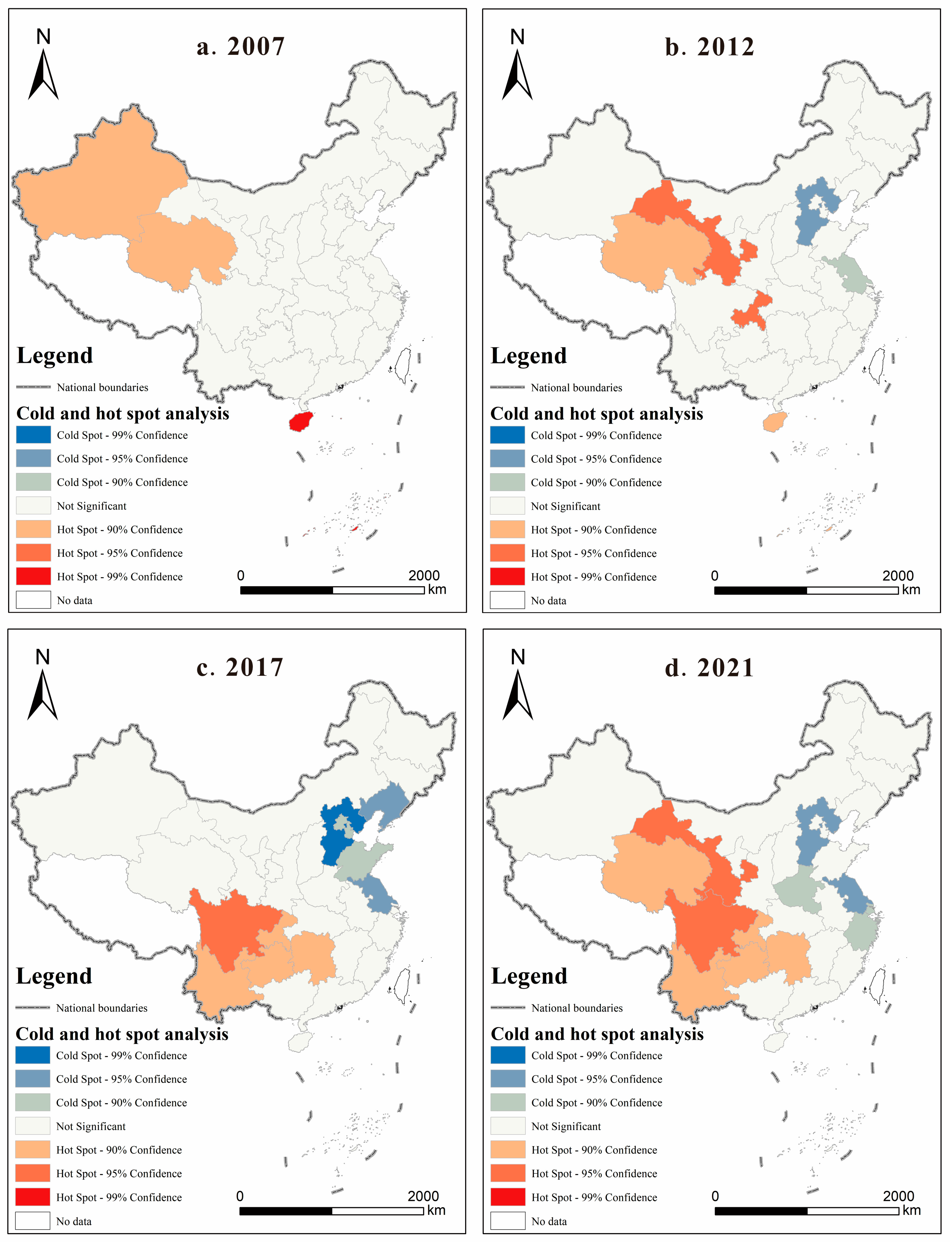
3.2. Spatial Correlation Analysis

To investigate the spatial correlation characteristics of China’s AEE, spatial autocorrelation analysis for the period 2000 to 2021 was conducted using ArcGIS 10.7.

Table 4. Spatial correlation of AEE in China.

Year	Moran I	Z	P
2000	0.0689	1.2951	0.1953
2001	0.0812	1.449	0.1473
2002	0.0832	1.4768	0.1397
2003	0.0796	1.4304	0.1526
2004	0.0934	1.6102	0.1074
2005	0.0907	1.571	0.1162
2006	0.0911	1.5723	0.1159
2007	0.0992	1.6741	0.0941
2008	0.1057	1.7543	0.0794
2009	0.1213	1.9528	0.0508
2010	0.1371	2.1336	0.0329
2011	0.1459	2.2368	0.0253
2012	0.1682	2.5140	0.0119
2013	0.1377	2.1316	0.0330
2014	0.1452	2.2285	0.0259
2015	0.1476	2.2604	0.0238
2016	0.1419	2.1856	0.0288
2017	0.1721	2.5693	0.0102
2018	0.1797	2.6741	0.0075
2019	0.1906	2.8213	0.0048
2020	0.2108	3.0950	0.0020
2021	0.2188	3.2155	0.0013

shows that Moran’s I indices remained positive and exhibited increasing fluctuations during this period. However, it was only after 2007 that AEE in China displayed significant spatial autocorrelation, indicating that in earlier years, AEE levels across regions were relatively independent without clear clustering or dispersion patterns. After 2007, spatial autocorrelation increased significantly, suggesting that AEE levels across regions became more similar, showing a certain degree of spatial correlation (Figure 5). As institutional barriers were gradually resolved, activities with positive spatial externalities, such as the spillover of agricultural cultivation technologies, contributed to an increasingly strengthened spatial association of AEE. This enhanced spatial correlation has helped regions move away from isolated development models and facilitated the coordinated allocation of agricultural resources across neighboring regions, promoting high-efficiency agricultural ecosystems.

Given that China’s AEE exhibited significant spatial clustering only from 2007 onward, this study selects the years 2007, 2012, 2017, and 2021 for hotspot and coldspot analysis (Figure 6). The findings indicate that in 2007, hotspot regions were primarily located in Xinjiang, Qinghai, and Hainan (Figure 6a). By 2012, AEE further strengthened while maintaining its overall spatial pattern, with Qinghai and Hainan remaining as hotspots and Jiangsu and Hebei emerging as new coldspot regions (Figure 6b). In 2017, high-clustered regions gradually shifted toward central areas, and high-efficiency regions such as Qinghai and Hainan disappeared, replaced by Sichuan, Yunnan, Chongqing, Guizhou, and Hunan. Low-clustered regions expanded to include Jiangsu, Shandong, Hebei, Tianjin, Beijing, and Liaoning (Figure 6c). By 2021, low-clustered regions had shifted toward central China, encompassing Zhejiang, Jiangsu, Shanghai, Henan, and Hebei (Figure 6d). Overall, high-clustered regions of AEE were primarily located in the western and central areas, particularly Hunan, while low-clustered regions were concentrated in the eastern and central areas, such as Henan. This pattern aligns with the spatial gradient decline of AEE from west to east.

4. Spatial Disparities and Their Origins in AEE in China

4.1. The Overall and Regional Differences in China’s AEE

Table 5. Overall and regional Gini coefficients of AEE in China.

Year	Overall	Eastern	Central	Western
2000	0.1343	0.1230	0.0798	0.1602
2001	0.1326	0.1044	0.0928	0.1706
2002	0.1298	0.1040	0.0808	0.1695
2003	0.1329	0.1049	0.0786	0.1719
2004	0.1201	0.0984	0.0691	0.1586
2005	0.1173	0.0954	0.0739	0.1501
2006	0.1150	0.0968	0.0722	0.1445
2007	0.1135	0.0935	0.0677	0.1452
2008	0.1161	0.0943	0.0671	0.1481
2009	0.1154	0.0960	0.0525	0.1491
2010	0.1333	0.0906	0.0773	0.1690
2011	0.1379	0.0906	0.1146	0.1572
2012	0.1386	0.1010	0.1153	0.1287
2013	0.1310	0.1050	0.1126	0.1195
2014	0.1277	0.1038	0.1208	0.1159
2015	0.1250	0.1023	0.1204	0.1160
2016	0.1276	0.1043	0.1225	0.1143
2017	0.1289	0.1261	0.1236	0.0779
2018	0.1204	0.1133	0.1224	0.0713
2019	0.1124	0.1106	0.1129	0.0622
2020	0.0998	0.1006	0.1064	0.0371
2021	0.0861	0.0858	0.0997	0.0335

illustrates the evolution of overall and intra- and inter-regional differences in AEE from 2000 to 2021. (1) Overall level: Over the 22-year period, the Gini coefficient of China’s AEE fluctuated irregularly between 0.0861 and 0.1386, decreasing by 35.91% by the end of the study period compared to the initial period, with an average value of 0.1225. This indicates a significant improvement in the equality of AEE. The Chinese government has implemented a series of robust policies and reforms to promote green agricultural development, including rural land system reforms, support for agricultural technological innovation, and ecological subsidies. These initiatives have not only enhanced the production capacity and competitiveness of agricultural producers but also promoted the equitable allocation of resources and improved the ecological environment. (2) Regional results: During the study period, the average Gini coefficients for the eastern, central, and western regions were 0.102, 0.0947, and 0.1259, respectively, with reductions of 30.23%, 24.94%, and 79.1% by the end of the study compared to the initial period. This suggests that the central region exhibited the highest level of equality in AEE, followed by the eastern region, with the western region lagging behind. The evolution trends of Gini coefficients in the eastern and central regions followed a “decline-rise-decline” pattern, while the western region displayed a steeper declining trend. These findings highlight the Chinese government’s emphasis on integrating sustainable development concepts that align with natural preservation and green agricultural development. Effective technological transfer and diffusion have gradually enabled the western region to catch up in agricultural technology, fostering resource-saving and nature-conserving production methods that enhance AEE.

4.2. Regional Differences in AEE in China

Table 6. Interval Gini coefficients and contribution of differences in AEE in China.

Year	East–Central	East–West	Central–West	Gw	Gnb	Gt
2000	0.1179	0.1449	0.1340	0.0488	0.0336	0.9176
2001	0.1140	0.1423	0.1447	0.0470	0.0308	0.9222
2002	0.1078	0.1412	0.1391	0.0463	0.0299	0.9237
2003	0.1141	0.1428	0.1468	0.0469	0.0326	0.9204
2004	0.0954	0.1327	0.1258	0.0432	0.0238	0.9330
2005	0.0992	0.1266	0.1267	0.0417	0.0267	0.9316
2006	0.1007	0.1233	0.1208	0.0411	0.0299	0.9290
2007	0.0951	0.1225	0.1232	0.0405	0.0254	0.9341
2008	0.0937	0.1262	0.1296	0.0411	0.0232	0.9357
2009	0.0852	0.1304	0.1257	0.0409	0.0227	0.9363
2010	0.0902	0.1576	0.1577	0.0440	0.0378	0.9182
2011	0.1088	0.1592	0.1667	0.0436	0.0366	0.9198
2012	0.1140	0.1624	0.1735	0.0414	0.0477	0.9108
2013	0.1169	0.1434	0.1669	0.0408	0.0448	0.9145
2014	0.1185	0.1398	0.1539	0.0402	0.0394	0.9204
2015	0.1204	0.1357	0.1441	0.0398	0.0333	0.9269
2016	0.1243	0.1409	0.1446	0.0400	0.0348	0.9252
2017	0.1296	0.1458	0.1482	0.0383	0.0563	0.9054
2018	0.1240	0.1344	0.1441	0.0351	0.0548	0.9101
2019	0.1257	0.1260	0.1214	0.0328	0.0471	0.9201
2020	0.1162	0.1152	0.1098	0.0270	0.0489	0.9241
2021	0.1003	0.0938	0.1035	0.0239	0.0440	0.9321

illustrates the evolution of regional disparities in China’s AEE from 2000 to 2021. Based on the average inter-regional Gini coefficients, the order was central-western (0.1387) > eastern-western (0.1358) > eastern-central (0.1096). In terms of variation rates, the decreases were eastern-western (−35.22%), central-western (−22.77%), and eastern-central (−14.93%). The ranking of average Gini coefficients indicates that AEE disparities were largest between the central and western regions, while the gap between the eastern and central regions was the smallest. From the perspective of variation rates, the eastern-western Gini coefficient experienced the largest decline at 35.22%, followed by a 22.77% decrease in the central-western gap. These findings suggest a dynamic convergence trend in China’s AEE over time, indicating that not only are intra-regional efforts contributing to the greening of agricultural development, but inter-regional linkages are also fostering a more balanced evolution of AEE.

Furthermore, Table 6 also illustrates the evolution of the sources of spatial differences in China’s AEE from 2000 to 2021. In terms of contributions, the super-variation density contribution rate was greater than the intra-regional difference contribution rate, which, in turn, exceeded the inter-regional difference contribution rate. Over the 22-year period, the average contribution rate of inter-regional differences was 3.67%, the average contribution rate of intra-regional differences was 4.02%, and the average super-variation density contribution rate was 92.32%. This indicates that extreme values of AEE are the primary source of the pronounced spatial differentiation in AEE in China. Specifically, during the 22 years, the contribution rate of intra-regional differences showed a fluctuating decline, with a reduction of 51.05% by the end of the study period compared to the beginning. Meanwhile, the contributions from inter-regional differences and super-variation density both showed an increasing trend, highlighting that the spatial disparities in AEE in China are not only dominated by extreme values, but also reflect a significant increase in the share of super-variation density contributions. Through the Dagum Gini coefficient decomposition, our analysis revealed that the regional disparities in AEE are predominantly driven by extreme values. This indicates that a significant gap exists between regions with high efficiency and those with low efficiency. For areas exhibiting strong polarization, we recommend that government interventions focus on providing enhanced technical and financial support to low-efficiency regions.

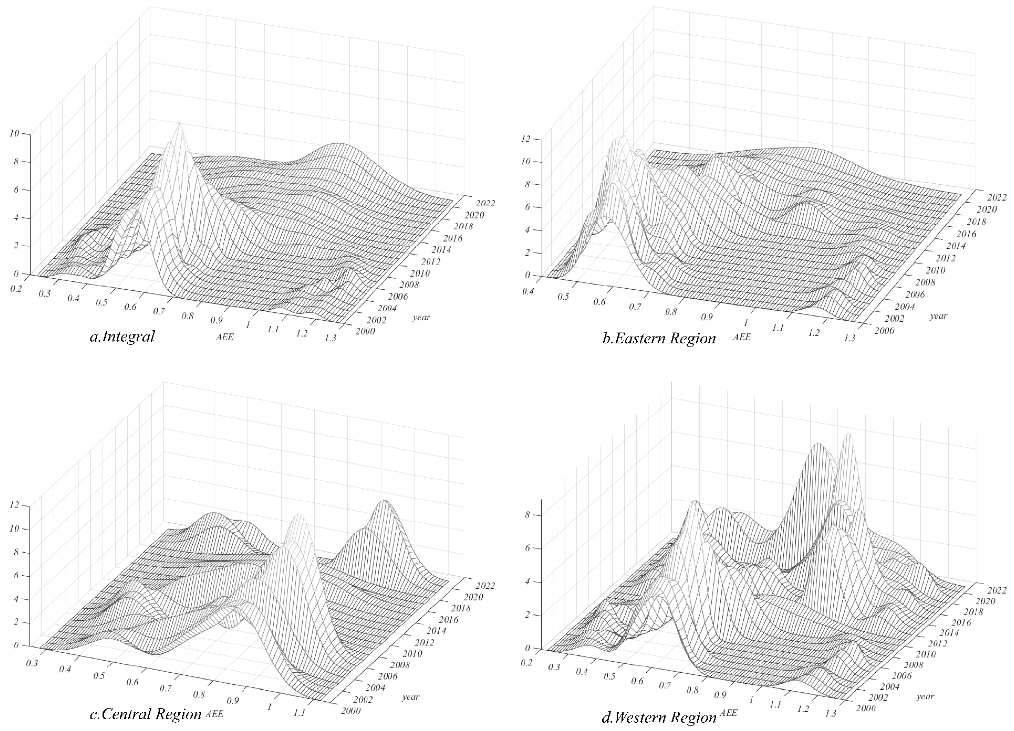
4.3. Absolute Differences in AEE in China

The use of kernel density estimation to characterize the evolution of absolute differences in China’s AEE can help mitigate the impact of unknown parameters on the estimation results [33,34,35]. (1) Overall level: Figure 7a illustrates the dynamic evolution of the AEE distribution across 30 regions in China during the study period. It is evident that, over the study period, the distribution center of China’s overall AEE curve has shifted to the right, the curve’s width has increased, and the peak height has notably decreased. This suggests an improvement in China’s overall AEE, accompanied by a significant reduction in absolute differences. The decline in peak height may indicate that more regions or farmers have relatively low AEE. The overall distribution shows a distinct rightward skew, and the distribution’s extent has broadened to some degree, indicating that the gap between provinces with high AEE and the average level continues to widen. Specifically, in terms of the evolutionary process, the peak height underwent an “increase-decrease” cycle. Before 2008, there was polarization in China’s AEE, which weakened after that period. (2) Eastern region (Figure 7b): The kernel density curve evolution in the eastern region from 2000 to 2021 mirrors the overall trend, with the curve’s distribution center shifting to the right, the peak height decreasing, and a rightward skew emerging. The double-peak feature was evident before 2018, indicating an overall improvement in AEE in the eastern region. The rightward skew implies the expansion of high-efficiency agricultural areas, with clear polarization in earlier years, though this characteristic weakened over time. (3) Central region (Figure 7c): From 2000 to 2021, the kernel density curve in the central region shifted its distribution center from left to right, with the curve’s width undergoing an “expansion-contraction” change. The double-peak (indicating the presence of two dominant efficiency clusters within a region) feature was prominent, with a decrease in peak height, indicating that AEE in the central region evolved from “decline to improvement.” However, the rate of improvement in the central region was slow. (4) Western region (Figure 7d): From 2000 to 2021, the kernel density curve in the western region showed an increase in peak height, with multiple peaks, and a rightward skew exhibiting a converging trend. This indicates significant internal absolute differences in AEE in the western region, with some low-efficiency agricultural areas still present, and a multi-polarization feature. In summary, although overall AEE in China has significantly improved with the deepening of the agricultural green development concept, there remains a slight trend toward unbalanced changes in the later stages. In terms of regional differences, the absolute disparity within the eastern region is widening, while the central and western regions exhibit characteristics of bi-polarization and multi-polarization, respectively. This could be due to the challenges faced by certain regions or farmers in terms of technology, resources, and environmental protection, leading to slow improvements in AEE. Overall, regions characterized by multipolarization require the formulation of differentiated policies that address the unique conditions of each sub-region. Significant differences in policy execution are evident among the eastern, central, and western regions. For western areas, we recommend further intensifying infrastructure development and technical support, whereas in central and eastern regions, the focus should be on optimizing agricultural structures and enhancing resource-use efficiency. For example, while the “Western Development Strategy” has, to some extent, promoted infrastructure construction in the west, it may also lead to imbalances in resource allocation. Consequently, future policies should emphasize interregional coordination, optimize resource distribution, and foster balanced development across regions.

5. Drivers of Spatiotemporal Differentiation in AEE in China

The Geodetector model was used to analyze the linear driving effects of various factors on the spatiotemporal differentiation of China’s AEE (

Table 7. Determinants of the spatiotemporal evolution of AEE in China.

	2000		2005		2010		2015		2021
	q	p	q	p	q	p	q	p	q	p
URBAN	0.057	0.000	0.144	0.000	0.340	0.000	0.316	0.000	0.209	0.000
MCI	0.196	0.000	0.058	0.000	0.601	0.000	0.307	0.000	0.191	0.000
PS	0.526	0.000	0.588	0.000	0.108	0.000	0.029	0.000	0.201	0.000
pCDI	0.043	0.000	0.029	0.000	0.113	0.000	0.133	0.000	0.295	0.000
SOFSTA	0.154	0.000	0.711	0.000	0.500	0.000	0.520	0.000	0.225	0.000
GDA	0.262	0.000	0.317	0.000	0.379	0.000	0.130	0.000	0.099	0.000
MECH	0.324	0.000	0.344	0.000	0.225	0.000	0.105	0.000	0.081	0.000
FUPA	0.167	0.000	0.190	0.000	0.231	0.000	0.180	0.000	0.286	0.000
AYOS	0.027	0.000	0.171	0.000	0.499	0.000	0.192	0.000	0.172	0.000
PRE	0.110	0.000	0.170	0.000	0.093	0.000	0.217	0.000	0.431	0.000
TEM	0.207	0.000	0.207	0.000	0.237	0.000	0.291	0.000	0.114	0.000

). Table 7 presents the driving forces of various factors in 2000, 2005, 2010, 2015, and 2021, with results passing the 1% significance level test, indicating that these factors have a significant determinative effect on the spatiotemporal differentiation of China’s AEE. Over time, the driving effects of the crop rotation index, planting structure, disaster rate, agricultural machinery intensity, and temperature showed an “increase-then-decrease” evolutionary trend. The degree of influence decreased by 2.55%, 61.79%, 62.21%, 75%, and 44.93%, respectively, compared to the early years, indicating that the explanatory power of planting structure, disaster rate, agricultural machinery intensity, and temperature decreased most significantly in relation to the spatiotemporal differentiation of China’s AEE. In contrast, the explanatory power of urbanization rate, rural per capita disposable income, proportion of fiscal expenditure on agriculture, fertilizer use, average years of education, and precipitation on the spatiotemporal differentiation of China’s AEE showed varying degrees of enhancement. Notably, urbanization rate, rural per capita disposable income, average years of education, and precipitation showed the most significant increases, growing by 266.67%, 586.05%, 537.04%, and 291.82%, respectively, in 2021 compared to 2000. These results indicate that, with the development of agriculture in China, exogenous differences are gradually being leveled out, and AEE is increasingly determined by regional endowments and natural climatic factors, such as urbanization rate and precipitation. Specifically, with the improvement of agricultural varieties, the upgrading of disaster prevention and control, and the widespread use of agricultural machinery, differences among regions in these factors are narrowing, weakening their determinative power on spatiotemporal differentiation. Instead, local fiscal levels, farmers’ individual endowments, and climatic factors are playing a greater role in driving the spatiotemporal differentiation of AEE in China.

To further investigate the explanatory power of factor interactions on AEE and identify the types of interactions, an interaction term detector was used to analyze the interactions between factors in 2000, 2005, 2010, 2015, and 2021. The results of the detection are shown in Figure 8. From the perspective of the evolution of interaction types, between 2000 and 2021, the interaction between any two factors enhanced the explanatory power of either factor on the spatial differentiation of the digital economy. The interactions primarily manifested as two types: factor enhancement and nonlinear enhancement. The evolution of interaction types was dominated by a pattern of “nonlinear enhancement–two-factor enhancement–nonlinear enhancement”, with spatial differentiation in each period being primarily driven by different two-factor interactions. From the perspective of the evolution of explanatory power of interactions: in 2000, the interaction between per capita rural disposable income and fertilizer usage was the primary driving force behind spatiotemporal differentiation, with an explanatory power of 0.944 (Figure 8a). In 2005, the interactions between planting structure and urbanization rate, planting structure and fiscal agricultural support, disaster rate and urbanization rate, agricultural machinery intensity and disaster rate, average years of education and disaster rate, and average years of education and fiscal agricultural support all exceeded 0.9, making them the primary driving factors behind spatial differentiation that year (Figure 8b). In 2010, the interaction between the cropping index and planting structure and the interaction between the cropping index and average years of education were the primary determinants of spatial differentiation (Figure 8c). In 2015 and 2021, the spatiotemporal differentiation of China’s AEE was primarily driven by the interactions between precipitation and urbanization rate and between disaster rate and urbanization rate, with explanatory powers of 0.944 and 0.818, respectively (Figure 8d,e). In summary, the spatiotemporal differentiation of China’s AEE was initially driven by the interaction between rural disposable income and fertilizer usage, then by the interactions among cropping index, planting structure, urbanization rate, fiscal agricultural support, and average years of education in the middle period, and later evolved to be predominantly driven by the interactions between precipitation, urbanization rate, and disaster rate. When two factors exhibit complementary and multiplicative effects, they mutually complement and reinforce each other, jointly promoting AEE and enhancing the explanatory power of spatial differentiation. For example, the combined effect of fiscal agricultural support and average years of education can accelerate the improvement of AEE. High levels of human capital enable farmers to absorb agricultural technological knowledge, and government fiscal spending on agricultural technical training complements farmers’ human capital, creating a positive feedback loop for the improvement of AEE, thereby enhancing the spatial differentiation of the digital economy.

6. Discussion

This study, based on the foundational indicator data from 30 provinces (municipalities and autonomous regions) in China from 2000 to 2021, used the undesirable output super-efficiency EBM theoretical model to measure the AEE of each province. Through trend surface analysis, spatial correlation analysis, Dagum Gini coefficient and its decomposition, and kernel density analysis, this study systematically reveals the spatial characteristics and intra- and inter-regional differences of AEE in China and further analyzes the driving factors and their interaction effects on the spatiotemporal differentiation of AEE using the geographical detector.

In terms of spatial patterns, spatial differences, and spatial agglomeration, there is both consistency and divergence between the findings of this study and existing research. First, in terms of spatial patterns, despite differences in efficiency measurement theories and methods in the academic community, this study concludes that the overall AEE in China has significantly improved, albeit with regional differences, a conclusion that is in line with several studies [34,36,37]. This suggests that under China’s rapid economic development and policy support, AEE has gradually increased. Specifically, the AEE performance of each province during the study period shows that provinces such as Qinghai and Hainan consistently lead in AEE, a result that is consistent with the research of Wang Yaqin and colleagues [12]. This indicates that these regions demonstrate significant advantages in improving AEE, possibly due to their unique natural resources and policy support. Additionally, the study found that AEE in China exhibits a clear gradient feature, with a spatial pattern of decreasing AEE from west to east and from south to north, which is consistent with the findings of Chen and Liao [9,38]. Second, in terms of spatial differences, this study concludes that the internal differences in the western and eastern regions have decreased, while internal differences in the central region have increased. The difference between the western region and the other two regions showed a divergent trend, and the polarization between the eastern and central regions weakened. The western region exhibited significant absolute differences and an enhanced multipolar differentiation feature. These results enrich the existing literature on the spatial differences in China’s AEE from the perspective of difference decomposition, but show some divergence from previous studies [34,38]. This divergence may be due to differences in the methods, data span, and regional division used by different authors. Finally, in terms of spatial agglomeration, this study found that after 2007, there was a significant positive spatial correlation in AEE in China, with both coldspots and hotspots increasing. This result is consistent with the findings of Wang et al. [39] but diverges from the conclusions of Zeng et al. [40], likely due to differences in the methods and scope of spatial disparity studies. This study used geographic detector to further reveal the interactions between various driving factors, a method that departs from traditional univariate studies and focuses on isolating key factors and their interactive effects on the spatiotemporal differentiation of AEE in China. The study shows that socio-economic factors such as urbanization rate, per capita disposable income of rural residents, and the proportion of fiscal subsidies for agriculture play a significant role in improving AEE, while the explanatory power of technical factors, such as agricultural machinery intensity and cropping structure, has diminished. This finding enriches and deepens existing research on the spatiotemporal differentiation of AEE in China. Our findings offer actionable insights for policy. The west-to-east AEE decline suggests prioritizing resource allocation to eastern and central regions, where growth is slow, through investments in precision agriculture to boost efficiency without environmental costs. The strong influence of urbanization and education highlights the need for integrated rural training programs, such as subsidies for farmers attending ecological farming workshops in nearby cities. The dominance of super-variation density in spatial disparities calls for targeted interventions in low-efficiency provinces like Shanxi and Yunnan—e.g., pilot projects for organic farming or agroforestry—to reduce polarization. In high-AEE regions like Qinghai, scaling up plateau-adapted crop rotation practices to other western provinces, supported by the 14th Five-Year Plan, could amplify gains. To assess the robustness of our findings over an extended period, we consolidated previous research on China’s AEE. Liu et al. (2020) performed a subperiod analysis of agricultural eco-efficiency in China and found that, even under significant external disturbances, the efficiency trends maintained their overall pattern [11]. Likewise, Wang et al. (2021) observed that major policy interventions did not significantly alter the long-term evolution of AEE [12]. These findings support the robustness of our results and suggest that our conclusions are not driven solely by transient external shocks or specific policy changes.

Despite the progress made in measuring AEE and analyzing its spatiotemporal differentiation, there are still certain limitations in this study. First, at the theoretical and data levels, this study defined agricultural carbon emissions as undesirable outputs. However, in reality, pesticide residues, soil and water pollution, and other factors are also undesirable outputs of agricultural production. Due to limitations in data availability (with the study period spanning from 2000 to 2021), the latest trends in AEE could not be captured. Second, although this study provided an in-depth analysis of the development status of AEE in China, it lacked detailed case studies of specific provinces or regions. Finally, although this study revealed the interaction of multiple driving factors, the explanation of their mechanisms remains preliminary, especially the lack of a detailed analysis of the micro-mechanisms underlying regional differentiation. This result may lead to policies for improving regional AEE that are insufficiently specific. In summary, despite these shortcomings, this study, through systematic spatiotemporal analysis and exploration of driving factors, provides new perspectives on understanding the evolution of AEE in China and offers valuable insights for the formulation of policies to enhance AEE. Future research should further deepen the connotation and extension of undesirable agricultural outputs, improve data, conduct differentiated analysis of regional AEE, and implement targeted policies to promote the high-quality sustainable development of Chinese agriculture.

7. Conclusions and Policy Recommendations

7.1. Conclusions

This study assessed China’s AEE from 2000 to 2021 across 30 provinces using the super-efficiency EBM and Geo-detector models. Key findings include: (1) AEE improved significantly, with a west-to-east and south-to-north decline, showing path dependence and widening regional gaps, notably with high-efficiency clusters in Qinghai and Hainan post-2007; (2) Intra-regional disparities decreased in the western and eastern regions but increased in the central region, with super-variation density driving overall spatial differences; (3) Absolute differences widened, with polarization weakening over time, though the western region retains multi-polarity; (4) In terms of driving factors, urbanization rate, crop rotation index, cropping structure, per capita disposable income of rural residents, proportion of fiscal subsidies for agriculture, disaster rate, agricultural machinery intensity, fertilizer use per hectare, average years of education, average precipitation, and temperature are the main drivers of spatiotemporal differentiation in AEE in China. However, the explanatory power of cropping structure, disaster rate, agricultural machinery intensity, and temperature has decreased at varying rates, while the explanatory power of urbanization rate, per capita disposable income of rural residents, fiscal subsidies for agriculture, fertilizer use, average years of education, and precipitation has increased at different rates. Future research should explore micro-level mechanisms (e.g., farm-specific practices), incorporate additional undesirable outputs (e.g., pesticide residues), and test hybrid machine learning models to predict AEE trends.

7.2. Policy Recommendations

To address the issue of imbalanced development in China’s AEE, it is essential to consider both the intrinsic nature of AEE and the need to focus on guiding agricultural ecological resource allocation, alongside raising public awareness. Specific strategies are as follows:

First, agricultural infrastructure should be strengthened and regional coordinated development should be promoted. Agricultural infrastructure in low- and medium-efficiency regions, including irrigation systems, farmland water conservancy, and storage facilities, should be improved. At the same time, local governments should prioritize ecological protection and green agricultural development, focusing on the rational allocation and optimal use of agricultural ecological resources. This includes optimizing the layout and structure of farmland, cultivated land, and forests, protecting important ecosystems such as farmland and wetlands, strengthening the monitoring and assessment of agricultural ecological resources, and improving resource use efficiency.

Second, the agricultural ecological subsidy mechanism should be improved and financial support for agriculture increased. Developing and implementing targeted agricultural ecological subsidy and reward policies in each region are essential for encouraging farmers to adopt green agricultural production methods and management practices. Furthermore, by increasing the proportion of financial support for agriculture, providing farmers with funds, technology, and training, the AEE in low- and medium-efficiency regions can be improved.

Third, it would be useful to advocate for the concept of green agricultural development and raise environmental protection awareness. Publicity and education efforts should be strengthened to improve consumer awareness and recognition of green agricultural products. The certification and standardization of green agricultural products should be enhanced, and a healthy, safe, and environmentally friendly consumption environment should be created. At the same time, changes in market demand should be encouraged, promoting the supply-demand balance of green agricultural products, encouraging farmers to produce and sell more green agricultural products, and promoting the improvement of AEE.

References

1. Wu, X.R.; Zhang, J.B.; Tian, Y.; Li, P. Provincial Agricultural Carbon Emissions in China: Calculation, Performance Change and Influencing Factors. Resour. Sci. 2014, 36, 129–138. [Google Scholar]
2. Kuosmanen, T.; Kortelainen, M. Measuring eco-efficiency of production with data envelopment analysis. J. Ind. Ecol. 2005, 9, 59–72. [Google Scholar] [CrossRef]
3. Godoy-Durán, A.; Martínez-Paz, J.M.; Martínez-Carrasco, F. Assessing eco-efficiency and the determinants of horticultural family-farming in southeast Spain. J. Clean. Prod. 2017, 140, 784–793. [Google Scholar] [CrossRef] [PubMed]
4. Roy, P.; Nei, D.; Orikasa, T.; Xu, Q.; Okadome, H.; Nakamura, N.; Shiina, T. A review of life cycle assessment (LCA) on some food products. J. Food Eng. 2009, 90, 1–10. [Google Scholar] [CrossRef]
5. Ma, L.; Zhangm, Y.N.; Chen, S.C.; Yu, L.; Zhu, Y.L. Environmental effects and their causes of agricultural production: Evidence from the farming regions of China. Ecol. Indic. 2022, 144, 109549. [Google Scholar] [CrossRef]
6. Lio, M.C.; Hu, J.L. Governance and Agricultural Production Efficiency: A Cross-Country Aggregate Frontier Analysis. J. Agric. Econ. 2009, 60, 40–61. [Google Scholar] [CrossRef]
7. Tone, L. A slacks-based measure of efficiency in data envelopment analysis. Eur. J. Oper. Res. 2001, 130, 498–509. [Google Scholar] [CrossRef]
8. Pan, D.; Ying, R.Y. Agricultural eco-efficiency evaluation in China based on SBM model. Acta Ecol. Sin. 2013, 33, 3837–3845. [Google Scholar] [CrossRef]
9. Liao, J.J.; Yu, C.Y.; Feng, Z.; Zhao, H.F.; Wu, K.N.; Ma, X.Y. Spatial differentiation characteristics and driving factors of agricultural eco-efficiency in Chinese provinces from the perspective of ecosystem services. J. Clean. Prod. 2021, 288, 125466. [Google Scholar] [CrossRef]
10. Hou, M.Y.; Yao, S.B. Convergence and differentiation characteristics on agro-ecological efficiency in China from a spatial perspective. China Popul. Resour. Environ. 2019, 29, 116–126. [Google Scholar]
11. Liu, Y.; Zou, L.; Wang, Y. Spatial-temporal characteristics and influencing factors of agricultural eco-efficiency in China in recent 40 years. Land Use Policy 2020, 97, 104794. [Google Scholar] [CrossRef]
12. Wang, Y.Q.; Yao, S.B.; Hou, M.Y.; Jia, L.; Li, Y.Y.; Deng, Y.J.; Zhang, X. Spatial-temporal differentiation and its influencing factors of agricultural eco-efficiency in China based on geographic detector. J. Appl. Ecol. 2021, 32, 4039–4049. [Google Scholar]
13. Wang, B.Y.; Zhang, W.G. A research of agricultural eco-efficiency measure in China and space-time differences. China Popul. Resour. Environ. 2016, 26, 11–19. [Google Scholar]
14. Zhang, T.Y.; Hou, M.Y.; Chu, L.Q.; Wang, L.L. The impact of agricultural comprehensive development on agro-ecological efficiency of China—Evidence from perspective of scale and structure. Ciência Rural Univ. Fed. Santa Maria 2023, 53, e20220096. [Google Scholar] [CrossRef]
15. Qiao, G.; Chen, F.; Xu, C.; Li, Y.; Zhang, D. Study with agricultural system resilience and Agro-ecological efficiency synergistic evolutionary in China. Food Energy Secur. 2024, 13, e514. [Google Scholar] [CrossRef]
16. Tang, W.; Zhou, F.; Peng, L. Does agricultural productive service promote agro-ecological efficiency? Evidence from China. Therm. Sci. 2023, 27 Pt A, 2109–2118. [Google Scholar] [CrossRef]
17. Hou, M.Y.; Yao, S.B. Spatial spillover effects and threshold characteristics of rural labor transfer on agricultural eco-efficiency in China. Resour. Sci. 2018, 40, 2475–2486. [Google Scholar]
18. Hou, M.Y.; Deng, Y.J.; Yao, S.B. Rural Labor Transfer, Fertilizer Use Intensity and Agro—Ecological Efficiency: Interaction Effects and Spatial Spillover. J. Agrotech. Econ. 2021, 10, 79–94. [Google Scholar]
19. Fan, H.; Yang, C.H.; Wang, C.; Bi, X.; Zhang, M.M. Temporal-spatial variation and the affecting factors of protected areas in Guizhou, China. Chin. J. Appl. Ecol. 2021, 32, 1005–1014. [Google Scholar]
20. Simar, L.; Wilson, P.W. Sensitivity analysis of efficiency scores: How to bootstrap in nonparametric frontier models. Manag. Sci. 1998, 44, 49–61. [Google Scholar] [CrossRef]
21. Li, L.; Liu, J.; Yang, J.; Ma, X.; Yuan, H. Investigating the efficiency of container terminals through a network DEA cross efficiency approach. Res. Transp. Bus. Manag. 2024, 53, 101107. [Google Scholar] [CrossRef]
22. Wei, X.; Zhao, R. Evaluation and spatial convergence of carbon emission reduction efficiency in China’s power industry: Based on a three-stage DEA model with game cross-efficiency. Sci. Total Environ. 2023, 867, 167851. [Google Scholar] [CrossRef] [PubMed]
23. Sun, J.; Wang, Z.; Li, G. Hybrid DEA and neural network model for agricultural eco-efficiency prediction. Agriculture 2023, 13, 567. [Google Scholar]
24. Zhao, P.; Zeng, L.; Li, P.; Lu, H.; Li, C.; Zheng, M.; Li, H.; Yu, Z.; Yuan, D. China’s transportation sector carbon dioxide emissions efficiency and its influencing factors based on the EBM DEA model with undesirable outputs and spatial Durbin model. Energy 2022, 238, 121934. [Google Scholar] [CrossRef]
25. Mu, X.Q.; Guo, X.Y.; Ming, Q.Z. The Spatio-Temporal Evolution and Impact Mechanism of County Tourism Poverty Alleviation Efficiency from the Perspective of Multidimensional Poverty: A Case Study of 25 Border Counties (Cities) in Yunnan Province. Econ. Geogr. 2020, 40, 199–210. [Google Scholar]
26. Dagum, C. A New Approach to the Decomposition of the Gini Income Inequality Ratio; Springer: Berlin/Heidelberg, Germany, 1998. [Google Scholar]
27. Du, S.Y.; Liu, D.R.; Niu, W.T. Regional differences and distribution dynamic evolution of agriculture-oriented industries development in the context of comprehensive rural revitalization in China. China Soft Sci. 2023, 2, 46–60. [Google Scholar]
28. Zhang, Y.; Li, H.; Zhang, X.; Xiong, Y. Spatial-temporal differentiation and influencing factors of agricultural eco-efficiency in China based on geographic detector. Sustainability 2021, 13, 12141. [Google Scholar]
29. Zhang, K.F.; Wang, S.; Song, C.; Zhang, S.; Liu, B. Spatiotemporal heterogeneity analysis of provincial road traffic accidents and its influencing factors in China. Sustainability 2024, 16, 7348. [Google Scholar] [CrossRef]
30. Wang, L.; Zhang, L.; Zhang, T.; Han, X. Infection risk factor measurement based on spatial and temporal distribution of COVID-19 nucleic acid test sites: An example from Shenzhen. Front. Public Health 2024, 12, 1420497. [Google Scholar] [CrossRef]
31. Wang, J.F.; Xu, C.D. Geodetector: Principle and prospective. Acta Geogr. Sin. 2017, 72, 116–134. [Google Scholar]
32. Li, B.; Zhang, J.B.; Li, H.P. Research on Spatial-temporal Characteristics and Affecting Factors Decomposition of Agricultural Carbon Emission in China. China Popul. Resour. Environ. 2011, 21, 80–86. [Google Scholar]
33. Zhang, Z.; Liao, X.P.; Li, C.H.; Yang, C.; Yang, S.S.; Li, Y.H. Spatio-temporal Characteristics of Agricultural Eco-efficiency and Its Determinants in Hunan Province. Econ. Geogr. 2022, 42, 181–189. [Google Scholar]
34. Wang, Z.Y.; Zhang, W.G. Cross-provincial Differences in Determinants of Agricultural Eco-efficiency in China: An Analysis Based on Panel Data from 31 Provinces in 1996–2015. Chin. Agric. Econ. 2018, 1, 46–62. [Google Scholar]
35. Chen, M.H.; Liu, H.J.; Sun, Y.N. Research on the spatial differences and distributional dynamic evolution of financial development of five megalopolises from 2003 to 2013 in China. J. Quant. Tech. Econ. 2016, 33, 130–144. [Google Scholar]
36. Chi, M.; Guo, Q.; Mi, L.; Wang, G.; Song, W. Spatial Distribution of Agricultural Eco-Efficiency and Agriculture High-Quality Development in China. Land Multidiscip. Digit. Publ. Inst. 2022, 11, 722. [Google Scholar] [CrossRef]
37. Hou, M.Y.; Yao, S.B. Spatial-temporal evolution and trend prediction of agricultural eco-efficiency in China: 1978–2016. Acta Geogr. Sin. 2018, 73, 2168–2183. [Google Scholar]
38. Chen, J.Q.; Xin, M.; Ma, X.J.; Chang, B.S.; Zhang, Z.Y. Chinese agricultural eco-efficiency measurement and driving factors. China Environ. Sci. 2020, 40, 3216–3227. [Google Scholar]
39. Wang, S.Y.; Lin, Y.J. Spatial evolution and its drivers of regional agro-ecological efficiency in China’s from the perspective of water footprint and gray water footprint. Sci. Geogr. Sin. 2021, 41, 290–301. [Google Scholar]
40. Zeng, F.S.; Liu, J.H. Regional Heterogeneity in China Agricultural Eco-efficiency Evaluation and Spatial Differences: Based on Combined DEA and Sptial Autocorrelation Analysis. Ecol. Econ. 2019, 35, 107–114. [Google Scholar]
Figure 1. The overall workflow of this study.
Sustainability 17 02739 g001
Figure 2. Time-series of AEE in China.
Sustainability 17 02739 g002
Figure 3. Spatial-temporal evolution of AEE in China.
Sustainability 17 02739 g003
Figure 4. Trends in the spatial pattern of AEE in China from 2000 to 2021. The X-axis is oriented toward east, Y-axis toward north, and Z-axis corresponds to the analysis variable. Green line indicates east-west trending components, while blue line delineates north-south directional variations.
Sustainability 17 02739 g004
Figure 5. Moran’s I time-series plot.
Sustainability 17 02739 g005
Figure 6. Distribution of cold and hot spots of AEE in China from 2007 to 2021.
Sustainability 17 02739 g006
Figure 7. Dynamic evolution of AEE in China.
Sustainability 17 02739 g007
Figure 8. Spatiotemporal evolution trends of drivers and their interactions in different periods.
Sustainability 17 02739 g008