Modular Scheduling Optimization of Multi-Scenario Intelligent Connected Buses Under Reservation-Based Travel

Abstract

In the context of big data and intelligent connectivity, optimizing scheduled bus dispatch can enhance urban transit efficiency and passenger experience, which is vital for the sustainable development of urban transportation. This paper, based on existing fixed bus stops, integrates traditional demand-responsive transit and travel booking models, considering the spatiotemporal variations in scheduled travel demands and passenger flows and addressing the combined scheduling issues of fixed-capacity bus models and skip-stop strategies. By leveraging intelligent connected technologies, it introduces a dynamic grouping method, proposes an intelligent connected bus dispatching model, and optimizes bus timetables and dispatch control strategies. Firstly, the inherent travel characteristics of potential reservation users are analyzed based on actual transit data, subsequently extracting demand data from reserved passengers. Secondly, a two-stage optimization program is proposed, detailing passenger boarding and alighting at each stop and section passenger flow conditions. The first stage introduces a precise bus–traveler matching dispatch model within a spatial–temporal–state framework, incorporating ride matching to minimize parking frequency in scheduled travel scenarios. The second stage addresses spatiotemporal variations in passenger demand and station congestion by employing a skip-stop and bus operation control strategy. This strategy enables the creation of an adaptable bus operation optimization model for temporal dynamics and station capacity. Finally, a dual-layer optimization model using an adaptive parameter grid particle swarm optimization algorithm is proposed. Based on Beijing’s Route 300 operational data, the simulation-driven study implements contrasting scenarios of different bus service patterns. The results demonstrate that this networked dispatching system with dynamic vehicle grouping reduces operational costs by 29.7% and decreases passenger waiting time by 44.15% compared to baseline scenarios.

1. Introduction

Public transportation is a vital mode of travel for urban residents, enhancing the efficiency of urban mobility systems. By reducing reliance on private cars, it helps alleviate traffic congestion, supporting the shift towards more sustainable urban transport networks and fostering the long-term environmental, social, and economic sustainability of cities [1]. As an innovation in public transport, reservation-based travel is emerging as a key trend in the personalized development of urban transit. Advancements in big data and intelligent connectivity technologies have provided the foundation for gathering personalized travel data and advancing reservation-based systems. In urban transport, intelligent connectivity primarily facilitates multimodal coordination, real-time traveler demand fulfillment, and personalized services, creating new opportunities for integrating reservation-based buses into urban transit networks.

Daganzo [2] introduced a demand-responsive public transportation system with controlled stops, showing its attractiveness in low-demand areas compared to fixed-route buses. Nevertheless, conventional demand-responsive transit falters to acclimate to surges in passenger demand amid temporal and spatial fluctuations. For instance, during peak hours, checkpoints witness a greater influx of regular passengers compared to off-peak hours [3]. This results in a curtailment of the capacity of the demand-responsive transportation system to enhance service levels cost-effectively. To enhance service flexibility, scholars have optimized the service area of demand-responsive transit (DRT) [4,5]. They proposed DRT route optimizations tailored to different scenarios, such as connecting transport hubs [6,7] and supporting feeder transport for commuting [8]. Existing studies have focused on the planning of bus routes and stops within demand-responsive areas [9,10,11]. From the perspective of specific implementation in various cities, the dispersed nature of passenger demand often leads to inefficient resource utilization.

The advancement of vehicle communication and intelligent networked technologies has given rise to the concept of intelligent networked buses. The concept is based on the integration of intelligent and networked features with the characteristics of on-demand travel, which enables the implementation of capacity adaptation and intelligent scheduling strategies based on actual passenger demand. In the context of an intelligent network driving environment, Ma [9] proposed an intelligent bus dispatching model that considers dynamic passenger demand by combining the actual passenger demand at stations with the intelligent network operating mode. Subsequently, Enoch Lee [12] proposed regionally based demand-responsive bus services and established a dispatching model to better adapt to dynamic random demand and fluctuations in travel times. Ma [13] proposed a demand-responsive flexible bus system using minibuses that dynamically change bus routes in real time to meet changing demand. Liu [14], Guo [15], Tian [16], and others have adopted intelligent bus operation designs using modular autonomous bus units. Dai [17] investigated a semi-autonomous bus scheduling system within a regional scope. The objective was to jointly optimize bus scheduling, fleet size, and service types through an integer programming model. In order to validate the model with reservation data, Wu [18] conducted simulations based on real-time reservation demand from taxi passengers. They employed real-time control strategies such as parking skip, speed adjustment, and bus holding, and integrated trip matching, schedule optimization, and vehicle scheduling into a unified dispatching model. In terms of dynamic bus scheduling strategies, with the application of intelligent bus technology, researchers such as Dai [19], Vismara [20], Tang [21], and Wu [22] have begun to study multi-site dynamic bus stop control strategies. Ma [23] integrated the holding control strategy into a customized bus service design to increase the possibility of matching more passenger orders. In recent years, scholars have considered adopting a combination strategy to enhance the effectiveness of the dynamic control of buses. Joseph Rodriguez [24] and Bajada [25] proposed a bus control strategy that combines dwell control and skip-stop strategies to reduce passenger waiting times and congestion within the system.

In summary, previous studies on on-demand transit have primarily focused on customized buses [26], demand-responsive transit [27,28], and targeting peak-hour commuters or specific user groups. However, for the integrated urban transportation networks which have already been established, this flexible routing model may encounter difficulties in effectively integrating into them and collaborating with other modes of transportation. Furthermore, the utilization of fixed-capacity in traditional custom transit services is inadequate for accommodating sudden surges in passenger demand during peak periods, resulting in inefficient utilization of bus capacity during off-peak hours. Furthermore, existing research on dwell control strategies frequently fails to consider the integration of passenger boarding and alighting processes within the range between bus stop service time and dwell time. This limitation represents a significant obstacle to the widespread implementation of dwell control strategies. The majority of existing research is based on actual passenger travel data, which is then used to model passenger arrivals at stations and apply fuzzy processing to passenger alighting. However, this method is unable to fully capture the actual origin–destination patterns. Additionally, there is a paucity of research exploring the financial benefits of scheduled bus services and a dearth of quantitative analysis of potential user travel characteristics.

Therefore, this study considers the context of reservation-based travel and integrates traditional flexible bus modes with travel booking modes. The approach begins with a modular intelligent connected bus system that dynamically organizes vehicles through dwell-stop scheduling (extending dwell times at stations) and skip-stop scheduling (bypassing low-demand stations), building upon existing fixed bus stations. The objective is to achieve precise matching and scheduling based on passenger reservation demands. By precisely matching supply and demand, the approach not only enhances travel efficiency and passenger experience and alleviates traffic pressure but also reduces energy consumption and carbon emissions. This promotes the rational use of transportation resources and further drives urban transportation towards intelligent and green development. The contributions of our work can be outlined in three main aspects:

(1)

This study, based on actual bus card-swiping data, quantitatively analyzes the potential characteristics of users with reservation-based travel in order to address the issue of demand for reserved bus travel. Consequently, it is possible to extract data related to the demands of passengers with reservations, such as origin–destination pairs, expected travel time, and number of travelers.

(2)

Considering the demand for reserved travel and the spatiotemporal dynamics of passenger flows, this study is driven by data on reserved passenger demand and investigates various scenarios, including fixed-capacity scheduled buses, reserved buses with dwell-stop scheduling, reserved buses with skip-stop scheduling, and modular reserved bus combination scheduling. It comprehensively evaluates the performance of different scheduling strategies in these scenarios.

(3)

A T-DLPSO-TOPSIS algorithm featuring adaptive parameter grids and solution-space pruning is designed to eliminate manual intervention, coupled with a bi-level public transit scheduling model. The model resolves dwell-stop/skip-stop coordination in reservation-based systems through hierarchical optimization: the upper layer governs vehicle grouping and departure plans, while the lower layer dynamically adjusts station-specific stopping strategies via real-time data exchange.

The rest of this paper is organized as follows. Section 2 investigates a precise matching scheduling model for buses and passengers in the context of on-demand travel. Subsequently, an adaptive parameter grid particle swarm optimization algorithm is designed to solve the model, and its effectiveness is validated through examples. The final section provides a summary of this paper.

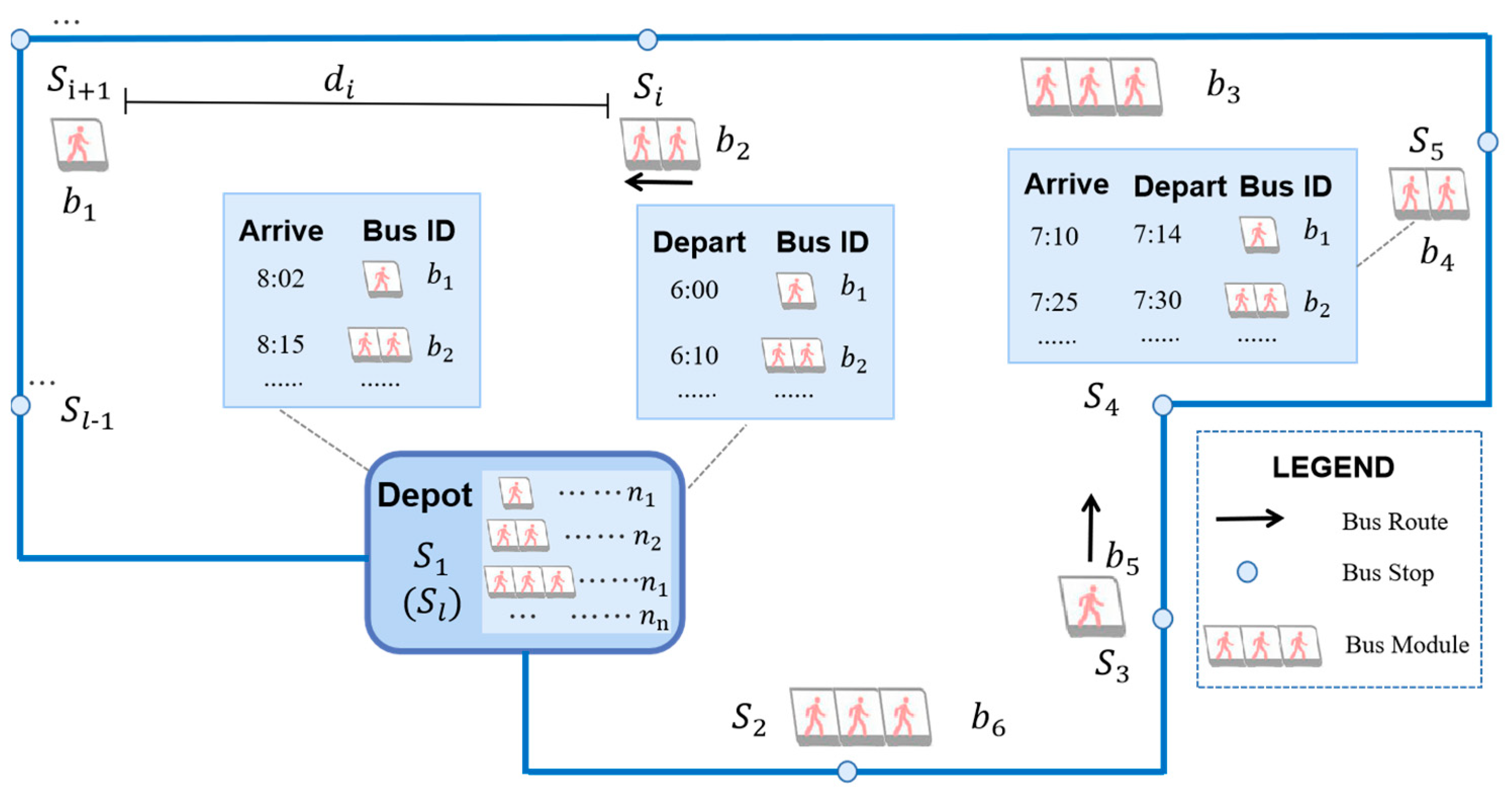
2. Problem Description

In this study, we examine a flexible modular intelligent connected bus system in the context of reservation scenarios. The multi-module bus fleet departs from the initial station S₁, travels along a fixed circular route to serve passengers, and eventually returns to the depot, as illustrated in Figure 1. For urban maneuverability, bus modules employ dynamic decoupling–reconnection strategies when negotiating turns: vehicle-to-vehicle (V2V) communication enables temporary separation to satisfy street curvature constraints, with millimeter-wave radar and LiDAR maintaining real-time kinematic alignment during turning maneuvers. At complex intersections, lead modules execute trajectory-splitting optimization and broadcast path data to followers via C-V2X technology, ensuring coordinated navigation through confined spaces. Multiple grouped bus units can be considered as a high-capacity bus. The bus’s capacity and operational costs vary based on the grouping of buses. Multi-module buses can pick up reserved passengers at all intermediate stations S_i. As shown in Figure 2, if there are no passengers boarding or alighting at a particular station, the bus may skip these stops. The dwell time at each station is determined by the boarding and alighting activities of passengers. The dwell-stop strategy used in the model is as follows: if the vehicle stops at a station, an additional stop time is set. If it does not stop, the $hol{d}_{i,j}$ at that station is set to 0.

To establish the mathematical model for the problem under study, we make the following assumptions, which are necessary to simplify the complex dynamics of bus scheduling while maintaining practical relevance and computational feasibility, with a focus on reservation-based modular bus systems and dynamic scheduling strategies as the core research objectives.

Assumption 1: The vehicle formation process is carried out exclusively at the starting station. Assumption 2: Vehicles maintain the departure sequence during operation, i.e., overtaking is not permitted. Assumption 3: Passengers at each station are served on a first-come, first-served basis. Delays for passengers may occur due to vehicle capacity constraints. Assumption 4: Consecutive buses cannot skip stations at the same stop, and a single bus cannot skip two or more stations consecutively. Assumption 5: Passengers who are waiting are allowed to board within the station dwell time.

3. Model Formulation

3.1. Notation

For the reader’s convenience, all symbols used in the equations are tabulated in

Table 1. Notation table.

Symbol	Description
Decision variable
$x_{m,k}$	decision variable: vehicle type m for departure at time k
$y_{i,j}$	decision variable: if vehicle i stops at station j, $y_{i,j}=1$, and 0 otherwise
Set	description
$K$	discretize the scheduling period into K uniformly distributed time intervals, and the discrete time nodes are given by $k\in K=\{0,1,\dots \dots n_k\}$
$S$	bus stops $j\in S=\left\{1,2,\dots \dots S\right\}$
$M$	fleet types of public buses $m\in M=\left\{1,2,\dots \dots m\right\}$
$i$	bus ID $i\in I=\left\{1,2,\dots \dots n\right\}$
$j$	bus stop ID
$P_j$	passenger requests at stop $j$
Parameters
$t_j$	travel time between stations $j~j-1$
$C_i$	capacity of the $i$-th bus
$C_r$	operational value of the vehicle
${\tau }_a$	time spent by a passenger boarding the bus/min
${\tau }_b$	time spent by a passenger disembarking/min
$C_a^F$	fixed operating costs of smart connected buses, including maintenance costs, per trip in CNY
$c$	capacity of the smart connected bus module
$C_a^V$	operational cost of the smart connected bus during operation, measured in CNY per trip
$2\mathsf{\delta }$	acceleration and deceleration time for vehicles entering and exiting the station
$a_{i,j}$	the time for vehicle i to arrive at station j
$d_{i,j}$	the time for vehicle i to depart at station $j$
$u_{i,j}$	the service time of vehicle i at station $j$
$H_{i,j}$	the headway between vehicle $i-1$ and i at station $j$
$h_0$	minimum headway
$D_{i,k}$	the number of passengers alighting from bus i at station $k$
$W_{i,j,k}$	passengers waiting at station $j$ for bus i bound for station $k$
$Au{p}_{i,j,k}^p$	passengers successfully boarding bus i heading to k in request p at station j
$D{o}_{i,j}$	passengers alighting from bus i at station j
$hol{d}_{i,j}$	dwell time of bus i at station j
$t_{j,k}^p$	the expected time for request p from station $s_b$ to $s_a$
$W{1}_{i,j}\left(h\right)$	passengers waiting for bus i at station j during time period h
$w_{i,j,k}^p$	passengers detained by bus i from station j to k for request p
${\beta }_{j,k}^p$	passengers from station j to k for request p
$a_{I,j}$	the last time i car was served before reaching j
$L_{i,j,k}$	passengers on i car going from j to k
$u{p}_{i,j}$	the actual number of passengers boarding i car at station j
$u{p}_{i,j}^H$	the number of passengers successfully boarding i car at station j who requested travel within the interval $[d_{I,j},a_{i,j}]$
$\tilde{t}$	the beginning of the planning horizon
${\varphi }_i$	discrete departure time nodes for vehicle i
${\theta }_{\mathrm{i}}$	vehicle types
$z_{p,i}$	passenger reservation request p is assigned to be served by vehicle i
${\zeta }_j^p$	${\zeta }_j^p=1$ indicates that the origin of passenger p is $S_j$
${\varrho }_j^p$	${\varrho }_j^p=1$ indicates that the destination of passenger p is $S_j$
$\widetilde{j_i}$	the index of the station where vehicle i is currently located or is about to arrive
$W_{skip}$	passengers delayed due to skip-stop
$Wait\_ski{p}_{i,j}$	the waiting time of passengers delayed because vehicle i skipped stop j
$w{s}_{i,j}^p$	overloaded passengers delayed within the service time
Wait_n1	passengers delayed due to bus capacity constraints arriving within the time range $[a_{i,j},a_{i,j}+hol{d}_{i,j}+u_{i,j}]$
$w{h}_{i,j}^p$	part of the passengers arriving within the dwell-stop time $hol{d}_{i,j}$ during the dwell time are delayed
Wait_n2	passengers arriving within the time range $[a_{i,j},a_{i,j}+hol{d}_{i,j}+u_{i,j}]$ are delayed due to bus capacity constraints

.

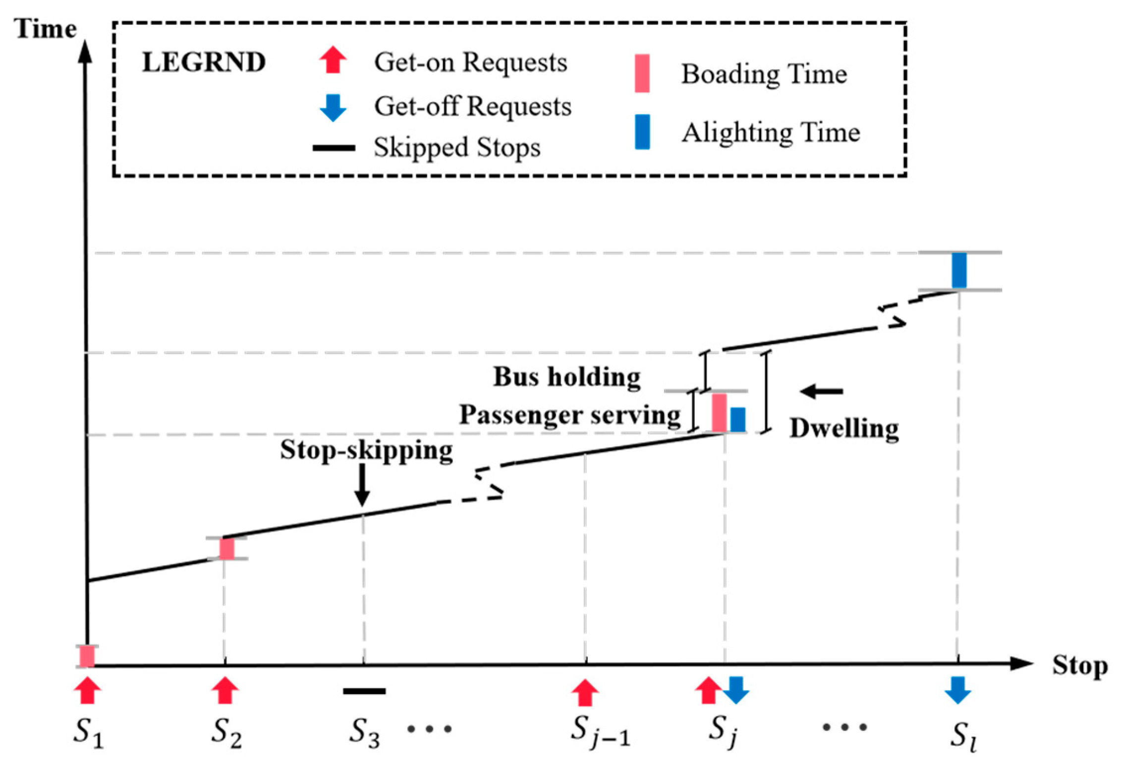
3.2. Passenger Boarding and Alighting Process State

The proposed two-level optimization model in this study primarily aims to determine two variables. One is the binary decision variable $x_{m,k}$, representing the dynamic grouping scheme of vehicles and departure time. Specifically, $x_{m,k}=1$ indicates dispatching an intelligent connected bus with a grouping length of $m$ at time node $k$; Otherwise, it indicates no dispatch. The other variable is the binary variable $y_{i,j}$ that determines whether bus $i$ will skips station $j$. If $y_{i,j}=0$, passengers waiting at station $j$ cannot board, and passengers destined for station $j$ on bus $i$ need to alight at station $j-1$. Simultaneously, to avoid impacting the operational efficiency of the bus, no station stop control is applied to bus $i$ that skips station $j$. Passengers can obtain information about skipped stations at each station through electronic signage. Suppose the passenger request count at station $j$ is $P_j$, and for each passenger $pϵP_j$, the request has origin–destination points $S_aϵS$, $S_bϵS$, and an expected boarding time $t_{j,k}^pϵ[0,T]$, where $j=S_a, k=S_b$. Therefore, we denote ($t_{j,k}^p,S_a,S_b$) as the request data for passenger $p$.

Firstly, the scheduling period $T$ is discretized into $K$ evenly distributed time intervals, where discrete time point $k\in K=\left\{0,1,\dots \dots k\right\}$, and the interval length is $\mathsf{\xi }=T/K$. The number of vehicles $n$ dispatched during operation can be represented as $n={\displaystyle {\displaystyle \sum }_{mϵM}}{\displaystyle {\displaystyle \sum }_{kϵK}}{x}_{m,k}$. Vehicles $i\in I=\{1,2\dots n\}$ operate sequentially, where $i=1$ is the first dispatched vehicle, and $i=n$ is the last dispatched vehicle. Based on the decision variables $x_{m,k}$, the departure time $d_{i1}$ and vehicle type ${\theta }_i$ of vehicle $i$ can be obtained as Equations (1)–(3), where ${\varphi }_i$ represents the discrete departure time node for vehicle $i$.

$$d_{i,1}=\mathsf{\xi }{\varphi }_i i\in I$$

(1)

$${\theta }_{\mathrm{i}}={\displaystyle \sum }_{m\in M}m{x}_{\mathrm{m},{\varphi }_i}$$

(2)

$${\varphi }_i={\displaystyle \sum }_{i\in I}{\displaystyle \sum }_{j\in S}{x}_{m,k}min\{k\mid {\displaystyle \sum }_{t⩽k}{\displaystyle \sum }_{m\in M}{x}_{mt}=i,k\in K\}$$

(3)

During the process of reaching subsequent station $j$, there is an acceleration and deceleration time of $2\delta$ when the vehicle enters and exits the station. The departure time of vehicle $i$ is the sum of the departure time from the previous station $d_{i,j-1}$, the inter-station travel time $t_j$, and the service time at station $j$, denoted as $u_{i,j}$.

$$a_{i,j}=d_{i,j-1}+\mathsf{\delta }{y}_{i,j-1}+t_j+\mathsf{\delta }{y}_{i,j}$$

(4)

$$d_{i,j}=a_{i,j}+u_{i,j}{y}_{i,j}+hol{d}_{i,j}{y}_{i,j}$$

(5)

For passenger request $p\in P$, corresponding bus service will be arranged, $z_{p,i}=1$. However, passenger request $p\in P$ cannot be assigned to bus trips that have already passed their originating stations, as shown in Equation (6).

$$\begin{array}{cc}{\displaystyle {\displaystyle \sum }_{i\in I}}{z}_{p,i}=1& \forall pϵP\end{array}$$

(6)

$$\begin{array}{cc}{z}_{p,i}\le 1-{{\displaystyle \sum }}_{j=1}^{\widetilde{j_i}-1}{\zeta }_j^p& \forall p\in P;i\in I\end{array}$$

(7)

For bus systems which use front and rear door boarding, passengers board and alight at the same time. Therefore, the passenger service time of the vehicle at the platform is taken as whichever is longest between the time taken for passengers to board and alight, as shown in Equation (9). Due to bus capacity constraints and the skip-stop strategy, there may be passengers waiting at station $j$ who cannot board vehicle $i$ currently serving at station $j$. Hence, it is necessary to estimate the number of passengers waiting at station $j$ and the number of passengers on the vehicle. This helps determine the number of waiting passengers during the service time and dwell time of vehicle $i$ at station $j$.

$$u_{i,j}=\max \{{\tau }_{a}u{p}_{i,j},{\tau }_{a}D{o}_{i,j}\left(\mathrm{t}\right)\}$$

(8)

$$\begin{array}{l}{W}_{i,j,k}=W{2}_{I,j}\left(H\right)+W{1}_{i,j}\left(h\right)+{\displaystyle {\displaystyle \sum }_{p\in P_{I,j}}}\left(1-y_{I,j+1}\right)W_{I,j,j+1}\\ +{\displaystyle {\displaystyle \sum }_{p\in P_{I,j}}}{{\displaystyle \sum }}_{k=j+1}^{\mathrm{s}}\left(1-y_{I,j}\right)W_{I,j,k}+{\displaystyle {\displaystyle \sum }_{p\in P_{I,j}}}{{\displaystyle \sum }}_{k=j+1}^s{w}_{I,j,k}^p\end{array}$$

(9)

where $W_{i,j,k}$ represents the total number of passengers with a planned origin at $j$ and destination at $k$ who are scheduled to be served by vehicle $i$, $W{2}_{I,j}\left(H\right)$ denotes the number of passengers who have arrived at station $j$ since the latest service by vehicle $I$, and $W{1}_{i,j}\left(h\right)$ represents the number of passengers arriving at station $j$ during the dwell time of vehicle $i$. $P_{i,j}$ represents the set of passenger requests at station $j$ that are assigned to vehicle $i$. The term $\left(1-y_{I,j+1}\right)W_{I,j,j+1}$ represents passengers waiting for vehicle $I$, who are detained at station $j$ due to the skipping of station $j+1$ by vehicle $I$. The expression ${\displaystyle {\displaystyle \sum }_{p\in P_{I,j}}}{{\displaystyle \sum }}_{k=j+1}^{\mathrm{s}}\left(1-y_{I,j}\right)W_{I,j,k}$ indicates the total number of passengers detained due to the skipping of station $j$ by vehicle $I$. Additionally, ${\displaystyle {\displaystyle \sum }_{p\in P_{I,j}}}{{\displaystyle \sum }}_{k=j+1}^s{w}_{I,j,k}^p$ represents passengers detained at station $j$ due to the capacity constraints of vehicle $I$.

$$W{2}_{I,j}\left(H\right)={\displaystyle {\displaystyle \sum }_{p\in P_{i,j}}}{{\displaystyle \sum }}_{k=j+1}^{\mathrm{s}}{\beta }_{j,k}^p$$

(10)

$P_{i,j}$ represents the set of passengers requesting travel within the time range $[d_{I,j},a_{i,j}]$.

$$W{1}_{i,j}\left(h\right)={\displaystyle {\displaystyle \sum }_{p\in P_{i,j}}}{{\displaystyle \sum }}_{k=j+1}^{\mathrm{s}}{\beta }_{j,k}^p$$

(11)

$P_{i,j}$ represents the set of passengers requesting travel within the time range [$a_{i,j},a_{i,j}+hol{d}_{i,j}+u_{i,j}$].

The waiting time for passengers at each station is categorized as follows:

(1)

Passengers stranded due to station skipping

The passengers stranded at station j due to station skipping can be divided into two situations: one takes place when bus i skips station j, whereby passengers requesting travel within the time range of the departure time of bus I’s $d_{I,j}$ and the arrival time of bus i’s $a_{i,j}$ cannot board bus i and need to wait for the arrival of bus i + 1; the other takes place when bus i skips station j + 1 and passengers waiting at station j with destination j + 1 cannot board bus i. The formula for calculating the number of passengers $W_{skip}$ stranded by bus i skipping stations at station j is given by Equation (12), and the corresponding waiting time for the stranded passengers is denoted as $Wait\_ski{p}_{i,j}$:

$$W_{skip}=\left\{\begin{array}{l}\begin{array}{ll}{\displaystyle \sum _{p\in P_j}{\displaystyle \sum _{k=j+1}^{\mathrm{s}}(1-y_{i,j})}}\times W_{i,j,k}& \mathrm{if}{y}_{i,j}=0\end{array}\hfill \\ \begin{array}{ll}(1-y_{i,j+1})Wi,j,k& \hspace{1em}\hspace{1em}\mathrm{if}{y}_{i,j+1}=0,y_{i,j}=1\end{array}\hfill \\ \begin{array}{ll}0& \hspace{1em}\hspace{1em}\hspace{1em}\hspace{1em}\hspace{1em}\hspace{1em}\hspace{1em}\mathrm{if}{y}_{i,j+1}=1,y_{i,j}=1\end{array}\hfill \end{array}\right.$$

(12)

$$Wait\_ski{p}_{i,j}=\left\{\begin{array}{l}\begin{array}{ll}{\displaystyle \sum _{p\in P_{i,j}}{\displaystyle \sum _{k=j+1}^{\mathrm{s}}(1-y_{i,j})}}{W}_{i,j,k}\times (a_{i+1,j}-d_{i,j})& \mathrm{if}{y}_{i,j}=0\end{array}\hfill \\ \begin{array}{l}{y}_{i+1,j}(1-y_{i,j+1})W_{i,j,j+1}\times (a_{i+1,j}-d_{i,j})+y_{i+2,j+1}(1-y_{i+1,j})(1-y_{i,j+1})W_{i,j,j+1}\times (a_{i+2,j}-d_{i,j})\\ \hspace{1em}\hspace{1em}\hspace{1em}\hspace{1em}\hspace{1em}\hspace{1em}\hspace{1em}\hspace{1em}\hspace{1em}\hspace{1em}\hspace{1em}\hspace{1em}\hspace{1em}\hspace{1em}\mathrm{if}{y}_{i,j+1}=0,y_{i,j}=1,y_{i+2,j+1}=1\end{array}\hfill \\ \begin{array}{ll}0& \hspace{1em}\hspace{1em}\hspace{1em}\hspace{1em}\hspace{1em}\hspace{1em}\hspace{1em}\hspace{1em}\hspace{1em}\hspace{1em}\hspace{1em}\hspace{1em}\mathrm{if}{y}_{i,j+1}=0 ,y_{i,j}=1\end{array}\hfill \end{array}\right.$$

(13)

The term vehicle $I$ refers to the identification number of the bus that last provided passenger service at the station. In this context, vehicle $i+1$ is not strictly considered as the next vehicle in line, but rather the next bus available to serve stranded passengers.

(2)

Passengers stranded due to bus capacity limitations

When bus i passes through station j, the total number of passengers on the bus, including waiting passengers at station j, may exceed bus i’s capacity, $W{2}_{I,j}\left(H\right)-D{o}_{i,j}\left(t\right)+L_{i,j-1}\ge C_i$. Then, the stranded passengers will have to wait for the arrival of bus $i+1$. Under the control of the dwell-time strategy, the bus needs to wait for a certain period after passengers complete boarding and alighting. Overloading occurs during bus $i$’s service time $u_{i,j}$ and dwell-time $holdin{g}_{i,j}$. Therefore, the total number of passengers stranded due to bus capacity limitations $w_{i,j}^p$ can be calculated by Equation (14), and the total waiting time $Wait\_n$ for this group of stranded passengers can be calculated by Equation (15).

$$w_{i,j}^p=w{s}_{i,j}^p+w{h}_{i,j}^p$$

(14)

$$Wait\_n=Wait\_n1+Wait\_n2$$

(15)

(a)

Overloading occurs during the service time

When overloading occurs during the service time, only a few passengers requesting travel within the time range $[d_{I,j},a_{i,j}]$ can board, while the remaining passengers and those waiting during the waiting time $[a_{i,j},a_{i,j}+hol{d}_{i,j}+u_{i,j}]$ are detained. The number of detained passengers, denoted as $w{s}_{i,j}^p$, is calculated as shown in Equation (16).

$$w{s}_{i,j}^p={\displaystyle \sum }_{k=j+1}^{\mathrm{s}}w{s}_{i,j,k}^p=\left\{\begin{array}{l}\begin{array}{l}W{2}_{I,j}\left(H\right)-C_i+L_{i,j-1}-D{o}_{i,j}+W{1}_{i,j}\left(h\right)\hfill \\ \hspace{1em}\hspace{1em}\mathrm{if}W{2}_{I,j}\left(H\right)-D{o}_{i,j}+L_{i,j-1}\ge C_i,y_{i,j}=1\hfill \end{array}\hfill \\ \begin{array}{cc}0& \hspace{1em}\mathrm{otherwise}\end{array}\hfill \end{array}\right.$$

(16)

The waiting time for these passengers includes the stopping time of bus $i$ and the interval time between the arrival of buses $i$ and $i+1$ at station $j$. Therefore, the waiting time for this portion of detained passengers is calculated as shown in Equation (17).

$$Wait\_n1=\left\{\begin{array}{l}\begin{array}{l}(W{2}_{I,j}(H)-C_i+L_{i,j-1}-D{o}_{i,j})\times [hol{d}_{i,j}+(a_{i+1j}-d_{i,j})]+W{1}_{i,j}\left(h\right)\\ \times [{\displaystyle \frac{1}{2}}hol{d}_{i,j}+(a_{i+1,j}-d_{i,j})]\hspace{1em}\hspace{1em}\hspace{1em}\mathrm{if}W{2}_{I,j}(H)-D{o}_{i,j}+L_{i,j-1}\ge Ci,y_{i,j}=1\end{array}\hfill \\ \begin{array}{cc}0& \hspace{1em}\hspace{1em}\hspace{1em}\hspace{1em}\hspace{1em}\hspace{1em}\hspace{1em}\hspace{1em}\hspace{1em}\hspace{1em}\hspace{1em}\mathrm{otherwise}\end{array}\hfill \end{array}\right.$$

(17)

• (b) Overloading occurs during the dwell-stop time

When overloading occurs during the dwell-stop time, passengers within the time interval $[a_{i,j},a_{i,j}+hol{d}_{i,j}+u_{i,j}]$ can board the bus, while the portion of passengers arriving within the dwell-stop time period $hol{d}_{i,j}$ denoted as $w{h}_{i,j}^p$ will be detained, calculated as in Equation (18).

$$w{h}_{i,j}^p={\displaystyle \sum _{k=j+1}^{\mathrm{s}}w}{h}_{i,j,k}^p=\left\{\begin{array}{l}\begin{array}{l}W{2}_{l,j}(\mathrm{H})-C_i+L_{i,j-1}-D{o}_{i,j}+W{1}_{i,j}\left(h\right)\\ \mathrm{if}W{2}_{I,j}\left(H\right)+W{1}_{i,j}(h)-D{o}_{i,j}+L_{i,j-1}\ge C_i\ge W{2}_{I,j}(H)-D{o}_{i,j}+L_{i,j-1},y_{i,j}=1\end{array}\hfill \\ \begin{array}{cc}0& \mathrm{otherwise}\end{array}\hfill \end{array}\right.$$

(18)

The waiting time for these passengers includes the dwell time of bus $i$ and the interval time between the arrivals of buses $i$ and $i+1$ at station $j$. Therefore, the waiting time for this portion of detained passengers is calculated as in Equation (19).

$$Wait\_n2=\left\{\begin{array}{c}\begin{array}{l}w{h}_{i,j}^p\{{\displaystyle \frac{1}{2}}hol{d}_{i,j}-(W{2}_{I,j}(\mathrm{H})-C_i+L_{i,j-1}-D{o}_{i,j}+W{1}_{i,j}(\mathrm{h}))\times {\displaystyle \frac{hol{d}_{i,j}}{W{1}_{i,j}(\mathrm{h})}}]+(a_{i+1,j}-d_{i,j})\}\\ \mathrm{if}W{2}_{I,j}(\mathrm{H})+{\mathrm{W}1}_{i,j}(\mathrm{h})-D{o}_{i,j}+L_{i,j-1}\ge {\mathrm{C}}_i\ge \mathrm{W}{2}_{I,j}(\mathrm{H})-D{o}_{i,j}+L_{i,j-1},y_{i,j}=1\end{array}\\ \begin{array}{cc}0& \mathrm{otherwise}\end{array}\end{array}\right.$$

(19)

The calculation of passenger-related variables in the above formulas is as follows:

$$L_{i,k}={\displaystyle \sum }_{j=1}^k\left(u{p}_{i,j}-D{o}_{i,j}\right)$$

(20)

$$D_{i,k}={{\displaystyle \sum }}_{j=1}^{k-1}{y}_{i,j}\times L_{i,k}$$

(21)

$$u{p}_{i,j}=\left\{\begin{array}{ll}0\hfill & \mathrm{if}{y}_{i,j}=0\\ C_i+D{o}_{i,j}-L_{i.j-1}\hfill & \mathrm{if}W{2}_{I,j}\left(\mathrm{H}\right)+W{1}_{i,j}\left(\mathrm{h}\right)-D{o}_{i,j}+L_{i,j-1}\ge C_i,y_{i,j}=1\\ W_{i,j,k}\hfill & \mathrm{otherwise}\end{array}\right.$$

(22)

$$D{o}_{i,j}=y_{i,j}\left[D_{i,j}+\left(1-y_{i,j+1}\right)D_{i,j+1}\right]$$

(23)

$$u{p}_{i,j}^H=\left\{\begin{array}{l}\begin{array}{cc}0& \hspace{1em}\hspace{1em}\hspace{1em}\hspace{1em}\hspace{1em}\mathrm{if}{y}_{i,j}=0\end{array}\hfill \\ \begin{array}{cc}{C}_i+D{o}_{i,j}-L_{i,j-1}& \mathrm{if}W{2}_{I,j}(H)-D{o}_{i,j}+L_{i,j-1}\ge C_i,y_{i,j}=1\end{array}\hfill \\ \begin{array}{cc}W{2}_{I,j}(H)+(1-y_{I,j+1})W_{I,j,j+1}+{\displaystyle \sum _{p\in P_{I,j}}{\Sigma }_{k=j+1}^{\mathrm{s}}}(1-y_{l,j})W_{l,j,k}+{\displaystyle \sum _{p\in P_{I,j}}{\displaystyle \sum _{k=j+1}^s{w}_{I,j,k}^p}}& \mathrm{otherwise}\end{array}\hfill \end{array}\right.$$

(24)

$$w_{i,j,k}^p=W_{i,j,k}-Au{p}_{i,j,k}^p$$

(25)

The calculation of the total waiting time for passengers is as follows:

$$W_{wait}={\displaystyle \sum }_{i\in V}{\displaystyle \sum }_{j\in S}{\displaystyle \sum }_{p\in P_j}\{{\displaystyle \sum }_{k=j+1}^{\mathrm{S}}\left[\left(a_{i,j}-t_{j,k}^p\right)\right]+Wait\_skip+Wait\_n\}$$

(26)

The calculation of the travel time for passengers is as shown in Equation (27):

$$W_{travel}={\displaystyle \sum }_{i\in V}{\displaystyle \sum }_{j\in S}{\displaystyle \sum }_{p\in P_j}\left[L_{i,j-1}\times \left(\mathsf{\delta }{y}_{i,j-1}+u_{i,j}+\mathsf{\delta }{y}_{i,j}\right)\right]+T_{i,j}^{ON}\times y_{i,j}$$

(27)

$T_{i,j}^{ON}$ represents the time that bus $i$ waits for passengers to board and alight at station $j$, and the calculation formula is as shown in Equation (28):

$$T_{i,j}^{ON}=\left\{\begin{array}{l}\begin{array}{l}\begin{array}{cc}(L_{i,j-1}+u{p}_{i,j}^H+D{o}_{i,j})\times (u_{i,j}+hol{d}_{i,j})+W{1}_{i,j}(h)\times {\displaystyle \frac{hol{d}_{i,j}}{2}}& \mathrm{if}{L}_{i,j}\le C_i\end{array}\\ \begin{array}{cc}{L}_{i,j}(u_{i,j}+hol{d}_{i,j})& \hspace{1em}\hspace{1em}\hspace{1em}\hspace{1em}\hspace{1em}\hspace{1em}\hspace{1em}\mathrm{if} L_{i,j-1}+W{2}_{I,j}(H)-D{o}_{i,j}\ge C_i\end{array}\end{array}\hfill \\ (L_{i,j-1}+u{p}_{i,j}^H+D{o}_{i,j})\times (u_{i,j}+hol{d}_{i,j})+({\mathrm{L}}_{\mathrm{i},j}-u{p}_{i,j}^H)\times [hol{d}_{i,j}-{\displaystyle \frac{1}{2}}(u{p}_{i,j}-u{p}_{i,j}^H)\times {\displaystyle \frac{hol{d}_{i-1,j}}{W{1}_{i-1,j}(\mathrm{h})}}\hfill \\ \mathrm{if}W{2}_{I,j}(\mathrm{H})+W{1}_{i,j}(\mathrm{h})-D{o}_{i,j}+L_{i,j-1}\ge C_i\ge W{2}_{I,j}(\mathrm{H})-D{o}_{i,j}+L_{i,j-1}\hfill \end{array}\right.$$

(28)

The cost of the bus operation process, denoted as $Car\_run$, is calculated using Equation (29):

$$Car\_run={\displaystyle \sum }_{i\in V}{\displaystyle \sum }_{j\in S}\left\{C_r\left[\mathsf{\delta }{y}_{i,j-1}+t_{i,j}+\mathsf{\delta }{y}_{i,j}+\left(u_{i,j}+hol{d}_{i,j}\right)\times y_{i,j}\right]\right\}$$

(29)

The cost incurred by bus departure, denoted as $f_m$, is calculated using Equation (30):

$$f_m=\begin{array}{cc}{C}_a^F+C_a^{V}m& m=1\dots A\end{array}$$

(30)

3.3. Constraints

The constraint (33) prohibits consecutive station skipping for the same bus, meaning that a bus is not allowed to skip two consecutive stations. Therefore, if a bus skips station $j$, it must serve station $j+1$. Constraint (34) prohibits consecutive station skipping for two consecutive buses. In other words, if bus $i$ skips station $j$, bus $i+1$ must serve that station. Constraint (35) ensures the service quality of scheduled buses, whereby the total number of passengers on each vehicle must not exceed the bus’s capacity limit $C_i$. This constraint helps guarantee passenger comfort and safety while also mitigating the risk of overcrowding.

$$d_{i,1}-d_{i-1,1}\ge h_0$$

(31)

$$d_{i,j}\ge d_{i-1,j}$$

(32)

$$\begin{array}{ccc}{y}_{i,j}+y_{i,j+1}\ge 1& j=1,2,\dots s& \forall i\end{array}$$

(33)

$$\begin{array}{ccc}{y}_{i,j}+y_{i+1,j}\ge 1& i=1,2,\dots n-1& \forall j\end{array}$$

(34)

$$u{p}_{i,j}+L_{i,j-1}-D{o}_{i,j}\le C_i$$

(35)

3.4. Objective Function

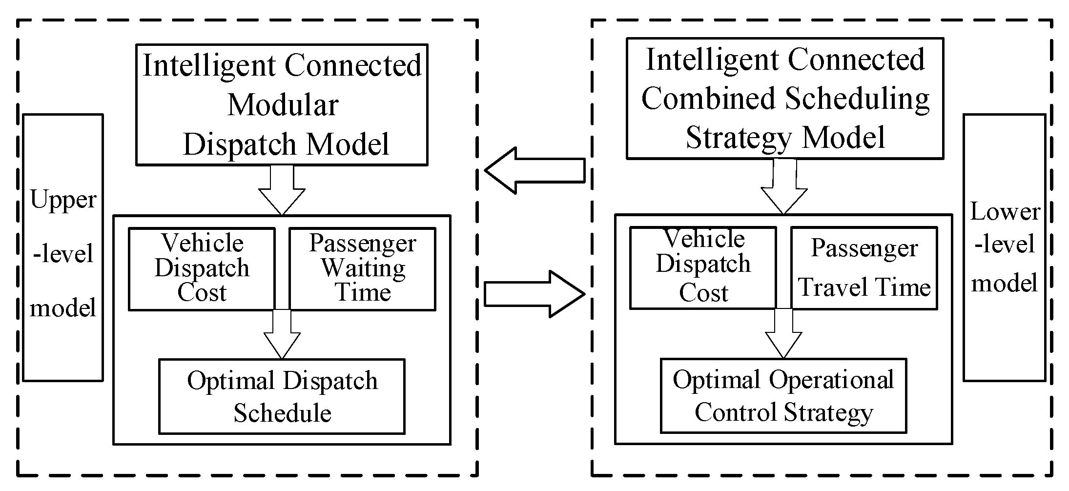
The upper- and lower-level models are related through a dominance relationship. The bi-level planning model prioritizes the selection of high-quality vehicle grouping and departure time schemes based on the upper-level model, aiming to maximize passenger service and public transportation operational profit. Subsequently, the selected departure scheme is optimized with skip-stop strategies at each station within the lower-level model. After establishing the spatiotemporal relationships for each bus and passenger, the following bi-level model can be proposed:

(1)

Upper-level model

The upper-level model aims to generate the optimal departure plan, with the decision variables being the size of the vehicle grouping and the departure times. It optimizes the bus schedule timetable (including departure time, station stop time, station-to-departure time), the dynamic departure grouping scheme, and the vehicle-matching scheme. The objective is to minimize both vehicle travel time and passenger waiting time. The specific formula is as follows:

$$\min z_1=w_1\times Ca{r}_{run}+w_2\times W_{wait}\times b_1$$

(36)

(2)

Lower-level model

The lower-level model aims to generate the optimal operational control strategy, specifically the skip-stop strategy, which minimizes both vehicle travel time and passenger waiting and travel time. The specific formulas are as follows:

$$\left\{\begin{array}{c}\min z_2=Ca{r}_{run}\\ \min z_3=W_{travel}\end{array}\right.$$

(37)

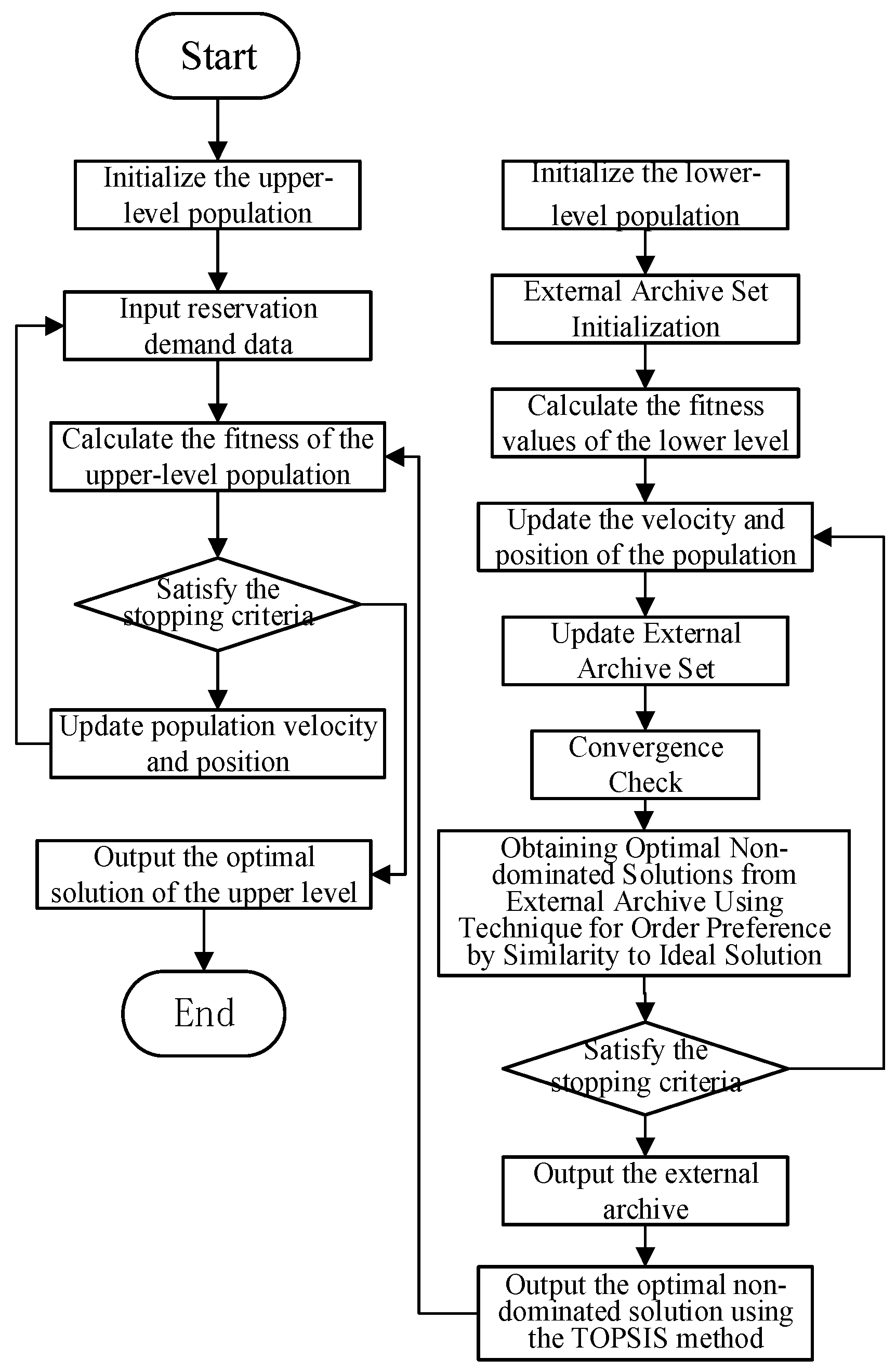
4. Solution Algorithm

We constructed a dual-layer optimization model for bus scheduling based on the reservation scenario, comprehensively considering skip-stop and dwell-stop strategies. During the solution process, parameters are exchanged between the upper and lower layers. The lower layer’s optimization problem involves multi-objective optimization. To select the optimal solution from the Pareto non-dominated solution set, meticulous analysis and comparison through an evaluation model are required. As illustrated in Figure 3, in our dual-layer optimization model, the upper layer’s decision variables $x_{m,k}$ determine the size of the grouped vehicles and departure times, while the lower layer’s decision variables $y_{i,j}$ determine the stopping arrangements of each bus at each station. The upper-layer model is solved by transforming into a single-objective problem through weighted conversion. The lower-layer model employs a multi-objective optimization algorithm based on the grid vector pruning strategy according to the ${\delta }_k$–dominance relationship [17]. This algorithm effectively avoids population degeneration issues, significantly enhancing convergence performance and maintaining good solution diversity during the optimization process [17].

However, parameter setting in this method requires manual intervention, posing a challenge in its determination. Therefore, an improved particle swarm optimization algorithm based on T-DLPSO-TOPSIS (Two-Layered Dynamic Multi-Objective Particle Swarm Optimization with Technique for Order of Preference by Similarity to Ideal Solution) is proposed here for model solution. The main principles of this algorithm are summarized as follows:

(1)

Population particle velocity and position component update.

(2)

Parameter ${\delta }_k$ and adaptive adjustment

In the context of minimizing a multi-objective optimization problem, setting particle $n_1$’s parameter ${\delta }_k$ dominates over $n_2$, expressed mathematically as follows:

$$f_k\left(n_1\right)-{\delta }_k\le f_k\left(n_2\right) \forall k\in \left[1,2,\dots ,K\right]$$

(38)

$f_k\left(n\right)$ represents the value of objective $k$ for particle $n$; ${\delta }_k$ is the parameter for objective $k$; and $K$ is the number of objectives.

The current optimal solution generated during each iteration update is saved to a specific collection, namely the external repository. ${\delta }_k$ is influenced by the external repository, and the adjustment strategy is as follows:

$${\delta }_k={\displaystyle \frac{f_k^{max}-f_k^{min}}{M}}$$

(39)

where $f_k^{max}$ and $f_k^{min}$ represent the maximum and minimum values of objective function $k$, respectively, and $M$ is the capacity of the external repository.

(3)

External repository grid update

Define a $K$-dimensional objective space and divide it into $N_1\times N_2\times \dots \times N_K$ grids, with the vector belonging to each grid given by Equation (40):

$${\beta }_k\left(n\right)=\left[{\displaystyle \frac{f_k\left(n\right)-f_k^{min}}{{\delta }_k}}\right]$$

(40)

where [] denotes the floor function.

Add the updated particle to the external archive, and update the grid according to the following strategy:

(a)

Remove the examples that exceed the extremes of their respective objective functions.

(b)

If a grid contains only one particle, it is retained directly.

(c)

If a grid contains the extreme values of objective K, all other particles in this grid are removed, and only the extreme points are retained.

(d)

If a grid contains multiple particles and no extreme points, the distances D(n) between each particle and the grid vector are compared, and the particle with the minimum distance is retained, as expressed in Equation (41).

$$D(n)=\sqrt{\sum _{k=1}^K{\left[{\displaystyle \frac{f_k(n)-f_k^{\min }}{{\delta }_k}}-{\beta }_k(n)\right]}^2}$$

(41)

(e)

Selection of $P_{best}$ and $g_{best}$

Selection of $P_{best}$: Compare the particle after iteration with its $P_{best}$ and choose the dominating one between them.

Selection of $g_{best}$: In the external storage set, choose the particle with the smallest angle, with the particle as its $g_{best}$.

The solution steps for the dual-layer model are outlined in Figure 4.

5. Numerical Experiments

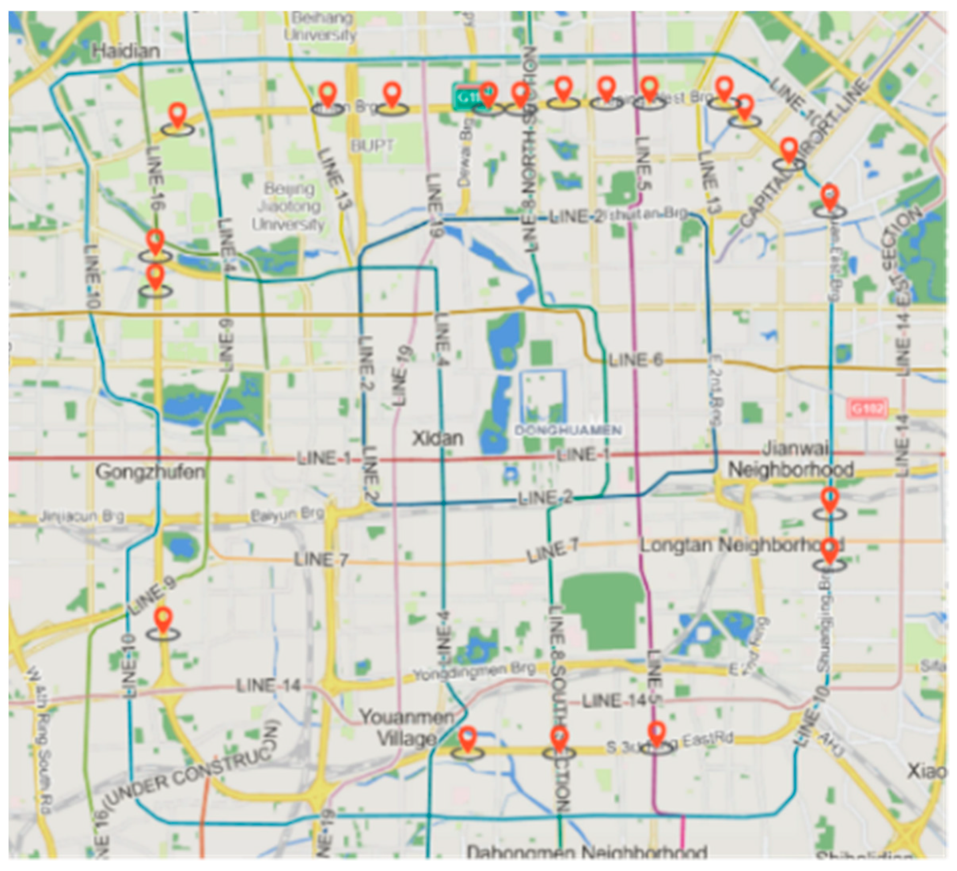
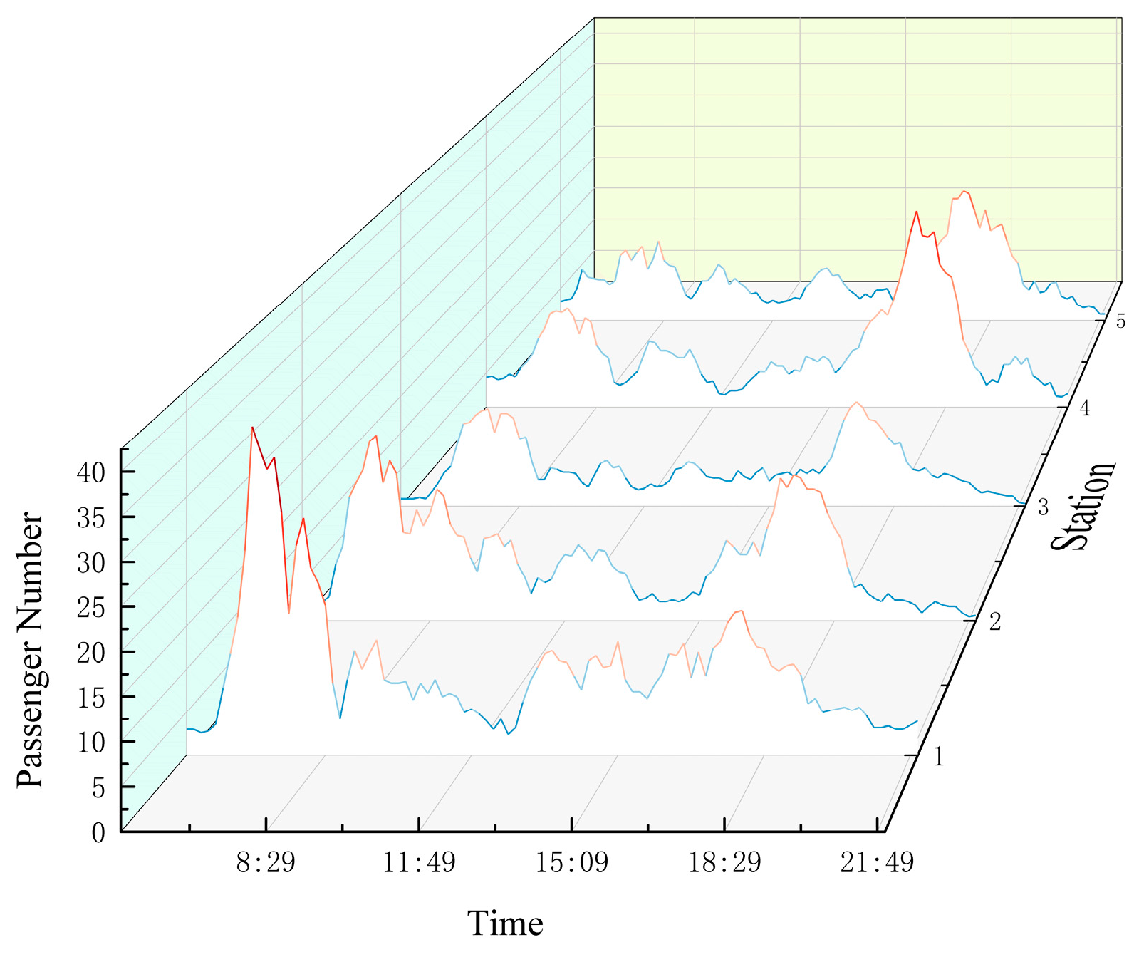
5.1. Data Analysis

Numerical experiments were conducted based on the inner loop of Bus Route 300 in Beijing, which is a circular route consisting of 35 stations with a total length of approximately 47.5 km, as shown in Figure 5. The demand data for reserved passengers were extracted from actual bus card-swiping data for Bus Route 300. The original data covered the time range of 1 December 2021, from 5:00 to 22:00. It included information on passenger origin and destination stations, boarding and alighting card-swiping times, and vehicle identification numbers.

IC card data were utilized to generate reservation passenger demand data. First, based on actual passenger swipe data, we estimated the passenger arrival intensity at each bus stop, employing a non-homogeneous Poisson process to capture the time-varying characteristics of passenger arrivals [29]. The swipe data underwent preprocessing, including the removal of null and duplicate records, as well as the identification and handling of outliers. The processed data were then used to calculate the departure times of each bus at every station and the number of passengers boarding at each stop, enabling the estimation of passenger arrival intensity at different time intervals.

Continuously repeating this process, we obtained the passenger arrival intensity curves for each station of Beijing’s 300 inner-ring bus on 1 December 2021. Conducting statistical analyses on passenger travel from both temporal and spatial dimensions, Figure 6 illustrates the variations in passenger travel at each station over a 24 h period. It can be observed that the distribution of passenger travel times exhibits distinct peak periods in the morning and evening. Peak travel times are concentrated between 6:00 and 9:00 in the morning and 17:00 and 19:00 in the evening. This pronounced peak phenomenon aligns with the commuting behavior of passengers on workdays. Based on the characteristics of passenger travel behavior, it can be inferred that the demand for scheduled buses is suitable for morning peak travel, and individuals traveling during this period can be considered potential users of scheduled buses.

To further extract demand data for scheduled bus passengers, this study compared and analyzed the waiting and travel times of regular and scheduled buses spatially to explore the advantages of scheduled bus services. Traditional methods of obtaining waiting times for regular bus passengers, such as questionnaire surveys and video collection [29], are time-consuming and limited to short-term observations at typical stations, unable to capture the average waiting times per passenger at the route or network level. Here, this study calculated multi-scale passenger waiting times based on non-homogeneous Poisson distribution. By integrating the obtained passenger arrival intensity at each station with the departure times of buses, the expected average waiting time for passengers at any given time and spatial scale was obtained. This allowed us to determine the actual waiting time corresponding to the observed travel data. Combining this with the boarding and alighting times, we could calculate the total travel time for actual passengers.

The comparative results of total travel time for passenger trips under optimized dispatching scenarios—both for conventional buses and the proposed scheduled reservation-based bus system—are illustrated in Figure 7. The blue dots represent travel times for regular buses, while the red dots correspond to the reservation-based system. Key observations include the following:

Short-distance trips (≤10 km): The travel times for both systems overlap significantly, indicating a minimal advantage of reservation-based buses in this range.

Long-distance trips (>10 km): The reservation-based system demonstrates stable and reduced travel times compared to conventional buses, with the gap widening notably for trips exceeding 20 km. This aligns with the system’s optimization logic, which prioritizes demand-responsive scheduling for longer commutes.

Data selection rationale: To focus on peak-hour efficiency, this study analyzed 1865 passengers with travel distances >10 km, as the reservation-based system began to demonstrate measurable time-saving advantages in this range.

5.2. Model Validation

In this section, the paper considers the demand for scheduled passengers during the peak hours of December 1st on the Beijing City Bus Route 300’s inner ring. The travel time between route stations, denoted as $t_j$, was determined based on actual route operation times obtained from Gao De Map. The route provides modular bus unit services, where buses are composed of modular units which can be connected and detached at the starting point. Following the information provided by [17], this study assumed that a maximum of three bus units could be deployed, each with a capacity of 20 passengers. Consequently, three types of buses, denoted as $M=\left\{1,2,3\right\}$, were considered, with each type having a capacity of 20, 40, and 60 passengers, respectively.

This study evaluated the model based on bus type and scheduling strategy (skip-stop, dwell-stop).

Table 2. Simulation results for different scenarios.

Scenarios	Passenger Waiting Time		Passenger Travel Time		Operation Cost	Bus Operating Cost	Passengers’ Travel Cost	Total Cost
	Value/min	Variation/%	Value/min	Variation/%	Value/CNY	Value/CNY	Value/CNY	Value/CNY
1	9386.94	─	82,292.00	─	9408	─	80,858.96	─
2	7096.33	24.40	72,067.33	12.42	12,768	9789.40	69,406.97	91,964.37
3	6257.40	33.34	71,863.29	12.55	8383	8072.78	68,186.91	84,642.69
4	6163.82	34.34	71,789.22	12.76	8651	9083.9	68,007.72	85,742.62
5	5662.77	39.67	70,405.73	14.44	11,635	10,772	66,219.27	88,626.27
6	13,701.22	−45.96	69,956.08	14.99	6534	7592.6	75,889.64	90,016.24
7	5257.12	44.00	71,304.80	13.35	8976	9050.8	66,467.43	84,494.23

details the settings for all scenarios. Our modular bus scheduling considered a maximum of three bus modules, allowing for scenarios of no dispatch or dispatching single-, double-, or triple-module buses. Additionally, we explored a scenario with a maximum of four bus modules and studied the scheduling when conventional fixed-capacity buses were used in our appointment-based travel bus scheduling.

The scenarios were as follows: Scenario 1, conventional bus operation, serving as the baseline; Scenario 2, proposed scheduled travel bus scheduling with fixed-capacity buses; Scenario 3, modular intelligent connected bus scheduling for scheduled travel; Scenario 4, modular intelligent connected bus scheduling for scheduled travel with dwell-stop control only; Scenario 5, modular intelligent connected bus scheduling for scheduled travel with skip-stop control only; Scenario 6, maximum of four modular bus modules for scheduled travel; and Scenario 7, modular intelligent connected bus scheduling for scheduled travel, combining skip-stop and dwell-stop control strategies.

5.3. Results and Discussion

For each scenario, we conducted 10 simulations to ensure result stability. Each simulation had a duration of approximately 1.5 h. During each simulation run, the model generated outputs including bus trajectories, load factors, arrival and departure times, passenger boarding and alighting times, various cost components (operational and passenger costs), and detailed information on optimal scheduling decisions. Performance metrics such as average passenger waiting time, average bus occupancy, average bus speed, and headway variation were computed based on these outputs. All performance metrics were averaged over all simulation runs to eliminate randomness.

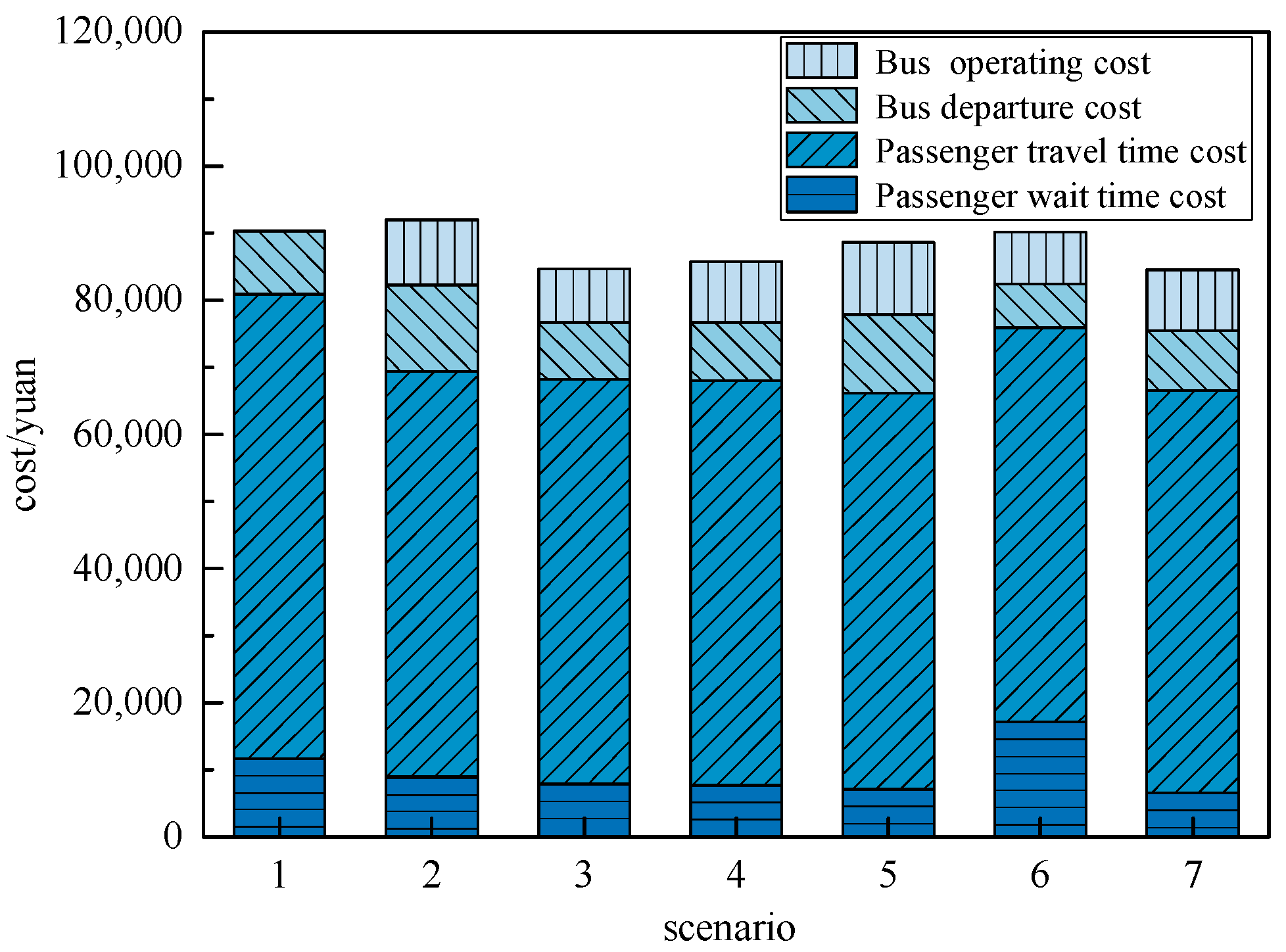
5.3.1. Cost and Time Characteristics of the Use of Various Scenarios

The scatter plots in Figure 8, Figure 9 and Figure 10 provide a visual comparison of passenger waiting time, journey time, and total journey time for Scenarios 1, 2, 3, 4, 5, 6, and 7. These plots not only illustrate the impact of different scheduling schemes on the passenger travel experience but also highlight the significant advantages of the proposed modular, intelligent, networked bus scheduling system for scheduled services outlined in this chapter. They provide compelling data support for the optimization of bus scheduling strategies.

Primarily from the perspective of passenger waiting time analysis, Figure 8 demonstrates the ability of the travel mode scheduling system outlined in this chapter to significantly reduce passenger waiting time. Compared to conventional bus systems, this system effectively keeps passenger waiting time within a stable range of less than 4 min, which is of paramount importance in improving passenger travel satisfaction and efficiency. Secondly, when comparing the scheduling effects under different modular unit number settings, it is noticeable that setting the maximum modular bus unit number to four yields inferior results compared to the scenario where it is set to three. This discrepancy is mainly attributed to the increase in decision variable dimensions, which leads to an exponential increase in computational complexity. Within the same optimization timeframe, the model struggles to identify the global optimum, further confirming the principle that a larger number of modules does not necessarily guarantee superior results. Therefore, in practical applications, the number of modules should be set according to specific scenarios and requirements to achieve a balance between efficiency and effectiveness. Through judicious modular configuration, the performance of this travel mode planning system can be further enhanced, providing passengers with more efficient and convenient travel services.

Furthermore, by comparing Scenarios 3, 4, 5, and 7, the impact of the skip-stop and dwell-stop control strategies on passenger travel time can be observed. Combining the data presented in the table, the implementation of the skip-stop strategy results in a reduction in passenger waiting time by 9.5% and a decrease in passenger travel time by 2.03%, demonstrating the effectiveness of the skip-stop strategy in enhancing public transit operational efficiency. With the introduction of the dwell-stop strategy, passenger waiting time is reduced by 1.5%, with minimal change in passenger travel time. When both skip-stop and dwell-stop strategies are implemented together, passenger waiting time is reduced by 15.99%, with some improvement in passenger travel time. This highlights the superior overall effects of a judicious combination of scheduling strategies in improving the operational efficiency of public transport. Figure 10 shows that the proposed system has certain advantages in passenger travel time over different travel distances. However, it is noteworthy that, in Scenario 7, where the dwell-stop strategy was implemented, passenger travel time was slightly increased compared to Scenario 5, in which no dwell-stop measures were taken. Therefore, while the dwell-stop strategy reduces waiting time, it may also lead to some increases in travel time, requiring a careful balance based on specific needs in practice.

To gain a deeper understanding of the relative merits and demerits of scheduling schemes across different scenarios, it is necessary to categorize passenger travel distances. For each distance interval, the travel and waiting times of passengers should be statistically analyzed. Based on the analysis presented in Figure 11, conclusions can be drawn: In terms of passenger travel time, the advantages of employing skip-stop and dwell-stop control strategies, as well as modular bus models, are not particularly pronounced when passengers travel short distances. This may be attributed to the relatively minor impact of vehicle operational efficiency and stopping points on travel time during short-distance trips, making it difficult to discern differences among various scheduling strategies. However, as travel distances increase, these advantages gradually become evident. This is because, during long-distance travel, the influence of vehicle operational efficiency, the choice of stopping points, and the flexibility of bus models on travel time becomes more critical. The skip-stop strategy can reduce the number of unnecessary stops, thereby enhancing vehicle speed. The dwell-stop strategy ensures timely service for passengers at key stops, reducing wait times for the next bus. Furthermore, modular bus models allow for the flexible adjustment of vehicle capacity according to passenger demand, thereby increasing vehicle utilization.

In terms of passenger waiting time, as depicted in Figure 12, the adoption of skip-stop and dwell-stop control strategies, along with modular bus models, generally demonstrates a notable advantage. Moreover, as travel distances increase, there is a trend of decreasing passenger waiting time. These strategies optimize vehicle scheduling and stops, reducing passenger waiting time and enhancing the overall passenger travel experience. Particularly during peak travel periods or when passenger demand is high, these advantages become more pronounced. However, differences in the effectiveness of scheduling between modular models (Scenario 3) and fixed-capacity models (Scenario 2) in terms of passenger travel time are not particularly evident. This may be due to the fact that, within the same timeframe, fixed-capacity model scheduling with smaller decision dimensions is more likely to find optimal solutions. Additionally, large-capacity vehicles are capable of accommodating a greater number of passengers, although this is accompanied by a higher cost of vehicle operation. Nonetheless, modular models possess significant advantages in flexibility and adaptability. They can adjust vehicle size according to passengers’ spatial and temporal demands, better meeting diverse travel needs. Furthermore, with advancements in technology and algorithm optimization, there is reason to believe that modular model scheduling will demonstrate even more pronounced advantages in the future.

Furthermore, as demonstrated in Figure 13, with the increase in travel distance, the advantages of the proposed scheduled travel bus scheduling scheme (Scenario 7) in terms of overall passenger travel time become more pronounced, exhibiting significantly superior performance compared to conventional bus travel (Scenario 1). This trend indicates that scheduled travel bus scheduling schemes are more efficient and superior in addressing long-distance travel demands. Due to the typically longer travel times and more frequent stops associated with long-distance travel, conventional bus travel often fails to meet passengers’ needs for time efficiency and comfort. In contrast, scheduled travel bus scheduling schemes are able to adapt the bus operation scheme in response to passengers’ actual needs, thereby providing passengers with more convenient and efficient services.

Through detailed analysis of the scheduling costs generated under each scenario, as depicted in Figure 14, the following conclusions can be drawn: With regard to the operational costs of public transit, it can be observed that fixed-capacity bus scheduling, as employed in Scenario 2, typically results in higher expenditures. This is attributed to the inflexibility of fixed-capacity bus models in responding to fluctuations in passenger demand, which may lead to insufficient occupancy rates or overcrowding, thereby increasing operational costs. In contrast, modular bus scheduling models (as proposed in this paper) can dynamically adjust vehicle size based on real-time passenger demand, facilitating efficient resource utilization and consequently significantly reducing operational costs.

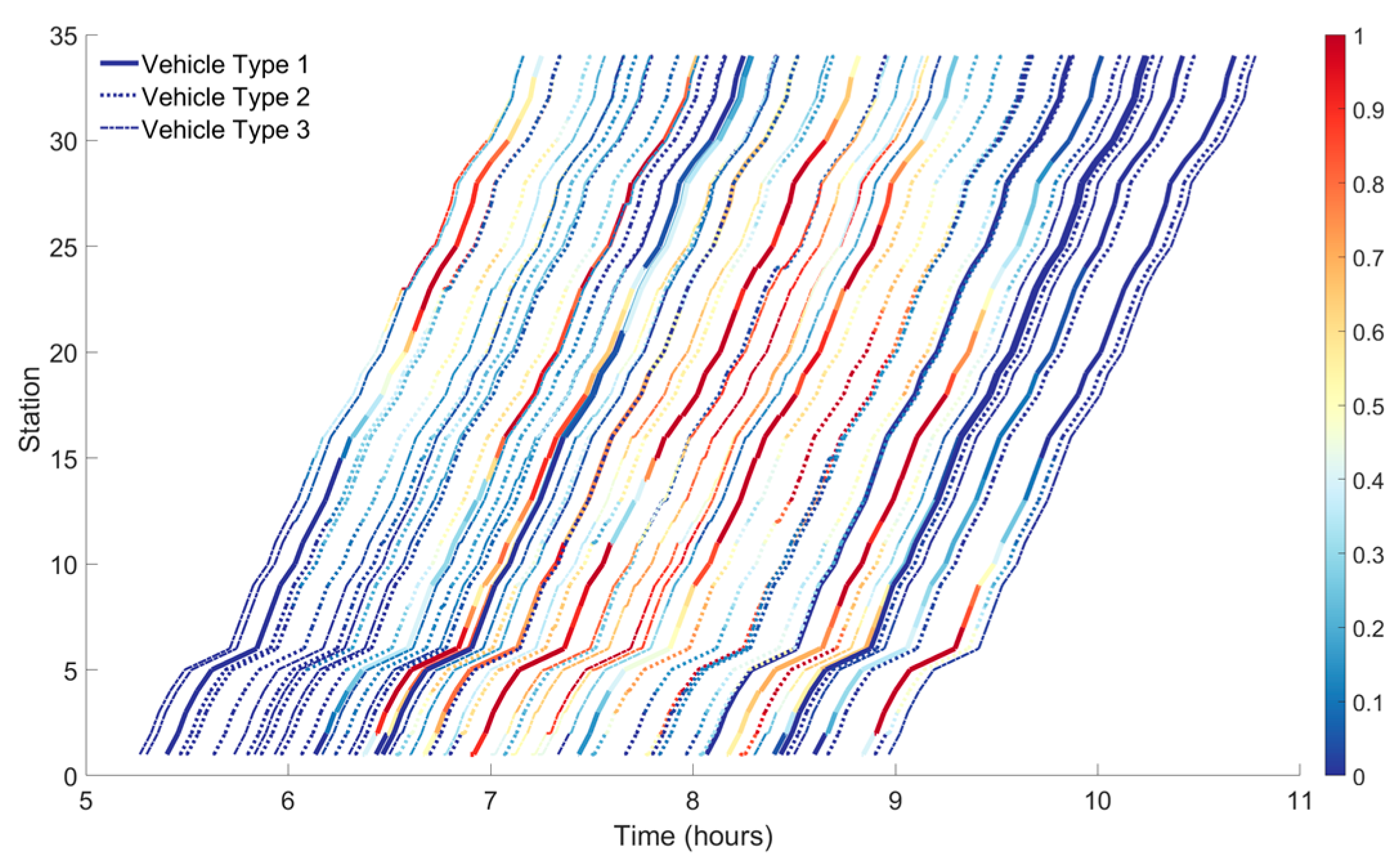
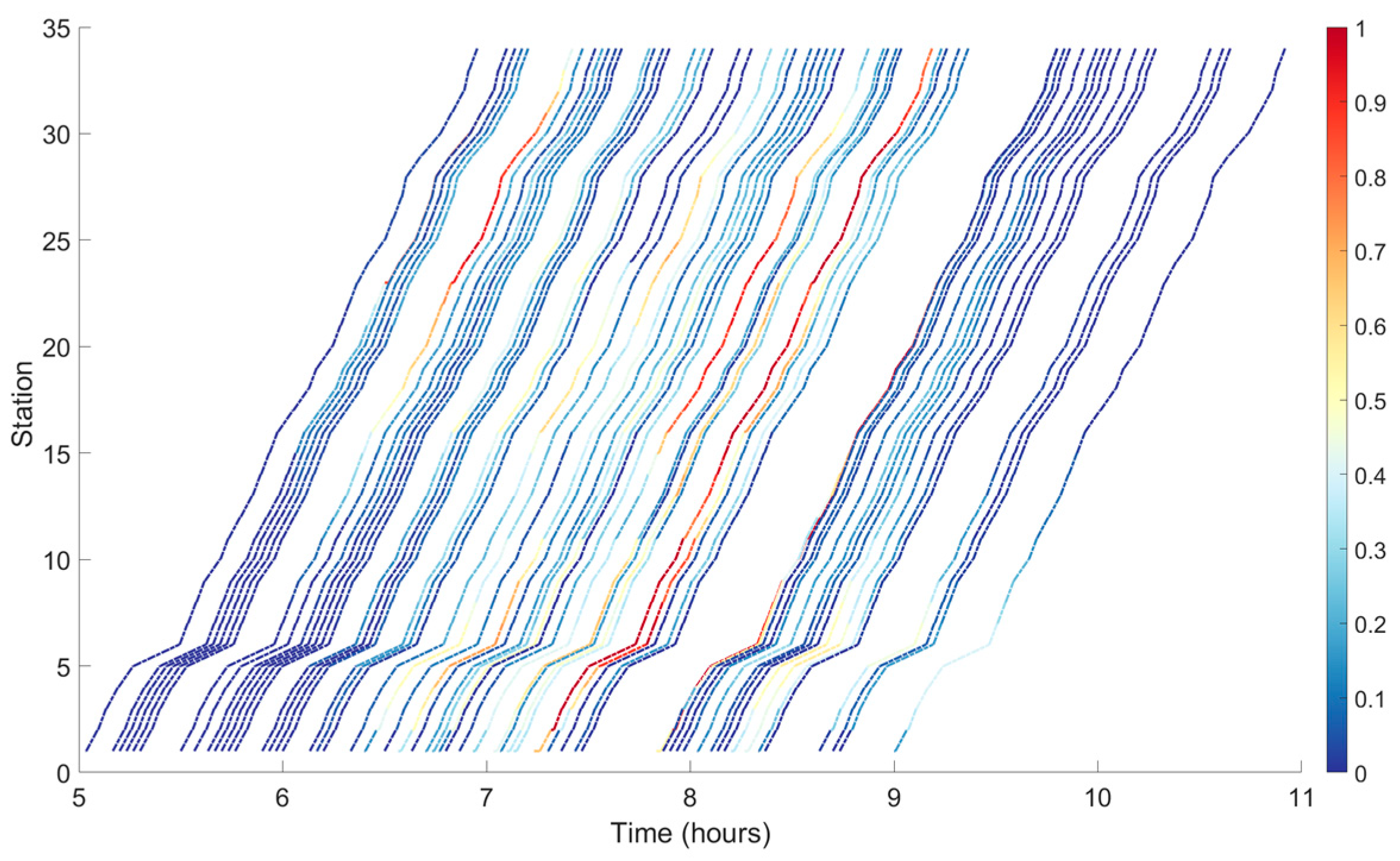
5.3.2. Scheduling Decisions

Figure 15 and Figure 16 show the spatiotemporal diagrams of the operating scenarios for the modular and fixed-capacity buses in the appointment-based travel mode. The horizontal axis represents the time points, while the vertical axis represents the bus stations. All bus trips in progress are shown in the graphs. The colors in different sections of the curves indicate the bus occupancy rate (i.e., the number of passengers on board divided by the bus capacity).

The characteristic of a fixed-capacity bus system is that its operating costs are higher and less flexible. This is mainly because fixed-capacity buses have to maintain a fixed vehicle capacity during peak hours, regardless of the actual passenger load. This leads to situations of overloading or underloading during operating hours, wasting bus capacity and resources. In contrast, the appointment-based modular bus scheduling system is more flexible in operation, allowing dynamic adjustments based on actual demand. A visual comparison shows that the appointment-based modular bus system effectively utilizes bus capacity. The color changes in the curve are smoother, indicating that the system can rationally arrange bus operations based on demand, avoiding unnecessary empty or overloaded situations. It can better adapt to actual passenger flow demands, improving the overall efficiency of the public transport system.

Figure 17 illustrates the skip-stop strategy of the appointment-based bus at each station. The blue color indicates that the vehicle stops at the station, providing boarding and alighting services to passengers, reflecting the normal operation of the system at high-demand stations. In contrast, the red color indicates that the vehicle chooses to skip the station, which can be due to a number of reasons. Firstly, it could be because the skipped station has low demand, meaning that relatively few passengers board at this station. Therefore, the vehicle chooses not to stop here to improve overall operational efficiency. Secondly, this behavior may be related to the destination of passengers on board, meaning that most passengers at this station do not have it as their final destination. Hence, the vehicle chooses to skip it to avoid unnecessary stops.

The skip-stop strategy proposed in our study essentially strikes a balance between service efficiency and passenger experience. Skipping stops at low-demand stations not only saves travel time for buses but also alleviates potential delays caused by traffic congestion. This provides a flexible and viable solution to enhance the overall operational efficiency of the public transit system. Simultaneously, avoiding stops at low-demand stations reduces unnecessary waiting time for passengers, thereby improving the overall travel experience.

6. Conclusions

A novel bus scheduling model is proposed in the context of appointment-based travel, integrating traditional flexible bus operations and travel reservation systems. By dynamically grouping modular intelligent connected buses, the model achieves precise matching of passenger and vehicle scheduling based on existing fixed bus stops. Based on passenger reservation demand data, the model considers three objectives: bus operating cost, passenger travel time cost, and waiting time cost. Taking into account the impact of bus capacity constraints, the analysis includes the passenger boarding and alighting processes within the time range of station service and the dwell time for waiting. We determined the remaining number of passengers and waiting time in two overload scenarios.

The comparative study of different scheduling scenarios evaluated the service and cost of this bus scheduling system. The main conclusions of this work are summarized as follows:

(1)

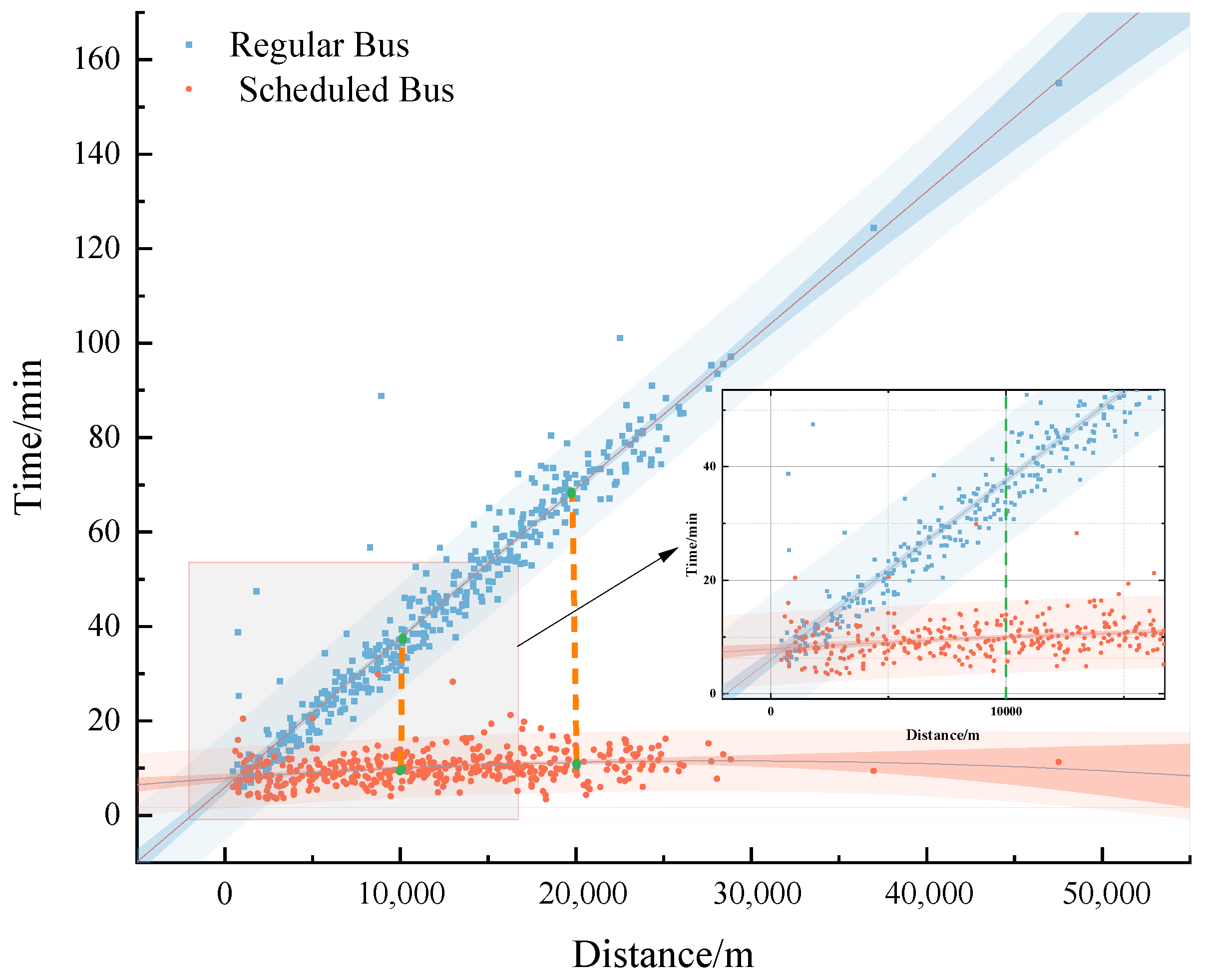
By calculating multi-scale passenger waiting times based on non-homogeneous Poisson distribution using conventional bus data, this paper effectively obtained the passenger arrival intensity at each bus station. Combined with bus departure times, the average passenger waiting time expectation at each time and spatial scale was obtained. This provides a data foundation for comparing and analyzing passenger waiting times and travel times between conventional buses and reservation-based buses.

(2)

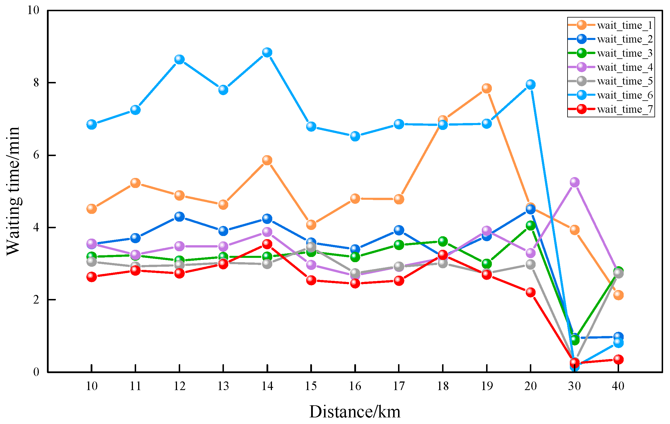
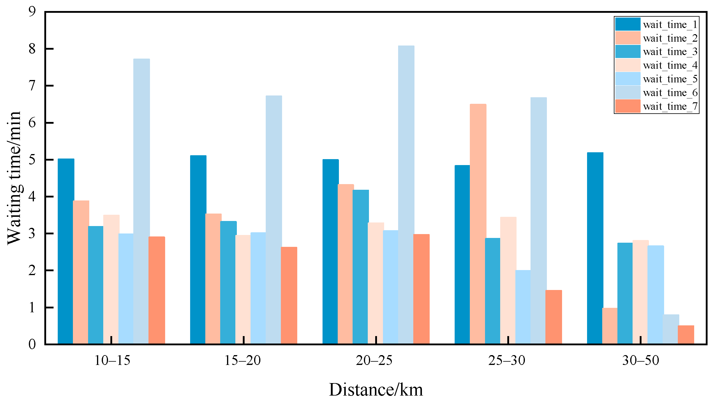
The reservation-based public transport scheduling system proposed optimizes bus schedules, resulting in significantly lower passenger waiting times compared to conventional bus services. Furthermore, the system ensures that passenger waiting times remain consistently below 4 min. Additionally, the system demonstrates notable improvements in passenger travel times. Compared to conventional fixed-capacity buses, the introduction of intelligent connected vehicle technology with dynamic grouping reduces bus operating costs by 29.7%, while simultaneously decreasing passenger waiting time by 44.15%. This enhanced flexibility in bus operations allows for dynamic adjustments based on actual demand, avoiding unnecessary empty or overloaded situations and thereby improving the overall efficiency of the public transport system.

(3)

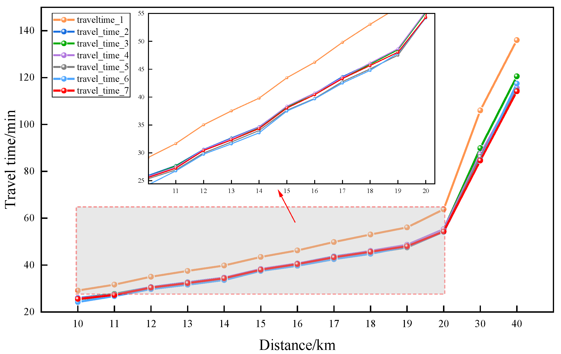
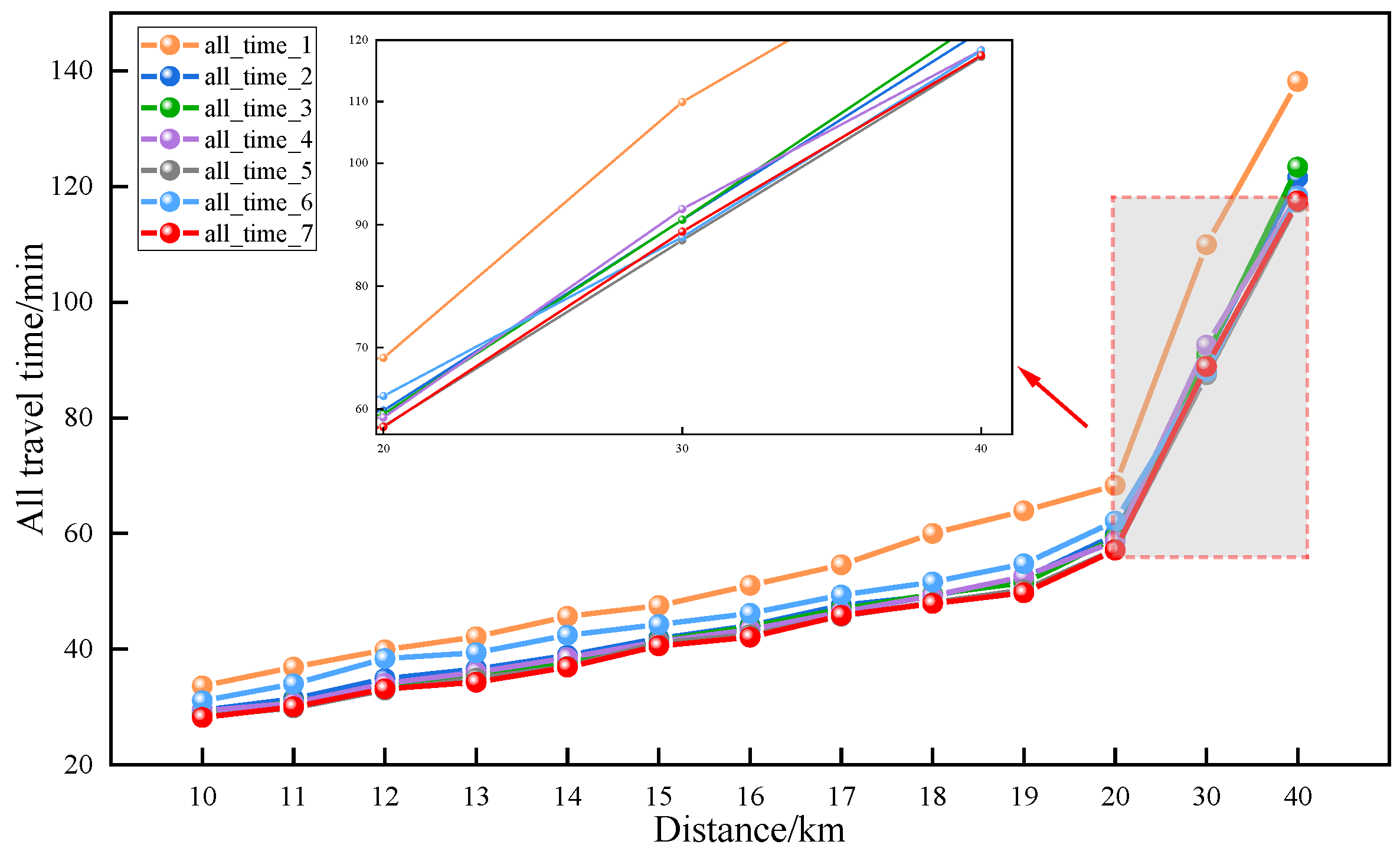
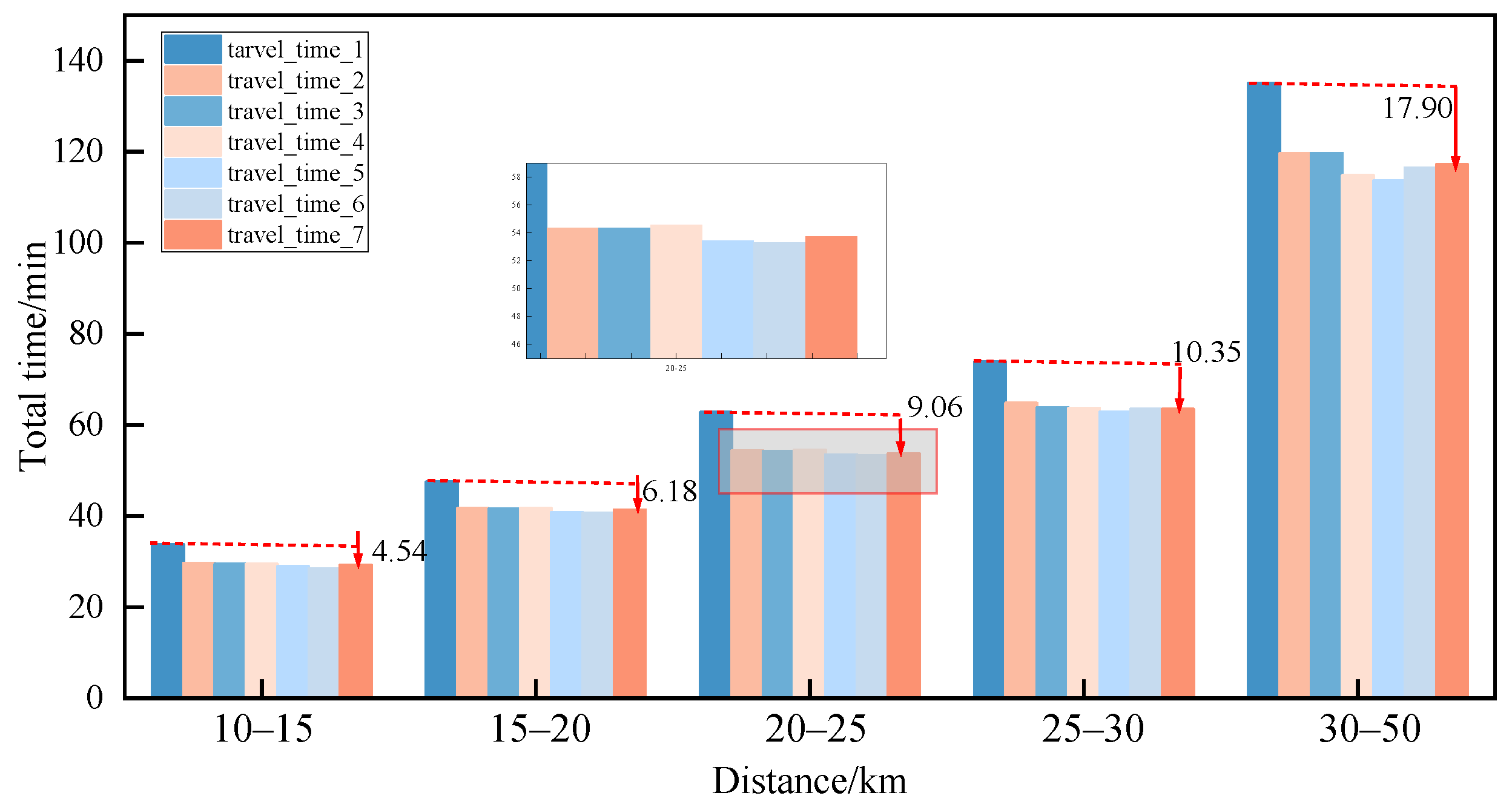
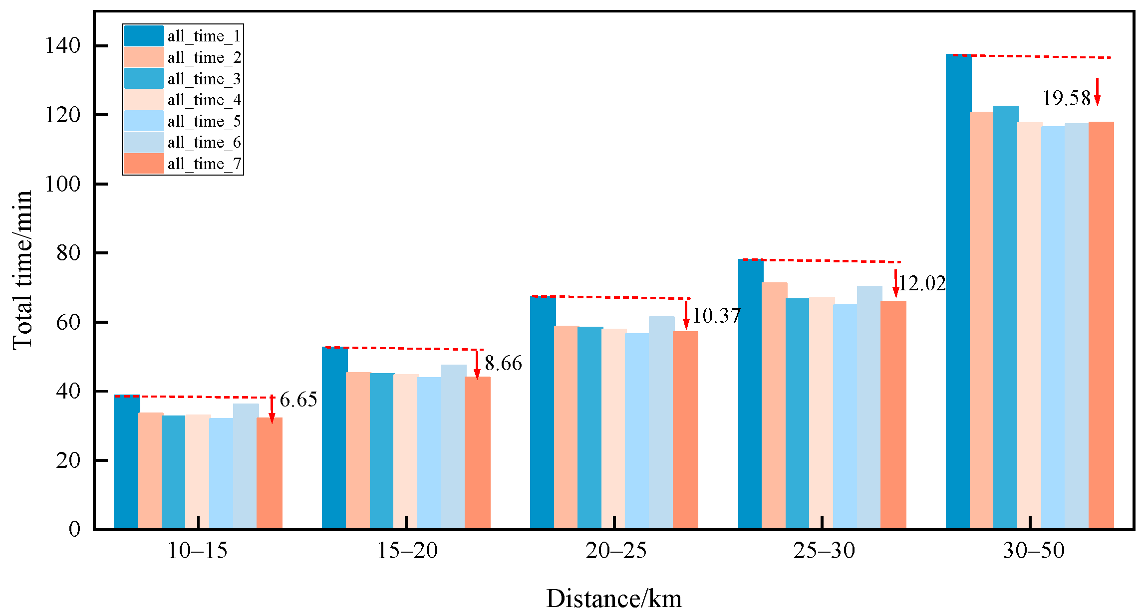
The introduced bus operation control strategy, combining skip-stop and dwell-time control in the model, significantly enhances the passenger travel experience. Specifically, the skip-stop strategy reduces passenger waiting time by 9.5%, and passenger travel time is shortened by 2.03%. With the inclusion of the dwell-time control strategy, passenger waiting time is reduced by 1.5%. When implementing both the skip-stop and dwell-time control strategies simultaneously, passenger waiting time is reduced by 15.99%, and there is also a certain improvement in passenger travel time. It is particularly noteworthy that, although the advantages of the skip-stop and dwell-time strategies are not pronounced in short-distance travel, these advantages gradually manifest with increased travel distance. This indicates that, through the judicious application of skip-stop and dwell-time control strategies, the bus system can respond more flexibly to real-time demands, avoiding unnecessary stops and waiting, successfully reducing passenger waiting time, and optimizing the overall travel experience.

Future research can focus on the following aspects: Firstly, coordination scheduling among multiple routes of reservation buses can be considered, while also taking into account the transfer behaviors of passengers. Secondly, as the volume of reservation passenger data increases, the computational efficiency of the current algorithm tends to decrease. Therefore, exploring alternative efficient solution algorithms to expedite efficiency, such as considering agent-based model optimization algorithms, could be beneficial. Finally, there is room for improvement in optimizing existing scheduling models by considering the uncertainty in actual traffic operating conditions and real-time passenger demand.

References

1. Bi, H.; Zhang, S.; Lu, F. Analysis of Decoupling Effects and Influence Factors in Transportation: Evidence from Guangdong Province, China. ISPRS Int. J. Geo-Inf. 2024, 13, 404. [Google Scholar] [CrossRef]
2. Daganzo, C.F. Checkpoint dial-a-ride systems. Transp. Res. Part B Methodol. 1984, 18, 315–327. [Google Scholar] [CrossRef]
3. Chen, Z.; Li, X.; Zhou, X. Operational design for shuttle systems with modular vehicles under oversaturated traffic: Discrete modeling method. Transp. Res. Part B Methodol. 2019, 122, 1–19. [Google Scholar] [CrossRef]
4. Wang, T.; Guo, J.; Zhang, W.; Wang, K.; Qu, X. On the planning of zone-based electric on-demand minibus. Transp. Res. Part. E Logist. Transp. Rev. 2024, 186, 103566. [Google Scholar] [CrossRef]
5. Lee, E.; Lo, H.K.; Li, M. Optimal zonal design for flexible bus service under spatial and temporal demand uncertainty. IEEE Trans. Intell. Transp. Syst. 2024, 25, 251–262. [Google Scholar] [CrossRef]
6. He, P.; Jin, J.G.; Schulte, F. The flexible airport bus and last-mile ride-sharing problem: Math-heuristic and metaheuristic approaches. Transp. Res. Part E Logist. Transp. Rev. 2024, 184, 103489. [Google Scholar] [CrossRef]
7. Liang, J.; Ren, M.; Huang, K.; Gao, Z. Data-driven timetable design and passenger flow control optimization in metro lines. Transp. Res. Part C Emerg. Technol. 2024, 166, 104761. [Google Scholar] [CrossRef]
8. Su, Y.; Yang, H. Enhancing feeder bus service coverage with multi-agent reinforcement learning: A case study in hong kong. Transp. Res. Part E Logist. Transp. Rev. 2025, 196, 103997. [Google Scholar] [CrossRef]
9. Ma, X.; Shen, X.; Zhang, Z.; Luan, S.; Chen, X. Optimization of autonomous bus scheduling based on lagrangian relaxation. China J. Highw. Transp. 2019, 32, 10–24. [Google Scholar] [CrossRef]
10. Yu, Q.; Zhang, H.; Li, W.; Song, X.; Shibasaki, R. Mobile phone GPS data in urban customized bus: Dynamic line design and emission reduction potentials analysis. J. Clean. Prod. 2020, 272, 122471. [Google Scholar] [CrossRef]
11. Papanikolaou, A.; Basbas, S. Analytical models for comparing demand responsive transport with bus services in low demand interurban areas. Transp. Lett. 2021, 13, 255–262. [Google Scholar] [CrossRef]
12. Lee, E.; Cen, X.; Lo, H.K. Scheduling zonal-based flexible bus service under dynamic stochastic demand and time-dependent travel time. Transp. Res. Part E Logist. Transp. Rev. 2022, 168, 102931. [Google Scholar] [CrossRef]
13. Ma, W.; Zeng, L.; An, K. Dynamic vehicle routing problem for flexible buses considering stochastic requests. Transp. Res. Part C Emerg. Technol. 2023, 148, 104030. [Google Scholar] [CrossRef]
14. Liu, X.; Qu, X.; Ma, X. Improving flex-route transit services with modular autonomous vehicles. Transp. Res. Part E Logist. Transp. Rev. 2021, 149, 102331. [Google Scholar] [CrossRef]
15. Guo, R.; Guan, W.; Vallati, M.; Zhang, W. Modular Autonomous Electric Vehicle Scheduling for Customized On-Demand Bus Services. IEEE Trans. Intell. Transp. Syst. 2023, 24, 1–12. [Google Scholar] [CrossRef]
16. Tian, Q.; Lin, Y.H.; Wang, D.Z.W. Joint scheduling and formation design for modular-vehicle transit service with time-dependent demand. Transp. Res. Part C Emerg. Technol. 2023, 147, 103986. [Google Scholar] [CrossRef]
17. Dai, Z.; Liu, X.C.; Li, H.; Wang, M.; Ma, X. Semi-autonomous bus platooning service optimization with surrogate modeling. Comput. Ind. Eng. 2023, 175, 108838. [Google Scholar] [CrossRef]
18. Wu, M.; Yu, C.; Ma, W.; An, K.; Zhong, Z. Joint optimization of timetabling, vehicle scheduling, and ride-matching in a flexible multi-type shuttle bus system. Transp. Res. Part C Emerg. Technol. 2022, 139, 103657. [Google Scholar] [CrossRef]
19. Dai, Z.; Liu, X.C.; Chen, Z.; Guo, R.; Ma, X. A predictive headway-based bus-holding strategy with dynamic control point selection: A cooperative game theory approach. Transp. Res. Part B Methodol. 2019, 125, 29–51. [Google Scholar] [CrossRef]
20. Vismara, L.; Chew, L.Y.; Saw, V. Optimal assignment of buses to bus stops in a loop by reinforcement learning. Phys. A 2021, 583, 126268. [Google Scholar] [CrossRef]
21. Tang, C.; Shi, H.; Liu, T. Optimization of single-line electric bus scheduling with skip-stop operation. Transp. Res. Part D-Transp. Environ. 2023, 117, 103652. [Google Scholar] [CrossRef]
22. Wu, W.; Zhu, Y.; Liu, R. Dynamic scheduling of flexible bus services with hybrid requests and fairness: Heuristics-guided multi-agent reinforcement learning with imitation learning. Transp. Res. Part B Methodol. 2024, 190, 103069. [Google Scholar] [CrossRef]
23. Ma, H.; Yang, M.J.; Li, X. Integrated optimization of customized bus routes and timetables with consideration of holding control. Comput. Ind. Eng. 2022, 175, 108886. [Google Scholar] [CrossRef]
24. Rodriguez, J.; Koutsopoulos, H.N.; Wang, S.; Zhao, J. Cooperative bus holding and stop-skipping: A deep reinforcement learning framework. Transp. Res. Part C Emerg. Technol. 2023, 155, 104308. [Google Scholar] [CrossRef]
25. Bajada, J.; Grech, J.; Bajada, T. Deep reinforcement learning of autonomous control actions to improve bus-service regularity. In Proceedings of the Artificial Intelligence. ECAI 2023 International Workshops, Kraków, Poland, 30 September–4 October 2023; Springer Nature: Cham, Switzerland, 2024. [Google Scholar] [CrossRef]
26. Liu, Z.; Yu, P.; Li, J. Distribution network planning of distributed power sources and generalized energy storage considering operational characteristics. Electr. Power Autom. Equip. 2023, 43, 72–79. [Google Scholar] [CrossRef]
27. Xiao-Chun, Z.; Yong, G.; Zhuang, Y.U.; Yu-Huan, W.; Jian, A.N. Passenger average waiting time estimation based on bus GPS and IC card data. J. Transp. Syst. Eng. Inf. Technol. 2019, 19, 236–241. Available online: http://www.tseit.org.cn/EN/abstract/abstract19930.shtml (accessed on 10 March 2025).
28. Lu, H.; Burge, P.; Heywood, C.; Sheldon, R.; Lee, P.; Barber, K.; Phillips, A. The impact of real-time information on passengers’ value of bus waiting time. Transp. Res. Procedia 2018, 31, 18–34. [Google Scholar] [CrossRef]
29. Gong, H.; Chen, X.; Yu, L.; Wu, L. An application-oriented model of passenger waiting time based on bus departure time intervals. Transp. Plan. Technol. 2016, 39, 424–437. [Google Scholar] [CrossRef]
Figure 1. Travel scenarios in public transit modes.
Sustainability 17 02645 g001
Figure 2. Time–space diagram of a bus trip as an example.
Sustainability 17 02645 g002
Figure 3. Relationship between upper and lower levels in the dual-layer optimization model.
Sustainability 17 02645 g003
Figure 4. The solution process of the double-layer nested particle swarm optimization model.
Sustainability 17 02645 g004
Figure 5. Schematic diagram of Bus Route 300’s inner loop in Beijing.
Sustainability 17 02645 g005
Figure 6. Passenger arrival curves at selected stations.
Sustainability 17 02645 g006
Figure 7. Comparison chart of total travel time for conventional buses and reservation-based buses.
Sustainability 17 02645 g007
Figure 8. Waiting times for passengers in different scenarios.
Sustainability 17 02645 g008
Figure 9. Travel times for passengers in different scenarios.
Sustainability 17 02645 g009
Figure 10. Total travel time for passengers.
Sustainability 17 02645 g010
Figure 11. Total travel time of passengers under different distance intervals.
Sustainability 17 02645 g011
Figure 12. Waiting time for different travel distances.
Sustainability 17 02645 g012
Figure 13. Operating costs and passenger waiting time costs in different scenarios.
Sustainability 17 02645 g013
Figure 14. Costs of different scenario scheduling strategies.
Sustainability 17 02645 g014
Figure 15. Schematic diagram of the operational schedule for modular buses under the appointment-based travel mode.
Sustainability 17 02645 g015
Figure 16. Schematic diagram of the operational schedule for fixed-capacity buses under the appointment-based travel mode.
Sustainability 17 02645 g016
Figure 17. Reservation bus stop strategy diagram.
Sustainability 17 02645 g017