Abstract
Ultra-short-term wind speed forecasting is crucial for ensuring the safe grid integration of wind energy and promoting the efficient utilization and sustainable development of renewable energy sources. However, due to the arbitrary, intermittent, and volatile nature of wind speed, achieving satisfactory forecasts is challenging. This paper proposes a combined forecasting model using a modified pelican optimization algorithm, variational mode decomposition, and long short-term memory. To address issues in the current combination model, such as poor optimization and convergence performance, the pelican optimization algorithm is improved by incorporating tent map-based population initialization, Lévy flight strategy, and classification optimization concepts. Additionally, to obtain the optimal parameter combination, the modified pelican optimization algorithm is used to optimize the parameters of variational mode decomposition and long short-term memory, further enhancing the model’s predictive accuracy and stability. Wind speed data from a wind farm in China are used for prediction, and the proposed combined model is evaluated using six indicators. Compared to the best model among all compared models, the proposed model shows a 10.05% decrease in MAE, 4.62% decrease in RMSE, 17.43% decrease in MAPE, and a 0.22% increase in R2. The results demonstrate that the proposed model has better accuracy and stability, making it effective for wind speed prediction in wind farms.
1. Introduction
Due to the worldwide consensus to attain carbon neutrality, expanding renewable energy sources has increasingly become the norm. Renewable energy like solar, wind, and hydro power produce much lower carbon emissions than traditional fossil fuel-based energy. Among renewable options, wind power stands out as having especially prominent low-carbon attributes since it generates fewer emissions than alternatives. Additionally, wind resources are widely available in large quantities, yielding significant reserves of wind power that can be tapped for energy production [1]. Therefore, wind power has been increasingly valued by countries worldwide. In recent years, the new installed capacity of global wind power has shown a rapid upward trend, rising from 50.7 GW in 2018 to 93 GW in 2021. And as of 2021, the cumulative installed global wind power capacity had arrived at 837 GW. Moreover, according to the forecast of the Global Wind Energy Council, over the next five years (2022–2026), there will be an increase of 557 GW in installed wind power capacity globally, with a compound annual growth rate of 6.6%. By 2026, the new installed capacity of wind power globally will reach 128.8 GW [2]. However, wind energy exhibits intermittency and stochastic fluctuations, where changes in WS (wind speed) directly affect the active power and reactive power of wind farms, resulting in unstable power output. With the rapid development of wind power generation, the issues caused by the unstable output power of wind farms, such as difficulties in power system dispatching and operation, as well as significant wind curtailment, have become increasingly prominent. These directly impact the safe, stable, and economically efficient operation of the power grid [3,4]. The impact of WS prediction on wind power generation is significant, as accurate forecasting allows for the better planning and management of wind farms. By predicting WS with precision, operators can optimize the operation of turbines, adjust the power output accordingly, and anticipate fluctuations in energy production. This leads to the improved efficiency, reduced costs, and increased reliability of wind power generation systems. Additionally, accurate WS prediction enables grid operators to integrate wind energy more effectively into the overall energy mix, contributing to a more sustainable and reliable power supply. Therefore, accurate WS prediction can effectively and economically solve problems caused by the instability of wind power and wind power integration problems.
WS forecasting can be classified from different angles. According to the forecasted time horizon, WS forecasts can be categorized into ultra-short-term, short-term, medium-term, and long-term forecasts [5]. And the ultra-short term is a few seconds to 30 min, the short term is 30 min to 6 h, the medium term is 6 h to a day, and the long term is a day to a few weeks. In addition, WS forecasts can also be categorized into physical models, statistical models, and artificial intelligence models according to different prediction models [6]. The physical model is based on computational fluid dynamics and is built using detailed information such as meteorological information, the topographic features of the location of the wind farm, and surface roughness. Therefore, the NWP (numerical weather prediction) model is a typical physical model. Feng et al. [7] proposed a physics-based prediction method using WS as input data for numerical weather forecasting. Moreover, Liu et al. [8] greatly enhanced the precision of wind power prediction by improving the accuracy of NWP. And Li et al. [9] proposed a correction strategy for NWP to further enhance the precision of wind power prediction. The biggest advantage of a physical model is that it does not require historical operation data from wind farms, and it is suitable for newly built farms or those with incomplete data. However, physical models rely on rich and accurate meteorological, terrain, and other environmental data, and need to simulate the changes in meteorological factors such as WS and direction under the local effects of wind farms. The modeling complexity of physical models is high, and there are many uncertain links. Due to the limitations of model accuracy and simulation ability, systematic deviations may occur. Because of the high computational cost of numerical weather forecasting, the physical model based on numerical weather forecasting is not suitable for short-term WS forecasting, so it is mostly used for medium- and long-term WS forecasting [10]. Statistical models are established by studying the mapping relationship between input data and output data in historical data, and their main processes include model identification, parameter estimation, and model validation. Traditional statistical models include the Kalman filter model [11], AR (autoregressive) model [12], MA (moving average) model [13], ARMA (autoregressive moving average) model [14], and ARIMA (autoregressive integrated moving average) model [15]. Compared to physical models, statistical models have simple methods and use a single type of data, but their ability to process sudden changes is poor. At the same time, this model type requires a large amount of historical operating data, so it is not suitable for newly built or incomplete wind farms. In addition, the performance of statistical models deteriorates as the prediction time increases, and it is difficult to obtain excellent forecasting results for nonlinear and unstable WS data [16]. Moreover, the artificial intelligence model is derived from statistical methods and is built through the repeated learning and training of data relationships based on large amounts of historical data. And common artificial intelligence models include the SVM (support vector machine) [17], BP (backpropagation) neural network [18], deep learning model [19,20,21], DBN (deep belief network) [22], reinforcement learning model [23], and broad learning models [24]. Nevertheless, a single artificial intelligence model has the disadvantages of being easily trapped in local minima, overfitting, underfitting, etc., and cannot fully capture all information about WS sequences. In order to overcome these shortcomings and make full use of the advantages of a single model and various methods, building a combined model to predict WS has gradually become a popular topic of research [25].
At present, the most common combined forecasting methods are the combination of different models and the combination of models and algorithms. In terms of different model combinations, Neto et al. [26] constructed a hybrid model that combines linear statistical and artificial intelligence (AI) forecasters, which can effectively overcome the shortcomings of single models. Moreover, Cheng et al. [16] combined the four models of BP, a random vector functional link network, ENN (evolutionary neural network), and GRNN (generalized regression neural network) to form a new hybrid model, which can better utilize the characteristics of each model and make up for the inadequacy of a single model. Moreover, Shahzad et al. [27] proposed a new combined model based on ARAR (autoregressive–autoregressive) and ANN (artificial neural network) models, which was experimentally demonstrated to better predict WS time series datasets. And Liang et al. [28] combined the RNN (recurrent neural network) and CNN (convolutional neural network) to propose a new method. On the other hand, there are also many relevant studies on the combination of models and algorithms. According to the different functions of algorithms, they can be divided into two categories: optimization algorithms and decomposition methods. Because of their strong versatility, high efficiency, and simple implementation, swarm intelligence optimization algorithms have become a popular topic of research in the field of artificial intelligence and intelligent computing [29,30] and have been widely used in the parameter optimization of WS prediction models. For instance, there are some common optimization algorithms that have been combined with models, which include PSO (particle swarm optimization) [31], the WOA (whale optimization algorithm) [32], the DA (dragonfly algorithm) [33], GWO (grey wolf optimization) [34], etc. WS data have the characteristics of strong nonlinearity and non-stationarity. Signal decomposition methods have been gradually introduced into WS prediction in recent years because of their outstanding role in denoising and extracting signal features in complex signal processing. They are mainly used in combination with various models for data preprocessing. In WS prediction, common decomposition methods include EMD (empirical mode decomposition) [35], VMD (variational mode decomposition) [36], EEMD (ensemble empirical mode decomposition) [37], CEEMD (complementary ensemble empirical mode decomposition) [38], etc. Ibrahim et al. [39] proposed a combined prediction model based on AD-PSO, Guided WOA, and LSTM (long short-term memory); the experiment showed that the LSTM optimized by AD-PSO and Guided WOA has strong predictive performance. Altan et al. [40] proposed a combined prediction model based on a single model, namely, LSTM, a decomposition method, namely, ICEEMDAN (improved complementary ensemble empirical mode decomposition with adaptive noise), and an advanced optimization algorithm, namely, GWO; the combined model could better capture the nonlinear characteristics of WS data and had good prediction accuracy.
While combination models integrate multiple individual models and techniques to leverage their respective strengths and compensate for limitations, existing combination models still have some issues. First, determining optimal model integration and weighting is challenging when combining multiple model types. Simply combining various models often does not significantly improve combination model performance. Currently, there is a lack of comparative analysis on the roles of various types of techniques in composite model research. The theoretical construction of composite models needs further improvement. Second, when combining models with optimization algorithms, most existing combination models directly introduce the algorithm without improvements, limiting the algorithm’s functionality. Third, when combining models with decomposition methods, decomposition parameter settings significantly impact results. Existing models often use experiential parameter settings rather than effectively optimizing parameter combinations. Finally, combination models’ complex structures and numerous parameters generally cause long prediction times. These issues directly affect model prediction performance.
Based on the above analysis, the primary factors that impact the performance of a WS prediction model are as follows: First, WS data preprocessing is inadequate. WS data sources contain much noise and interference, making complete and precise data collection challenging. Existing preprocessing cannot effectively reduce noise and extract time series information. Second, model parameter optimization is insufficient. The many parameters in combination models often make conventional intelligent optimization algorithms inaccurate and slow in application, negatively affecting model prediction. Optimization algorithm convergence, search efficiency, and parameter settings need further development and improvement. Finally, combination model construction is unreasonable. WS characteristics like strong randomness, intermittency, and volatility require models with robust adaptive abilities. Existing models lack integrated advanced data mining and parameter optimization technologies for performance optimization. Therefore, it is evident that existing models have certain limitations and fail to meet the increasing demand for WS prediction performance, especially in terms of selecting and optimizing individual techniques within combination models, leaving significant room for improvement. To address these issues, this paper proposes a hybrid ultra-short-term WS forecasting model based on a modified pelican optimization algorithm. Firstly, targeting the common problems of swarm intelligence optimization algorithms, such as being easily trapped in local optima and insufficient optimization precision, an MPOA (modified pelican optimization algorithm) is introduced. This algorithm enhances the diversity of the initial population by incorporating chaotic mapping, improves the algorithm’s local exploration capability by introducing Lévy flight strategy, and dynamically adjusts critical parameters to enhance adaptability, thereby achieving overall performance enhancement in algorithm optimization. Secondly, to address the challenges of parameter abundance and the difficulty in combination optimization in VMD, a combined VMD key parameter optimization method using the MPOA and sample entropy is proposed, enabling the deep exploration of WS’s nonlinear variation characteristics. Finally, to tackle the problem of numerous hyperparameters in LSTM and the difficulty in achieving parameter optimization manually, the MPOA is applied to optimize the hyperparameters of LSTM, resulting in a significant improvement in LSTM’s predictive performance. Additionally, this paper conducts comparative simulation experiments between the proposed combination model and other models using WS data from a wind farm in eastern China, validating the predictive performance of the model.
The primary contributions of this paper include the following:
- A modified pelican optimization algorithm is proposed. First, the tent map is applied for population initialization and the Lévy flight factor is introduced. Second, algorithm applications to different dimensional problems are classified and optimized. Finally, improved algorithm optimization performance is verified through test functions. The proposed modified pelican optimization algorithm not only effectively enhances the algorithm’s global and local search capabilities but also provides a new avenue for optimizing swarm intelligence algorithms;
- The original WS data are modally decomposed by VMD. Through the use of sample entropy as an evaluation metric to determine K (the modal decomposition number) for VMD, and of RMSE (root mean square error) as the objective function for the MPOA, the alpha (moderate bandwidth constraint) and tau (noise tolerance) of the other two parameters of VMD are optimized. Applying VMD with the optimized parameter combination for WS data decomposition significantly reduces the nonlinearity and instability characteristics of the original WS data, effectively exploring the features of WS data. By introducing the composite evaluation metrics of sample entropy and RMSE in the parameter optimization of the WS signal decomposition strategy VMD, the data preprocessing technique effectively removes noise while retaining the main features of the original signal sequence, significantly improving the effectiveness of WS prediction;
- The MPOA is applied to optimize LSTM model hyperparameters including the iteration number, first LSTM layer neuron number, second LSTM layer neuron number, and learning rate. Through hyperparameter optimization, the MPOA significantly strengthens LSTM predictive capabilities;
- A combined ultra-short-term WS forecasting model based on the modified pelican optimization algorithm is proposed, combining the MPOA, VMD, and LSTM. The WS prediction process based on the combined model is constructed. The proposed VMD-MPOA-LSTM model provides a new effective method to improve ultra-short-term WS prediction model performance;
- A comprehensive and effective evaluation of the developed combined model’s performance is carried out. The evaluation system uses three experiments and six performance indicators to effectively assess prediction accuracy and stability. Experimental analysis specifically determines optimization algorithm and data decomposition method impacts on the prediction model, providing a theoretical and practical basis for combined model construction.
The rest of this paper is organized as follows: In Section 2, the methodology is introduced, including optimization algorithms, data preprocessing techniques, and LSTMs and their combined models. And in Section 3, the experimental procedures of the proposed combined model are illustrated, and the comparative experimental results of different models are shown. Additionally, the precision and validity of the proposed model are discussed and validated in Section 4. Concluding remarks are then provided in Section 5.
2. Methodology
This section details the methodologies used to build the hybrid forecasting model, including the modified pelican optimization algorithm, variational mode decomposition, LSTM neural network, and framework of the proposed combined model. The modified pelican optimization algorithm is applied to optimize the parameters of VMD and LSTM, enhancing the capabilities of the hybrid forecasting model.
2.1. Modified Pelican Optimization Algorithm
2.1.1. Pelican Optimization Algorithm
The pelican optimization algorithm is a novel swarm intelligence algorithm proposed by Trojovský et al. [41], which simulates the natural behavior of pelicans during hunting. The procedural steps for optimization using the algorithm are detailed below.
- (1)
- Initialization
Initially, the population is randomly generated in a certain range according to Equation (1).
where represents the value of the jth variable for the ith pelican in the population. The population size is N, and the dimension is m. rand denotes a randomly generated number between 0 and 1. and represent the lower and upper bounds, respectively.
In the proposed POA, the population members consisting of pelicans are represented by a population matrix, defined in Equation (2).
where is the population matrix of pelicans and is the ith pelican member of the population.
In the POA, every constituent of the population represents a potential solution in the form of a pelican. Thus, the objective function for the given problem can be evaluated for each candidate solution. The resulting objective function values for all candidates are contained in a vector called the objective function vector, defined in Equation (3).
where denotes the objective function vector comprising the objective function values computed for each prospective solution. refers to the objective function value of the ith potential solution.
- (2)
- Location Update
The location update process in the POA simulates the foraging behavior of pelicans, which is divided into two phases: exploration and exploitation.
In the exploration phase, pelicans first locate potential prey and then move toward areas where prey is detected. The prey location is arbitrarily created inside the search field, allowing the POA to better probe the problem domain. This increases the algorithm’s ability to thoroughly traverse the problem resolution landscape. The pelican’s movement strategy toward the prey position is mathematically modeled as follows:
where is the position of the prey in the jth dimension, and represents the objective function value of the prey. is a random number taking either 1 or 2 as its value. When , it allows each individual pelican to increase its movement distance and enter new areas of the search space for further exploration.
After the exploration phase, the objective function value at the pelican’s new position is compared to the objective function value at the prey location. The position with the lower objective function value is selected, whether it be the prey location or the pelican’s new explored position. This comparison helps guide the pelicans toward better solutions within the search space. The update method is as follows:
where is the new position of the ith pelican after phase 1 exploration and is its corresponding objective function value.
In the exploitation phase, pelicans utilize a different foraging strategy. After reaching the target area located in phase 1, pelicans beat their wings over the water to steer prey together and capture it in their throat pouches. Mathematically modeling this behavior increases the POA’s local search abilities and resource utilization within identified promising regions. More prey can be captured within the attack area using this exploitation strategy. The pelican hunting process is formally simulated using the following mathematical model:
where represents the new position of the pelican i in dimension j after exploitation in phase 2. is a constant at 0.2, and defines the proximity searching radius of , where t refers to the ongoing iteration and T is the final iteration.
During this phase, Equation (7) models an effective acceptance–rejection process for the new pelican position determined by local exploitation.
where and represent the new position and corresponding objective value of the ith pelican after applying the phase 2 local exploitation strategy.
- (3)
- Step Repetition
Once all population members have undergone the exploration and exploitation phases to update their positions, the optimal solution found thus far is refreshed based on the new population distribution and corresponding objective function values. The algorithm then iterates, recycling through the stipulated POA steps as per Equations (4)–(7). This iterative process continues until the full execution is complete. Ultimately, the best candidate solution discovered over all the iterations is offered as a suboptimal solution to the optimization problem. By progressively improving the candidate solutions over multiple iterations in this manner, the POA aims to converge toward the most suitable solution.
2.1.2. Improvement in the Algorithm
- (1)
- Population initialization based on tent map
During population initialization, the POA adopts a similar approach to other metaheuristic optimization algorithms, employing a randomly generated method. This approach results in a lack of diversity within the population. The diversity in the population directly influences the convergence accuracy and speed of the optimization algorithm. A well-diversified population is advantageous for the algorithm to quickly identify the global optimal solution. Therefore, introducing an appropriate population initialization method that covers a broader range of the solution space is essential. A chaotic sequence has the characteristics of regularity, randomness, and ergodicity. Fusing the POA’s initial population with chaos provides better diversity compared to full randomization. Chaos mainly generates a chaotic sequence through mapping the relationship of (0, 1), and then it converts the map to the population individual space. Many types of chaos exist, with logistic mapping being most common. However, logistic mapping has poor ergodicity and sensitivity to initial parameters, with high mapping point density at the edges and lower density in the middle region. Tent mapping has better uniformity than logistic mapping [42,43]. Therefore, tent mapping was selected to initialize the population in this research. The tent map is a piecewise linear function with parameter μ defined as follows:
where is the chaos parameter, which is proportional to the chaos.
- (2)
- Classification value of I value
It can be known from Equation (4) that I is a random number, representing the displacement of individuals in the group. Thus, it represents the performance of entering a new search space. When the value of I is small, individuals can effectively explore local regions, thus benefiting the later-stage optimization of the population and making it more suitable for low-dimensional functions. When the value of I is large, the individuals’ movement space expands, allowing for a broader exploration range and escaping local optima. Consequently, this is advantageous for the early-stage optimization of the population and is more suitable for high-dimensional functions with multiple local optima. In the POA, I is a fixed value, preventing it from achieving optimal optimization performance across different types of functions. Therefore, selecting different values of I for different function types can effectively enhance the optimization performance of the POA. In this paper, I is classified and selected based on the function’s dimension as follows:
- (3)
- Introducing the Lévy flight strategy
In the basic POA, especially for high-dimensional function optimization, pelican individuals can “clump” as iterations increase, causing the algorithm to fall into local extrema. A Lévy flight involves searching the solution space through random walks. The step length of a Lévy flight follows a Lévy stable distribution, enabling it to conduct a wide-ranging search in the solution space and making the movement of individuals more agile. The Lévy flight can break this “clump” phenomenon by increasing population diversity and improving local exploration. Therefore, Lévy flights are introduced into the POA’s position update to obtain
is the Lévy random search path and satisfies
where represents a random number following a normal distribution, and represents the flight time.
Figure 1 depicts a flowchart of the improved POA. The modifications are highlighted using red text boxes.
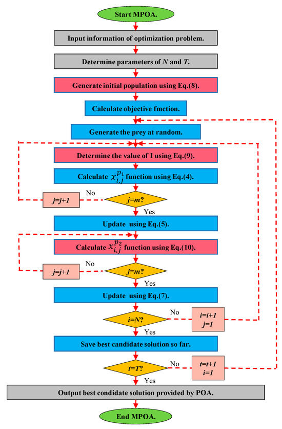
Figure 1.
Flowchart of MPOA.
2.1.3. The Test of the MPOA
The CEC (Congress on Evolutionary Computation) benchmark test functions are commonly used to test swarm intelligence algorithms, comprising 23 classical functions divided into three categories: unimodal, multimodal, and low-dimensional multimodal. Unimodal functions evaluate an algorithm’s convergence rate, precision, and local search capabilities in high-dimensional spaces. Multimodal functions, containing multiple local optima, assess an algorithm’s ability to find the global optimum through broad search space exploration. Low-dimensional multimodal functions specifically examine algorithm performance under low-dimensional conditions. Using both unimodal and multimodal benchmark functions of varying dimensions allows the comprehensive testing of an algorithm’s convergence properties, local refinement capabilities, and global exploration tendencies. Nine test functions were selected from the CEC benchmarks for this research, representing the most commonly used typical functions across the three categories, with variable dimensions ranging from 2 to 30. This provides strong test performance to comprehensively evaluate optimization algorithm capabilities. Table 1, Table 2 and Table 3 show details for each function.

Table 1.
Unimodal test functions.
Table 2.
Multimodal test functions.
Table 3.
Low-dimension multimodal test functions.
To validate the efficacy of the MPOA, this study selected 9 benchmark functions from the classic benchmark functions according to actual needs and used Matlab®(2021b) to optimize the calculation. Then, the optimization results of the MPOA and several popular swarm intelligence optimization algorithms (PSO, MFO, WOA) were compared and analyzed. The parameters selected for each algorithm are listed in Table 4. All optimization calculations in Matlab® were performed on a desktop computer with 8 GB memory, a Ryzen 8-core processor, and a main frequency of 3.4 GHz.
Table 4.
Parameter values used in MPOA, POA, PSO, MFO, and WOA.
All algorithms were limited to a specified maximum number of iterations based on their convergence speed. For functions F1–F6, the limit was 1000 iterations, and for F7–F9, it was 100 iterations. Each algorithm independently ran 30 times on each benchmark function to obtain statistically valid results. The performance metrics reported include the mean, median, standard deviation, best, and worst objective function values over the 30 runs, detailed in Table 5, Table 6 and Table 7. Convergence curves plotting optimization progress over iterations were also generated for each algorithm and function, as illustrated in Figure 2.
Table 5.
A comparison of different methods in solving the unimodal test functions in Table 1 at 30 dimensions.
Table 6.
A comparison of different methods in solving the multimodal test functions in Table 2 at 30 dimensions.
Table 7.
A comparison of different methods in solving the low-dimension multimodal test functions in Table 3.
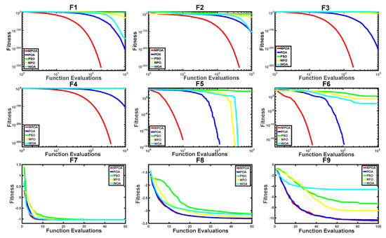
Figure 2.
Convergence characteristic curves for MPOA, POA, PSO, MFO, and WOA in solving the test function.
The results in Table 5, Table 6 and Table 7 and Figure 2 show that the MPOA demonstrated significantly better convergence accuracy and speed compared to the other four algorithms when optimizing F1–F6. For F7–F9, its convergence accuracy and speed were slightly better than the POA but still substantially improved over the other three algorithms, with superior stability.
2.2. MPOA-VMD
2.2.1. VMD
VMD is an adjustable signal processing approach developed by Dragomiretskiy et al. [44] that concurrently decomposes a multivariate signal into several univariate signals, including amplitude modulation (AM) and frequency modulation (FM) signals. This avoids issues like end effects and spurious components that can arise with iterative decomposition methods. Additionally, VMD capably handles nonlinear and non-stationary signals. Unlike traditional EMD, the IMFs in VMD are reconceptualized as AM or FM signals and expressed as
where the instantaneous amplitude is represented by and the instantaneous phase by . VMD is based on a variational problem framework, which achieves the adaptive decomposition of signals by determining the best solution to a constrained variational model. The constrained variational model is expressed as
where is the K components obtained after decomposition; is the center frequency of each component; and is the convolution symbol.
Because the constrained variational problem is more difficult to solve directly, it is necessary to solve the constrained variational problem in Equation (13) by introducing quadratic penalty factor and Lagrange multiplication operator . The extended Lagrangian function expression is as follows:
The optimal solution in Equation (13) can be obtained by finding the saddle point in Equation (4) through the alternating direction multiplier algorithm.
2.2.2. VMD Based on MPOA
As seen in the VMD steps, the appropriate values of K, alpha, and tau need to be set before signal decomposition. Setting K too high can cause over-decomposition, while setting it too low may lead to under-decomposition. Similarly, a large alpha can lose frequency band information, while a small one gives redundant information. Tau also impacts decomposed signal fidelity, so its value must be appropriately set to avoid losing details. Hence, determining the optimal (K, alpha, and tau) combination is key for VMD. In response, many scholars have proposed using a single indicator like energy loss or entropy as the objective function [45,46], obtaining the best parameter combination through an optimization algorithm. However, the effect is not optimal. Therefore, this study proposes a composite evaluation using sample entropy fused with RMSE. To avoid subjective influence, K is first determined by the sample entropy trending to a minimum stable value. RMSE is then used as the objective function, with the MPOA automatically tuning alpha and tau to the optimal combination.
Sample Entropy
Sample entropy [47] is a measure that can be used to characterize the level of randomness or unpredictability within a time series. It indicates the chaotic or irregular nature of the data. The greater the probability of a new pattern occurring in a sequence over time, the larger the sample entropy value, which indicates a higher complexity of the sequence. When the sample entropy value is smaller, the complexity of the sequence is lower, and the signal component is simpler. Sample entropy can provide a reliable measure of complexity or regularity unaffected by dataset scale and shows good consistency between calculations. Therefore, it is extensively utilized for time series signal evaluation.
The steps to compute sample entropy are as follows: Similarly to the first step of approximate entropy, the time series x(n) of length N is incorporated into an m-dimensional vector. The difference is that i goes from 1 to , not , which eliminates errors from vector number differences between dimensions and . In addition, sample entropy also sets the similarity tolerance distance r to obtain .
When the sample entropy algorithm calculates the probability distribution , the Heaviside function is used to remove self-matching between vectors:
Obtaining sample entropy also necessitates the calculation of the mean value of the probability distribution of all vectors. When the dimension is m, the calculation formula for the of sample entropy is as follows:
When the dimension is increased from m to , the corresponding can be obtained.
Sample entropy is defined as
The sequence with the smallest value of sample entropy is the trend item of the decomposed sequence. In this paper, the minimum sample entropy of each sequence after VMD decomposition is used as an indicator to measure the decomposition effect. Specifically, a smaller entropy value indicates a more regular periodic item sequence and better decomposition. When K is small, causing under-decomposition, other interference terms are mixed into the trend term, increasing its sample entropy. However, with an appropriate K value, the trend term’s sample entropy decreases. As K continues to increase, sample entropy levels off and stabilizes. In this study, sample entropy is considered stable when the maximum deviation over three consecutive iterations does not exceed 5%. Therefore, in order to prevent over-decomposition, the point where sample entropy reaches stability is used to determine the VMD component number.
RMSE
RMSE is a commonly used metric for evaluating the accuracy of prediction models. It measures the degree of deviation between predicted values and true values by calculating the square root of the sum of squared differences between predicted and true values. The range of RMSE is from 0 to positive infinity, where smaller values indicate smaller prediction errors and stronger predictive capabilities of the model. In practical applications, RMSE is not only useful for evaluating the predictive accuracy of regression models but also commonly employed to assess the fidelity of data after decomposition, given its ability to effectively reflect the degree of deviation between two sets of data. To consider the fidelity of VMD, the IMFs obtained from the decomposition are cumulatively reconstructed into a sequence m. The RMSE between this reconstructed sequence m and the original sequence M is then calculated. This RMSE is used as an index to measure the information integrity after decomposition, calculated as
where represents the original value at time , denotes the reconstructed value at time , and is the sequence length.
Objective Function
Fusing sample entropy and RMSE reflects both the completeness of the decomposed sequence information and the decomposition effect on the sequence. Therefore, sample entropy is first used to identify the optimal K value. Then, RMSE is employed as the objective function to optimize the two parameters alpha and tau. The fitness function expression is
VMD Optimization Steps
The specific steps for optimizing K, alpha, and tau in VMD are as follows:
Step 1: since “K” equals 1 as the VMD number, compute the sample entropy of the trend term under different “K” values, and take the “K” value corresponding to when the sample entropy of the trend term tends to be stable as the optimal value.
Step 2: initialize MPOA input parameters.
Step 3: initialize all individuals in the population, and randomly generate a series of parameter combinations (alpha, tau).
Step 4: perform VMD on the WS time series signal under the value of the current individual, calculate the RMSE between the original and reconstructed sequences, and calculate the fitness value of each individual according to Equation (20).
Step 5: update the optimal value of the individual and groups according to the fitness value of the individual, and update the population position according to Equation (8).
Step 6: recycle through steps 4 and 5 until the maximal iterations are attained, and output the individual position and fitness value at this time as the optimal solution.
2.3. LSTM
The LSTM neural network is an efficient architecture based on the RNN model, proposed by Hochreiter et al. [48]. LSTM represents the development of an RNN with much better applicability. It is a special RNN form, replacing the hidden layer with a memory unit and adding a state unit Ct to store the long-term network state. Accuracy is improved by introducing new storage units and gate control. Currently, the LSTM neural network has achieved success in fields like image resolution, audio processing, timing prediction, and big data analysis [49,50,51]. They have found extensive application across research domains including traffic analysis, meteorology, network security, and other relevant fields [52,53,54]. The structure of LSTM is shown in Figure 3.
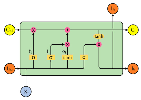
Figure 3.
LSTM structure diagram.
As presented in Figure 3, LSTM networks introduce three “gate” control units—the forgetting gate , the input gate , and the output gate — and an input unit . The three gate structures constitute LSTM’s unique “forgetting” process to regulate information flow, which is an advantage over traditional RNNs. This structure allows LSTM to recall long-distance information, effectively overcoming the vanishing gradient and making LSTM powerful for handling nonlinear sequence data with long- and short-term dependencies. In addition, compared to other machine learning methods, LSTM uses backpropagation through time, operating sequentially to better handle time series data. Since WS prediction involves temporal dependencies, LSTM can capture these relationships to accurately forecast future wind speeds over short time horizons. Consequently, LSTM has increasingly been applied to WS prediction tasks in recent years with good results. However, the performance of the LSTM model largely depends on the selection of its hyperparameters. Optimizing LSTM hyperparameters is a crucial step in applying the LSTM model. Choosing appropriate hyperparameters can effectively improve the model’s performance and generalization ability. Therefore, this paper will optimize the key parameters of LSTM, including the number of iterations Titer, learning rate LR, number of first-layer neurons L1, and number of second-layer neurons L2, using the MPOA with mean square error as the objective function.
2.4. VMD-MPOA–LSTM Combined Model
This section introduces a combined WS forecasting system of VMD-MPOA-LSTM based on time series preprocessing technology, a swarm intelligence optimization algorithm, and deep learning. It uses VMD to obtain the trend traits of the original WS sequence and MPOA to optimize LSTM hyperparameters. The framework of the VMD-MPOA-LSTM approach is illustrated in Figure 4, with the key steps described below.
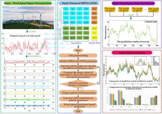
Figure 4.
The flowchart of VMD-MPOA-LSTM.
Step 1: Apply MPOA-VMD to decompose the original WS time series data. This takes sample entropy and RMSE as evaluation indexes, using the MPOA to obtain the optimal combination of K, alpha, and tau, improving reconstruction precision after decomposition. MPOA-VMD decomposes the time series into K IMFs while determining the optimal parameter group.
Step 2: use LSTM to predict each IMF component.
- (1)
- Split each of the K IMFs from decomposition into separate training and testing datasets;
- (2)
- Use the mean squared error between predicted and actual values as the objective function to optimize four LSTM hyperparameters;
- (3)
- Apply the optimized LSTM model to generate WS forecasts and the most accurate predicted values.
Step 3: aggregate the predicted values from each IMF through linear combination to yield the overall forecast for the original WS time series, obtaining the final result.
Step 4: evaluate the predictive performance of the proposed hybrid model using several evaluation indexes.
3. Experiment and Analysis Results
This section provides details on the dataset used, the evaluation metrics used to assess forecast accuracy, and the experimental setup and results for the application of the proposed combined VMD-MPOA-LSTM model.
3.1. Datasets
The original WS time series used in the experiments is from an eastern China wind farm. A total of 2600 data points were selected from 1 April 2021 at 0:00 to 28 April 2021 at 24:00 as the test data. The dataset was divided, with 2300 points allocated to the training set and 300 points to the testing set. The WS sampling interval was 15 min. Data from April were chosen because historical data show that average wind speeds in April are highest with frequent changes, better suiting model effectiveness validation. A 15 min resolution was selected because higher-resolution data have more peaks and complex noise, useful for verifying model performance, meeting China’s ultra-short-term forecasting requirements. Although 15 min sampling makes the data more unstable, decreasing prediction performance, it demonstrates data generality and makes the prediction more meaningful. Additionally, this study primarily focuses on ultra-short-term WS prediction. Due to the short sampling interval, WS data collected every 15 min can avoid the influence of seasonal factors. Therefore, the WS dataset no longer needed to be sampled separately for each season. Figure 5 displays a sample of the ultra-short-term WS data used in the experiments.
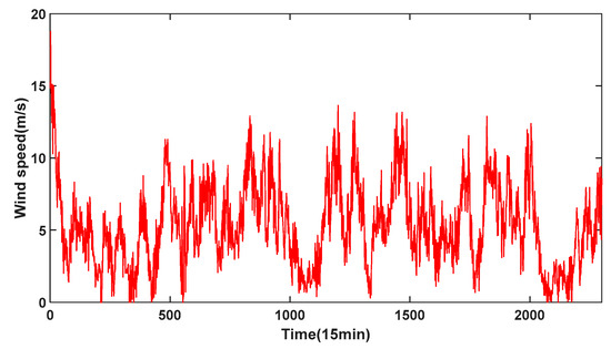
Figure 5.
Ultra-short-term WS data samples.
3.2. Performance Metrics
To thoroughly assess the model’s predictive capabilities, six common performance indicators were selected: MAE, RMSE, MAPE, R2, TIC, and EC. MAE, RMSE, and MAPE evaluate prediction accuracy. R2, TIC, and EC gauge model fit. The smaller the values for MAE, RMSE, MAPE, and TIC, and the larger the values for R2 and EC, the better the prediction performance. The specific expressions are as follows:
where represents the actual WS value at time ; represents the forecast value at time ; represents the average actual value; is the average forecast value; and N refers to the total number of data points in the time series .
Furthermore, the DM test [55] was employed to perform the validity analysis of the proposed model in this paper. The DM test utilizes the output statistic DM to judge whether there is a significant difference in the predictive capabilities of the two models.
3.3. Parameters Setting
In this paper, BP, SVM, ELM, LSTM, and their forecasting methods combined with some optimization algorithms are used for comparison with the proposed improved combined forecasting method. The parameter settings of PSO, MFO, WOA, POA, and MPOA are the same as in Table 4, except the population size is changed to eight and number of iterations to 50. The remaining model-related parameter settings are shown in Table 8. The models mentioned in this paper are named according to the primary methods adopted by each model. Models such as BP, ELM, and SVM are single models that do not use signal decomposition or optimization algorithms. Models like EMD-LSTM, VMD-LSTM, and EEMD-LSTM are combination models composed of various signal decomposition methods and LSTM. Models such as VMD-WOA-SVM, VMD-MPOA-SVM, VMD-WOA-LSTM, etc., are combination models that integrate the signal decomposition method VMD with swarm intelligence algorithms and single models.
Table 8.
The parameter values of each model.
3.4. Different Experiments and Result Analysis
Three experiments were conducted comparing the proposed model against other models. An analysis of the comparative results is provided in this section.
3.4.1. Experiment I: Comparison with Models Using Different Data Preprocessing Methods
To verify the effectiveness of the proposed MPOA-VMD signal decomposition method for WS prediction, it is compared with two common methods, EMD and EEMD. Figure 6 shows the MPOA-VMD WS signal decomposition results.
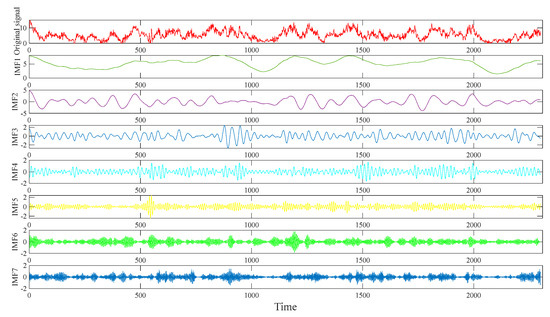
Figure 6.
VMD diagram of the original WS data.
Figure 7 displays the prediction results for the five models in this experiment. The proposed model is the improved VMD-MPOA-LSTM combined forecasting model studied in this paper. Table 9 shows the specific evaluation indicators for the prediction results of each combined model. Figure 8 depicts histograms comparing each evaluation index across models. Table 10 provides the DM test values between each model and the proposed model.
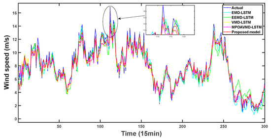
Figure 7.
The forecasting results of different models in Experiment I.
Table 9.
Evaluation index values of predicted results of different models in Experiment I.
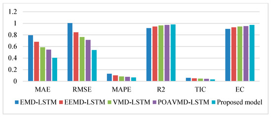
Figure 8.
Histogram of prediction results of different models in Experiment I.
Table 10.
The DM values of different models in Experiment I.
According to the WS prediction curves in Figure 7, the proposed model’s WS prediction values are closer to the actual values. This is reflected in its R2 performance index being the highest among the models. Moreover, Table 9 and Figure 8 show that the proposed model has better values across all six evaluation indicators compared to EMD-LSTM and EEMD-LSTM. This indicates that VMD is significantly more effective than EMD and EEMD for WS decomposition. Compared to VMD-LSTM, MPOAVMD-LSTM has slightly better results across the six indicators. This shows that MPOA optimization of VMD improves decomposition, enhancing model performance. The DM value represents the difference in the prediction sequence between the proposed combination model and other models, and its size represents the significance of the difference. All models in Table 10 exhibit DM values at a significance level of 10%, indicating a significant difference in the predictive performance of the proposed model compared to other models. The improvement in the model has led to a noticeable enhancement in predictive effectiveness. Overall, the examination of the five combined model results clearly demonstrates that the proposed model outperforms the others.
Remark: Examining the prediction results across six indicators shows that the proposed model demonstrates superior capabilities compared to the others. The DM test also reveals significant differences between the proposed model’s prediction sequences and those of the other models. It is evident that the introduction of decomposition methods can significantly improve the predictive performance of the ensemble model, and different decomposition methods yield distinctly different results in wind speed signal decomposition. Therefore, selecting an appropriate decomposition method is crucial for the wind speed prediction ensemble model. Additionally, the parameter settings of the decomposition method directly impact the quality of signal decomposition, thereby influencing the predictive performance of the model. Introducing optimization algorithms into the decomposition method for parameter optimization is beneficial for further enhancing the predictive performance of the ensemble model.
3.4.2. Experiment II: Comparison with Models Using Different Optimization Algorithms
To validate the efficacy of the MPOA for WS prediction, it is compared against combined models using conventional optimization algorithms, namely, PSO, WOA, MFO, and POA. Figure 9 displays the prediction results for the five different prediction models in this experiment. Table 11 provides the prediction results for each combined model. Figure 10 uses histograms to depict the values of each evaluation index applied to the prediction results across models.
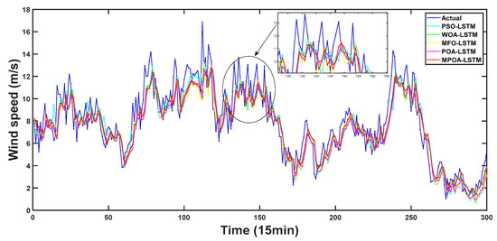
Figure 9.
The forecasting results of different models in Experiment II.
Table 11.
Evaluation index values of predicted results of different models in Experiment II.
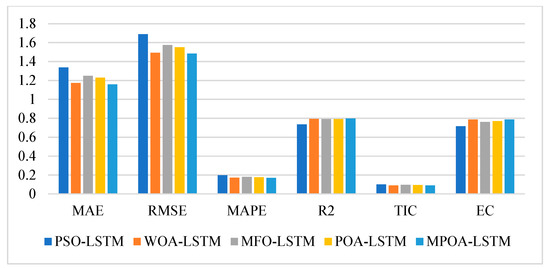
Figure 10.
Histogram of prediction results of different models in Experiment II.
In the above experiment, all five models used LSTM but with different optimization algorithms. Upon examination of the six evaluation index values presented in Table 11 and Figure 10, it can be observed that the prediction performance of the four models—WOA-LSTM, POA-LSTM, MFO-LSTM, and PSO-LSTM—decreases sequentially, and their MAPE values are 17.21%, 17.68%, 18.07%, and 19.76%, respectively. The prediction effect of WOA-LSTM is superior to that of the other three optimization algorithms. Furthermore, the six indicators of the combined model composed of MPOA and LSTM are better than those of WOA-LSTM, and its MAPE value is 16.92%. Therefore, it is proved that the MPOA not only further improves the optimization performance of POA, but also can enhance the prediction capabilities of LSTM more effectively than the other optimization algorithms.
Remark: Compared with the six prediction performance indicators of all models, it can be clearly seen that the optimization algorithm can enhance the prediction capabilities of the models to some degree, but the degree of improvement is very limited. In addition, it can be seen that the performance improvement in the POA for LSTM is not the best compared with other optimization algorithms. However, the optimization performance of the improved POA is significantly improved, which makes the prediction performance of MPOA-LSTM superior to that of other models.
3.4.3. Experiment Ⅲ: Comparison with Other Common Single and Combined Models
To further validate the efficacy of the proposed model, it was compared with five classical single forecasting models (ARIMA, BP, ELM, SVM, and LSTM) and six combined models (WOA-SVM, VMD-MPOA-BP, VMD-MPOA-ELM, VMD-WOA-SVM, VMD-MPOA-SVM, and VMD-WOA-LSTM). Figure 11 shows the prediction results of all predictive models in this experiment. Table 12 presents the specific evaluation index values of each combination model. Figure 12 depicts histograms of each evaluation index, comparing the prediction results of the different combined models. Table 13 indicates the DM values between each model and the proposed model.
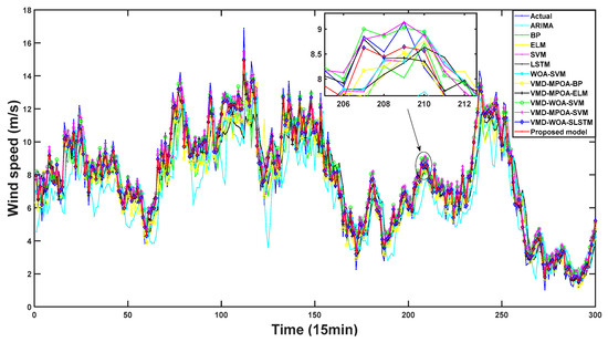
Figure 11.
The forecasting results of different models in Experiment III.
Table 12.
Evaluation index values of predicted results of different models in Experiment III.
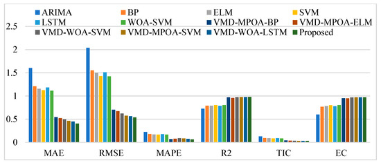
Figure 12.
Histogram of prediction results of different models in Experiment III.
Table 13.
The DM values of different models in Experiment III.
As shown in Table 12 and Figure 12, the evaluation indicators of the seven combined prediction models (WOA-SVM, VMD-MPOA-BP, VMD-MPOA-ELM,VMD-WOA-SVM,VMD-MPOA-SVM, VMD-WOA-LSTM, and the proposed model) are significantly better than those of the five single prediction models (ARIMA, BP, ELM, SVM, and LSTM). Moreover, the six combined forecasting models, VMD-MPOA-BP, VMD-MPOA-ELM, VMD-WOA-SVM, VMD-MPOA-SVM, VMD-WOA-LSTM, and the proposed model, which incorporate the signal decomposition method, an optimization algorithm, and machine learning, all demonstrate good prediction performance. Specifically, their MAPE values are 7.38%, 7.96%, 9.01%, 8.63%, 7.86%, and 6.49%, while their R2 values are 0.9726, 0.9585, 0.9756, 0.9779, 0.9781, and 0.9803, respectively. In conjunction with Figure 11, these results indicate that the proposed model possesses the best predictive capabilities among all the examined models.
4. Discussion
In this section, the predictive performance of each model type, the efficacy of the proposed model, and the enhancements in predictive accuracy as well as its performance in multi-step forecasting are discussed.
4.1. Comparison of Prediction Effects of Various Models
At present, the common combined model is a combination of an algorithm and prediction model, where the algorithm can be divided into decomposition methods and optimization algorithms. These can be paired with models individually or simultaneously. A decomposition method or optimization algorithm may be coupled with a model, or both algorithm types can be combined with a model concurrently. Based on the results of the three experiments presented in the previous section, the combined model demonstrates significantly better predictive performance compared to the single models. However, in a comparison of the experimental results of Experiment I and Experiment II, the results illustrate that while optimization algorithms are able to enhance a model’s prediction performance to some degree, the improvement is far less than that in the decomposition methods. Specifically, the evaluation indices of each model in Experiment I are markedly superior to those in Experiment II. For instance, the R2 values of each model in Experiment II were above 0.9, much higher than the R2 values of each model in Experiment I. Furthermore, the MAPE values in Experiment II were all below 13%, much lower than the MAPE values in Experiment I. This is because in AI-based WS prediction models, the processing of the original WS data has become one of the most crucial factors impacting the prediction capabilities of the model. Additionally, through a comparison of the results of Experiment III with those of Experiment I and Experiment II, it can be concluded that the combined model composed of decomposition methods, optimization algorithms, and a prediction model demonstrates the optimal predictive performance among all combination approaches examined. This combination approach can effectively utilize the advantages of decomposition methods and optimization algorithms to boost the performance of a single model. Overall, the model prediction effects of the various combination techniques are ranked in descending order as follows: (1) decomposition method, optimization algorithm, and single model; (2) decomposition method and single model; (3) optimization algorithm and single model; and (4) single model.
4.2. Effectiveness of the Proposed Model
The DM test was utilized in this paper to validate the efficacy of the proposed model, where the DM value signifies the divergence in predicted series between the proposed model and other models. Table 10 and Table 13 illustrate that only the VMD-WOA-SVM combined model has a DM value of 1.8611, which is at the 10% significance level, while the other models exhibit DM values at the 1% significance level. Therefore, the above results demonstrate that the prediction sequence generated by the proposed model significantly diverges from the sequences produced by the alternative models. This signifies that the predictive performance of the proposed model is markedly superior to that of the other examined models.
4.3. Improvement in the Prediction Performance of the Proposed Model
To evaluate the enhancement in predictive performance attained by the proposed model in a more comprehensive and intuitive manner, the six evaluation indicators mentioned in the previous section were utilized for an extensive comparison. The six indicator values for the proposed model were compared against those of all models across the three experiments, and the growth percentages of the evaluation index values between the proposed model and the other models are presented in Table 14. Taking PMAE as an example, its definition is
where MAE1 is the MAE value of the proposed model, and MAE2 is the MAE value of the comparison model.
Table 14.
Improvement percentage of the proposed model.
As depicted in Table 14, the six indicators of the proposed model outperform those of the other 20 prediction models examined in this paper. Among these, the maximum values of PMAE, PRMSE, PMAPE, PR2, PTIC, and PEC are 74.73%, 73.56%, 70.95%, 35.06%, 75.33%, and 65.41%, respectively, while their lowest values are 10.05%, 4.62%, 11.90%, 0.22%, 0.62%, and 0.02%, respectively. Therefore, the proposed model demonstrates outstanding predictive capabilities and robustness compared to all other models. Relative to the other models, the proposed model is markedly superior in each index, owing to the introduction of the improved POA. The enhanced POA can exert prominent optimization effects during the optimization of key VMD parameters and LSTM hyperparameter optimization. This enables the effective integration of the POA, VMD, and LSTM.
4.4. Effectiveness of Multi-Step Prediction
To examine the multi-step prediction capabilities of the proposed model, this section conducts simulation experiments of one-step-, two-step-, and three-step-ahead predictions for representative models discussed in Section 3. The experimental results are presented in Table 15. The values in bold in Table 15 denote the lowest MAE, RMSE, and MAPE values among the models. Additionally, the results in Table 15 illustrate that the one-step prediction performance is superior to the two-step and three-step predictions, indicating that prediction accuracy decreases as the number of predicted steps increases. Compared to the other four models, the proposed model demonstrates the optimal prediction performance at all step sizes. This signifies that the proposed model possesses superior multi-step prediction capabilities.
Table 15.
The simulation results of further step forecasting.
5. Conclusions
Wind power generation technology has been rapidly advancing, leading to increases in installed wind power capacity and its contribution to overall power supply. Hence, the impact of wind farms on reliable grid operation is becoming increasingly pronounced. However, the strong time variation in, nonlinearity of, and complexity of WS render the prediction effect unsatisfactory. Therefore, this paper proposes a combined ultra-short-term WS forecasting model utilizing a modified pelican optimization algorithm, composed of the WS decomposition methods VMD, MPOA, and LSTM. Firstly, techniques including tent map-based population initialization and Lévy flight strategy are introduced to form an improved POA, whose superior optimization performance is verified by comparison with other popular optimization algorithms. Secondly, given the difficulty in selecting the objective function in current VMD parameter optimization, the optimal number of decompositions in VMD is determined by the minimum sample entropy value. Concurrently, taking RSME as the objective function, the optimal parameter combination of k, alpha, and tau in VMD is obtained through the MPOA, effectively enhancing the accuracy of VMD signal reconstruction after WS signal decomposition. Additionally, the MPOA is applied to LSTM hyperparameter optimization to attain the optimal combination. Finally, single-month WS data from an eastern China wind farm were selected, where WS fluctuations during this month were most frequent and drastic compared to during other months of the year. The proposed combined prediction model is compared, analyzed, and evaluated against other models through the aforementioned three experiments and six evaluation indicators. The experiments focus on the quantitative analysis of utilizing optimization algorithms and decomposition methods to enhance the prediction capabilities of the combined model, providing a theoretical basis and practical guidance for constructing hybrid models moving forward. The experimental results demonstrate that the combined model achieves a MAPE of 6.49% and R2 of 0.9803, with optimal values on other metrics. This signifies that the combined model possesses superior predictive capabilities compared to conventional single models and earlier combined models. Additionally, through further, concurrent optimization of the parameters of both the decomposition method and the single model, the optimization algorithm, decomposition method, and single model can be organically integrated, markedly improving the WS predictive capabilities of the combined model. This study provides an effective approach to further enhance the predictive capabilities of combined models.
In future work, the following issues should be studied further:
- (1)
- The combination of an optimization algorithm, decomposition method, and neural network needs to be further studied based on the mechanism, and effective methods to realize the in-depth integration of different technologies need to be explored. At the same time, it is necessary to integrate more and more advanced technologies into the combination forecasting model to further enhance the predictive capabilities of the combination model;
- (2)
- Despite experimental verification of its superior predictive performance, a key limitation of the current model is its prolonged computation time. Reducing calculation time and improving forecasting efficiency should be priority research directions moving forward. Parallel computing, algorithm optimization, model simplification, and data preprocessing will likely be effective solutions to reduce computation time and improve the computational efficiency of the combined model;
- (3)
- The model predicts WS through historical data and only considers the magnitude of WS. In fact, meteorological parameters like wind orientation, temperature, moisture, and barometric pressure impact the precision of predictions. In the future, it is necessary to consider combining these external factors to establish a multi-input prediction model for further enhancing WS forecasting accuracy;
- (4)
- The proposed model will be tested in additional actual wind farm scenarios and compared with more prediction models to further validate its robustness and adaptability;
- (5)
- For the MPOA, although the improvement methods and experimental validation results are detailed, there is a lack of theoretical analysis of the improved algorithm. A mathematical proof of the convergence of the improved algorithm and the analysis of the mechanisms that enhance the model’s prediction performance will be important directions for future research.
Author Contributions
Conceptualization, L.G. and C.X.; methodology, L.G.; validation, X.A. and X.H.; formal analysis, L.G.; investigation, C.X.; resources, L.G. and X.H.; data curation, X.A.; writing—original draft preparation, L.G.; writing—review and editing, F.X.; supervision, X.A.; project administration, X.H.; funding acquisition, L.G., X.H. and C.X. All authors have read and agreed to the published version of the manuscript.
Funding
This work was supported by the National Natural Science Foundation of China (No. 52406234), the China Postdoctoral Science Foundation (No. 2024M760739), the Fundamental Research Funds for the Central Universities (No. B240201171), the Changzhou Science and Technology Plan—Applied Basic Research Special Project (No. CJ20240094), and the National Key R&D Plan of China (No. 2024YFE0212200).
Institutional Review Board Statement
Not applicable.
Informed Consent Statement
Not applicable.
Data Availability Statement
The data that support this manuscript are available from Chang Xu upon reasonable request.
Conflicts of Interest
The authors declare no conflicts of interest.
Abbreviations
The following abbreviations are used in this manuscript:
| WS | wind speed |
| NWP | numerical weather prediction |
| MA | moving average |
| ARMA | autoregressive moving average |
| ARIMA | autoregressive integrated moving average |
| POA | pelican optimization algorithm |
| MPOA | modified pelican optimization algorithm |
| PSO | particle swarm optimization |
| MFO | moth–flame optimization |
| WOA | whale optimization algorithm |
| DA | dragonfly algorithm |
| GWO | grey wolf optimization |
| EMD | empirical mode decomposition |
| EEMD | ensemble empirical mode decomposition |
| VMD | variational mode decomposition |
| CEEMD | complementary ensemble empirical mode decomposition |
| LSTM | long short-term memory |
| RNN | recurrent neural network |
| BP | backpropagation |
| ELM | extreme learning machine |
| SVM | support vector machine |
| CNN | convolutional neural network |
| RNN | recurrent neural network |
| DBN | deep belief network |
| AI | artificial intelligence |
| ENN | evolutionary neural network |
| GRNN | generalized regression neural network |
| ARAR | autoregressive–autoregressive |
| ANN | artificial neural network |
| IMF | intrinsic mode functions |
| MAE | mean absolute error |
| RMSE | root mean square error |
| MAPE | mean absolute percentile error |
| TIC | Theil’s inequality coefficient |
| EC | efficiency coefficient |
| DM | Diebold–Mariano |
References
- Yang, B.; Zhong, L.; Wang, J.; Shu, H.; Zhang, X.; Yu, T.; Sun, L. State-of-the-art one-stop handbook on wind forecasting technologies: An overview of classifications, methodologies, and analysis. J. Clean. Prod. 2021, 283, 124628. [Google Scholar] [CrossRef]
- GWEC. Global Wind Energy Council. Global Wind Report; GWEC: Brussels, Belgium, 2021. [Google Scholar]
- Badal, F.R.; Das, P.; Sarker, S.K.; Das, S.K. A survey on control issues in renewable energy integration and microgrid. Protect. Contr. Mod. Power Syst. 2019, 4, 6008. [Google Scholar] [CrossRef]
- Yang, B.; Zhang, X.; Yu, T.; Shu, H.; Fang, Z. Grouped grey wolf optimizer for maximum power point tracking of doubly-fed induction generator based wind turbine. Energy Convers. Manag. 2017, 133, 427–443. [Google Scholar] [CrossRef]
- Yuan, X.; Chen, C.; Yuan, Y.; Huang, Y.; Tan, Q. Short-term wind power prediction based on LSSVM-GSA model. Energy Convers. Manag. 2015, 101, 393–401. [Google Scholar] [CrossRef]
- Liu, T.; Liu, S.; Heng, J.; Gao, Y. A new hybrid approach for wind speed forecasting applying support vector machine with ensemble empirical mode decomposition and cuckoo search algorithm. Appl. Sci. 2018, 8, 1754. [Google Scholar] [CrossRef]
- Feng, S.; Wang, W.; Liu, C.; Dai, H. Short term wind speed predictionbase on physical principle. Acta Energiae Solaris Sin. 2011, 32, 611–616. [Google Scholar]
- Liu, Y.; Wang, Y.; Li, L.; Han, S.; Infield, D. Numerical weather prediction wind correction methods and its impact on computational fluid dynamics based wind power forecasting. J. Renew. Sustain. Energy 2016, 8, 033302. [Google Scholar] [CrossRef]
- Li, Y.; Tang, F.; Gao, X.; Zhang, T.; Qi, J.; Xie, J.; Li, X.; Guo, Y. Numerical Weather Prediction Correction Strategy for Short-Term Wind Power Forecasting Based on Bidirectional Gated Recurrent Unit and XGBoost. Front. Energy Res. 2022, 9, 836144. [Google Scholar] [CrossRef]
- Liu, Y.; Yi, S. Optimization of a wind power time series prediction model based on a two-parameter least squares support vector machine. J. Beijing Univ. Chem. Technol. 2019, 46, 97–102. [Google Scholar]
- Zheng, P.; Yu, L.; Hou, S.; Wang, C. Multi-Step Wind Power Forecasting based on Kalman Filter Modification. J. Eng. Therm. Energy Power 2020, 35, 235–241. [Google Scholar]
- Karakus, O.; Kuruoglu, E.E.; Altinkaya, M.A. One-day ahead wind speed/power prediction based on polynomial autoregressive model. IET Renew. Power Gen. 2017, 11, 1430–1439. [Google Scholar] [CrossRef]
- Riahy, G.H.; Abedi, M. Short term wind speed forecasting for wind turbine applications using linear prediction method. Renew. Energy 2008, 33, 35–41. [Google Scholar] [CrossRef]
- Do, D.P.N.; Lee, Y.; Choi, J. Hourly Average wind speed Simulation and Forecast Based on ARMA Model in Jeju Island, Korea. J. Electr. Eng. Technol. 2016, 11, 1548–1555. [Google Scholar] [CrossRef]
- Zuluaga, C.D.; Alvarez, M.A.; Giraldo, E. Short-term wind speed prediction based on robust Kalman filtering: An experimental comparison. Appl. Energy 2015, 156, 321–330. [Google Scholar] [CrossRef]
- Cheng, Z.; Wang, J. A new combined model based on multi-objective salp swarm optimization for wind speed forecasting. Appl. Soft Comput. 2020, 92, 106294. [Google Scholar] [CrossRef]
- Liu, M.; Cao, Z.; Zhang, J.; Wang, L.; Huang, C.; Luo, X. Short-term wind speed forecasting based on the Jaya-SVM model. Int. J. Electr. Power 2020, 121, 106056. [Google Scholar] [CrossRef]
- Arjun, B.; Kumar, G.; Sudhansu, K.M. A review of short term load forecasting using artifificial neural network models. Procedia Comput. Sci. 2015, 48, 121–125. [Google Scholar]
- Mehrkanoon, S. Deep shared representation learning for weather elements forecasting. Knowl. Based Syst. 2019, 179, 120–128. [Google Scholar] [CrossRef]
- Shi, Z.; Liang, H.; Dinavahi, V. Direct interval forecast of uncertain wind power based on recurrent neural networks. IEEE Trans. Sustain. Energy 2018, 9, 1177–1187. [Google Scholar] [CrossRef]
- Zhang, C.; Chen, C.; Gan, M.; Chen, L. Predictive deep boltzmann machine for multiperiod wind speed forecasting. IEEE Trans. Sustain. Energy 2015, 6, 1416–1425. [Google Scholar] [CrossRef]
- Wang, K.; Qi, X.; Liu, H.; Song, J. Deep belief network based k-means cluster approach for short-term wind power forecasting. Energy 2018, 165, 840–852. [Google Scholar] [CrossRef]
- Zhao, J.; Guo, Y.; Lin, Y.; Zhao, Z.; Guo, Z. A novel dynamic ensemble of numerical weather prediction for multi-step wind speed forecasting with deep reinforcement learning and error sequence modeling. Energy 2024, 32, 131787. [Google Scholar] [CrossRef]
- Zhu, L.; Lian, C.; Zeng, Z.; Su, Y. A broad learning system with ensemble and classification methods for multi-step-ahead wind speed prediction. Cogn. Comput. 2019, 12, 654–666. [Google Scholar] [CrossRef]
- Tascikaraoglu, A.; Uzunoglu, M. A review of combined approaches for prediction of short-term wind speed and power. Renew. Sustain. Energy Rev. 2014, 34, 243–254. [Google Scholar] [CrossRef]
- Neto, P.S.G.D.; Oliveira, J.F.L.; Santos, D.S.D.; Siqueira, H.V.; Marinho, M.H.N.; Madeiro, F. A hybrid nonlinear combination system for monthly wind speed forecasting. IEEE Access 2020, 8, 191365–191377. [Google Scholar] [CrossRef]
- Shahzad, M.N.; Kanwal, S.; Hussanan, A. A new hybrid ARAR and neural network model for multi-step ahead wind speed forecasting in three regions of pakistan. IEEE Access 2020, 8, 199382–199392. [Google Scholar] [CrossRef]
- Liang, C.; Liu, Y.; Zhou, J.; Yan, J.; Lu, Z. Wind speed prediction at multi-locations based on combination of recurrent and convolutional neural networks. Power Syst. Technol. 2021, 45, 534–542. [Google Scholar]
- Altan, A. Performance of metaheuristic optimization algorithms based on swarm intelligence in attitude and altitude control of unmanned aerial vehicle for path following. In Proceedings of the 4th International Symposium on Multidisciplinary Studies and Innovative Technologies, Istanbul, Turkey, 22–24 October 2020. [Google Scholar]
- Ozcelik, Y.B.; Altan, A. Overcoming nonlinear dynamics in diabetic retinopathy classification: A robust AI-based model with chaotic swarm intelligence optimization and recurrent long short-term memory. Fractal Fract. 2023, 7, 589. [Google Scholar] [CrossRef]
- Bou-Rabee, M.; Lodi, K.A.; Ali, M.; Ansari, M.F.; Tariq, M.; Sulaiman, S.A. One-month-ahead wind speed forecasting using hybrid AI model for coastal locations. IEEE Access 2020, 8, 198482–198493. [Google Scholar] [CrossRef]
- Hu, R.; Qiao, J.; Li, Y.; Sun, Y.; Wang, B. Medium and long term wind power forecast based on WOA-VMD-SSA-LSTM. Acta Energiae Solaris Sin. 2024, 45, 549–556. [Google Scholar]
- Li, L.; Zhao, X.; Tseng, M.L.; Tan, R. Short-term wind power forecasting based on support vector machine with improved dragonfly algorithm. J. Clean. Prod. 2020, 242, 118447. [Google Scholar] [CrossRef]
- Phan, Q.B.; Nguyen, T.T. Enhancing wind speed forecasting accuracy using a GWO-nested CEEMDAN-CNN-BiLSTM model. ICT Express 2024, 10, 485–490. [Google Scholar] [CrossRef]
- Xiong, Z.; Yao, J.; Huang, Y.; Yu, Z.; Liu, Y. A wind speed forecasting method based on EMD-MGM with switching QR loss function and novel subsequence superposition. Appl. Energy 2024, 353, 122248. [Google Scholar] [CrossRef]
- Parri, S.; Teeparthi, K. VMD-SCINet: A hybrid model for improved wind speed forecasting. Earth SCI Inform. 2024, 17, 329–350. [Google Scholar] [CrossRef]
- Shang, Z.; Chen, Y.; Chen, Y.; Guo, Z.; Yang, Y. Decomposition-based wind speed forecasting model using causal convolutional network and attention mechanism. Expert Syst. Appl. 2023, 223, 119878. [Google Scholar] [CrossRef]
- Chen, J.; Guo, Z.; Zhang, L.; Zhang, S. Short-term wind speed prediction based on improved Hilbert-Huang transform method coupled with NAR dynamic neural network model. Sci. Rep. 2024, 14, 617. [Google Scholar] [CrossRef]
- Ibrahim, A.; Mirjalili, S.; El-Said, M.; Ghoneim, S.S.M.; Al-Harthi, M.M.; Ibrahim, T.F.; El-Kenawy, E.M. Wind speed ensemble forecasting based on deep learning using adaptive dynamic optimization algorithm. IEEE Access 2021, 9, 125787–125804. [Google Scholar] [CrossRef]
- Altan, A.; Karasu, S.; Zio, E. A new hybrid model for wind speed forecasting combining long short-term memory neural network, decomposition methods and grey wolf optimizer. Appl. Soft Comput. 2021, 100, 106996. [Google Scholar] [CrossRef]
- Trojovsky, P.; Dehghani, M. Pelican Optimization algorithm: A novel nature-inspired algorithm for engineering applications. Sensors 2022, 22, 855. [Google Scholar] [CrossRef]
- Kaur, G.; Arora, S. Chaotic whale optimization algorithm. J. Comput. Des. Eng. 2018, 5, 275–284. [Google Scholar] [CrossRef]
- Arora, S.; Sharma, M.; Anand, P. A Novel Chaotic Interior Search Algorithm for Global Optimization and Feature Selection. Appl. Artif. Intell. 2020, 34, 292–328. [Google Scholar] [CrossRef]
- Dragomiretskiy, K.; Zosso, D. Variational Mode Decomposition. IEEE Trans. Signal Process. 2014, 62, 531–544. [Google Scholar] [CrossRef]
- Gai, J.; Shen, J.; Hu, Y.; Wang, H. An integrated method based on hybrid grey wolf optimizer improved variational mode decomposition and deep neural network for fault diagnosis of rolling bearing. Measurement 2020, 162, 107901. [Google Scholar] [CrossRef]
- Xu, H.; Lu, T.; Montillet, J.P.; He, X. An improved adaptive IVMD-WPT-based noise reduction algorithm on GPS height time series. Sensors 2022, 21, 8295. [Google Scholar] [CrossRef] [PubMed]
- Richman, J.S.; Moorman, J.R. Physiological time-series analysis using approximate entropy and sample entropy. Am. J. Physiol. Heart Circ. Physiol. 2000, 278, 2039–2049. [Google Scholar] [CrossRef]
- Hochreiter, S.; Schmidhuber, J. Long short-term memory. Neural Comput. 1997, 9, 1735–1780. [Google Scholar] [CrossRef]
- Alamri, N.M.H.; Packianather, M.; Bigot, S. Optimizing the Parameters of Long Short-Term Memory Networks Using the Bees Algorithm. Appl. Sci. 2023, 13, 2536. [Google Scholar] [CrossRef]
- Subbiah, S.S.; Paramasivan, S.K.; Arockiasamy, K.; Senthivel, S.; Thangavel, M. Deep learning for wind speed forecasting using bi-lstm with selected features. Intell. Autom. Soft Comput. 2023, 35, 3824–3829. [Google Scholar]
- Wang, Y.; Vijayakumar, P.; Gupta, B.B.; Alhalabi, W.; Sivaraman, A. An improved entity recognition approach to cyber social knowledge provision of intellectual property using a CRF-LSTM model. Pattern Recogn. Lett. 2022, 163, 145–151. [Google Scholar] [CrossRef]
- Li, S.; Qin, D.; Wu, X.; Li, J.; Li, B.; Han, W. False Alert Detection Based on Deep Learning and Machine Learning. Int. J. Semant. Web Inf. Syst. 2022, 18, 297035. [Google Scholar] [CrossRef]
- Akl, N.A.; Khoury, J.E.; Mansour, C. Trip-based prediction of hybrid electric vehicles velocity using artifificial neural networks. In Proceedings of the 2021 IEEE 3rd International Multidisciplinary Conference on Engineering Technology (IMCET), Beirut, Lebanon, 8–10 December 2021; pp. 60–65. [Google Scholar]
- Ehteram, M.; Ahmed, A.N.; Khozani, Z.S.; El-Shafie, A. Graph convolutional network-Long short term memory neural network- multi layer perceptron- Gaussian progress regression model: A new deep learning model for predicting ozone concertation. Atmos. Pollut. Res. 2023, 14, 101766. [Google Scholar] [CrossRef]
- Diebold, F.X.; Mariano, R.S. Comparing predictive accuracy. J. Bus. Econ. Stat. 1995, 13, 134–144. [Google Scholar] [CrossRef]
Disclaimer/Publisher’s Note: The statements, opinions and data contained in all publications are solely those of the individual author(s) and contributor(s) and not of MDPI and/or the editor(s). MDPI and/or the editor(s) disclaim responsibility for any injury to people or property resulting from any ideas, methods, instructions or products referred to in the content. |
© 2025 by the authors. Licensee MDPI, Basel, Switzerland. This article is an open access article distributed under the terms and conditions of the Creative Commons Attribution (CC BY) license (https://creativecommons.org/licenses/by/4.0/).