
Assessing Carbon Emissions’ Impact on Drought in China’s Arid Regions: Cross-Lagged and Spatial Models


Abstract
1. Introduction
2. Materials and Methods
2.1. Data Source
2.2. Theory and Calculation
2.2.1. Carbon Emission
2.2.2. Random Intercept Cross-Lagged Panel Model and Traditional Cross-Lagged Panel Model
2.2.3. Spatial Econometrics
3. Results
3.1. Descriptive Statistics of the Variables
3.2. Results of the Random Intercept Cross-Lagged Model
3.3. Spatial Econometric Analysis Results
3.4. Robustness Test
3.4.1. Replace the Spatial Weight Matrix
3.4.2. Divide into Different Time Periods
4. Discussion
5. Conclusions
Supplementary Materials
Author Contributions
Funding
Institutional Review Board Statement
Informed Consent Statement
Data Availability Statement
Acknowledgments
Conflicts of Interest
Abbreviations
| RI-CLPM | Random Intercept Cross-Lagged Panel Model |
| CLPM | Cross-Lagged Panel Model |
| SDM | Spatial Durbin Model |
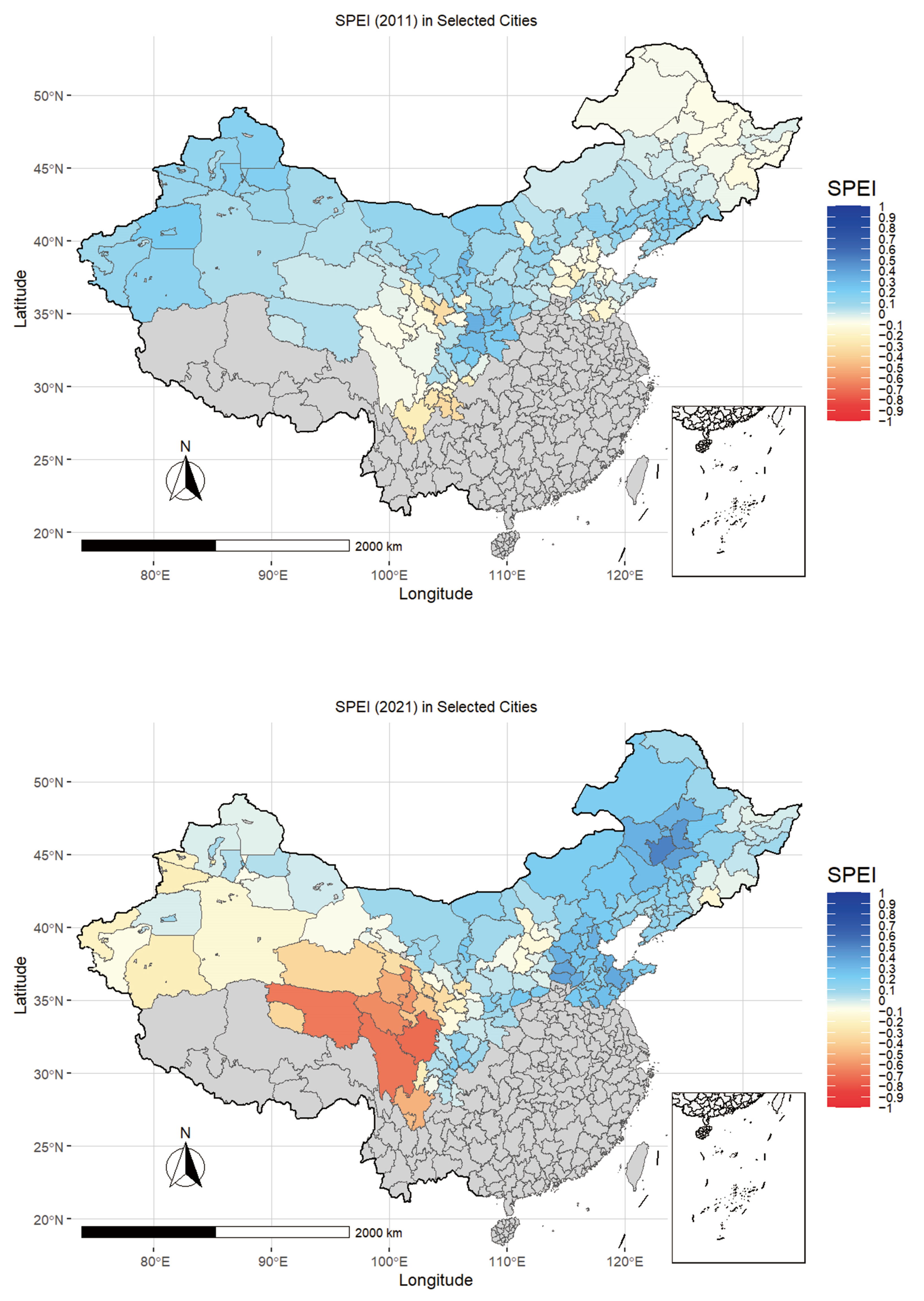
| SPEI | Standardized Precipitation Evapotranspiration Index |
| ln(Carbon) | Take the logarithm of the carbon emission data for prefecture-level cities |
| ln(Pop) | The logarithm of population density |
| Ext_Wea | The proportion of extremely cold and extremely hot days |
| Ind_Str | The degree of urbanization (the ratio of tertiary industry GDP to secondary industry GDP) |
| H-H | High–High, where both local and neighboring values exceed the mean |
| L-L | Low–Low, where both local and neighboring values are below the mean |
| H-L | High–Low, where local values are above the mean while neighboring values are below |
| L-H | Low–High, where local values are below the mean while neighboring values are above |
Appendix A

| Types of Tests | Pooling | Space Fixed | Time Fixed | Space–Time Fixed |
|---|---|---|---|---|
| LM-lag | 23.513 *** | 48.807 *** | 3.9052 ** | 16.447 *** |
| LM-error | 26.691 *** | 46.958 *** | 1.0484 | 11.449 *** |
| robust LM-lag | 0.0870 | 1.9785 | 8.658 *** | 11.288 *** |
| robust LM-error | 3.2648 * | 0.1297 | 5.8012 ** | 6.2894 ** |
| Types of Tests | Chi-Square Statistic (Degrees of Freedom) | p-Value |
|---|---|---|
| Hausman | 22.95 (5) | 0.0003 |
| Wald_lag | 23.80 (7) | 0.0012 |
| Wald_error | 10.29 (7) | 0.1730 |
| LR_lag | 23.19 (7) | 0.0016 |
| LR_error | 10.11 (7) | 0.1826 |
| Model | R-Squared | Adjusted R-Squared | Akaike Information Criterion |
|---|---|---|---|
| Linear | 0.7569634 | 0.7395539 | 3426.9352 |
| Logarithmic | 0.5518169 | 0.519712 | 3656.4314 |
| Exponential | 0.5818566 | 0.5519036 | −496.5862 |
| Power | 0.8558181 | 0.8454899 | −895.8669 |
| Sample_Size | Time_Points | ICC | Errors | Not_Converged | Inadmissible | Population_Value | Average | Minimum | SD | SEAvg | MSE | Accuracy | Coverage | Power |
|---|---|---|---|---|---|---|---|---|---|---|---|---|---|---|
| 160 | 5 | 0.1 | 0 | 0 | 303 | 0.2 | 0.196 | −0.122 | 0.09 | 0.088 | 0.008 | 0.24 | 0.659 | 0.43 |
| 170 | 5 | 0.1 | 0 | 0 | 289 | 0.2 | 0.194 | −0.081 | 0.088 | 0.085 | 0.008 | 0.238 | 0.669 | 0.457 |
| 180 | 5 | 0.1 | 0 | 0 | 295 | 0.2 | 0.195 | −0.086 | 0.083 | 0.083 | 0.007 | 0.229 | 0.667 | 0.457 |
| 190 | 5 | 0.1 | 0 | 0 | 241 | 0.2 | 0.192 | −0.118 | 0.083 | 0.08 | 0.007 | 0.238 | 0.724 | 0.497 |
| 200 | 5 | 0.1 | 0 | 0 | 259 | 0.2 | 0.194 | −0.048 | 0.08 | 0.079 | 0.006 | 0.229 | 0.702 | 0.509 |
| 160 | 10 | 0.1 | 0 | 0 | 31 | 0.2 | 0.2 | −0.097 | 0.083 | 0.081 | 0.007 | 0.309 | 0.924 | 0.658 |
| 170 | 10 | 0.1 | 0 | 0 | 24 | 0.2 | 0.201 | −0.084 | 0.078 | 0.079 | 0.006 | 0.3 | 0.926 | 0.719 |
| 180 | 10 | 0.1 | 0 | 0 | 25 | 0.2 | 0.202 | −0.019 | 0.077 | 0.076 | 0.006 | 0.291 | 0.925 | 0.74 |
| 190 | 10 | 0.1 | 0 | 0 | 14 | 0.2 | 0.201 | −0.005 | 0.073 | 0.074 | 0.005 | 0.286 | 0.94 | 0.764 |
| 200 | 10 | 0.1 | 0 | 0 | 12 | 0.2 | 0.2 | −0.008 | 0.071 | 0.072 | 0.005 | 0.279 | 0.933 | 0.796 |
| 160 | 15 | 0.1 | 0 | 0 | 0 | 0.2 | 0.201 | −0.025 | 0.082 | 0.08 | 0.007 | 0.312 | 0.943 | 0.702 |
| 170 | 15 | 0.1 | 0 | 0 | 1 | 0.2 | 0.2 | −0.069 | 0.081 | 0.077 | 0.007 | 0.303 | 0.934 | 0.717 |
| 180 | 15 | 0.1 | 0 | 0 | 5 | 0.2 | 0.201 | −0.019 | 0.076 | 0.075 | 0.006 | 0.293 | 0.938 | 0.747 |
| 190 | 15 | 0.1 | 0 | 0 | 3 | 0.2 | 0.195 | −0.031 | 0.075 | 0.073 | 0.006 | 0.285 | 0.944 | 0.758 |
| 200 | 15 | 0.1 | 0 | 0 | 1 | 0.2 | 0.202 | −0.065 | 0.072 | 0.071 | 0.005 | 0.279 | 0.952 | 0.803 |
| 160 | 5 | 0.3 | 0 | 0 | 7 | 0.2 | 0.196 | −0.146 | 0.098 | 0.096 | 0.01 | 0.374 | 0.933 | 0.526 |
| 170 | 5 | 0.3 | 0 | 0 | 4 | 0.2 | 0.2 | −0.144 | 0.097 | 0.093 | 0.009 | 0.362 | 0.935 | 0.603 |
| 180 | 5 | 0.3 | 0 | 0 | 6 | 0.2 | 0.199 | −0.107 | 0.092 | 0.09 | 0.009 | 0.352 | 0.931 | 0.6 |
| 190 | 5 | 0.3 | 0 | 0 | 8 | 0.2 | 0.201 | −0.149 | 0.094 | 0.087 | 0.009 | 0.34 | 0.936 | 0.629 |
| 200 | 5 | 0.3 | 0 | 0 | 1 | 0.2 | 0.204 | −0.051 | 0.09 | 0.086 | 0.008 | 0.337 | 0.942 | 0.66 |
| 160 | 10 | 0.3 | 0 | 0 | 0 | 0.2 | 0.199 | −0.089 | 0.086 | 0.085 | 0.007 | 0.335 | 0.942 | 0.665 |
| 170 | 10 | 0.3 | 0 | 0 | 0 | 0.2 | 0.2 | −0.103 | 0.088 | 0.083 | 0.008 | 0.326 | 0.937 | 0.656 |
| 180 | 10 | 0.3 | 0 | 0 | 0 | 0.2 | 0.202 | −0.093 | 0.083 | 0.081 | 0.007 | 0.317 | 0.946 | 0.707 |
| 190 | 10 | 0.3 | 0 | 0 | 0 | 0.2 | 0.201 | −0.016 | 0.079 | 0.079 | 0.006 | 0.309 | 0.941 | 0.718 |
| 200 | 10 | 0.3 | 0 | 0 | 0 | 0.2 | 0.2 | −0.073 | 0.082 | 0.077 | 0.007 | 0.3 | 0.939 | 0.739 |
| 160 | 15 | 0.3 | 0 | 0 | 0 | 0.2 | 0.199 | −0.053 | 0.086 | 0.082 | 0.007 | 0.323 | 0.928 | 0.672 |
| 170 | 15 | 0.3 | 0 | 0 | 0 | 0.2 | 0.199 | −0.033 | 0.082 | 0.08 | 0.007 | 0.314 | 0.946 | 0.697 |
| 180 | 15 | 0.3 | 0 | 0 | 0 | 0.2 | 0.196 | −0.087 | 0.08 | 0.078 | 0.006 | 0.305 | 0.942 | 0.709 |
| 190 | 15 | 0.3 | 0 | 0 | 0 | 0.2 | 0.201 | −0.034 | 0.077 | 0.076 | 0.006 | 0.297 | 0.946 | 0.763 |
| 200 | 15 | 0.3 | 0 | 0 | 0 | 0.2 | 0.198 | −0.054 | 0.074 | 0.074 | 0.005 | 0.29 | 0.949 | 0.752 |
| 160 | 5 | 0.5 | 0 | 0 | 0 | 0.2 | 0.202 | −0.208 | 0.11 | 0.106 | 0.012 | 0.417 | 0.937 | 0.492 |
| 170 | 5 | 0.5 | 0 | 0 | 0 | 0.2 | 0.2 | −0.176 | 0.107 | 0.104 | 0.011 | 0.406 | 0.95 | 0.51 |
| 180 | 5 | 0.5 | 0 | 0 | 0 | 0.2 | 0.201 | −0.137 | 0.101 | 0.101 | 0.01 | 0.394 | 0.955 | 0.534 |
| 190 | 5 | 0.5 | 0 | 0 | 0 | 0.2 | 0.199 | −0.141 | 0.102 | 0.097 | 0.01 | 0.382 | 0.943 | 0.545 |
| 200 | 5 | 0.5 | 0 | 0 | 0 | 0.2 | 0.199 | −0.118 | 0.101 | 0.095 | 0.01 | 0.373 | 0.935 | 0.545 |
| 160 | 10 | 0.5 | 0 | 0 | 0 | 0.2 | 0.199 | −0.168 | 0.092 | 0.089 | 0.008 | 0.348 | 0.953 | 0.599 |
| 170 | 10 | 0.5 | 0 | 0 | 0 | 0.2 | 0.2 | −0.085 | 0.09 | 0.087 | 0.008 | 0.34 | 0.951 | 0.637 |
| 180 | 10 | 0.5 | 0 | 0 | 0 | 0.2 | 0.202 | −0.116 | 0.089 | 0.084 | 0.008 | 0.329 | 0.942 | 0.665 |
| 190 | 10 | 0.5 | 0 | 0 | 0 | 0.2 | 0.198 | −0.058 | 0.085 | 0.081 | 0.007 | 0.319 | 0.948 | 0.671 |
| 200 | 10 | 0.5 | 0 | 0 | 0 | 0.2 | 0.198 | −0.073 | 0.081 | 0.079 | 0.007 | 0.311 | 0.943 | 0.704 |
| 160 | 15 | 0.5 | 0 | 0 | 0 | 0.2 | 0.2 | −0.125 | 0.09 | 0.084 | 0.008 | 0.33 | 0.94 | 0.657 |
| 170 | 15 | 0.5 | 0 | 0 | 0 | 0.2 | 0.199 | −0.089 | 0.084 | 0.081 | 0.007 | 0.319 | 0.95 | 0.674 |
| 180 | 15 | 0.5 | 0 | 0 | 0 | 0.2 | 0.198 | −0.106 | 0.08 | 0.08 | 0.006 | 0.313 | 0.951 | 0.695 |
| 190 | 15 | 0.5 | 0 | 0 | 0 | 0.2 | 0.2 | −0.03 | 0.077 | 0.077 | 0.006 | 0.302 | 0.951 | 0.739 |
| 200 | 15 | 0.5 | 0 | 0 | 0 | 0.2 | 0.199 | −0.034 | 0.075 | 0.075 | 0.006 | 0.295 | 0.947 | 0.742 |
| 160 | 5 | 0.7 | 0 | 0 | 1 | 0.2 | 0.199 | −0.245 | 0.128 | 0.125 | 0.016 | 0.488 | 0.95 | 0.41 |
| 170 | 5 | 0.7 | 0 | 0 | 0 | 0.2 | 0.192 | −0.336 | 0.127 | 0.121 | 0.016 | 0.474 | 0.946 | 0.372 |
| 180 | 5 | 0.7 | 0 | 0 | 0 | 0.2 | 0.194 | −0.269 | 0.128 | 0.118 | 0.016 | 0.463 | 0.933 | 0.416 |
| 190 | 5 | 0.7 | 0 | 0 | 0 | 0.2 | 0.203 | −0.297 | 0.123 | 0.114 | 0.015 | 0.447 | 0.934 | 0.471 |
| 200 | 5 | 0.7 | 0 | 0 | 0 | 0.2 | 0.199 | −0.2 | 0.117 | 0.11 | 0.014 | 0.432 | 0.947 | 0.472 |
| 160 | 10 | 0.7 | 0 | 0 | 0 | 0.2 | 0.2 | −0.117 | 0.093 | 0.092 | 0.009 | 0.359 | 0.95 | 0.602 |
| 170 | 10 | 0.7 | 0 | 0 | 0 | 0.2 | 0.197 | −0.182 | 0.095 | 0.089 | 0.009 | 0.349 | 0.934 | 0.595 |
| 180 | 10 | 0.7 | 0 | 0 | 0 | 0.2 | 0.198 | −0.094 | 0.09 | 0.086 | 0.008 | 0.338 | 0.947 | 0.626 |
| 190 | 10 | 0.7 | 0 | 0 | 0 | 0.2 | 0.203 | −0.139 | 0.087 | 0.084 | 0.008 | 0.329 | 0.945 | 0.673 |
| 200 | 10 | 0.7 | 0 | 0 | 0 | 0.2 | 0.199 | −0.043 | 0.083 | 0.082 | 0.007 | 0.321 | 0.946 | 0.679 |
| 160 | 15 | 0.7 | 0 | 0 | 0 | 0.2 | 0.202 | −0.053 | 0.087 | 0.085 | 0.008 | 0.333 | 0.947 | 0.679 |
| 170 | 15 | 0.7 | 0 | 0 | 0 | 0.2 | 0.203 | −0.084 | 0.088 | 0.083 | 0.008 | 0.324 | 0.94 | 0.695 |
| 180 | 15 | 0.7 | 0 | 0 | 0 | 0.2 | 0.199 | −0.107 | 0.084 | 0.08 | 0.007 | 0.313 | 0.932 | 0.695 |
| 190 | 15 | 0.7 | 0 | 0 | 0 | 0.2 | 0.203 | −0.019 | 0.078 | 0.078 | 0.006 | 0.306 | 0.962 | 0.735 |
| 200 | 15 | 0.7 | 0 | 0 | 0 | 0.2 | 0.2 | −0.062 | 0.077 | 0.076 | 0.006 | 0.298 | 0.944 | 0.75 |
| Regressions | Estimate | Std. Err | z-Value | p-Value |
|---|---|---|---|---|
| wc2~wc1 | 0.954 | 0.016 | 60.885 | 0 |
| wc2~ws1 | −0.049 | 0.064 | −0.764 | 0.445 |
| ws2~wc1 | 0.171 | 0.022 | 7.962 | 0 |
| ws2~ws1 | −0.014 | 0.109 | −0.127 | 0.899 |
| wc3~wc2 | 0.969 | 0.037 | 26.413 | 0 |
| wc3~ws2 | 0.1 | 0.098 | 1.023 | 0.306 |
| ws3~wc2 | −0.194 | 0.024 | −8.002 | 0 |
| ws3~ws2 | 0.578 | 0.072 | 8.031 | 0 |
| wc4~wc3 | 0.976 | 0.013 | 74.951 | 0 |
| wc4~ws3 | −0.079 | 0.058 | −1.358 | 0.174 |
| ws4~wc3 | −0.113 | 0.023 | −4.856 | 0 |
| ws4~ws3 | 0.423 | 0.091 | 4.64 | 0 |
| wc5~wc4 | 1.001 | 0.02 | 48.882 | 0 |
| wc5~ws4 | 0.098 | 0.092 | 1.063 | 0.288 |
| ws5~wc4 | 0.235 | 0.042 | 5.615 | 0 |
| ws5~ws4 | 1.12 | 0.129 | 8.689 | 0 |
| wc6~wc5 | 0.896 | 0.024 | 37.36 | 0 |
| wc6~ws5 | 0.239 | 0.106 | 2.248 | 0.025 |
| ws6~wc5 | −0.062 | 0.012 | −5.077 | 0 |
| ws6~ws5 | 0.48 | 0.054 | 8.882 | 0 |
| wc7~wc6 | 1.024 | 0.01 | 99.976 | 0 |
| wc7~ws6 | 0.028 | 0.05 | 0.556 | 0.578 |
| ws7~wc6 | −0.163 | 0.023 | −6.987 | 0 |
| ws7~ws6 | 0.556 | 0.078 | 7.15 | 0 |
| wc8~wc7 | 0.972 | 0.012 | 82.458 | 0 |
| wc8~ws7 | −0.079 | 0.046 | −1.708 | 0.088 |
| ws8~wc7 | −0.127 | 0.033 | −3.848 | 0 |
| ws8~ws7 | 0.526 | 0.137 | 3.851 | 0 |
| wc9~wc8 | 0.964 | 0.012 | 80.4 | 0 |
| wc9~ws8 | −0.059 | 0.036 | −1.628 | 0.101 |
| ws9~wc8 | 0.006 | 0.016 | 0.384 | 0.701 |
| ws9~ws8 | 0.557 | 0.047 | 11.938 | 0 |
| wc10~wc9 | 0.979 | 0.008 | 115.988 | 0 |
| wc10~ws9 | 0.041 | 0.039 | 1.051 | 0.293 |
| ws10~wc9 | 0.13 | 0.023 | 5.637 | 0 |
| ws10~ws9 | −0.356 | 0.121 | −2.93 | 0.003 |
| Variances | Estimate | Std. Err | z-Value | p-Value |
|---|---|---|---|---|
| Ric | 0.985 | 0.131 | 7.534 | 0.000 |
| Ris | 0.003 | 0.001 | 3.048 | 0.002 |
| wc1 | 0.611 | 0.110 | 5.583 | 0.000 |
| ws1 | 0.020 | 0.003 | 7.453 | 0.000 |
| wc2 | 0.018 | 0.003 | 6.260 | 0.000 |
| ws2 | 0.029 | 0.005 | 5.941 | 0.000 |
| wc3 | 0.052 | 0.010 | 5.299 | 0.000 |
| ws3 | 0.010 | 0.002 | 5.241 | 0.000 |
| wc4 | 0.012 | 0.002 | 5.653 | 0.000 |
| ws4 | 0.009 | 0.001 | 8.145 | 0.000 |
| wc5 | 0.013 | 0.002 | 5.684 | 0.000 |
| ws5 | 0.012 | 0.003 | 4.656 | 0.000 |
| wc6 | 0.035 | 0.009 | 4.068 | 0.000 |
| ws6 | 0.014 | 0.001 | 9.949 | 0.000 |
| wc7 | 0.009 | 0.001 | 6.946 | 0.000 |
| ws7 | 0.014 | 0.002 | 8.190 | 0.000 |
| wc8 | 0.007 | 0.001 | 5.320 | 0.000 |
| ws8 | 0.034 | 0.005 | 6.912 | 0.000 |
| wc9 | 0.006 | 0.001 | 5.472 | 0.000 |
| ws9 | 0.007 | 0.001 | 9.515 | 0.000 |
| wc10 | 0.005 | 0.001 | 6.394 | 0.000 |
| ws10 | 0.027 | 0.003 | 7.621 | 0.000 |
| Variable | Dynamic | Non-Dynamic |
|---|---|---|
| ρ | 0.8731 *** (99.944) | 0.8788 *** (103.18) |
| ln(Carbon) | −0.0225 (−1.277) | −0.0228 (−1.2886) |
| FVC | 0.4908 *** (4.1935) | 0.5056 *** (4.2941) |
| Ext_Wea | −0.3706 *** (−4.5325) | −0.3449 *** (−4.1944) |
| ln(Pop) | 0.2030 * (1.8041) | 0.2042 * (1.8048) |
| Ind_Str | 0.0031 (0.5611) | 0.0055 (0.9969) |
| lag_ln(Carbon) | 0.0002 (0.0102) | 0.0002 (0.0116) |
| lag_SPEI | 0.0592 *** (5.2566) | |
| W.ln(Carbon) | −0.0555 *** (−2.6279) | −0.0529 ** (−2.4901) |
| W.FVC | −0.0204 (−0.9516) | −0.0193 (−0.9037) |
| W.Ext_Wea | 0.0563 (1.0058) | 0.0589 (1.0472) |
| W.ln(Pop) | 0.0055 * (1.7819) | 0.0051 (1.6365) |
| W.Ind_Str | 0.0017 (0.4585) | 0.0003 (−0.0775) |
| W.lag_ln(Carbon) | 0.0474 ** (2.2662) | 0.0469 ** (2.2342) |
| W.lag_SPEI | 0.0135 (1.2534) | |
| logLik | 1774.578 | 1759.565 |
| R² | 0.8865 | 0.8853 |
| Variable | From 2012 to 2016 | From 2017 to 2021 | ||
|---|---|---|---|---|
| Dynamic | Non−Dynamic | Dynamic | Non−Dynamic | |
| ρ | 0.8385 *** (64.619) | 0.8370 *** (64.112) | 0.8426 *** (65.469) | 0.8506 *** (68.349) |
| ln(Carbon) | 0.0252 (1.1017) | 0.0278 (1.2064) | −0.0638 (−1.4172) | −0.070 (−1.5485) |
| FVC | 0.8874 *** (5.7567) | 0.9119 *** (5.8784) | 0.2686 (0.9854) | 0.3068 (1.1244) |
| Ext_Wea | −0.3797 *** (−3.1842) | −0.3760 *** (−3.1446) | −0.3461 ** (−2.4954) | −0.2304 * (−1.6927) |
| ln(Pop) | −0.9767 (−1.1427) | −1.0102 (−1.1762) | 1.1028 *** (2.9532) | 1.0812 *** (2.8866) |
| Ind_Str | 0.0013 (−0.1124) | −0.0003 (−0.0251) | 0.0272 *** (2.5863) | 0.0300 *** (2.8639) |
| lag_ln(Carbon) | −0.0262 (−1.2094) | −0.0297 (−1.3683) | −030339 (−0.9786) | −0.0305 (−0.8780) |
| lag_SPEI | 0.0336 ** (2.0210) | 0.0655 *** (3.3306) | ||
| W.ln(Carbon) | −0.0286 (−1.0450) | −0.0256 (−0.9345) | −0.1213 ** (−2.4903) | −0.1263 *** (−2.5837) |
| W.FVC | 0.0058 (0.2022) | −0.0036 (−0.1250) | −0.0226 (−0.6351) | −0.0443 (−1.2607) |
| W.Ext_Wea | 0.0681 (0.8463) | 0.0547 (0.6803) | 0.0345 (0.4209) | 0.0672 (0.8220) |
| W.ln(Pop) | 0.0022 (0.5506) | 0.0015 (0.3667) | 0.0073 (1.5142) | 0.0073 (1.5070) |
| W.Ind_Str | −0.0097 * (−1.7664) | −0.0093 * (−1.7244) | −0.0075 (−1.4784) | −0.0055 (−1.0721) |
| W.lag_ln(Carbon) | 0.0244 (0.8989) | 0.0234 (0.8573) | 0.1011 ** (2.0932) | 0.1034 ** (2.1321) |
| W.lag_SPEI | 0.0246 (1.6442) | 0.0382 * (1.7188) | ||
| logLik | 958.8849 | 955.342 | 810.228 | 803.6982 |
| R² | 0.8923 | 0.8912 | 0.8611 | 0.8601 |
| Year | Carbon Emissions (Million Metric Tons of CO2) | Growth Rate Compared to 2011 (%) |
|---|---|---|
| 2011 | 4724.23 | |
| 2012 | 5209.17 | 10.26 |
| 2013 | 5237.57 | 10.87 |
| 2014 | 5295.22 | 12.09 |
| 2015 | 5244.08 | 11.00 |
| 2016 | 5265.23 | 11.45 |
| 2017 | 5387.12 | 14.03 |
| 2018 | 5695.97 | 20.57 |
| 2019 | 5968.75 | 26.34 |
| 2020 | 6083.12 | 28.76 |
| 2021 | 6218.93 | 31.64 |
Appendix B

References
- Su, B.; Huang, J.; Fischer, T.; Wang, Y.; Kundzewicz, Z.W.; Zhai, J.; Sun, H.; Wang, A.; Zeng, X.; Wang, G.; et al. Drought losses in China might double between the 1.5 °C and 2.0 °C warming. Proc. Natl. Acad. Sci. USA 2018, 115, 10600–10605. [Google Scholar] [CrossRef]
- Liao, Y.; Zhang, C. Temporal Distribution Characteristics and Disaster Change of Drought in China Based on Meteorological Drought Composite Index. Meteorol. Mon. 2017, 43, 1402–1409. [Google Scholar]
- The Royal Society. The Basics of Climate Change. Available online: https://royalsociety.org/news-resources/projects/climate-change-evidence-causes/basics-of-climate-change/ (accessed on 23 June 2024).
- Xu, G.; Liu, Z.; Jiang, Z. Decomposition model and empirical study of carbon emissions for China, 1995–2004. China Popul. Resour. Environ. 2006, 16, 158–161. [Google Scholar]
- Li, B.; Zhang, J.; Li, H. Research on spatial-temporal characteristics and affecting factors decomposition of agricultural carbon emission in China. China Popul. Resour. Environ. 2011, 21, 80–86. [Google Scholar]
- Li, G.; Li, Z. Regional difference and influence factors of China’s carbon dioxide emissions. China Popul. Resour. Environ. 2010, 20, 22–27. [Google Scholar]
- Yao, Y.; Sun, Z.; Li, L.; Cheng, T.; Chen, D.; Zhou, G.; Liu, C.; Kou, S.; Chen, Z.; Guan, Q. CarbonVCA: A cadastral parcel-scale carbon emission forecasting framework for peak carbon emissions. Cities 2023, 138, 104354. [Google Scholar] [CrossRef]
- Xuan, D.; Ma, X.; Shang, Y. Can China’s policy of carbon emission trading promote carbon emission reduction? J. Clean. Prod. 2020, 270, 122383. [Google Scholar] [CrossRef]
- Shi, B.; Li, N.; Gao, Q.; Li, G. Market incentives, carbon quota allocation and carbon emission reduction: Evidence from China’s carbon trading pilot policy. J. Environ. Manag. 2022, 319, 115650. [Google Scholar] [CrossRef] [PubMed]
- Zhang, W.; Li, J.; Li, G.; Guo, S. Emission reduction effect and carbon market efficiency of carbon emissions trading policy in China. Energy 2020, 196, 117117. [Google Scholar] [CrossRef]
- Elvidge, C.D.; Baugh, K.E.; Kihn, E.A.; Kroehl, H.W.; Davis, E.R.; Davis, C.W. Relation between satellite observed visible-near infrared emissions, population, economic activity and electric power consumption. Int. J. Remote Sens. 1997, 18, 1373–1379. [Google Scholar] [CrossRef]
- Wu, J.; Niu, Y.; Peng, J.; Wang, Z.; Huang, X. Research on energy consumption dynamic among prefecture-level cities in China based on DMSP/OLS Nighttime Light. Geogr. Res. 2014, 33, 625–634. [Google Scholar]
- Niu, Y.; Zhao, X.; Hu, Y. Spatial variation of carbon emissions from county land use in Chang-Zhu-Tan area based on NPP-VIIRS night light. Acta Sci. Circumstantiae 2021, 41, 3847–3856. [Google Scholar]
- Zhao, H.; Zhang, W.; Zou, X.; Zhang, Q.; Shen, Z.; Mei, P. Temporal and Spatial Characteristics of Drought in China under Climate Change. Chin. J. Agrometeorol. 2021, 42, 69–79. [Google Scholar]
- Shi, Y.; Aithurson, S.; Liu, Y.; Gurimiere, E.; Wang, W.; Xu, T. Study on Carbon Emission Effect of Urban Land Use Change in Arid Area: A Case Study of Karamay City. Acta Agric. Jiangxi 2023, 35, 148–153. [Google Scholar]
- Deng, Y.; Wang, X.; Wang, K.; Ciais, P.; Tang, S.; Jin, L.; Li, L.; Piao, S. Responses of vegetation greenness and carbon cycle to extreme droughts in China. Agric. For. Meteorol. 2021, 298–299, 108307. [Google Scholar] [CrossRef]
- Svoboda, M.; Fuchs, B.; World Meteorological Organization (WMO); Global Water Partnership (GWP). Handbook of Drought Indicators and Indices. Integrated Drought Management Programme (IDMP); Integrated Drought Management Tools and Guidelines Series; World Meteorological Organization: Geneva, Switzerland; Global Water Partnership: Stockholm, Sweden, 2016; Volume 2. [Google Scholar]
- Vicente-Serrano, S.M.; Gouveia, C.; Camarero, J.J.; Beguería, S.; Trigo, R.; López-Moreno, J.I.; Azorín-Molina, C.; Pasho, E.; Lorenzo-Lacruz, J.; Revuelto, J.; et al. Response of vegetation to drought time-scales across global land biomes. Proc. Natl. Acad. Sci. USA 2013, 110, 52–57. [Google Scholar] [CrossRef] [PubMed]
- Vicente-Serrano, S.M.; Beguería, S.; López-Moreno, J.I. A Multiscalar Drought Index Sensitive to Global Warming: The Standardized Precipitation Evapotranspiration Index. J. Clim. 2010, 23, 1696–1718. [Google Scholar] [CrossRef]
- China Yearbook: Climate. Available online: https://www.gov.cn/guoqing/2005-09/13/content_2582628.htm (accessed on 1 July 2024).
- Ma, D.; Deng, H.; Yin, Y.; Wu, S.; Zheng, D. Sensitivity of arid/humid patterns in China to future climate change under a high-emissions scenario. J. Geogr. Sci. 2019, 29, 29–48. [Google Scholar] [CrossRef]
- Yin, Y.; Ma, D.; Wu, S. Enlargement of the semi-arid region in China from 1961 to 2010. Clim. Dyn. 2019, 52, 509–521. [Google Scholar] [CrossRef]
- National Earth System Science Data Center. Available online: https://www.geodata.cn (accessed on 1 July 2024).
- CEADs: China Provincial CO2 Emission Inventory (by IPCC Sectoral Approach). Available online: https://www.ceads.net.cn/data/province/ (accessed on 23 June 2024).
- Xu, J.; Guan, Y.; Oldfield, J.; Guan, D.; Shan, Y. China carbon emission accounts 2020–2021. Appl. Energy 2024, 360, 122837. [Google Scholar] [CrossRef]
- Shan, Y.; Liu, J.; Liu, Z.; Xu, X.; Shao, S.; Wang, P.; Guan, D. New provincial CO2 emission inventories in China based on apparent energy consumption data and updated emission factors. Appl. Energy 2016, 184, 742–750. [Google Scholar] [CrossRef]
- Guan, Y.; Shan, Y.; Huang, Q.; Chen, H.; Wang, D.; Hubacek, K. Assessment to China’s Recent Emission Pattern Shifts. Earths Future 2021, 9, e2021EF002241. [Google Scholar] [CrossRef]
- Shan, Y.; Huang, Q.; Guan, D.; Hubacek, K. China CO2 emission accounts 2016–2017. Sci. Data 2020, 7, 54. [Google Scholar] [CrossRef] [PubMed]
- Shan, Y.; Guan, D.; Zheng, H.; Ou, J.; Li, Y.; Meng, J.; Mi, Z.; Liu, Z.; Zhang, Q. China CO2 emission accounts 1997–2015. Sci. Data 2018, 5, 170201. [Google Scholar] [CrossRef] [PubMed]
- Wu, Y.; Shi, K.; Chen, Z.; Liu, S.; Chang, Z. Developing Improved Time-Series DMSP-OLS-Like Data (1992–2019) in China by Integrating DMSP-OLS and SNPP-VIIRS. IEEE Trans. Geosci. Remote Sens. 2022, 60, 1–14. [Google Scholar] [CrossRef]
- Li, H.; Chen, Y. Spatio-Temporal Evolution and Influencing Factors of Urban Carbon Emission Intensity in China; Jiangxi Normal University: Nanchang, China, 2023. [Google Scholar]
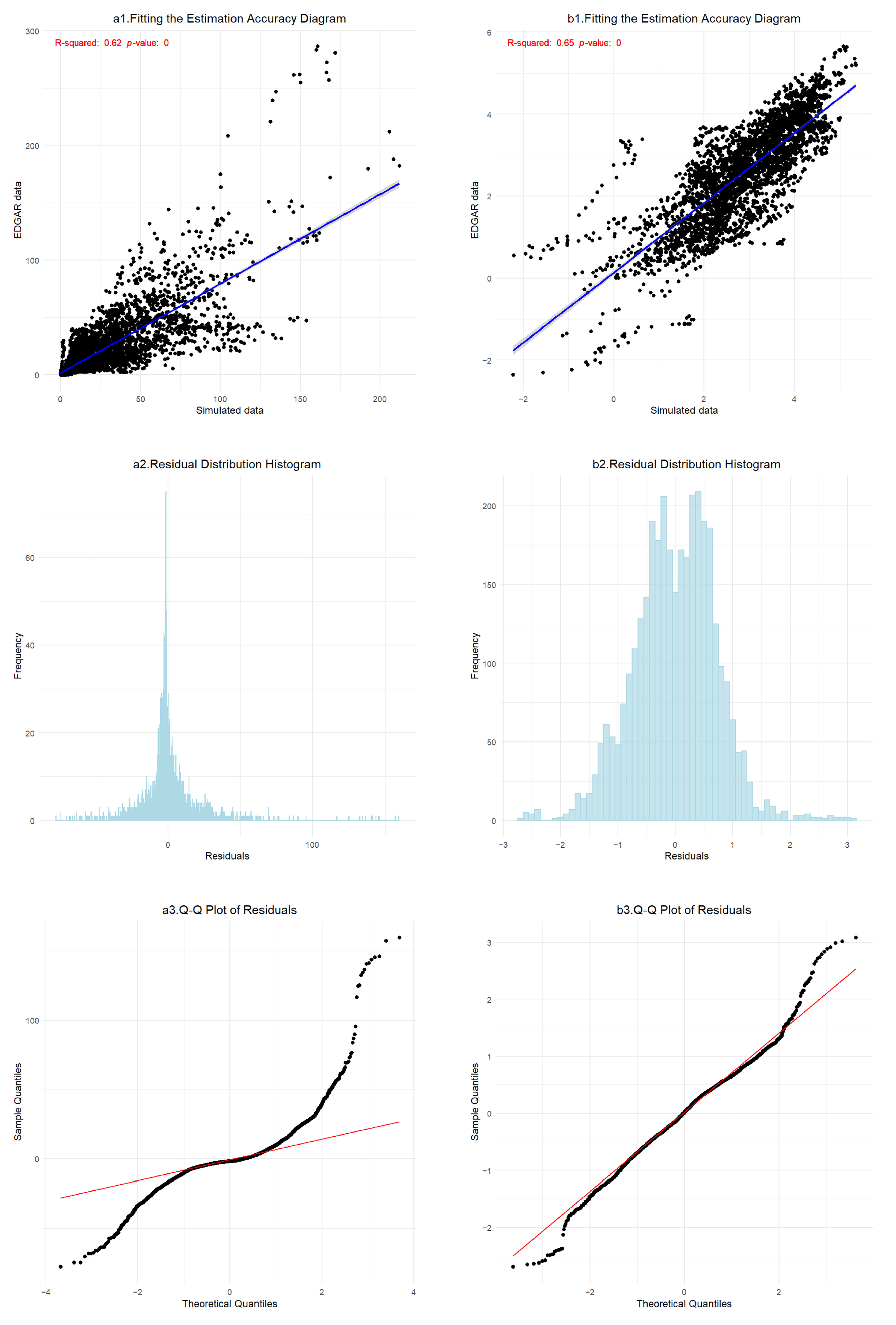
- Crippa, M.; Guizzardi, D.; Pagani, F.; Banja, M.; Muntean, M.; Schaaf, E.; Becker, W.; Monforti Ferrario, F.; Grassi, G.; Rossi, S.; et al. EDGAR v8.0 Greenhouse Gas Emissions; European Commission, Joint Research Centre (JRC): Brussels, Belgium, 2023. [Google Scholar]
- Xia, H.; Zhao, X.; Sha, Y. HSPEI: A 1-km spatial resolution SPEI Dataset across Chinese Mainland from 2001 to 2022. Geosci. Data J. 2024, 11, 479–494. [Google Scholar] [CrossRef]
- Gao, J.; Shi, Y.; Zhang, H.; Chen, X.; Zhang, W.; Shen, W.; Xiao, T.; Zhang, Y. China Regional 250m Fractional Vegetation Cover Data Set (2000–2023); National Tibetan Plateau/Third Pole Environment Data Center: Beijing, China, 2024. [Google Scholar]
- Sun, H.; Liu, W.; Wang, Y.; Yuan, S. Evaluation of Typical Spectral Vegetation Indices for Drought Monitoring in Cropland of the North China Plain. IEEE J. Sel. Top. Appl. Earth Obs. Remote Sens. 2017, 10, 5404–5411. [Google Scholar] [CrossRef]
- Oak Ridge National Laboratory (ORNL): LandScan Global. Available online: https://landscan.ornl.gov/ (accessed on 26 July 2024).
- National Centers for Environmental Information: Global-Summary-of-the-Day. Available online: https://www.ncei.noaa.gov/data/global-summary-of-the-day/archive/ (accessed on 23 June 2024).
- Donat, M.G.; Lowry, A.L.; Alexander, L.V.; O’Gorman, P.A.; Maher, N. More extreme precipitation in the world’s dry and wet regions. Nat. Clim. Change 2016, 6, 508–513. [Google Scholar] [CrossRef]
- Climate Science Special Report. Fourth National Climate Assessment; US Global Change Research Program: Washington, DC, USA, 2017; Volume I.
- IPCC. Climate Change 2021: The Physical Science Basis. Contribution of Working Group I to the Sixth Assessment Report of the Intergovernmental Panel on Climate Change; Cambridge University Press: Cambridge, UK; New York, NY, USA, 2021. [Google Scholar]
- Srikanth, K.S.; Zimmermann, D. An Implementation of Isolation Forest, Version 1.1.3; R Foundation for Statistical Computing: Vienna, Austria, 2021. [Google Scholar]
- Liu, F.T.; Ting, K.M.; Zhou, Z.-H. Isolation-Based Anomaly Detection. ACM Trans. Knowl. Discov. Data 2012, 6, 1–39. [Google Scholar] [CrossRef]
- Hamaker, E.L.; Kuiper, R.M.; Grasman, R.P.P.P. A critique of the cross-lagged panel model. Psychol. Methods 2015, 20, 102–116. [Google Scholar] [CrossRef] [PubMed]
- Mulder, J.D.; Hamaker, E.L. Three Extensions of the Random Intercept Cross-Lagged Panel Model. Struct. Equ. Model. 2021, 28, 638–648. [Google Scholar] [CrossRef]
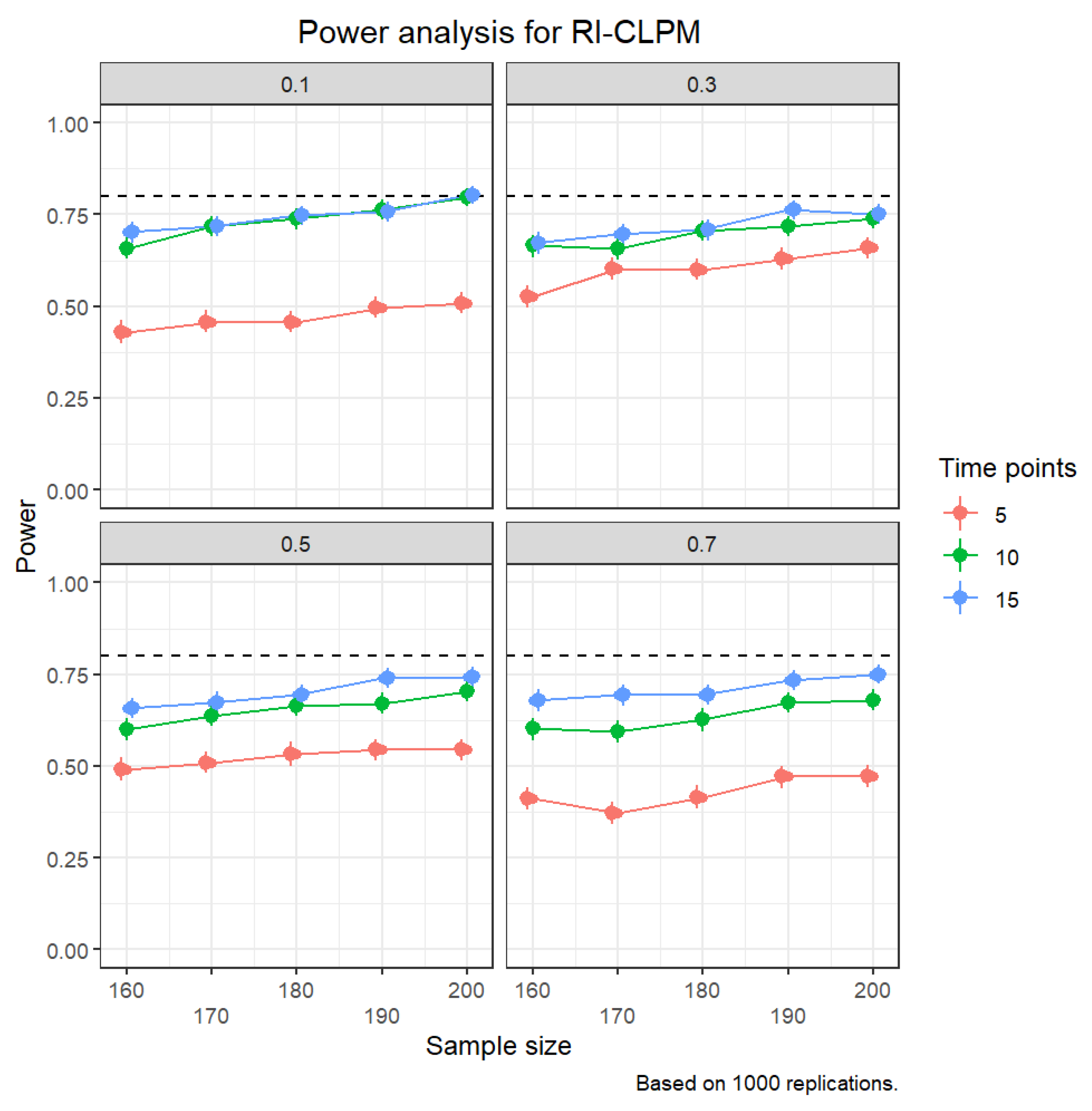
- Mulder, J.D. Power Analysis for the Random Intercept Cross-Lagged Panel Model Using the powRICLPM R-Package. Struct. Equ. Model. 2023, 30, 645–658. [Google Scholar] [CrossRef]
- Chen, J.; Lei, X. Measurement of Interregional Knowledge Spillover in China. Sci. Technol. Prog. Policy 2010, 27, 39–44. [Google Scholar]
- Ye, A.; Wu, J.; Chen, S. Spatial Econometrics; Xiamen University Press: Xiamen, China, 2015. [Google Scholar]
- Elhorst, J.P.; Fréret, S. Evidence of Political Yardstick Competition in France Using a Two-Regime Spatial Durbin Model with Fixed Effects. J. Reg. Sci. 2009, 49, 931–951. [Google Scholar] [CrossRef]
- Elhorst, J.P. Spatial Econometrics; Springer: Berlin/Heidelberg, Germany, 2014. [Google Scholar]
- Elhorst, J.P. Matlab Software for Spatial Panels. Int. Reg. Sci. Rev. 2014, 37, 389–405. [Google Scholar] [CrossRef]
- Rosseel, Y. Lavaan: An R Package for Structural Equation Modeling. J. Stat. Softw. 2012, 48, 1–36. [Google Scholar] [CrossRef]
- Stoel, R.D.; Garre, F.G.; Dolan, C.; van den Wittenboer, G. On the likelihood ratio test in structural equation modeling when parameters are subject to boundary constraints. Psychol. Methods 2006, 11, 439–455. [Google Scholar] [CrossRef]
- Kuiper, R. ChiBarSq. DiffTest: Chi-Bar-Square Difference Test of the RI-CLPM Versus the CLPM and More General[Computer Software Manual], version 0.0.0.9000; R Foundation for Statistical Computing: Vienna, Austria, 2021. [Google Scholar]
- Ji, Y.; Wang, F. Industrial agglomeration, spatial spillover and urban energy efficiency. J. Beijing Inst. Technol. (Soc. Sci. Ed.) 2021, 23, 13–26. [Google Scholar]
- Han, F.; Yang, L. How does the agglomeration of producer services promote the upgrading of manufacturing structure?: An integrated framework of agglomeration economies and schumpeter’s endogenous growth theory. Manag. World 2020, 36, 72–94. [Google Scholar]
- Wei, X.H.; Zhang, C.; Shen, T.Y. Software for Spatial Econometrical Analysis: Operation Manual of R Language; Peking University Press: Beijing, China, 2022. [Google Scholar]
- Wang, K.; Wu, S.; Gao, H.; Wang, C. Research on the Influence of Air Pollution on Green Technology Innovation of Listed Companies in Heavy Pollution Industries. Chin. J. Manag. 2023, 20, 400–410. [Google Scholar]
- Ma, X.; He, J. Air pollution and corporate green innovation in China. Econ. Model. 2023, 124, 106305. [Google Scholar] [CrossRef]

| Variable | Obs | Mean | SD | Min | P25. | Median | P75. | Max |
|---|---|---|---|---|---|---|---|---|
| SPEI | 1640 | 0.103601 | 0.205118 | −0.719655 | −0.014255 | 0.115136 | 0.229059 | 0.736612 |
| ln(Carbon) | 1640 | 3.219701 | 1.023457 | −0.114833 | 2.496734 | 3.369444 | 4.000356 | 5.356 |
| FVC | 1640 | 0.484902 | 0.195377 | 0.039246 | 0.385403 | 0.524377 | 0.609315 | 0.841243 |
| Ext_Wea | 1640 | 0.104471 | 0.034878 | 0.027322 | 0.079235 | 0.101093 | 0.126027 | 0.224658 |
| ln(Pop) | 1640 | 4.827631 | 1.545234 | −0.064976 | 4.12421 | 5.137982 | 6.044447 | 7.133607 |
| Ind_Str | 1640 | 1.244828 | 0.826715 | 0.130402 | 0.712861 | 1.014653 | 1.543616 | 6.068421 |
| lag_ln(Carbon) | 1640 | 3.192188 | 1.031743 | −0.449434 | 2.476308 | 3.328708 | 3.967777 | 5.356 |
| lag_SPEI | 1640 | 0.102429 | 0.197656 | −0.619156 | −0.017313 | 0.108866 | 0.225859 | 0.736612 |
| RGDP | 1640 | 1381.57 | 2213.507 | 23.86415 | 353.4547 | 788.3353 | 1461.394 | 27,564.79 |
| Metric | Value_Standard | Value_Scaled | Type |
|---|---|---|---|
| Chi-square | 744.277 | 519.352 | Fit Index |
| Degree of Freedom | 141 | 141 | |
| p-value (Chi-square) | 0 | 0 | |
| CFI | 0.931 | 0.939 | |
| TLI | 0.906 | 0.918 | |
| RMSEA | 0.158 | 0.125 | |
| 90% CI RMSEA (Lower) | 0.147 | 0.116 | |
| 90% CI RMSEA (Upper) | 0.169 | 0.135 | |
| p-value RMSEA ≤ 0.05 | 0 | 0 | |
| SRMR | 0.112 | 0.112 | |
| AIC | −3434.249 | Information Criterion | |
| BIC | −3154.641 | ||
| SABIC | −3436.453 |
| Year | ln(Carbon) | SPEI |
|---|---|---|
| 2012 | 0.4581 *** | 0.7869 *** |
| 2013 | 0.4296 *** | 0.8468 *** |
| 2014 | 0.4060 *** | 0.7528 *** |
| 2015 | 0.3972 *** | 0.8753 *** |
| 2016 | 0.3940 *** | 0.6811 *** |
| 2017 | 0.4047 *** | 0.7957 *** |
| 2018 | 0.4268 *** | 0.8469 *** |
| 2019 | 0.4370 *** | 0.8566 *** |
| 2020 | 0.4550 *** | 0.7502 *** |
| 2021 | 0.4388 *** | 0.6845 *** |
| Variable | Dynamic | Non-Dynamic |
|---|---|---|
| ρ | 0.8397 *** (90.311) | 0.8468 *** (93.547) |
| ln(Carbon) | −0.0106 (−0.5387) | −0.0106 (−0.5378) |
| FVC | 0.5732 *** (4.3896) | 0.5865 *** (4.4512) |
| Ext_Wea | −0.3876 *** (−4.2606) | −0.3612 *** (−3.9441) |
| ln(Pop) | 0.1867 (1.4866) | 0.1900 (1.5011) |
| Ind_Str | 0.0007 (0.1141) | 0.0040 (0.6419) |
| lag_ln(Carbon) | 0.0026 (0.1485) | 0.0020 (0.1106) |
| lag_SPEI | 0.0744 *** (5.9497) | |
| W.ln(Carbon) | −0.0628 ** (−2.5133) | −0.0581 ** (−2.3095) |
| W.FVC | −0.0260 (−1.0645) | −0.0225 (−0.9179) |
| W.Ext_Wea | 0.0743 (1.1998) | 0.0783 (1.2552) |
| W.ln(Pop) | 0.0044 (1.3705) | 0.0037 (1.1526) |
| W.Ind_Str | 0.0039 (1.1007) | 0.0021 (0.6055) |
| W.lag_ln(Carbon) | 0.0567 ** (2.2963) | 0.0552 ** (2.2191) |
| W.lag_SPEI | 0.0136 (1.1619) | |
| logLik | 1657.625 | 1638.826 |
| R² | 0.8599 | 0.8577 |
| Variable | Dynamic | Non-Dynamic | ||||
|---|---|---|---|---|---|---|
| Direct Effects | Spatial Spillover | Total | Direct Effects | Spatial Spillover | Total | |
| ln(Carbon) | −0.0470 | −0.4082 ** | −0.4552 ** | −0.0460 | −0.3996 ** | −0.4456 ** |
| lag_ln(Carbon) | 0.0326 | 0.3354 ** | 0.3680 * | 0.0319 | 0.3385 * | 0.3704 * |
| Variable | Dynamic | Non-Dynamic | ||||
|---|---|---|---|---|---|---|
| Direct Effects | Spatial Spillover | Total | Direct Effects | Spatial Spillover | Total | |
| ln(Carbon) | −0.0726 ** | −0.5317 *** | −0.6044 *** | −0.0730 ** | −0.5383 *** | −0.6113 *** |
| lag_ln(Carbon) | 0.0319 | 0.3365 * | 0.3684 * | 0.0320 | 0.3456 * | 0.3776 * |
| Variable | Dynamic | Non-Dynamic | |||||
|---|---|---|---|---|---|---|---|
| Direct Effects | Spatial Spillover | Total | Direct Effects | Spatial Spillover | Total | ||
| From 2012 to 2016 | ln(Carbon) | 0.0215 | −0.0419 | −0.0204 | 0.0265 | −0.0136 | 0.0129 |
| lag_ln(Carbon) | −0.0249 | 0.0141 | −0.0107 | −0.0304 | −0.0080 | −0.0384 | |
| From 2017 to 2021 | ln(Carbon) | −0.1541 ** | −1.015 *** | −1.1692 *** | −0.1694 ** | −1.1325 *** | −1.3019 *** |
| lag_ln(Carbon) | 0.0035 | 0.4208 | 0.4242 | 0.0110 | 0.4727 | 0.4838 | |
Disclaimer/Publisher’s Note: The statements, opinions and data contained in all publications are solely those of the individual author(s) and contributor(s) and not of MDPI and/or the editor(s). MDPI and/or the editor(s) disclaim responsibility for any injury to people or property resulting from any ideas, methods, instructions or products referred to in the content. |
© 2025 by the authors. Licensee MDPI, Basel, Switzerland. This article is an open access article distributed under the terms and conditions of the Creative Commons Attribution (CC BY) license (https://creativecommons.org/licenses/by/4.0/).
Share and Cite
Zhai, G.; Chu, T. Assessing Carbon Emissions’ Impact on Drought in China’s Arid Regions: Cross-Lagged and Spatial Models. Sustainability 2025, 17, 1891. https://doi.org/10.3390/su17051891
Zhai G, Chu T. Assessing Carbon Emissions’ Impact on Drought in China’s Arid Regions: Cross-Lagged and Spatial Models. Sustainability. 2025; 17(5):1891. https://doi.org/10.3390/su17051891
Chicago/Turabian StyleZhai, Guangyu, and Tianxu Chu. 2025. "Assessing Carbon Emissions’ Impact on Drought in China’s Arid Regions: Cross-Lagged and Spatial Models" Sustainability 17, no. 5: 1891. https://doi.org/10.3390/su17051891
APA StyleZhai, G., & Chu, T. (2025). Assessing Carbon Emissions’ Impact on Drought in China’s Arid Regions: Cross-Lagged and Spatial Models. Sustainability, 17(5), 1891. https://doi.org/10.3390/su17051891