Abstract
In this paper, controllable wind turbines are employed for emergency frequency control to reduce cost. However, controllable wind turbines introduce significant modeling uncertainties in the form of uncertain environmental factors and model aggregation into the system. To pre-generate feasible emergency control strategies at the lowest cost, a robust optimization model is constructed for a potentially serious fault in power systems, which is a mixed-integer nonlinear robust programming issue with non-analytical calculation (for post-event system frequency). Therefore, this study proposes to first quantify the impact of modeling uncertainties on wind turbine regulation and find the most unfavorable uncertain scenarios for emergency frequency control. Then, based on the above-filtered scenarios, the original problem is transformed into mixed-integer nonlinear programming. A novel simplified algorithm is proposed to solve the above problem efficiently. Finally, a case study is conducted on a real regional power system. It is proved effective in reducing costs by regulating wind turbines for emergency control, and the proposed method is effective in dealing with the impact of modeling uncertainties. Also, high solving efficiency (12 s in case study) meets the demand for efficient online pre-decision-making for emergency control. The research is meaningful in the promotion of secure access to power systems for sustainable power.
1. Introduction
Increases in power electronic interface sources in power systems worsen the dynamic characteristics of system frequency due to reduced system inertia [1,2]. In addition, in well-developed large-scale regional interconnected power systems, the risk and severity of frequency instability may increase due to possible faults of transmission lines [3]. Therefore, to solve these problems, it is imperative to develop innovative emergency frequency control (EFC) strategies.
For EFC, load shedding and generator tripping are considered feasible solutions [4,5]. Although these measures provide the fastest frequency support, they still have drawbacks, such as high costs and discrete control modes. The urgent need for active power support decreases over time following emergency faults that worsen system frequency. Examples of active power support include the inertial response process and primary frequency control [6], as the name of the inertial response period suggests, system inertia plays a dominant role in suppressing rapid changes in system frequency, as conventional generators (CGs) provide extremely restricted power support in the initial post-fault period. Equipment-tripping measures yield tremendous benefits during this process. Additionally, partially replacing these costly procedures with more cost-effective ones is promising for rapid frequency support during the initial response period. For example, wind turbines (WTs) can be regulated rapidly for power support using rotor kinetic control [7,8]. Specifically, a WT can release or store kinetic energy in its rotor through temporary changes in rotor speed, and its normal operation remains unaffected. Unfortunately, WT operation exhibits relatively high uncertainties, due to time-varying environmental conditions [9]. Accordingly, some random distribution models have been constructed to address these uncertainties of wind speed and wind power. These models assume a specific distribution structure or rely on extensive historical data analysis [10,11]. In addition to volatile environmental factors, the modeling errors of the WT control structure are also not negligible, as they are introduced through the monitoring data, aggregation area, and identification algorithm used [12]. Furthermore, the control master can be duped into creating improper control orders since these uncertainties will be included in the post-event system frequency computation.
Naturally, to sustain the power system’s post-event security operation (regarding system frequency and WT operation) at the lowest control cost, the EFC strategy, which is significantly complex, must be robustly optimized. Firstly, based on the system frequency response (SFR) model, non-analytical numerical integration is typically required to calculate the dynamic response (the nadir and steady-state value) of the system frequency, especially while considering various nonlinear factors, such as dead band and amplitude limitation [13,14]. Secondly, the problem exhibits mixed-integer characteristics. Lastly, but significantly, the modeling uncertainties of WTs are coupled with the aforementioned complex characteristics, and the whole problem is presented as a robust mixed-integer nonlinear programming (MINLP) issue with non-analytical calculation. Typically, the control master is required to solve the optimization problem periodically, to pre-generate decisions for a potentially serious fault (such as the blocking fault of the DC transmission system in the sending-end grid) [15]. Therefore, rapid model solving is required to refresh pre-decision results, ensuring the efficiency of the “offline computation and online matching” mode.
Some well-established theories have been put forth specifically for linear robust optimization issues [16]. Nonlinear robust optimization theory usually requires certain application scenarios. For example, some stochastic optimization methods have to model the distribution of uncertain parameters in advance, which may pose practical challenges for real power systems [17,18]. Also, most of these methods lean towards employing a fully analytical model as a solving foundation, which does not apply to the above problem in this paper [19,20]. Thus, addressing the above robust problem directly is challenging. Moreover, for EFC with controllable WTs, it is proposed to decouple the modeling uncertainties of the WTs from the security constraints first. Then, the original robust problem is approximated without uncertain factors and is further simplified into a mixed-integer linear programming (MILP) problem. Specifically, the contributions of this work are as follows:
- Firstly, this work proposes to quantify the impact of modeling uncertainties on WT regulation through trajectory sensitivity to find the worst cases for frequency support. Then, the original robust problem can be decoupled from the modeling uncertainties.
- For the reformulated problem without uncertainties, which retains complex characteristics, a novel systematic mixed-integer linearization method is proposed.
The rest of this paper is organized as follows: The whole robust optimization model for EFC is presented in Section 2. In Section 3, the robust problem is transformed into an optimization problem without uncertainties, using the proposed method for quantifying the impact of modeling uncertainties on WTs. Then, a systematic mixed-integer linearization method for solving the above optimization problem is introduced in Section 4. A case study is presented in Section 5, and the conclusion is summarized in Section 6.
2. Optimization Model of Emergency Frequency Control Strategy
2.1. SFR Model Coupled with Uncertain Parameters
An SFR model involving the mathematical models of WTs and CGs is necessary for modeling the post-event system frequency. Thus, in considering the time scale of the frequency control while ignoring electromagnetic transient dynamics, a simplified model of the active power regulation of a WT is shown in Figure 1 [21]. Here, a doubly fed induction generator is shown as an example.
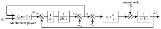
Figure 1.
Simplified model of active power control system of the wind turbine.
In the figure, ΔPw denotes the change in the output power of the WT; ω0, Δω, and ω denote the initial, deviation, and real-time values of the rotor speed, respectively; β0 is the initial pitch angle; ωref denotes the reference value of the rotor speed, and ω0 is often set to ωref, due to the maximum power point tracking operation; ωn is the rated rotor speed; Hw represents the inertia constant of the multiple masses of the WT; and kp and ki are control parameters. The Pulse-Width Modulation (PWM) segment is simplified as the inertial element with time constant Tw. The variation in mechanical power ΔPwm is calculated based on the aerodynamic equations of the blade, denoted as fpm. While assigning a negative order Pf to the WT, the dynamic response of its output power and rotor speed can be approximated, as illustrated in Figure 2.
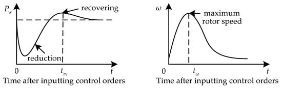
Figure 2.
Dynamic response of the WT after giving the order Pf.
In this figure, trv and tω record the time point when the output reaches the maximum value during its recovery (to the initial value) and when the rotor speed reaches its nadir, respectively.
Here, possible parameter values of the ith WTs are uniformly designated as ψi within the error boundary, as follows:
where is the number of uncertain parameters; pdown,k and pup,k denote the lower and upper limits, respectively. Specifically, in the active regulation model of the wind turbine, this paper focuses on its five uncertain parameters, including the initial rotor speed ω0, the inertia constant of the multiple mass of the WT Hw, the initial pitch angle β0, and the control parameters kp and ki. These uncertainties of the above parameters are mainly introduced by variations in the environment and operating conditions, as well as by errors in the aggregation modeling of the WT.
To simplify the expression, set function G(·) to represent the relationship model in Figure 1, with Pf as the input and ΔPw as the output. Then, the detailed SFR model for EFC is presented in Figure 3.
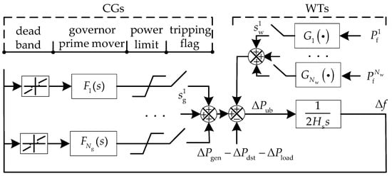
Figure 3.
The detailed SFR model for EFC considering WTs and CGs.
Here, the controls of the generators (ΔPgen) and loads (ΔPload) are both involved in this model, though only one of them will be adopted when faced with a specific fault (ΔPdst). Ng and Nw denote the number of CGs and WTs, and
is a binary variable, with ‘0’ indicating that the ith CG is tripped. Similarly, corresponds to the jth WT, Fi(s) denotes the transfer function model of the governor and prime mover of the ith CG, and Gj(·) is the aforementioned simplified expression of the jth WT. Hs is the system inertia, and the system frequency deviation Δf is motivated by the real-time unbalanced power ΔPub. However, due to Gj(·) (j = 1~Nw) involving possible parameter errors in Equation (1), the system frequency calculation is indeed coupled with uncertainties.
2.2. Constructing the Optimation Model for Robust EFC
The main distinction between EFC handling the fault contributing to a rising frequency and dropping frequency lies in whether the equipment removed is the load or the generator. If solely considering the solving process of the EFC optimization problem, the variation may be minimal. Therefore, for simplicity, in the subsequent sections, only one of them (the fault-inducing rising frequency) is considered for illustration and analysis purposes. Specifically, the security of the system frequency, rotor speed of the WTs, and post-event power flow of the transmission lines are considered, and a robust optimization model aiming to minimize costs for EFC is established. Specifically, the decision variables include (i = 1~Ng, a binary variable denoting the tripping signal of the ith CG), (j = 1~Nw, a binary variable denoting the tripping signal of the jth WT), and (k = 1~Nw, a real variable denoting the control order of the kth WT). The objective is to minimize the control cost, considering the cost of tripping generators and regulating WTs, as shown in Equation (2). Control costs are traditionally calculated in the form of unit control costs multiplied by control quantities [4,22]. The security constraints are expressed as Equation (3).
where these constraints are organized in a general form. For example, the transient frequency nadir fmax (with its security limit ) and the rotor speed peak of the kth WT (with the security limit ) are usually calculated via numerical integration based on the model in Figure 2 and Figure 3, respectively [23]. That is, they are related to the uncertain parameters ψ of the WTs. , , and denote the cost coefficients for tripping the ith CG, tripping the jth WT, and regulating the kth WT; and describe the initial power of the CG and the WT; fres denotes steady-state frequency, with f as its upper security limits; and Ωln describes the set of transmission lines. Pm–n is the active power flow of transmission line m–n, with security limit . Here, the method of DC power flow is applied to simplify the calculation [24].
Regarding the problem of Equations (2) and (3), there are two main issues for an efficient solution: (1) the coupling of the system frequency calculation and modeling uncertainties; (2) the coupling of the mixed-integer, nonlinear, and non-analytical characteristics. The two issues will be analyzed and addressed in Section 3 and Section 4, respectively.
3. Decoupling the Optimization Constraints and Modeling Uncertainties
3.1. Model Construction for Estimating the Worst Impact of Uncertain Parameters on Optimization Constraints
From the perspectives of both the security of WTs and the power system, the possible deviation in uncertain WT parameters may lead to the following two worrisome scenarios for EFC strategy formulation:
- (1)
- With the known modeling results of uncertain parameters ψ0, the rotor speed peak of the WT under control order Pf is calculated to be lower than its real value, which will make us provide overly aggressive control orders during decision-making. This may compromise the security of the actual rotor speed.
- (2)
- With the given parameters ψ0, the simulated curve about the transient power output of the WT is ‘superior’ to its actual value in terms of frequency support, which will lead us to provide undersized control orders, resulting in insufficient actual power regulation, and threatening system frequency security.
Here, the worst possible situations in terms of the above two scenarios are denoted as Sω and Sf, respectively, with the corresponding actual parameters ψω and ψf. If the optimal control orders are provided such that they fully satisfy the security constraints under both Sω and Sf, they will always be robust regardless of any other possible parameter combination. Here, for ease of description, the following analysis mainly focuses on a single WT, and some superscripts (such as i in ) denoting WT indices are omitted temporarily. In the first scenario Sω, the maximum possible value of the rotor speed peak under a fixed order Pf can be provided by solving an optimization problem as follows:
where fwmax illustrates the relationship of ωmax being influenced by ψ and Pf in Figure 1.
In the second scenario Sf, an ‘inferior’ output curve is expected, which refers to the slightest contribution preventing the system frequency from rising. As mentioned earlier, the participation of wind power regulation is most pronounced in the initial post-event period and gradually decreases with the proportion of power regulation from the CGs increasing over time. Therefore, an index ΔEw evaluating the WT’s ability to support system frequency is defined in this paper, and this index is the weighted integral of the power regulation of the WT over time. In Equation (5), the integration process is expressed as a summation over discrete time points:
where ΔPw is a vector consisting of time series data of power variation ΔPw. Here, the integration duration tdy is required to be slightly larger than trv (Figure 2) so that the negative impact of the reverse power regulation can also be considered. In taking tsp as a discrete step, Ndy is the total number of time points. The weight coefficient vector α is set to α(k) = (Ndy − k)/Ndy, a known variable. Therefore, the optimization problem for scenario Sω is constructed as follows:
where function few denotes the impact of ψ and Pf.
3.2. Model Simplification and Solution Based on Trajectory Sensitivity Calculation
To solve Equations (4) and (6), it is necessary to calculate the dynamic response of ΔPw and ω based on the state space equations transformed by the WT model in Figure 1 as follows [24]:
where x and denote the state vector and its derivative concerning time, including Δω and ; y denotes the algebraic vector, where ΔPw is its element; u denotes the input vector, including Pf; and f(·) and g(·) are the state equations and algebraic equations.
While the actual value of ψ is exactly equal to the given values ψ0, the dynamic response of ω and ΔPw is calculated and recorded as (vector including ω at every time point) and . The rotor speed peak and its occurrence time (tω in Figure 2) are also recorded here. Then, it is proposed to quantify the impact of possible parameter variation by calculating the trajectory sensitivity, instead of repeated numerical integration, to figure out the dynamic response of the WT under arbitrary parameter combinations. Trajectory sensitivity denotes the change in the dynamic response track at every time point caused by unit variation in model parameters, which can be calculated by taking a partial derivative of Equation (7) concerning parameters ψ, as follows [25]:
where fψ(·) and gψ(·) denote the partial derivative of fψ(·) and gψ(·) about ψ, and xψ denotes the trajectory sensitivity of x about parameters ψ, in which the relationship of ω and ψ is quantified. Also, yψ corresponds to y. Based on the recorded results under ψ0, xψ, and yψ can be further given by Equation (8). In particular, the trajectory sensitivity of ΔPw and ω about ψ are described as [Pw|ψ] and [ω|ψ] and represented as matrixes with Ndy (total time points) rows and Nψ columns (total uncertain parameters). Therefore, based on and [ω|ψ], the curve of the actual rotor speed ωis approximated as follows:
where k denotes the kth time point, and the operator (k,:) denotes selecting the elements of the kth row of the matrix. If time moment tω (the Nωth time point) is selected, the actual rotor speed peak can be approximated, the problem (4) is further transformed into a linear programming problem as follows:
where [ω|ψ] is known, calculated by Equation (8) in advance. Similarly, problem (6) is also simplified as a linear problem as follows:
Finally, when providing a control order Pf, the worst power-regulating curve ΔPw.wst for frequency support and the maximum possible rotor speed peak ωmax.wst are naturally obtained.
3.3. Eliminating Uncertain Model Parameters in the Original Robust Optimization Problem
However, it is impractical to obtain ωmax.wst and ΔPw.wst under every feasible control order by solving Equations (10) and (11). To address this, piecewise linearization is adopted. Firstly, the range of Pf (from −1 p.u. to 0) is divided into several intervals, with Np piecewise interval endpoints Pf,1… Pf, Np. Secondly, problem (10) and problem (11) are solved at these endpoints, with the following results: ωmax.wst,i and ΔPw.wst,i corresponding to Pf,i (i = 1…Np). Finally, for arbitrary order Pf, the corresponding ωmax.wst and ΔPw.wst are described as follows:
where, zpc,i (i = 1~Np − 1) and upc,j (j = 1~Np) are the introduced binary and real variables.
Further, when comparing ωmax.wst (under different Pf) with the security limits ωlm, the maximum (in absolute value) feasible control order Pf.lm is determined, which can fully maintain the operating security of the WT against any uncertain factor. For the security of the post-event system frequency, the linear model of Equations (12) and (13) with Pf as the input and ΔPw.wst as the output is substituted into the SFR model instead of the output order response function G(·) in Figure 3, as shown in Figure 4. As mentioned above, ΔPw.wst,i (i = 1~Np) and Pf.lm are known in advance. Therefore, in taking the decision variables of the WT (Pf and sw) as the input, the model in Figure 4 can output the maximum possible frequency nadir fmax.wst. Further, the original constraints are reorganized in Equation (15).
where the Pf limitation replaces the original constraints on rotor speed. The first-row constraints represent the mathematical expression of Figure 4. However, the formulation is still related to the nonlinear SFR model in Figure 3. Therefore, Section 4 addresses the issue of accelerating model solving.
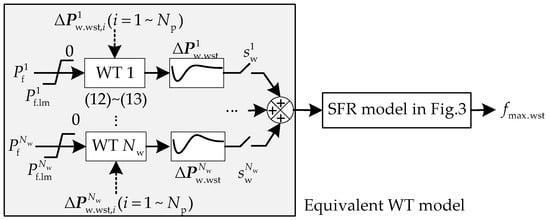
Figure 4.
The simplified regulating-response structure of WT incorporated into the SFR model.
4. Model Simplification by Eliminating Non-Analytical and Nonlinear Calculation
4.1. Differential Discrete Process for the Linear Structure
Fundamentally, the SFR model in Figure 3 for frequency simulation combines a linear structure (transfer function), nonlinear segments (such as the dead band), and integer variables. For example, the structure of the CGs in Figure 3 is exactly typical.
In the Figure 5, denotes frequency deviation over the dead band, and Δ and Δ denote the power regulation reference before and after the power limit segment, where the actual power regulation Δ will be set to 0 if the ith CG is tripped (= 0).
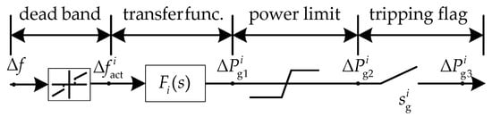
Figure 5.
Structure of primary frequency regulation of the ith CG.
The transfer functions are the main source of the non-analytical computation. Here, motivated by the optimization principle of the traditional model’s predictive control process, in which some intermediate variables at different time points are augmented as decision variables to accelerate model solving [26], a novel model simplification method is proposed in this paper, involving discrete model differences and decision variable augmentation for the inherently linear transfer function.
Specifically, as an example, Fi(s) in Figure 5 can be discretized into a z-domain transfer function through a bilinear transformation, and the time domain difference equations concerning the input Δf and the output Δ can then be further developed as follows [24]:
where denotes the kth time point, Ndy denotes the total time points, l denotes the order of the transfer function, and αm and βn are constant coefficients. Note that there are a total of Ndy linear equations in Equation (16) just for this one transfer function.
Then, at every time section, these variables (Δ(k), Δ(k), k = 1…Ndy) in Equation (16) are supplemented as new decision variables. The linear equations in Equation (16) are also supplemented as new constraints corresponding to the system frequency requirement of the optimization model of Equations (2) and (15). Of course, for every transfer function in Figure 3, the corresponding variables and equations are all processed in the same way. So far, the iteration calculation is eliminated by describing the mathematical constraints of variables at different time points.
4.2. Mixed-Integer Linearization for Nonlinear Components
There are two main types of nonlinear components in the SFR model in Figure 3. Firstly, the Big M method is adopted to deal with the segment about logical judgment (such as the dead band, the power limit, and the judgment regarding tripping CGs) [27]. Due to space constraints, a detailed explanation will not be provided here. Secondly, the system inertia Hs is the denominator of the transfer function (the equivalent rotor equation) in Figure 3, which is determined using unit combinations as follows:
where Δfr denotes the rate of change in frequency, Si and Hi denote the rated capacity and inertia constant of the ith CG, and SB denotes the reference capacity. Thus, the overall presentation of Equation (17) exhibits nonlinearity. Here, it is proposed to reorganize Equation (17) as follows:
where denotes pre-event (known) system inertia. On the one hand, tripping CGs can cut down the unbalanced power directly. On the other hand, system inertia is reduced, which is equivalent to actually increasing the unbalanced power for motivating frequency fluctuation. Here, this part of unbalanced power is described as Δ. Based on Equation (18), the structure can be reorganized as shown in Figure 6.
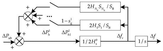
Figure 6.
The reorganized equivalent model about rotor motion equation.
Here, Δ corresponds to Δ, while the ith CG is tripped. The proposed differential discrete process and the Big M method can also be applied to the model. Finally, the original optimization is simplified as a MILP problem, which can be solved efficiently.
4.3. Implementation Process for the Proposed Method
Step 1: The SFR model in Figure 3 is established based on the actual power system for calculating the post-event system frequency. Based on this, the robust optimization models in Equations (2) and (3) are constructed while considering the EFC.
Step 2: The optimization problems of Equations (4) and (5) (simplified as Equations (10) and (11)) are constructed to search for the uncertain scenarios Sω and Sf that are most unfavorable for wind turbines implementing EFC. Just for scenarios Sω and Sf, the robust issues of Equations (2) and (3) constructed in Step 1 are transformed into the MINLP issue of Equations (2) and (15).
Step 3: The complex optimization problems Equations (2) and (15) obtained in Step 2 are transformed into a MILP through the process of Equations (16)–(18).
Step 4: The MILP problem in Step 3 is solved using the CPLEX 12.8 software, and the optimal control orders (sg, sw, and Pk) are provided.
5. Case Study
5.1. System Description
The simulation was based on a regional DC sending-end power grid, and its simplified topology is illustrated in Figure 7. The grid mainly includes three voltage levels: 110 kV, 220 kV (the thin black lines in Figure 7), and 500 kV (the thick black lines). Here, 110 kV buses are not depicted due to space limits. There were 19 CGs with 18.3 million kW, including 5 hydro generators and 14 thermal generators, as shown by the blue marks in Figure 7. In addition, 20 controllable wind turbines (representing wind farms) were distributed as shown by the green marks in Figure 7 with 7.09 million kW. Here, some generators (WTs or CGs) share common grid-connected points. There is a DC transmission system at bus 10, with a bipolar sending capacity of 6 million kW. Here, some operational data of the power grid were extracted during a certain period as the foundation for subsequent simulations. Some parameters about the system are provided in Appendix A.
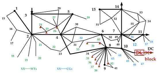
Figure 7.
The simplified topology of the regional DC sending-end power grid for simulation.
The error range of the WT parameters (ω0, β0, Hw, kp, and ki) in Equation (1) was regarded as ±5%, and were 50.2 Hz and 50.5 Hz [28], and tdy and tsp (for optimization) were 15 s and 0.02 s, respectively. The following plots show the dynamic simulations over a longer period for a clearer description. Here, the unit cost coefficients C1, C2, and C3 were set to 3000, 550, and 150 USD/ten thousand kW. Based on this, the EFC strategy for the bipolar blocking of the DC transmission system at bus 10 was formulated considering the power regulation of the WTs.
All simulations are run on a desktop computer with an Intel Dual Core i7-8700 3.2 GHz CPU and 16,384 MB RAM using the MATLAB 2016b platform. It is worth stating that the constructed simulation model is the SFR model (similar to Figure 1) based on Simulink, not a detailed large grid model. The SFR model is constructed by some linear transfer functions (such as the primary frequency control of CGs) and nonlinear state space equations (such as the control structure of WTs). Compared to a detailed large grid model, the SFR model can calculate the post-event system frequency dynamics more efficiently, and some studies have shown that proper high-order nonlinear SFR models have high accuracy in system frequency calculation [13].
5.2. The Two Worst Scenarios of Controllable WTs
Based on the piecewise linearization, control order Pf is divided into different segments with the interval endpoints including −1, −0.75, −0.5, and −0.25 p.u. Here, taking W1 (the WT numbered ‘1’) under control order Pf = −1 p.u. as an example, the regulating response dynamics of W1 with parameters ψ0 (ω0 = 1.02 p.u., β0 = 0°, Hw = 3.5 s, kp = 2 and ki = 0.3) were simulated. As a comparison, an extra three sets of model parameters generated randomly within the error range were applied, and the dynamic response is described as shown in Figure 8. Subsequently, the trajectory sensitivity of these uncertain parameters was calculated, as shown in Figure 9 and Figure 10.
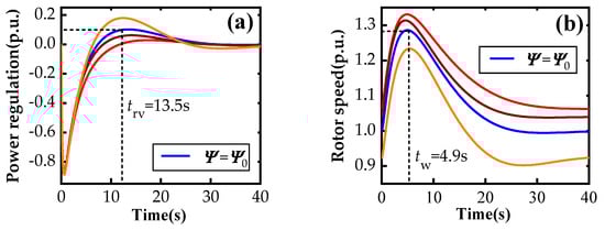
Figure 8.
The dynamic response of the W1 with various uncertain parameters: (a) power regulation. (b) rotor speed. (The blue line corresponds to the results under normal parameters, and the other three lines correspond to the other three sets of parameters).
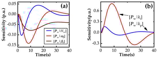
Figure 9.
Trajectory sensitivity of output power about uncertain parameters: (a) Hw, ω0, and β0; (b) ki and kp.
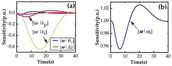
Figure 10.
Trajectory sensitivity of rotor speed about uncertain parameters: (a) Hw, ki, kp, and β0; (b) ω0.
Where, ‘p.u.’ denotes the per unit, which is relative to the baseline value. The real value of a variable is equal to the product of its per unit value and its baseline value. The baseline value of power regulation in Figure 8a is the capacity of the wind turbine W1, and the baseline value of the rotor speed in Figure 8b is the nominal rotor speed of the wind turbine W1.
It can be seen that different parameters contribute to various impacts, and the impacts of the same parameter vary across different periods. Based on the tω selected in Figure 8b, the sensitivities of the rotor speed peak for parameters ψ are extracted from Figure 10. Then, the two worst scenarios (Sω and Sf) are given with corresponding actual parameters (ψω and ψf), as shown in Figure 11. There are significant differences between ψf and ψω due to the different impacts of the same parameter (such as kp) on the output power and rotor speed of the WT, as shown in Figure 9 and Figure 10.
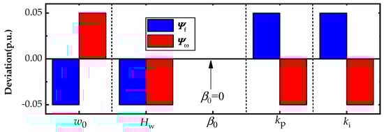
Figure 11.
Model parameters ψf and ψω corresponding to the scenarios Sω and Sf by solving problem (10) and problem (11).
Also, the dynamic response of the power regulation in scenario Sω and rotor speed in scenario Sf was compared with that under model parameters ψ0, as shown in Figure 12. Specifically, the actual deviation in the rotor speed peak under parameters ψω and ψ0 was 0.0590 p.u., as seen in Figure 12b. Here, to verify the accuracy of the trajectory sensitivity calculation, the above deviation can also be approximated using Equation (9) based on the sensitivity results selected at tω = 4.9 s in the curve of Figure 10. The approximated value is 0.0593 p.u., which is sufficiently valid compared to its actual value.
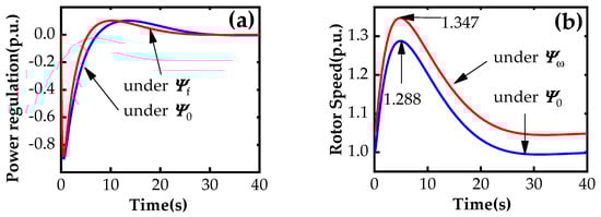
Figure 12.
The dynamic response of W1 under the scenarios Sω and Sf: (a) power regulation under Sf, (b) rotor speed under Sω.
Based on the process outlined in Section 3.3, the maximum feasible control order Pf.lm and the worst regulating response curves ΔPw.wst,i under the control orders (−0.75, −0.5, and −0.25 p.u.) of every WT are provided as the foundation for the subsequent optimization.
5.3. The Robust Emergency Frequency Control Strategy
Regarding the bipolar block fault of the above DC transmission system at bus 10 in Figure 7, the emergency frequency control strategies are optimized under the following three cases:
- Case I: WTs are only allowed to be tripped;
- Case II: WTs can be tripped or regulated without considering their modeling uncertainties;
- Case III: Unlike in Case II, the uncertainties are considered during strategy formulation.
As a result, the optimal strategies under the above three cases are given in Table 1. Note that there is no CG tripped in the three cases due to the number of WTs that can be tripped or regulated. Specifically, in Case I, 15 WTs are tripped with 470.49 ten thousand kW. Only the primary frequency regulation of CGs is employed for the supporting frequency, without regulating WTs. The power response of several CGs (the hydro and thermal generators) is described in Figure 13a, in which G1 is the CG numbered ‘1’. As a result, the frequency peak is around 59.494 Hz, with a steady-state value of 50.116 Hz, as shown in Figure 13b.

Table 1.
The optimal control orders in three cases.
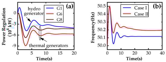
Figure 13.
Control performance of Case I: (a) the dynamic response of CGs, (b) the system frequency.
In Case II, 10 WTs are tripped, and 4 controllable WTs are regulated, as shown in Table 2. Compared to Case I, the steady-state value (50.197 Hz) of the post-event system frequency is close to the security limit (50.2 Hz), which is higher than 50.116 Hz in Case I, as shown in Figure 13b. In contrast, the values of the maximum frequency in both cases are close to the security limit of 50.5 Hz. That is, to ensure the security of the maximum system frequency, more WTs are required to trip in Case I, which contributes to a lower steady-state frequency. However, this seems unnecessary in Case II, as more cost-effective measures (such as regulating WTs rapidly) are adopted to prevent a high peak frequency. The dynamic response of some regulated WTs is displayed in Figure 14.
Table 2.
WTs regulated in Case II and Case III.
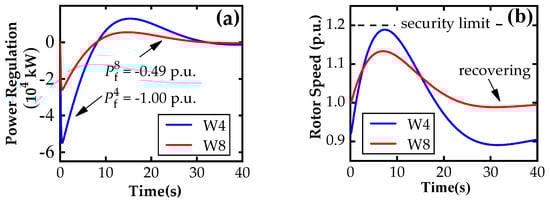
Figure 14.
Dynamic response of WTs in Case II: (a) power regulation (b) rotor speed.
Considering the security constraints of the post-event power flow, the WTs tripped (indicated as ‘▲’ in Figure 7) are mainly located close to the DC transmission system naturally, such as buses 8, 9, and 10, to prevent large-scale power flow transfers. Specifically, around 305.9 ten thousand kW worth of WTs are tripped in the area near buses 8 and 9, while only 74.2 ten thousand kW worth of WTs near buses 2 and 3 (far from bus 10) are tripped. Correspondingly, several lines of 500 kV are displayed in Figure 15. The power flow near bus 10 (such as the line from bus 8 to 9) has undergone significant changes but remains within the security range. For example, the post-event power flow of the line from bus 10 to 7 has increased but is still below its security limit of 450 ten thousand kW.
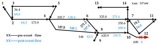
Figure 15.
Pre- and post-event power flow in Case II.
In Case III, the WTs tripped are the same as those in Case II, but more WTs are involved in the regulation to cover the impact of the modeling uncertainties, as shown in Table 2. To verify the robustness of the above-obtained control orders, 100 sets of tests were conducted, in which the model parameters in Equation (1) were randomly generated. Based on the robust control orders in Table 2, the post-event maximum frequency and rotor speed peak of the wind turbines were monitored, as partially displayed in Figure 16.
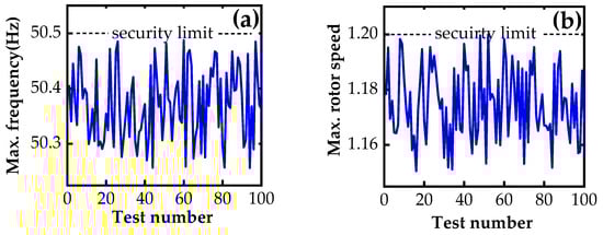
Figure 16.
Post-event performance under robust control in 100 tests: (a) maximum frequency, (b) rotor speed peak of W4.
Obviously, with the robust orders, the maximum frequency in all the tests is below the security limit of 50.5 Hz, and the rotor speed is also within the security range. In comparison, in some scenarios with certain parameter combinations, adopting the non-robust control in Table 2 may contribute to a system frequency beyond the security boundary. For example, for the four WTs (W4, W8, W13, and W19) regulated in Case II with the actual model parameters ψf, their dynamic frequency is described in Figure 17a. While the actual model parameters were ψω, the rotor speed of W4 under the non-robust order exceeded its maximum limit, as shown in Figure 17b. However, the robust control yields satisfactory results, with only a slight increase in WT regulation as a trade-off, as shown in Table 1.
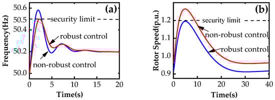
Figure 17.
The post-event performance of robust and non-robust control in some scenarios: (a) system frequency; (b) rotor speed of W4.
Thus, the optimization benefits from the complete set methods for model simplification proposed in Section 4, and multiple repeated tests proved that the optimization can be solved within 12 s for the EFC of the large regional grid, thereby fully meeting the requirements for online applications.
6. Conclusions
An optimization model for an emergency frequency control strategy is constructed by considering the supplemental measures used to regulate wind turbines, which involve a robust mixed-integer nonlinear optimization problem with non-analytical calculation. Therefore, a novel method is proposed to first decouple security constraints with uncertainties, and a set of mixed-integer linearization methods is further proposed to simplify and solve the transformed problem. Based on a case study, the following conclusions are drawn:
- (1)
- The proposed method has the potential to apply some controllable resources, such as wind turbines, to EFC for cost reduction.
- (2)
- Decoupling optimization constraints and modeling uncertainties by estimating the worst scenarios about WT regulation is a valid approach for reducing the complexity of robust optimization while ensuring control robustness.
- (3)
- Adopting the proposed simplification method is an efficient manner of accelerating the nonlinear and non-analytical optimization for EFC, with a time consumption within 12 s for a large regional power grid.
Of course, the SFR model is adopted to calculate the post-event frequency, and some linearization measures are employed to reduce the complexity of the optimization problem, so there may be errors in the calculation results. In addition, modeling uncertainties from the grid side are not considered in the current study, which may also have an impact on the performance of emergency frequency control. Therefore, further research will be conducted on the above two issues to achieve more effective control performance.
Author Contributions
Conceptualization, D.K.; Methodology, G.X. and S.F.; Software, H.Y.; Data curation, H.Y.; Writing—original draft, S.F.; Writing—review & editing, G.X.; Supervision, D.K., S.L. and J.X.; Funding acquisition, G.X. All authors have read and agreed to the published version of the manuscript.
Funding
This work was supported by the major technology project of China Southern Power Grid, “Research on the coupling mechanism and control method of large disturbance stabilization of modern power system” (Project No. 0000002022030101XT00031).
Institutional Review Board Statement
Not applicable.
Informed Consent Statement
Not applicable.
Data Availability Statement
The original contributions presented in this study are included in the article. Further inquiries can be directed to the corresponding author.
Conflicts of Interest
Authors Guanghu Xu and Huanhuan Yang were employed by the company China Southern Power Grid. The remaining authors declare that the research was conducted in the absence of any commercial or financial relationships that could be construed as a potential conflict of interest.
Appendix A
Some parameters of the simulation model are shown as follows:
Table A1.
Parameters of 19 (5 hydro generators and 14 thermal generators) CGs.
Table A1.
Parameters of 19 (5 hydro generators and 14 thermal generators) CGs.
| CG | Pg0 (104 kW) | Hi (s) | CG | Pg0 (104 kW) | Hi (s) |
|---|---|---|---|---|---|
| G1 | 60.24 | 3.00 | G11 | 100.22 | 5.05 |
| G2 | 68.02 | 3.03 | G12 | 120.24 | 3.67 |
| G3 | 68.66 | 3.58 | G13 | 100.46 | 3.36 |
| G4 | 140.22 | 3.86 | G14 | 80.06 | 3.55 |
| G5 | 140.42 | 3.60 | G15 | 80.08 | 3.77 |
| G6 | 80.24 | 3.48 | G16 | 100.06 | 3.7 |
| G7 | 80.40 | 3.64 | G17 | 117.80 | 3.39 |
| G8 | 60.04 | 3.43 | G18 | 120.4 | 3 |
| G9 | 40.02 | 5.00 | G19 | 136.42 | 3 |
| G10 | 140.86 | 5.00 |
Table A2.
(a). Parameters of 20 WTs (W1–W12). (b). Parameters of 20 WTs (W13–W20).
Table A2.
(a). Parameters of 20 WTs (W1–W12). (b). Parameters of 20 WTs (W13–W20).
| (a) | ||||||
| WT | Pw0 (104 kW) | Hw (s) | ω0 (p.u.) | kp | ki | β0 (deg) |
| W1 | 33.05 | 3.50 | 1.02 | 2.00 | 0.30 | 0.00 |
| W2 | 40.52 | 5.03 | 0.97 | 1.91 | 0.28 | 1.12 |
| W3 | 44.80 | 4.58 | 1.00 | 2.06 | 0.29 | 0.38 |
| W4 | 58.00 | 5.86 | 0.91 | 2.03 | 0.30 | 1.02 |
| W5 | 31.05 | 3.6 | 0.96 | 1.97 | 0.27 | 0.75 |
| W6 | 40.15 | 3.48 | 0.96 | 2.04 | 0.28 | 1.34 |
| W7 | 40.00 | 9.28 | 1.02 | 1.93 | 0.32 | 1.46 |
| W8 | 56.02 | 5.43 | 0.99 | 2.03 | 0.26 | 0.82 |
| W9 | 30.30 | 5.00 | 0.94 | 1.92 | 0.31 | 0.21 |
| W10 | 46.72 | 5.00 | 0.99 | 1.96 | 0.28 | 0.39 |
| W11 | 40.10 | 5.10 | 0.96 | 2.09 | 0.28 | 1.26 |
| W12 | 50.25 | 4.63 | 0.96 | 1.91 | 0.32 | 0.38 |
| (b) | ||||||
| WT | Pw0 (104 kW) | Hw (s) | ω0 (p.u.) | kp | ki | β0 (deg) |
| W13 | 30.15 | 5.60 | 1.04 | 1.88 | 0.26 | 0.41 |
| W14 | 41.10 | 3.55 | 1.00 | 2.12 | 0.30 | 1.22 |
| W15 | 30.00 | 3.36 | 1.02 | 1.95 | 0.28 | 1.39 |
| W16 | 50.00 | 4.64 | 1.04 | 1.99 | 0.28 | 0.52 |
| W17 | 14.50 | 5.28 | 1.01 | 2.06 | 0.31 | 0.37 |
| W18 | 15.00 | 5.00 | 1.02 | 1.94 | 0.29 | 0.92 |
| W19 | 3.00 | 6.02 | 1.03 | 2.07 | 0.28 | 0.71 |
| W20 | 15.05 | 5.05 | 1.06 | 1.95 | 0.30 | 1.48 |
References
- Xu, H.; Yu, C.; Liu, C. An improved virtual inertia algorithm of virtual synchronous generator. J. Mod. Power Syst. Clean Energy 2020, 8, 377–386. [Google Scholar] [CrossRef]
- Ademola-Idowu, A.; Zhang, B. Frequency stability using MPC-based inverter power control in low-inertia power systems. IEEE Trans. Power Syst. 2021, 36, 1628–1637. [Google Scholar] [CrossRef]
- Li, H.; Zhao, C.; Wang, Z. Frequency control strategy for sending-end of hybrid cascaded UHVDC system with large-scale wind power access. Energy Rep. 2022, 8, 494–504. [Google Scholar] [CrossRef]
- Zhou, Z.; Shi, L.; Chen, Y. An optimal over-frequency generator tripping strategy for a regional power grid with a high penetration level of renewable energy. J. Mod. Power Syst. Clean Energy 2021, 9, 1007–1017. [Google Scholar] [CrossRef]
- Elyasichamazkoti, F.; Teimourzadeh, S.; Aminifar, F. Optimal distribution of power grid under-frequency load shedding with security considerations. IEEE Trans. Power Syst. 2022, 37, 4110–4112. [Google Scholar] [CrossRef]
- Xi, J.; Geng, H.; Zou, X. Decoupling scheme for virtual synchronous generator controlled wind farms participating in inertial response. J. Mod. Power Syst. Clean Energy 2021, 9, 347–355. [Google Scholar] [CrossRef]
- Chen, W.; Zheng, T.; Nian, H. Multi-objective adaptive inertia and droop control method of wind turbine generators. IEEE Trans. Ind. Appl. 2023, 59, 7789–7799. [Google Scholar] [CrossRef]
- Kheshti, M.; Lin, S.; Zhao, X. Gaussian distribution-based inertial control of wind turbine generators for fast frequency response in low inertia systems. IEEE Trans. Sustain. Energy 2022, 13, 1641–1653. [Google Scholar] [CrossRef]
- Lin, C.; Tran, K.Y.; Sadiq, T.K. Development of renewable energy resources by green finance, volatility and risk: Empirical evidence from China. Renew. Energy 2022, 201, 821–831. [Google Scholar] [CrossRef]
- Ncwane, S.; Folly, K.A. Modeling wind speed using parametric and non-parametric distribution functions. IEEE Access 2021, 9, 104501–104512. [Google Scholar] [CrossRef]
- Idriss, A.I.; Mohamed, A.A.; Akinçi, T.C. Accuracy of eight probability distribution functions for modeling wind speed data in Djibouti. Int. J. Renew. Energy Res. 2020, 10, 780–790. [Google Scholar]
- Shabanikia, N.; Nia, A.A.; Tabesh, A. Weighted dynamic aggregation modeling of induction machine-based wind farms. IEEE Trans. Sustain. Energy 2021, 12, 1604–1614. [Google Scholar] [CrossRef]
- Chen, Y. Reduced-order system frequency response modeling for the power grid integrated with the type-ii doubly-fed variable speed pumped storage units. IEEE Trans. Power Electron. 2022, 37, 10994–11006. [Google Scholar] [CrossRef]
- Liu, M.; Bizzarri, F.; Brambilla, A.M. On the impact of the dead-band of power system stabilizers and frequency regulation on power system stability. IEEE Trans. Power Syst. 2019, 34, 3977–3979. [Google Scholar] [CrossRef]
- Tian, F. Online decision-making and control of power system stability based on super-real-time simulation. CSEE J. Power Energy Syst. 2016, 2, 95–103. [Google Scholar] [CrossRef]
- Bertsimas, D.; Sim, M. The price of robustness. Oper. Res. 2004, 52, 35–53. [Google Scholar] [CrossRef]
- Lin, Z.; Wu, Q.; Chen, H. Scenarios-oriented distributionally robust optimization for energy and reserve scheduling. IEEE Trans. Power Syst. 2023, 38, 2943–2946. [Google Scholar] [CrossRef]
- Zhu, X.; Yu, Z.; Liu, X. Security constrained unit commitment with extreme wind scenarios. J. Mod. Power Syst. Clean Energy 2020, 8, 464–472. [Google Scholar] [CrossRef]
- Peña-Ordieres, A.; Molzahn, D.K.; Roald, L.A. DC optimal power flow with joint chance constraints. IEEE Trans. Power Syst. 2021, 36, 147–158. [Google Scholar] [CrossRef]
- Tang, C.; Xu, J. Look-ahead economic dispatch with adjustable confidence interval based on a truncated versatile distribution model for wind power. IEEE Trans. Power Syst. 2018, 33, 1755–1767. [Google Scholar] [CrossRef]
- Tang, W.; Hu, J.; Chang, Y. Modeling of DFIG-based wind turbine for power system transient response analysis in rotor speed control timescale. IEEE Trans. Power Syst. 2018, 33, 6795–6805. [Google Scholar] [CrossRef]
- Gu, J. A hybrid method for generator tripping. IEEE Trans. Power Syst. 2002, 17, 1102–1107. [Google Scholar]
- Dorf, R.C.; Sinha, N.K. Modern Control System; Pearson: New York, NY, USA, 2021; pp. 201–205. [Google Scholar]
- Kundur, P. Power System Stability and Control; McGraw-Hill: New York, NY, USA, 1993; pp. 135–140. [Google Scholar]
- Geng, S.; Hiskens, I.A. Second-order trajectory sensitivity analysis of hybrid systems. IEEE Trans. Circuits Syst. I Regul. Pap. 2019, 66, 1922–1934. [Google Scholar] [CrossRef]
- Liu, X.; Suo, Y.; Zhang, Z. A new model predictive current control strategy for hybrid energy storage system considering the soc of the supercapacitor. IEEE J. Emerg. Sel. Top. Power Electron. 2023, 11, 325–338. [Google Scholar] [CrossRef]
- Ding, T.; Bo, R.; Gu, W. Big-M based MIQP method for economic dispatch with disjoint prohibited zones. IEEE Trans. Power Syst. 2014, 29, 976–977. [Google Scholar] [CrossRef]
- GB_T 31464-2022; Power Grid Operation Code Requirements. China National Standardization Management Committee: Beijing, China, 2015.
Disclaimer/Publisher’s Note: The statements, opinions and data contained in all publications are solely those of the individual author(s) and contributor(s) and not of MDPI and/or the editor(s). MDPI and/or the editor(s) disclaim responsibility for any injury to people or property resulting from any ideas, methods, instructions or products referred to in the content. |
© 2025 by the authors. Licensee MDPI, Basel, Switzerland. This article is an open access article distributed under the terms and conditions of the Creative Commons Attribution (CC BY) license (https://creativecommons.org/licenses/by/4.0/).