Artificial Intelligence Technology and Regional Carbon Emission Performance: Does Energy Transition or Industrial Transformation Matter?

Abstract

The impact of artificial intelligence (AI) technology on carbon emissions performance is considered to be a double-edged sword. The debate is aided by this paper’s use of data from 278 Chinese cities from 2009 to 2019 based on the two-way fixed effects, instrumental variables (IVs), spatial Durbin (SDM), mediation effect, and moderating effect model. We find that AI technology not only increases the carbon emission scale, but also has an undesirable impact on carbon emission efficiency, which indicates that the use of AI technology currently does not necessarily improve carbon emission performance. Moreover, AI technology does have the potential to reduce the carbon emission scale and improve carbon emission efficiency through energy transition, though this potential is not reflected in industrial transformation. Finally, the impact of AI technology on carbon emission performance is worsened by the energy industry’s investment, suggesting that current investments are not being used to enhance AI applications in the field of energy. This study shows that the role of energy transition is crucial if current AI technologies are to achieve a ‘decarbonization effect’, and that energy industry investments need to be focused on the penetration of AI technologies to realize its positive effect.

1. Introduction

In response to the challenges posed by climate change risks, optimizing carbon emission performance has emerged as a global consensus. At present, the way to optimize carbon emission performance is mainly to reduce the carbon emission scale (CES) or improve carbon emission efficiency (CEE) [1,2]. To optimize carbon emissions performance, technological innovation is a crucial way, and AI technology has the potential to do so [3,4,5,6,7]. Specifically, AI technology uses machine learning algorithms, deep learning networks, natural language processing, and other advanced mathematical models to enable machines to acquire knowledge from previous human experiences, adapt to new environments, and perform more complex tasks [8]. China’s AI technology has experienced rapid growth in recent years. In accordance with the China Academy of Information and Communications Technology (http://www.caict.ac.cn/kxyj/qwfb/ztbg/202209/t20220906_408553.htm, accessed on 1 November 2023), the AI industry around the world is expected to exceed USD 900 billion in 2026, and 80% of AI patent applications between 2017 and April 2022 were initiated by China. It is undeniable that China serves as a crucial driving force for the advancement of AI technology.

Intuitively, one might assume that AI technologies generally create a positive impression, leading to the subconscious belief that they are already contributing positively to optimizing carbon performance. With the deepening of research on AI technology, how to combine it with energy and environmental goals to alleviate carbon emissions while bringing great economic effects, the energy, and environmental effects of AI technology have become the focus of the stakeholders [7]. In other words, AI technology is believed to be able to enhance the application of renewable energy and optimize energy consumption to reduce carbon emissions [9,10]. However, the application of AI technology, especially data mining and training deep learning models, require a lot of energy (electric power), which is bound to cause an increase in carbon emissions [6]. Deploying AI-enabled hardware, such as servers and associated equipment, in specific industries can also result in a substantial carbon footprint [11]. Consequently, there remains considerable uncertainty regarding the direction of AI technology’s impact on carbon emission performance. Furthermore, optimizing carbon emission performance refers not only to reducing carbon emissions, but also to improving CEE. An increasing body of research is shifting its focus from carbon emissions alone to carbon efficiency, as reducing emissions should not come at the expense of output [12]. So, does AI technology affect the CES or CEE? What role does the energy transition play? The current situation lacks a clear answer. We collated recent studies on technological innovation and carbon emissions, as shown in

Table 1. Recent studies on technological innovation and carbon emissions.

No.	Source	Research Topic	Main Points
(1)	(2)	(3)	(4)
1	[13]	Green technology innovation, regional carbon emissions	Green technology innovation indirectly reduces regional carbon emissions by promoting energy efficiency.
2	[14]	Artificial intelligence, carbon emissions	The application of enterprise AI technology has a positive impact on carbon reduction.
3	[15]	Digital intelligence, carbon emissions	The lower level of green technology innovation will increase the carbon emission effect of digital intelligence to some extent.
4	[16]	CO2 emissions, technology innovations	Technological innovation has a direct and indirect impact on the increase in carbon dioxide emissions in China.
5	[17]	Carbon emissions, digital technology innovation, green technology innovation	Green technology innovation has a significant positive impact on carbon emissions, while digital innovation technology has an unstable negative impact on carbon emissions.
6	[18]	Digital technology, digital innovation, carbon emissions	There is a significant inverse U-shaped nonlinear relationship between digital innovation level and industrial carbon emissions.
7	[19]	Digital technological innovation, carbon intensity, carbon reduction	Digital technology innovation can significantly reduce carbon intensity.
8	[20]	Digital finance, low carbon development, production technology innovation	The development of digital finance can reduce carbon intensity.
9	[21]	Green technology innovation, carbon emission performance	Green technology innovation significantly improves carbon emission performance.
10	[22]	Green technology, innovation, carbon emission efficiency	Green technology innovation has significantly improved the carbon emission efficiency of the firms.

. It is evident that research on technological innovation and carbon emissions has evolved in three key directions. First, it has expanded from green technology to encompass digital and AI technologies. Second, it now incorporates the spatial spillover effects of carbon emissions. Third, ongoing efforts are dedicated to exploring the mechanisms through which technological innovation influences carbon emissions.

In addition, AI technology is considered to be able to provide a positive impact on energy management, renewable energy applications, and electrical energy storage, and the energy sector is closely associated with carbon emissions [23,24,25], which seems to imply that one of the important carbon reduction channels of AI technology is energy transition. Increasing investment in the energy industry and mastering energy technology are essential prerequisites for energy transition, which is an indisputable fact [26]. On the one hand, AI technologies may have the potential to optimize carbon emission performance through the energy transition, and on the other hand, the cost of implementing AI technologies in the energy sector may limit this potential. As a result, the mechanism role of energy transition in the process of AI technology affecting carbon emission performance and the moderating role of energy industry investment need to be explored.

The marginal contributions are listed below. (1) This paper not only identifies AI technologies using International Patent Classification (IPC) codes and keywords from patent titles and abstracts, but also employs the CES and CEE as indicators of carbon emission performance to investigate the impact of AI technology on carbon emission. (2) Based on the fact that carbon emission has a strong bond with the employ of energy factors, the mechanism of AI technology affecting regional carbon emission performance is investigated from the perspective of energy transition and industrial transformation. (3) Considering the costs associated with the application of AI technology in the energy sector, we examine how energy industry investment moderates the impact of AI technology on carbon emission performance from an investment perspective.

The organization of this paper is detailed below. Section 2 reviews the literature and proposes research hypothesis. Section 3 presents the econometric model, Section 4 shows the data and variables, and Section 5 presents the empirical results and further discussion. Section 6 shows the conclusion and policy implications.

2. Literature Review and Hypotheses Development

As an important power for a new wave of enterprise development and the evolution of industry, AI technology is widely employed in energy, medical care, transportation, finance, and other sectors, which not only brings huge economic benefit, but also causes potential carbon emission. First, the long-term impact of AI technology on economic growth is positive, and this impact is mainly through labor factors and capital factors [27]. Consequently, we have reason to suspect that when AI technology is applied to energy factors, it will cause carbon emissions. Some studies believe that AI technology significantly reduces regional carbon emissions; even considering the spatial effect of carbon emissions, this contribution still exists [3]. Soofastaei [28] has studied in detail the application of AI technology in the mining industry and believes that these applications can drastically decrease carbon emissions. Liu et al. [29] and Wu et al. [30] also found evidence that AI significantly reduces carbon intensity and improves carbon emission efficiency, expanding the research into the broader concept of carbon emission performance. Second, it has been demonstrated by studies that AI has a negative impact on carbon emissions and has the potential to increase the environmental burden in the short term, especially the cost (software and hardware) that must be paid for the application of AI technology [11]. If we consider the energy rebound effect caused by the Jevons’ paradox, the application of AI technology may increase energy consumption, resulting in more serious carbon emissions [31]. In fact, not only AI technology, but also green technology and renewable energy technology cannot immediately contribute to carbon reduction [32,33]. Obviously, the effect of AI technology on carbon emission performance is uncertain. The research hypothesis we propose is as follows:

Hypothesis 1a.

AI technology has an optimistic impact on carbon emission performance.

Hypothesis 1b.

AI technology has an undesirable effect on carbon emission performance.

Next, the channels by which AI technology can affect carbon emissions is another issue worthy of attention, i.e., to explore the mechanism by which AI technology affects carbon emission performance. From a macro perspective, carbon emissions and environmental pollution are largely caused by the use of energy [34], and one of the signs of energy transition is the increase in the proportion of renewable energy and the improvement of energy efficiency. Ding et al. [3] maintains that AI will reduce carbon emissions by enhancing green technology innovation and increasing the share of AI companies in total output. Ghoddusi et al. [5] believes that AI can contribute positively in optimizing the operation of renewable energy; in other words, AI technology can influence carbon emissions through renewable energy. Abdalla et al. [23] and Dileep [24] have found that using AI technology to analyze climate and energy data can help improve energy efficiency, which is how AI technology affects carbon emissions. Moreover, the mechanisms by which other types of technologies affect carbon emissions can be learned from. It is supposed that green technology can affect carbon emission performance through energy consumption structure and industrial structure [35], which suggests that AI technology may also have a similar mechanism. Lin and Ma [32] also found that green technologies’ impact on carbon emissions can be achieved through industrial structure upgrading as the core channel, which indicates that the industrial pathway through which AI technologies affect carbon emissions needs to be considered. The central ways in which AI technology can impact carbon emission performance include energy and industry, which is why we propose the research hypotheses as the following:

Hypothesis 2a.

AI technology can improve carbon emission performance through energy transition.

Hypothesis 2b.

AI technology can improve carbon emission performance through industrial transformation.

Expansion analysis is employed to explore whether energy industry investment has a moderating effect on the carbon reduction effects of AI technology. It is an established fact that AI technologies will become increasingly attractive to the energy industry or the energy sector [36], because whether or not AI technology can improve carbon emission performance, it is bound to improve the efficiency of the energy sector [9]. However, the employ of AI technology will inevitably result in the upgrading of equipment, processes, and methods, which cannot be achieved without investment in the energy sector [37]. Specifically, AI can help to use energy more efficiently, reduce waste, and optimize the process of energy production, distribution, and consumption through intelligent forecasting and management [38], i.e., AI technology can improve the efficiency of resource allocation in the energy sector. In addition, as the share of renewable energy sources, such as solar and wind, in the energy system increases, the use of AI technology for energy management becomes increasingly important. AI technology can help predict energy production, optimize energy storage, and adjust grid loads, all of which require upfront investment in technology and facilities [39]. Therefore, we believe that the role of AI technologies on carbon emission performance is influenced by investments in the energy industry. The related research hypothesis is as follows:

Hypothesis 3.

Investment in the energy sector can moderate the impact of AI technology on carbon emission performance.

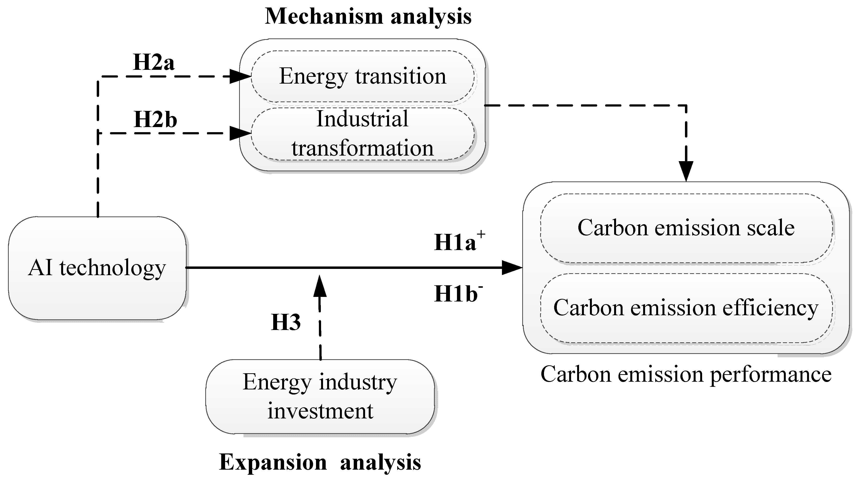
To sum up, the research framework of this paper is shown in Figure 1. This paper first tests the hypotheses H1a and H1b, i.e., the impact of AI technology on regional carbon emission performance, in which carbon emission performance is measured by the CES and CEE. Secondly, the mechanism is analyzed by using the mediation effect model, i.e., testing the hypotheses H2a and H2b from energy transition and industrial transformation. Finally, the moderating effect model is employed for expansion analysis from the perspective of energy industry investment, i.e., Hypothesis H3 is tested.

3. Econometric Model

The Stochastic Impacts by Regression on Population, Affluence, and Technology (STIRPAT) model is considered as a masterly method to investigate technology and pollution emissions [2,40,41,42,43]. The STIRPAT model has the advantage of being able to include other factors that may affect carbon emission performance through horizontal extended [30,44]. After the logarithmic, we employ the following STIRPAT model:

$$\ln I_{it}=\alpha +{\alpha }_1\ln P_{it}+{\alpha }_2\ln A_{it}+{\alpha }_3\ln T_{it}+{\gamma }_i+{\mu }_t+{\epsilon }_{it}$$

(1)

where $I_{it}$ is regional carbon emission performance of city i in year t, measured by the carbon emission scale (CES) and carbon emission efficiency (CEE); $T_{it}$ represents city i’s the standard of AI technology (AIT) in year t. Equation (1) corresponds to the research topic. Consequently, the baseline model from Equation (1) is as follows:

$$\ln CE{S}_{it}=\alpha +{\beta }_1\ln AI{T}_{it}+{\displaystyle \sum X}+{\gamma }_i+{\mu }_t+{\epsilon }_{it}$$

(2)

$$\ln CE{E}_{it}=\alpha +{\beta }_2\ln AI{T}_{it}+{\displaystyle \sum X}+{\gamma }_i+{\mu }_t+{\epsilon }_{it}$$

(3)

X represents several control variables (contains P and A in Equation (1)). ${\gamma }_i$ represents the city fixed effect, ${\mu }_t$ represents the year fixed effect, Equations (2) and (3) belong to the two-way fixed effect model (TWFE). Then, coefficients of ${\beta }_1$ and ${\beta }_2$ are the focus of this paper, indicating the impact of AI technology on carbon emission performance.

Moreover, considering the mediation effect method, this paper investigates the mechanism concerning how AI technology impacts carbon emission performance. The mechanism analysis model is as follows:

$$M{e}_{it}=\alpha +{\varphi }_1\ln AI{T}_{it}+{\displaystyle \sum X}+{\gamma }_i+{\mu }_t+{\epsilon }_{it}$$

(4)

$$\ln CE{S}_{it}=\alpha +\overline{{\beta }_1}\ln AI{T}_{it}+{\phi }_{1}M{e}_{it}+{\displaystyle \sum X}+{\gamma }_i+{\mu }_t+{\epsilon }_{it}$$

(5)

$$\ln CE{E}_{it}=\alpha +\overline{{\beta }_2}\ln AI{T}_{it}+{\phi }_{2}M{e}_{it}+{\displaystyle \sum X}+{\gamma }_i+{\mu }_t+{\epsilon }_{it}$$

(6)

Me represents the mechanism variables, which are industrial structure upgrading (IND_UP) and industrial agglomeration (IND_AGG). When the coefficients ${\varphi }_1$, ${\phi }_1$, and ${\phi }_2$ in Equations (4)–(6) are statistically significant, and the coefficient magnitude or statistical significance of $\overline{{\beta }_1}$ and $\overline{{\beta }_2}$ is lower than that of ${\beta }_1$ and ${\beta }_2$, then the mediation effect is established.

Finally, based on the moderating effect method [45], the expansion analysis of the influence of AI technology on carbon emission performance is carried out. The expansion analysis model is as follows:

$$\ln CE{S}_{it}=\alpha +{\theta }_1\ln AI{T}_{it}+{\theta }_{2}M{o}_{it}+{\theta }_3\ln AI{T}_{it}\times M{o}_{it}+{\displaystyle \sum X}+{\gamma }_i+{\mu }_t+{\epsilon }_{it}$$

(7)

$$\ln CE{E}_{it}=\alpha +{\eta }_1\ln AI{T}_{it}+{\eta }_{2}M{o}_{it}+{\eta }_3\ln AI{T}_{it}\times M{o}_{it}+{\displaystyle \sum X}+{\gamma }_i+{\mu }_t+{\epsilon }_{it}$$

(8)

Mo represents the moderating variables, which are energy industry investment (EII) and state-owned energy industry investment (SEII). When the coefficients ${\theta }_1$, ${\theta }_3$, ${\eta }_1$, and ${\eta }_3$ in Equations (7) and (8) are statistically significant, the moderating effect is recognized.

4. Data and Variables

Data from 278 Chinese cities from 2009 to 2019 are employed as research samples in this paper, with the research sample data period ending in 2019 to mitigate the systemic shock of COVID-19 outbreak on regional economic development and carbon emission. It began in 2009 in view of the lack of data on foreign direct investment and environmental regulations before 2008. The research sample data of economic and carbon emission are from the China City Statistical Yearbook, China Energy Statistical Yearbook, China Industrial Statistical Yearbook, China Agricultural Statistical Yearbook, and China Carbon Emission Accounts and Datasets (CEADs). Patent data related to AI technology were obtained from the China National Intellectual Property Administration (CNIPA). We matched patent data with economic and carbon emission data using the ZIP code of the patent application. In addition, due to lack of data on patents, economics, and carbon emissions, the inclusion excludes cities in Tibet, Hong Kong, Macao, and Taiwan. Lastly, cities with short histories (Sansha, Suizhou, and Danzhou) are not included in the research samples.

4.1. Dependent Variable

To assess the carbon emission performance, this paper utilizes the carbon emission scale (CES) and carbon emission efficiency (CEE). Under the constraint of Chinese carbon peaking and carbon neutrality, the improvement of carbon emission performance relies not only on the reduction in the CES but also on the improvement of CEE, because the reduction in carbon emissions cannot be at the expense of economic development [46]. According to Dhakal [47], Lin et al. [48], Oyewo [49], and Konadu et al. [50], a greenhouse gas emission inventory published by the World Resources Institute (WRI) and World Business Council for Sustainable Development (WBCSD) was utilized for measuring the CES in cities. According to Meng et al. [51] and Yu and Zhang [1], the Data Envelopment Analysis (DEA) method is employed to measure CEE; the details of the DEA method are shown in Appendix A.

In addition, according to Balado-Naves et al. [52] and Lin and Ma [32], employing CES per capita and CEE per capita can avoid the distraction of scale effect on carbon emission performance. The CEADs’ measurement of the CES is considered more accurate with carbon emission monitoring instruments [2,53], although there are more missing data. Consequently, CES per capita, CEE per capita, and CEADs’ carbon emission data are employed for a robustness test.

4.2. Main Independent Variables

Artificial intelligence technology (AIT). Patent representation of technological innovation is considered to be a relatively accurate and efficient method [54], and patent data are a crucial component in the identification of green technology innovation [55], energy technology innovation [56] and other industrial technology innovation by the IPC code [57]. However, it is difficult to achieve accurate recognition of AI technology by diminutively employing an IPC code [58,59,60,61]. On the one hand, AI technology has been deeply integrated with other technologies, almost completely covering all categories of patent IPC codes, and only using IPC codes to describe how AI technology may lead to over recognition [58,61]. On the other hand, the expression of the patent name of AI technology is easy to misunderstand, and it is impossible to accurately describe AI technology with the support of a patent name [59,60].

To make the identification of AI technology credible, according to Baruffaldi et al. [58] and Parteka and Kordalska [61], the keywords of the patent name and abstract combined with IPC codes are employed to identify Chinese AI technology by the number of patent applications. The keywords and IPC codes used are shown in Appendix B. Given the strictly non-negative characteristic of patent data, all types of patent data (invention and utility model) are treated as logarithmic N + 1 to avoid missing values. Moreover, to further improve the validity of patent data, the empirical results with the number of patent applications and the number of patents granted by Chinese AI technology are compared in the empirical analysis [62].

4.3. Mechanism Variables

(1) Energy transition, including energy structure cleanliness (ESC) and energy intensity (EI). A vital flag of energy transition is the energy structure cleanliness [63], i.e., the increase in the proportion of renewable or green energy in the energy structure. However, the demand for energy in economic growth is stable, so it is also necessary to consider the energy intensity, i.e., to consider whether the alternative of renewable energy to fossil energy can light the increasing energy demand [64]. Given the lack of urban renewable energy statistics in China, in accordance with Xu et al. [35] and Qu and Li [33], variable ESC is represented by the proportion of fossil energy consumption in urban total energy consumption (unit is standard coal). The decrease in this proportion indicates the improvement of the energy structure cleanliness. The EI is expressed by the percentage of urban GDP to total urban energy consumption (unit is standard coal).

(2) Industrial transformation, including industrial structure upgrading (IND_UP) and industrial agglomeration (IND_AGG). Actually, industrial structure upgrading has a strong connection with carbon emissions [65], and we need to pay attention to whether AI technology can affect carbon emission performance through industrial structure upgrading. Similarly, industrial agglomeration is also the cause of rising air pollution and carbon emissions [66].

Consequently, according to He and Zheng [67] and Zhang et al. [68], the variable of IND_UP is obtained on the basis of industrial structure rationalization (ISR) and industrial structure advancement (ISA). Specifically, the measurement of ISR is as follows:

$$IS{R}_i={\displaystyle \sum _{j=1,2,3}^n\left(\frac{Y_{ij}}{Y_i}\right)}\ln \left({\displaystyle \frac{Y_{ij}}{L_{ij}}}/{\displaystyle \frac{Y_i}{L_i}}\right)$$

(9)

where i for city, and j = 1, 2, 3 stands for primary, secondary, and tertiary industries in Chinese cities. Y is output; L is employment. The measurement of ISA is as follows:

$$IS{A}_i={\displaystyle \frac{Y_{i3}}{Y_{i2}}}$$

(10)

Generally, according to Liao et al. [69] and Zhang et al. [68], the influence of industrial structure rationalization (ISR) and industrial structure advancement (ISA) on industrial structure upgrading (IND_UP) is considered to be equally important. Then, the measurement of IND_UP is as follows:

$$IND\_U{P}_i=0.5\times IS{R}_i+0.5\times IS{A}_i$$

(11)

Finally, according to Chen et al. [66], Wang et al. [70], and Yao et al. [45], the variable of IND_AGG is measured by

$$IND\_AG{G}_i=\left(L_{ij}/{\displaystyle \sum L_{ij}}\right)/\left({\displaystyle \sum L_{ij}}/{\displaystyle \sum _i{\displaystyle \sum _j{L}_{ij}}}\right)$$

(12)

4.4. Moderating Variables

Energy industry investment (EII, SEII). The application of AI technology in the energy industry must upgrade the original equipment, methods, and processes, which depends on the energy industry investment (EII). In other words, the energy industry investment affects the depth of AI technology embedment in the energy sector. The cost of implementing AI technologies in the energy sector has a significant impact on carbon emission performance. In addition, the state-owned energy industry investment (SEII) is the main force of related financial activities. Consequently, according to Li and Li [37] and Peng et al. [26], dummy variables are constructed with the upper quartile of energy industry investment and state-owned energy industry investment to evaluate the cost of applying AI technology in the energy sector.

4.5. Control Variables

According to He and Zheng [67], Yu and Zhang [1], Zhao et al. [53], Qu and Li [33], Xu et al. [35], and Zhang et al. [2], we control for the following related variables: economic affluence (GDP), population (POP), industrial structure (IS), foreign direct investment (FDI), financial development (FD), government governance (GOV), urbanization (URB), research and development investment (RD), and environmental regulation (ER).

4.6. Descriptive Statistics

Table 2. Descriptive statistics.

	Variables	Mean	S.D.	Min	Max	Description
Dependent variable	lnAIT	3.041	1.930	0	9.436	Number of AI technology patent applications, logarithmic N + 1.
	lnAIT_granted	2.749	1.832	0	8.786	Number of AI technology patent granted, logarithmic N + 1.
Main independent variables	lnCES	8.028	0.546	6.380	11.558	Carbon emission scale, referring to Dhakal [47] and Lin et al. [48].
	lnCES_CEADs	3.329	0.913	0.294	6.126	Carbon emission scale, from https://www.ceads.net.cn/ (accessed on 1 November 2023).
	lnCEE	0.402	0.140	0.131	1.167	Carbon emission efficiency, referring to Meng et al. [51] and Yu and Zhang [1].
Control variables	lnGDP	10.585	0.625	4.595	13.056	Urban GDP per capita, logarithmic.
	lnPOP	5.913	0.649	3.784	8.136	Number of total populations, logarithmic.
	IS	0.473	0.104	0.107	0.822	Proportion of value added to tertiary industry in urban GDP.
	FDI	0.003	0.003	0	0.030	Proportion of actual utilized foreign direct investment in urban GDP.
	FD	0.950	0.604	0.118	9.622	Proportion of loans outstanding by financial institutions in urban GDP.
	GOV	0.193	0.098	0.044	1.485	Proportion of expenditure in the general budget of local governments in urban GDP.
	URB	0.533	0.152	0.151	1	Proportion of permanent urban population in total population.
	RD	0.003	0.003	0	0.063	Proportion of science and innovation spending in urban GDP.
	ER	0.003	0.001	0	0.012	Proportion of words related to environment in urban government work reports, referring to Chen et al. [71] and Qu and Li [33].
Mechanism variables	ESC	0.191	0.144	0.006	0.916	Proportion of urban fossil energy consumption to urban total energy consumption.
	EI	2.694	0.740	−1.429	5.138	The ratio of urban GDP to total urban energy consumption.
	IND_UP	0.611	0.268	0.130	2.632	Industrial structure upgrading, referring to He and Zheng [67] and Zhang et al. [68].
	IND_AGG	1.337	1.810	0.437	36.868	Industrial agglomeration, referring to Chen et al. [66] and Yao et al. [45].
Moderating variables	EII	0.455	0.498	0	1	Dummy variable, the upper quartile of the energy industry investment is shown as 1, otherwise 0.
	SEII	0.385	0.818	0	1	Dummy variable, the upper quartile of the state-owned energy industry investment is shown as 1, otherwise 0.

exhibits the descriptive statistics of major variables and reveals a few stylized facts. (1) Not all Chinese cities have carried out AI technology innovation. (2) The number difference between the applications for AI technology and those granted is small, and most of the applied AI patents are granted. (3) There is an excessive imbalance between Chinese cities in economic affluence, population, industrial structure, and urbanization. (4) Foreign direct investment, research and development investment, and environmental regulation in some Chinese cities are 0.

5. Empirical Results

5.1. Baseline Model Results

Table 3. Empirical results of baseline model.

Variables	lnCES		lnCEE
	Panel A: Measuring lnAIT by the Number of Patents Application
	(1)	(2)	(3)	(4)
lnAIT	0.0624 *** (5.46)	0.0073 ** (2.01)	−0.0085 ** (−2.53)	−0.0090 *** (−4.02)
Control variables	◯	◯	◯	◯
City fixed effect	✕	◯	✕	◯
Year fixed effect	✕	◯	✕	◯
Adj R2	0.270	0.977	0.298	0.783
Observations	3006	3006	3006	3006
Variables	lnCES		lnCEE
	Panel B: Measuring lnAIT by the Number of Patents Granted
	(1)	(2)	(3)	(4)
lnAIT_granted	0.0582 *** (4.84)	0.0071 * (1.94)	−0.0100 *** (−2.73)	−0.0078 *** (−3.34)
Control variables	◯	◯	◯	◯
City fixed effect	✕	◯	✕	◯
Year fixed effect	✕	◯	✕	◯
Adj R2	0.267	0.977	0.299	0.782
Observations	3006	3006	3006	3006

Notes: *, **, *** indicate significance levels at 10%, 5%, and 1%, respectively. The values in parentheses are t-statistic using the clustering robust standard error. ◯—considered; ✕—not considered.

reports the empirical results of Equations (1) and (2) based on pooled OLS. Panel A is the result of measuring AI technology by the number of patent applications, and Panel B is the result of measuring AI technology by the number of patents granted. Columns 1 and 3 do not consider TWFE, while columns 2 and 4 consider city and year fixed effects. Specifically, for Panel A, the coefficient of lnAIT in column 1 reaches the significance level of 1%, and the coefficient of lnAIT in column 2 is still significantly positive after controlling city and year fixed effect, which indicates that AI technology has increased the CES. Similarly, the empirical results in columns 3 and 4 show that the coefficient of lnAIT is significantly negative at 1% to 5%, which means that AI technology constrains CEE. The research hypothesis H1b is tested, not H1a.

It is evident that whether measured by the number of patent applications or the number of patents granted, AI technology has an undesirable effect on regional carbon emission performance. Generally, it is believed that technology innovation is an indispensable tool to reduce carbon emissions [72]. However, empirical results show that AI technology not only fails to reduce the CES, but also inhibits CEE. This indicates that the negative impact of AI technology on carbon emission performance outweighs its positive impact. Currently, at the macro level, AI technology has demonstrated a counterintuitive effect on carbon emission performance. Specifically, AI technology has led to an increase in CES and a decrease in CEE. Possible reasons include the following. (1) Technology implementation costs: Although AI can offer long-term energy-saving benefits, the initial investment costs may be substantial, encompassing software, hardware, and human resources. This high cost may render it unaffordable for some small- and medium-sized enterprises (SMEs), thereby limiting the widespread adoption of AI technology. (2) The carbon footprint of AI technology: The training process of certain AI models may require substantial computational resources, leading to significant carbon emissions. This could potentially offset the positive impact of these technologies on emission reduction.

5.2. Endogeneity Tests Results

It is uncertain whether AI technology affects a region’s carbon emission performance, or whether the power of carbon emission performance determines the level of AI technology. Then, reverse causality is the main cause of endogeneity issues between AI technology and carbon emission performance. To further demonstrate the robustness of the results, this paper adapts instrumental variables (IVs) and two-stage least squares (2SLS) methods to mitigate this problem. Specifically referring to Nunn and Qian [73], Liu et al. [74], Zhou (2023) [75], Zhao et al. [53], and Zhang et al. [2], these are the instrumental variables chosen in this paper: (1) The interaction term of the number of landline telephones per 100 people and the number of internet users by city in 1984. (2) The interaction term of the number of post offices per 100 people and the number of internet users by city in 1984. (3) The lagging term of AI technology. From the perspective of endogeneity, the application of AI technology relies on the backing of communication and postal infrastructure, so landline telephones and post offices have a positive correlation with AI technology. From the perspective of exogeneity, the frequency of landline telephone usage in daily life has significantly decreased, and its impact on carbon emission performance is minimal.

Table 4. The first stage of 2SLS.

Instrumental Variables	lnAIT
	(1)	(2)	(3)
lnTEL	0.1130 *** (4.45)
lnPOST		0.2641 *** (7.73)
L.lnAIT			0.7495 *** (52.81)
Control variables	◯	◯	◯
City fixed effect	◯	◯	◯
Year fixed effect	◯	◯	◯
Adj R2	0.827	0.829	0.911
Observations	2397	2397	2736

Notes: *** indicate significance levels at 1%. The values in parentheses are t-statistic using the clustering robust standard error. ◯—considered.

shows the empirical results of the first stage of 2SLS method, where the coefficients of lnTEL, lnPOST, and L.lnAIT are significantly positive, indicating that communication and postal infrastructure does contribute to improving AI technology.

Table 5. The second stage of 2SLS.

Variables	lnCES			lnCEE
	lnTEL	lnPOST	L. lnAIT	lnTEL	lnPOST	L. lnAIT
	(1)	(2)	(3)	(4)	(5)	(6)
lnAIT	0.3294 ** (2.39)	0.1507 * (1.94)	0.0817 *** (5.90)	−0.1359 *** (−3.37)	−0.1071 *** (−5.96)	−0.0136 ** (−2.07)
Control variables	◯	◯	◯	◯	◯	◯
City fixed effect	◯	◯	◯	◯	◯	◯
Year fixed effect	◯	◯	◯	◯	◯	◯
Adj R2	0.113	0.269	0.267	0.124	0.298	0.294
Observations	2397	2397	2736	2397	2397	2736

Notes: *, **, *** indicate significance levels at 10%, 5%, and 1%, respectively. The values in parentheses are t-statistic using the clustering robust standard error. ◯—considered.

shows the empirical results of the second stage of the 2SLS method. Columns 1 to 3 show the results when the dependent variable is lnCES. When the instrumental variables are lnTEL, lnPOST, and L.lnAIT, the impact of AI technology on lnCES is significantly positive at 1% to 10%, and AI technology still increases the CES. Columns 4 to 6 show the results when the dependent variable is lnCEE. It is not difficult to find that AI technology has a significantly negative impact on carbon emission efficiency, i.e., AI technology reduces CEE. The above results indicate that the main empirical results in 5.1 are still robust after the introduction of instrumental variables to mitigate the endogeneity issues caused by reverse causality.

5.3. Robustness Tests Results

5.3.1. Replace Dependent Variable

According to Balado-Naves et al. [52] and Lin and Ma [32], most economic and social activities can produce carbon emissions, which is different from other pollutants. Consequently, the employ of CES per capita and CEE per capita can alleviate the overestimation of carbon emission caused by scale effects. In addition, CEADs’ data on urban carbon emissions were used for comparison.

Table 6. Robustness tests of replacing dependent variable.

Variables	CES per Capita		CEE per Capita		lnCES_CEADs	per Capita CES_CEADs
	(1)	(2)	(3)	(4)	(5)	(6)
lnAIT	0.0623 *** (5.46)	0.0073 ** (2.00)	−0.0001 *** (−5.30)	−0.0001 *** (−2.63)	0.0168 * (1.87)	0.4964 ** (2.08)
Control variables	◯	◯	◯	◯	◯	◯
City fixed effect	✕	◯	✕	◯	◯	◯
Year fixed effect	✕	◯	✕	◯	◯	◯
Adj R2	0.551	0.986	0.646	0.930	0.953	0.893
Observations	3006	3006	3006	3006	2319	2319

Notes: *, **, *** indicate significance levels at 10%, 5%, and 1%, respectively. The values in parentheses are t-statistic using the clustering robust standard error. ◯—considered; ✕—not considered.

shows the results when CES per capita and CEE per capita are taken as dependent variables. The results in columns 1 and 2 as well as columns 5 and 6 are significantly positive, indicating that the use of CES per capita and CEADs’ data do not affect the main empirical results of this paper.

5.3.2. Consider Spatial Spillover Effects

When considering how technological innovation affects carbon emissions, it is undenied to take the spatial spillover effect of carbon emissions into account [8,76,77]. The carbon emission power of one city may affect the carbon emission performance of neighboring cities, which is determined by the physical features of CO₂ [52,78]. Consequently, the spatial econometric model is constructed to re-examine the causality between AI technology and carbon emission performance on the basis of considering the spatial spillover effect, specifically the spatial Durbin model (SDM):

$$\begin{array}{l}\ln CE{S}_{it}=\alpha +{\rho }_{1}W\ln CE{S}_{it}+{\alpha }_1\ln AI{T}_{it}+{\rho }_{2}W\ln AI{T}_{it}\\ +{\displaystyle \sum X}+{\displaystyle \sum WX}+{\gamma }_i+{\mu }_t+{\epsilon }_{it}\end{array}$$

(13)

$$\begin{array}{l}\ln CE{E}_{it}=\alpha +{\rho }_{1}W\ln CE{E}_{it}+{\alpha }_1\ln AI{T}_{it}+{\rho }_{2}W\ln AI{T}_{it}\\ +{\displaystyle \sum X}+{\displaystyle \sum WX}+{\gamma }_i+{\mu }_t+{\epsilon }_{it}\end{array}$$

(14)

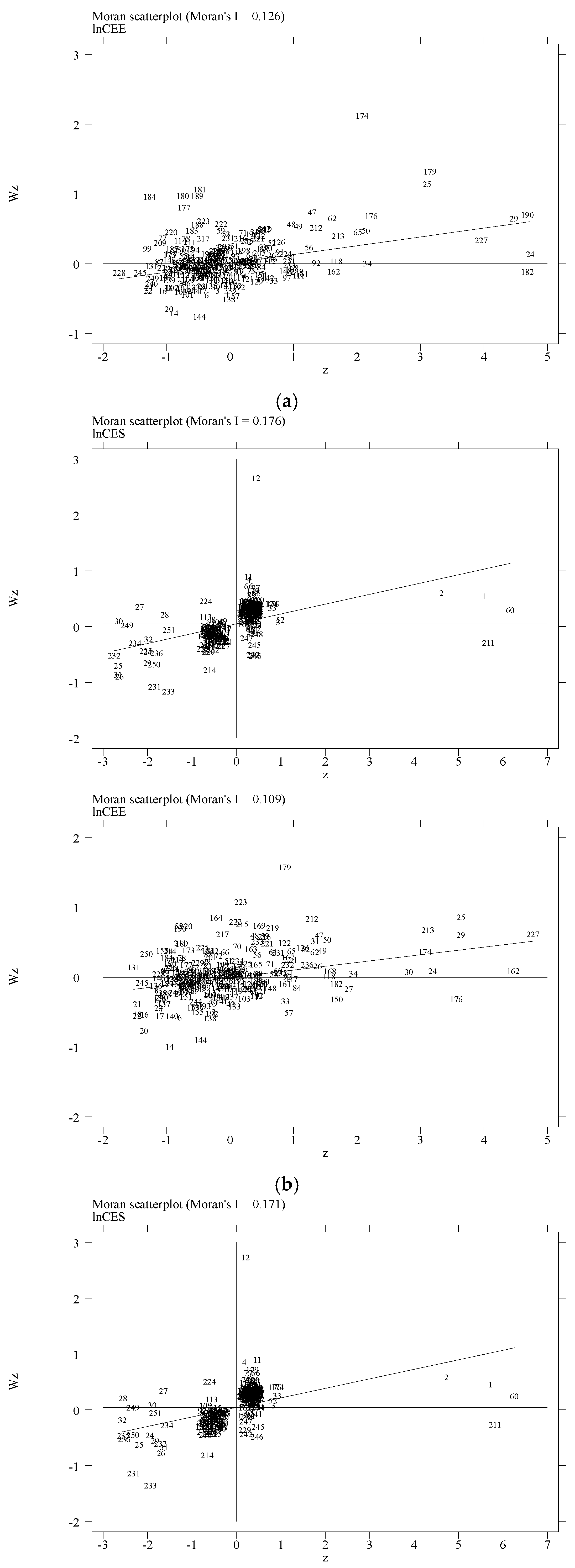
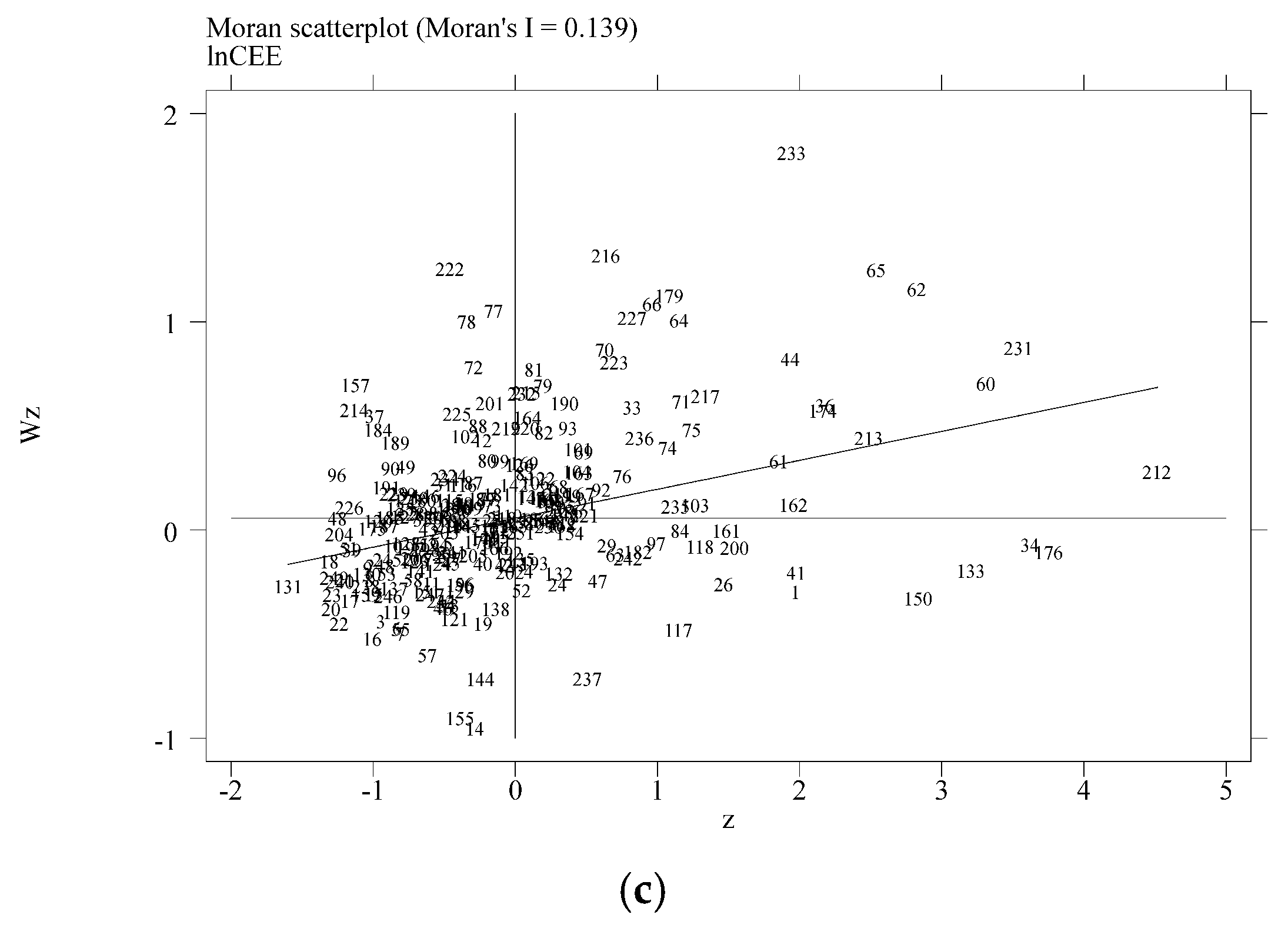
where W represents the spatial weight matrix, which is a geographic distance weight matrix (W^GEO) based on the reciprocal difference in longitude and latitude distance squared, and an economic distance weight matrix (W^ECO) based on the reciprocal difference in GDP per capita. The calculation model of the spatial weight matrix, as well as the Moran’s I scatter, employed to test the validity of the spatial econometric model, are provided in Appendix C.

Table 7. Robustness tests of consider spatial spillover effects.

Variables	lnCES		lnCEE
	WGEO	WECO	WGEO	WECO
	(1)	(2)	(3)	(4)
lnAIT	0.0074 ** (2.03)	0.0072 ** (2.01)	−0.0052 * (−1.88)	−0.0044 (−1.61)
W*lnAIT	0.0006 (0.05)	−0.0033 (−0.48)	−0.0157 * (−1.81)	−0.0208 *** (−3.89)
Spatial rho ($\rho$)	0.0968 * (1.88)	0.0821 *** (2.63)	0.3179 *** (7.33)	0.2552 *** (9.60)
Variance sigma2_e	0.0058 *** (33.59)	0.0058 *** (33.58)	0.0034 *** (33.46)	0.0034 *** (33.42)
Control variables	◯	◯	◯	◯
Control variables (W)	◯	◯	◯	◯
City fixed effect	◯	◯	◯	◯
Year fixed effect	◯	◯	◯	◯
Observations	2259	2259	2259	2259

Notes: *, **, *** indicate significance levels at 10%, 5%, and 1%, respectively. The values in parentheses are t-statistic using the clustering robust standard error. W represents the spatial weight matrix. ◯—considered.

shows the impact of AI technology on regional carbon emission performance after considering spatial spillover effect. Specifically, the spatial lag coefficient ($\rho$) is significantly positive, which proves that there is a spatial spillover effect between the carbon emission scale (lnCES) and carbon emission efficiency (lnCEE). The coefficient of lnAIT in column 1 and column 2 is significantly positive, while the coefficient of W*lnAIT is not significant, which indicates that AI technology still improves the CES even considering spatial spillover effect, and this effect is in local cities. The coefficient of lnAIT in column 3 is significantly negative, and the coefficients of W*lnAIT in column 3 and column 4 are also significantly negative, which means that if the spatial spillover effect is considered in lnCEE, the undesirable effect of AI technology on CEE not only comes from the local cities, but also is affected by neighboring cities. In general, even considering the spatial spillover effect, the results in Table 7 have not reformed greatly compared with Table 3, and the conclusions in this paper are robust.

5.3.3. Time Sensitivity of Sample Data

The financial crisis that occurred worldwide in 2008 and the outbreak of COVID-19 in 2019, which suppressed economic activity and produced additional carbon reduction effects, may have overrated the impact of AI technologies on carbon emission performance. Thus, according to Zhang et al. [2], transformation of the period for sample data in the baseline model is 2011–2017 in order to re-examine the impact of AI technology on carbon emission performance. The results of columns 1 and 2 in

Table 8. Robustness tests of time sensitivity.

Variables	lnCES		lnCEE
	(1)	(2)	(3)	(4)
lnAIT	0.0630 *** (4.56)	0.0092 * (1.91)	−0.0128 *** (−3.94)	−0.0062 *** (−2.65)
Control variables	◯	◯	◯	◯
City fixed effect	✕	◯	✕	◯
Year fixed effect	✕	◯	✕	◯
Adj R2	0.269	0.977	0.269	0.854
Observations	1922	1921	1922	1921

Notes: *, *** indicate significance levels at 10% and 1%, respectively. The values in parentheses are t-statistic using the clustering robust standard error. ◯—considered; ✕—not considered.

show that when the dependent variable is lnCES, the coefficient of lnAIT is significantly positive, i.e., AI technology increases the CES. The results in columns 3 and 4 show that AI technology still reduces CEE. It is obvious that changing the period of sample data does not affect the causality between AI technology and carbon emission performance, and the results of this paper are robust.

5.3.4. Change the Estimation Method

According to Huang et al. [41], Parteka and Kordalska [61], and Vélez-Henao et al. [42], we re-estimate Equations (2) and (3) based on the system generalized method of moment (sys-GMM) and difference generalized method of moment (diff-GMM) methods. The results of sys-GMM and diff-GMM estimation are reported in

Table 9. Robustness tests of change to the model estimation method.

Variables	lnCES		CES per Capita
	diff-GMM	sys-GMM	diff-GMM	sys-GMM
	(1)	(2)	(3)	(4)
lnAIT	0.0205 *** (4.64)	0.0148 *** (3.24)	0.0218 *** (4.92)	0.0168 *** (3.75)
L. lnCES	0.2172 *** (3.56)	0.2489 *** (6.25)
L. per capita CES			0.2161 *** (3.25)	0.2010 *** (4.91)
Control variables	◯	◯	◯	◯
AR (1)_P	0.000	0.000	0.000	0.000
AR (2)_P	0.230	0.158	0.201	0.142
Observations	2456	2736	2456	2736

Notes: *** indicate significance levels at 1%. The values in parentheses are t-statistic using the clustering robust standard error. AR (1) and AR (2) are the P value for the first- or second-order autocorrelations tests. ◯—considered.

. Specifically, the coefficient of lnAIT in columns 1 to 4 is significantly positive at the 1%, indicating that AI technology increases the CES, and the undesired effect of AI technology still exists even when the scale effect is considered.

5.3.5. Policy Competition Effect

Carbon emission performance is inevitably influenced by regional environmental policies, so it is imperative to take the possible competition effects of environmental policies into account. Specifically, according to Lee and Nie [55] and Qu and Li [33], we exclude the sample of municipalities and consider the impact of the Low Carbon City Pilot (LCCP) and Carbon Emission Trading Pilot (CETP), environmental policies that are highly correlated with carbon emissions, on carbon emission performance. The results of

Table 10. Robustness tests of policy competition effect.

Variables	lnCES			lnCEE
	Exclude the Municipalities	Control the LCCP	Control the CETP	Exclude the Municipalities	Control the LCCP	Control the CETP
	(1)	(2)	(3)	(4)	(5)	(6)
lnAIT	0.0073 ** (2.03)	0.0060 * (1.86)	0.0072 ** (1.99)	−0.0085 *** (−3.84)	−0.0088 *** (−3.93)	−0.0088 *** (−3.95)
LCCP		0.0004 (0.07)			−0.0004 (−0.07)
CETP			0.0061 (1.03)			−0.0133 * (−1.69)
Control variables	◯	◯	◯	◯	◯	◯
City fixed effect	◯	◯	◯	◯	◯	◯
Year fixed effect	◯	◯	◯	◯	◯	◯
Adj R2	0.957	0.977	0.977	0.785	0.784	0.783
Observations	2962	2962	3006	2962	2962	3006

Notes: *, **, *** indicate significance levels at 10%, 5%, and 1%, respectively. The values in parentheses are t-statistic using the clustering robust standard error. ◯—considered.

show that after excluding municipalities in columns 1 and 4, the impact of AI technology on carbon emission performance is aligned with the results of the baseline model in Table 3. Similarly, columns 2 and 5, as well as columns 3 and 6, respectively, show the impact of AI technology on carbon emission performance after controlling LCCP and CETP environmental policies, and the results are still analogical to Table 3.

5.3.6. Changing Clustering and Fixed Effects

According to Zhang et al. [2], the influence range of clustering and fixed effects is changed to control the factors affecting carbon emission performance at the provincial level. The results of

Table 11. Robustness tests of changing clustering and fixed effects.

Variables	lnCES			lnCEE
	(1)	(2)	(3)	(4)	(5)	(6)
lnAIT	0.0624 ** (2.03)	0.0073 ** (2.09)	0.0091 ** (2.45)	−0.0085 ** (−2.37)	−0.0090 *** (−3.41)	−0.0045 * (−1.85)
Control variables	◯	◯	◯	◯	◯	◯
Province × Year fixed effect	✕	✕	◯	✕	✕	◯
Province fixed effect	✕	◯	✕	✕	◯	✕
City fixed effect	✕	◯	◯	✕	◯	◯
Year fixed effect	✕	◯	◯	✕	◯	◯
Cluster to city	◯	◯	◯	◯	◯	◯
Adj R2	0.270	0.977	0.957	0.298	0.780	0.819
Observations	3006	3006	2940	3006	3006	2940

Notes: *, **, *** indicate significance levels at 10%, 5%, and 1%, respectively. The values in parentheses are t-statistic using the clustering robust standard error. ◯—considered; ✕—not considered.

in columns 1 to 3 show that the coefficient of lnAIT is significantly positive, while the results in columns 4 to 6 show that the coefficient of lnAIT is significantly negative; in other words, changing the influence range of clustering and fixed effects, AI technology is still not conducive to carbon emission performance.

5.4. Mechanism Analysis Results

The purpose of mechanism analysis is to explore the channels through which AI technology affects carbon emission performance. The mechanism analysis is based on Equations (4)–(6), while

Table 12. (a) Mechanism analysis of energy transition. (b) Mechanism analysis of energy transition in the Yangtze River Economic Belt. (c) Mechanism analysis of energy transition in the Heihe–Tengchong Line (southeast).

(a)
Variables	esc	lnCES	lnCEE	ei	lnCES	lnCEE
	(1)	(2)	(3)	(4)	(5)	(6)
lnAIT	−0.0059 ** (2.13)	0.0070 * (1.92)	−0.0086 *** (−3.84)	−0.0255 * (−1.76)	0.0073 ** (1.98)	−0.0081 *** (−3.70)
ESC		−0.0491 ** (1.97)	0.0802 *** (3.93)
EI					−12.7240 ** (−2.12)	−3.0551 *** (−2.78)
Control variables	◯	◯	◯	◯	◯	◯
City fixed effect	◯	◯	◯	◯	◯	◯
Year fixed effect	◯	◯	◯	◯	◯	◯
Adj R2	0.757	0.977	0.784	0.778	0.977	0.792
Observations	2984	2984	2984	2984	2984	2984
(b)
Variables	esc	lnCES	lnCEE	ei	lnCES	lnCEE
	(1)	(2)	(3)	(4)	(5)	(6)
lnAIT	−0.0042 (−1.15)	0.0091 (1.47)	−0.0080 ** (−2.20)	−0.0541 *** (−2.77)	0.0089 (1.44)	−0.0052 (−1.49)
ESC		0.0118 (0.33)	0.0457 (1.30)
EI					−0.0030 (−0.29)	0.0547 *** (7.96)
Control variables	◯	◯	◯	◯	◯	◯
City fixed effect	◯	◯	◯	◯	◯	◯
Year fixed effect	◯	◯	◯	◯	◯	◯
Adj R2	0.805	0.979	0.799	0.753	0.979	0.814
Observations	1185	1185	1185	1185	1185	1185
(c)
Variables	esc	lnCES	lnCEE	ei	lnCES	lnCEE
	(1)	(2)	(3)	(4)	(5)	(6)
lnAIT	−0.0061 ** (−2.12)	0.0078 ** (2.32)	−0.0087 *** (−4.12)	−0.0273 * (−1.94)	0.0078 ** (2.34)	−0.0081 *** (−3.85)
ESC		−0.0325 (−1.55)	0.0570 *** (2.74)
EI					−0.0065 (−1.31)	0.0370 *** (8.81)
Control variables	◯	◯	◯	◯	◯	◯
City fixed effect	◯	◯	◯	◯	◯	◯
Year fixed effect	◯	◯	◯	◯	◯	◯
Adj R2	0.765	0.979	0.781	0.757	0.979	0.788
Observations	2787	2787	2787	2787	2787	2787

Notes: *, **, *** indicate significance levels at 10%, 5%, and 1%, respectively. The values in parentheses are t-statistic using the clustering robust standard error. ◯—considered.

a–c and

Table 13. (a) Mechanism analysis of industrial transformation. (b) Mechanism analysis of industrial transformation in the Yangtze River Economic Belt. (c) Mechanism analysis of industrial transformation in the Heihe–Tengchong Line (southeast).

(a)
Variables	ind_up	lnCES	lnCEE	ind_agg	lnCES	lnCEE
	(1)	(2)	(3)	(4)	(5)	(6)
lnAIT	0.0014 (0.52)	0.0076 ** (2.08)	−0.0094 *** (−4.19)	0.0431 (1.23)	0.0077 ** (2.07)	−0.0091 *** (−4.07)
IND_UP		−0.0038 (−0.16)	0.0255 (1.08)
IND_AGG					−0.0019 (−1.23)	−0.0062 *** (−6.41)
Control variables	◯	◯	◯	◯	◯	◯
City fixed effect	◯	◯	◯	◯	◯	◯
Year fixed effect	◯	◯	◯	◯	◯	◯
Adj R2	0.921	0.977	0.782	0.788	0.977	0.783
Observations	2918	2918	2918	2919	2919	2919
(b)
Variables	ind_up	lnCES	lnCEE	ind_agg	lnCES	lnCEE
	(1)	(2)	(3)	(4)	(5)	(6)
lnAIT	−0.0102 ** (−2.34)	0.0077 (1.21)	−0.0099 *** (−2.81)	0.0013 (0.19)	0.0079 (1.25)	−0.0106 *** (−3.00)
IND_UP		−0.0350 (−0.64)	0.0780 (1.36)
IND_AGG					0.0391 (1.20)	0.0002 (0.01)
Control variables	◯	◯	◯	◯	◯	◯
City fixed effect	◯	◯	◯	◯	◯	◯
Year fixed effect	◯	◯	◯	◯	◯	◯
Adj R2	0.914	0.979	0.797	0.455	0.979	0.795
Observations	1148	1148	1148	1149	1149	1149
(c)
Variables	ind_up	lnCES	lnCEE	ind_agg	lnCES	lnCEE
	(1)	(2)	(3)	(4)	(5)	(6)
lnAIT	−0.0006 (−0.20)	0.0080 ** (2.38)	−0.0095 *** (−4.51)	0.0445 (1.16)	0.0081 ** (2.38)	−0.0092 *** (−4.42)
IND_UP		−0.0076 (−0.31)	0.0317 (1.15)
IND_AGG					−0.0021 (−1.45)	−0.0063 *** (−5.98)
Control variables	◯	◯	◯	◯	◯	◯
City fixed effect	◯	◯	◯	◯	◯	◯
Year fixed effect	◯	◯	◯	◯	◯	◯
Adj R2	0.926	0.979	0.780	0.784	0.979	0.782
Observations	2724	2724	2724	2725	2725	2725

Notes: **, *** indicate significance levels at 5% and 1%, respectively. The values in parentheses are t-statistic using the clustering robust standard error. ◯—considered.

a–c show the mechanism analysis of energy transition and industrial transformation, respectively.

Specifically, column 1 of Table 12a reports the coefficient of the lnAIT, which is significantly negative, pointing out that AI technology reduces the proportion of fossil fuels in total energy consumption. Further, the coefficient of the esc in columns 2 and 3 is significant, and the coefficient of the lnAIT is reduced or less significant than that in columns 2 and 4 of Table 3. Consequently, the mediation effect of esc is established, i.e., AI technology improves the CES and CEE by reducing the proportion of fossil fuels in total energy consumption. Similarly, the empirical results in columns 5 and 6 indicate that the mediation effect of EI is also established, i.e., AI technologies affect the CES and CEE by reducing EI. Table 12b,c discuss the mechanism of energy transition in the context of typical geographical locations (Yangtze River Economic Belt, Heihe–Tengchong Line). In terms of the Yangtze River Economic Belt, the mechanism of energy transition is not established, which means that the Yangtze River Economic Belt is not the most widely applied AI technology in China. However, the results for the Heihe–Tengchong Line are largely consistent with those presented in Table 12a. It is evident that the southeast side of the Heihe–Tengchong Line encompasses over 90% of the observed cities, which are clearly the most significant sources of carbon emissions in China. Commonly, AI technology can affect regional carbon emission performance through ESC and EI, in other words, AI technology has the potential to improve regional carbon emission performance by influencing energy transition.

Table 13a shows the mechanism analysis results of industrial transformation. The coefficient of lnAIT in column 1 and column 4 is positive but not significant, indicating that AI technology has nothing to do with industrial structure upgrading and agglomeration, so the mediation effect of variables IND_UP and IND_AGG is not valid. The channel which AI technology affects carbon emission performance is not industrial structure upgrading and industrial agglomeration, and the influence of AI technology at the Chinese industry is undefined. Table 13b,c show similar results. In other words, even when accounting for certain special industries and economically developed regions, AI technology remains unable to influence carbon emissions through industrial transformation. From a macro perspective, the penetration of artificial intelligence technology in the process of industrial transformation remains insufficient. Of course, AI technology is already widely employed in specific industries (such as information transmission, software, and information technology services). The impact of AI technologies on the carbon emission performance of specific industries may be observed with micro-level firm data. The research hypothesis H2a is tested, not H2b.

5.5. Expansion Analysis Results

The purpose of the expansion analysis is to describe why AI technology is harmful to carbon emission performance from the perspective of energy industry investment. Generally, the energy sector is not the ‘birthplace’ of AI technology, so the application of AI technology in the energy sector may need to pay additional cost, which will result in a boost in energy industry investment, thus affecting carbon emissions [37]. In other words, under the prerequisite of high energy industry investment, the adverse impact of AI technology may be more prominent, and the vital obstacle for AI technology to save energy and reduce emission is the increasing investment in energy industry. Consequently, to find out the explanations why AI technology is unfavorable for carbon emission performance at present, according to Ahmad et al. [79] and Peng et al. [26], we perform an expansion analysis from the perspective of energy industry investment.

Table 14. (a) Expansion analysis of energy industry investment. (b) Expansion analysis of energy industry investment in the Yangtze River Economic Belt. (c) Expansion analysis of energy industry investment in the Heihe–Tengchong Line (southeast).

(a)
Variables	lnCES	lnCEE	lnCES	lnCEE
	(1)	(2)	(3)	(4)
lnAIT	0.0064 * (1.76)	−0.0109 *** (−4.84)	0.0049 (1.29)	−0.0099 *** (−4.00)
lnAIT×EII	0.0020 * (1.87)	0.0042 *** (4.22)
lnAIT×SEII			0.0027 ** (2.22)	0.0010 (0.84)
Control variables	◯	◯	◯	◯
City fixed effect	◯	◯	◯	◯
Year fixed effect	◯	◯	◯	◯
Adj R2	0.977	0.784	0.977	0.783
Observations	3006	3006	3006	3006
(b)
Variables	lnCES	lnCEE	lnCES	lnCEE
	(1)	(2)	(3)	(4)
lnAIT	0.0082 (1.34)	−0.0098 *** (−2.77)	0.0051 (0.81)	−0.0110 *** (−2.86)
lnAIT×EII	0.0041 ** (2.00)	0.0077 *** (4.26)
lnAIT×SEII			0.0048 ** (2.46)	0.0034 ** (2.02)
Control variables	◯	◯	◯	◯
City fixed effect	◯	◯	◯	◯
Year fixed effect	◯	◯	◯	◯
Adj R2	0.979	0.803	0.979	0.799
Observations	1185	1185	1185	1185
(c)
Variables	lnCES	lnCEE	lnCES	lnCEE
	(1)	(2)	(3)	(4)
lnAIT	0.0074 ** (2.22)	−0.0109 *** (−5.15)	0.0062 * (1.79)	−0.0101 *** (−4.32)
lnAIT×EII	0.0013 (1.34)	0.0043 *** (4.19)
lnAIT×SEII			0.0020 * (1.89)	0.0012 (1.01)
Control variables	◯	◯	◯	◯
City fixed effect	◯	◯	◯	◯
Year fixed effect	◯	◯	◯	◯
Adj R2	0.978	0.782	0.979	0.780
Observations	2809	2809	2809	2809

Notes: *, **, *** indicate significance levels at 10%, 5%, and 1%, respectively. The values in parentheses are t-statistic using the clustering robust standard error. ◯—considered.

a shows the results of expansion analysis when the dependent variables are the CES and CEE, respectively. The coefficients of lnAIT, lnAIT×EII, and lnAIT×SEII in column 1 and column 3 are positive, pointing out that energy industry investment (EII and SEII) shows a positive moderating effect between AI technology and the CES. The results in column 2 and 4 show that the coefficient of lnAIT is significantly negative, and the coefficients of lnAIT×EII and lnAIT×SEII are positive, which also means that energy industry investment has a positive responsibility for the impact of AI technology on CEE. The results in Table 14c are consistent with those in Table 14a, indicating that AI technology plays a more significant role in enhancing CEE. However, the results presented in Table 14b indicate that for the Yangtze River Economic Belt, a specific economic zone with significant environmental relevance, the moderating effect of energy industry investment is more pronounced (0.0041 > 0.0020, 0.0077 > 0.0042). Strengthening the application of AI technology in the energy sector within this region can facilitate the realization of its emission reduction potential.

It is not difficult to find that to employ AI technology in the energy sector requires increased investment in the energy industry to improve equipment, method, and processes, which will increase costs, and in turn affect the CES and CEE. In other words, current investments in the energy industry are not improving the application and carbon emission performance of AI technologies in the energy sector. The research hypothesis H3 is tested.

5.6. Heterogeneity Analysis Results

Intellectual property protection affects the development and spillover of AI technologies, and digital infrastructure is crucial to determining the impact of AI technologies. Consequently, this paper analyzes the potential heterogeneity issue of AI technology in affecting carbon emission performance from the perspectives of intellectual property protection, digital infrastructure, patent types, and region. Specifically, according to Hao et al. [80], the level of intellectual property protection is measured by the median of patent infringement cases closed in cities to the total number of patent infringement cases closed in China. The level of digital infrastructure is measured by the median of the ratio of internet broadband access ports to population. Patent types are divided into invention patents and utility model patents. Regional heterogeneity is considered in the east and west and the Yangtze River Economic Belt (YREB).

Table 15. Heterogeneity analysis of intellectual property protection.

Variables	lnCES		lnCEE
	High	Low	High	Low
	(1)	(2)	(3)	(4)
lnAIT	0.0096 * (1.70)	0.0111 * (1.90)	−0.0046 (−1.41)	−0.0070 ** (−2.20)
Control variables	◯	◯	◯	◯
City fixed effect	◯	◯	◯	◯
Year fixed effect	◯	◯	◯	◯
Adj R2	0.976	0.976	0.822	0.821
Observations	1749	1255	1749	1255

Notes: *, ** indicate significance levels at 10% and 5%, respectively. The values in parentheses are t-statistic using the clustering robust standard error. ◯—considered.

reports the heterogeneity of intellectual property protection. The coefficients of lnAIT in columns 2 and 4 are larger than those of lnAIT in columns 1 and 3 in both statistical significance and scale, indicating that AI technologies are less friendly to carbon emission performance in regions with lower planes of intellectual property protection.

Table 16. Heterogeneity analysis of digital infrastructure.

Variables	lnCES		lnCEE
	High	Low	High	Low
	(1)	(2)	(3)	(4)
lnAIT	0.0109 * (1.70)	0.0092 * (1.80)	−0.0052 (−1.48)	−0.0036 ** (−2.38)
Control variables	◯	◯	◯	◯
City fixed effect	◯	◯	◯	◯
Year fixed effect	◯	◯	◯	◯
Adj R2	0.978	0.975	0.836	0.861
Observations	1633	1372	1633	1372

Notes: *, ** indicate significance levels at 10% and 5%, respectively. The values in parentheses are t-statistic using the clustering robust standard error. ◯—considered.

shows the heterogeneity analysis of digital infrastructure. Regions with weak digital infrastructure experience a greater negative impact of AI technology on CEE.

Table 17. Heterogeneity analysis of patent type.

Variables	lnCES		lnCEE
	Invention	Utility Model	Invention	Utility Model
	(1)	(2)	(3)	(4)
lnAIT	0.0060 * (1.70)	0.0063 ** (2.05)	−0.0048 ** (−2.16)	−0.0059 *** (−2.60)
Control variables	◯	◯	◯	◯
City fixed effect	◯	◯	◯	◯
Year fixed effect	◯	◯	◯	◯
Adj R2	0.977	0.977	0.782	0.782
Observations	3006	3006	3006	3006

Notes: *, **, *** indicate significance levels at 10%, 5%, and 1%, respectively. The values in parentheses are t-statistic using the clustering robust standard error. ◯—considered.

shows the heterogeneity analysis results of patent types. Compared with invention patents, utility model patents of AI technology have a more unfavorable effect on carbon emission performance. In other words, low innovation quality AI technology is bad for the environment. Finally,

Table 18. Heterogeneity analysis of region (lnCES).

Variables	lnCES
	Eastern	Central	Western	YREB	Non-YREB
	(1)	(2)	(3)	(4)	(5)
lnAIT	0.0040 (0.96)	0.0053 (1.23)	0.0153 *** (2.65)	0.0090 (1.47)	0.0063 (1.40)
Control variables	◯	◯	◯	◯	◯
City fixed effect	◯	◯	◯	◯	◯
Year fixed effect	◯	◯	◯	◯	◯
Adj R2	0.989	0.920	0.970	0.979	0.976
Observations	1099	1085	822	1185	1821

Notes: *** indicate significance levels at 1%. The values in parentheses are t-statistic using the clustering robust standard error. ◯—considered.

and

Table 19. Heterogeneity analysis of region (lnCEE).

Variables	lnCEE
	Eastern	Central	Western	YREB	Non-YREB
	(1)	(2)	(3)	(4)	(5)
lnAIT	−0.0214 *** (−4.71)	−0.0062 ** (−2.52)	−0.0054 (−1.13)	−0.0082 ** (−2.27)	−0.0086 *** (−2.94)
Control variables	◯	◯	◯	◯	◯
City fixed effect	◯	◯	◯	◯	◯
Year fixed effect	◯	◯	◯	◯	◯
Adj R2	0.771	0.830	0.793	0.798	0.776
Observations	1099	1085	822	1185	1821

Notes: **, *** indicate significance levels at 5% and 1%, respectively. The values in parentheses are t-statistic using the clustering robust standard error. ◯—considered.

show the results of the analysis of regional heterogeneity. For the CES, the impact of AI technology is more prominent in the western, but not in the non-western region. For CEE, the negative impact caused by AI technology is mainly reflected in the eastern and central regions, which is contrary to the CES. For the Yangtze River Economic Belt (YREB), the undesirable effect AI technology on CEE is relatively low, but it is still significant.

6. Conclusions and Policy Implications

It is believed that AI technology can enhance energy efficiency, decrease carbon footprint, and improve energy management, which would be advantageous for carbon emission performance. However, the use of AI technology may also increase energy consumption and additional cost inputs, which may be detrimental to carbon emission performance. To verify the impact of AI technology on carbon emission performance, this paper conducted an empirical analysis based on the data of 278 Chinese cities from 2009 to 2019, as well as AI technologies considered by a combination of IPC codes and keyword searches. The empirical results show that (1) AI technology not only increases the CES, but also reduces the CEE, which indicates that current AI technology does not necessarily improve carbon emission performance. Energy transition is a channel through which AI technology affects carbon emission performance. Specifically, AI technology has the potential to optimize carbon emission performance by reducing the proportion of fossil energy consumption and reducing energy intensity. (2) Energy industry investment plays a positive regulatory role in the impact of AI technology on carbon emission performance, i.e., energy industry investment intensifies the undesirable effect of AI technology on carbon emission performance. (3) In regions with low innovation quality and low intellectual property protection, the negative impact of AI technology on carbon emission performance is evident, as demonstrated by heterogeneity analysis.

Overall, the role of the energy transition is critical if AI technologies are to have a positive impact on carbon emission performance. Not only is the generation of carbon emissions high connected to the energy sector, but AI technology is an important way to transform the old energy sector to balance productivity and green development. Given the failure of current AI technology to reduce carbon emission, the policy implications are as follows:

Firstly, targeted voluntary environmental policies should be utilized to stimulate innovation in the energy sector by firms with advantages in AI technology. We advocate reinforcing the application of AI technology in the energy sector and environmental protection, developing AI technologies with distinctive characteristics specific to the energy sector, such as intelligent exploration and renewable energy integration. This will facilitate the deep integration of AI technology in the energy sector.

Secondly, based on command-and-control environmental policies, high energy consumption firms are forced to carry out technological transition to green, forcing them to actively apply AI technology, and truly play the advantages of AI technology in efficiency and cost. Companies in the energy sector should not only focus on the productivity impacts of AI technology but also prioritize its carbon reduction effects.

Thirdly, we should further adopt market-based environmental policies to mitigate the aggravating effect of energy industry investment on carbon emission performance, and give more financial support to the application of AI technology in the energy sector. To realize the carbon reduction effect of AI technology, reducing the application cost of AI technology and enhancing the innovation quality of AI technology though market mechanism is of the same necessity.

References

- Yu, Y.; Zhang, N. Low-carbon city pilot and carbon emission efficiency: Quasi-experimental evidence from China. Energy Econ. 2021, 96, 105125. [Google Scholar] [CrossRef]
- Zhang, W.; Liu, X.; Wang, D.; Zhou, J. Digital economy and carbon emission performance: Evidence at China’s city level. Energy Policy 2022, 165, 112927. [Google Scholar] [CrossRef]
- Ding, T.; Li, J.; Shi, X.; Li, X.; Chen, Y. Is artificial intelligence associated with carbon emissions reduction? Case of China. Resour. Policy 2023, 85, 103892. [Google Scholar] [CrossRef]
- Ganda, F. The impact of innovation and technology investments on carbon emissions in selected organisation for economic Co-operation and development countries. J. Clean. Prod. 2019, 217, 469–483. [Google Scholar] [CrossRef]
- Ghoddusi, H.; Creamer, G.G.; Rafizadeh, N. Machine learning in energy economics and finance: A review. Energy Econ. 2019, 81, 709–727. [Google Scholar] [CrossRef]
- Luccioni, A.; Lacoste, A.; Schmidt, V. Estimating Carbon Emissions of Artificial Intelligence. IEEE Technol. Soc. Mag. 2020, 39, 48–51. [Google Scholar] [CrossRef]
- Ye, Z.; Yang, J.; Zhong, N.; Tu, X.; Jia, J.; Wang, J. Tackling environmental challenges in pollution controls using artificial intelligence: A review. Sci. Total Environ. 2020, 699, 134279. [Google Scholar] [CrossRef]
- Chen, Y.; Cheng, L.; Lee, C.C. How does the use of industrial robots affect the ecological footprint? International evidence. Ecol. Econ. 2022, 198, 107483. [Google Scholar] [CrossRef]
- Chen, C.; Hu, Y.; Marimuthu, K.; Kumar, P.M. Artificial intelligence on economic evaluation of energy efficiency and renewable energy technologies. Sustain. Energy Technol. Assess. 2021, 47, 101358. [Google Scholar] [CrossRef]
- Huang, G.; He, L.Y.; Lin, X. Robot adoption and energy performance: Evidence from Chinese industrial firms. Energy Econ. 2022, 107, 105837. [Google Scholar] [CrossRef]
- Gaur, L.; Afaq, A.; Arora, G.K.; Khan, N. Artificial intelligence for carbon emissions using system of systems theory. Ecol. Inform. 2023, 76, 102165. [Google Scholar] [CrossRef]
- Liu, Z.; Zhong, J.; Liu, Y.; Liang, Y.; Li, Z. Dynamic simulation of street-level carbon emissions in megacities: A case study of wuhan city, china (2015–2030). Sustain. Cities Soc. 2024, 115, 105853. [Google Scholar] [CrossRef]
- Xia, M.; Dong, L.; Zhao, X.; Jiang, L. Green technology innovation and regional carbon emissions: Analysis based on heterogeneous treatment effect modeling. Environ. Sci. Pollut. Res. 2024, 31, 9614–9629. [Google Scholar] [CrossRef] [PubMed]
- Chen, Y.; Jin, S. Artificial intelligence and carbon emissions in manufacturing firms: The moderating role of green innovation. Processes 2023, 11, 2705. [Google Scholar] [CrossRef]
- Hou, J.; Kang, W.; Li, Y.; Liang, S.; Geng, S. Does Digital-Intelligence Contribute to Carbon Emission Reduction? New Insights from China. SAGE Open 2024, 14, 21582440241304462. [Google Scholar] [CrossRef]
- Su, L.; Ji, T.; Ahmad, F.; Chandio, A.A.; Ahmad, M.; Jabeen, G.; Rehman, A. Technology innovations impact on carbon emission in Chinese cities: Exploring the mediating role of economic growth and industrial structure transformation. Environ. Sci. Pollut. Res. 2023, 30, 46321–46335. [Google Scholar] [CrossRef]
- Liu, Z.; Du, S.; Zhang, L.; Xie, J.; Wang, X. Does the coupling of digital and green technology innovation matter for carbon emissions? J. Environ. Manag. 2025, 373, 123824. [Google Scholar] [CrossRef]
- Chen, X.; Mao, S.; Lv, S.; Fang, Z. A study on the non-linear impact of digital technology innovation on carbon emissions in the transportation industry. Int. J. Environ. Res. Public Health 2022, 19, 12432. [Google Scholar] [CrossRef]
- Pu, Z.; Qian, Y.; Liu, R. Is digital technology innovation a panacea for carbon reduction? Technol. Econ. Dev. Econ. 2024, 1–29. [Google Scholar] [CrossRef]
- Jiang, Y.; Zhao, R.; Qin, G. How does digital finance reduce carbon emissions intensity? Evidence from chain mediation effect of production technology innovation and green technology innovation. Heliyon 2024, 10, e30155. [Google Scholar] [CrossRef]
- Du, M.; Zhou, Q.; Zhang, Y.; Li, F. Towards sustainable development in China: How do green technology innovation and resource misallocation affect carbon emission performance? Front. Psychol. 2022, 13, 929125. [Google Scholar] [CrossRef] [PubMed]
- Dong, H.; Yan, Z.; Zhang, J. Does green technology innovation improve carbon emission efficiency? Evidence from energy-intensive enterprises in China. Environ. Dev. Sustain. 2024, 1–33. [Google Scholar] [CrossRef]
- Abdalla, A.N.; Nazir, M.S.; Tao, H.; Cao, S.; Ji, R.; Jiang, M.; Yao, L. Integration of energy storage system and renewable energy sources based on artificial intelligence: An overview. J. Energy Storage 2021, 40, 102811. [Google Scholar] [CrossRef]
- Dileep, G. A survey on smart grid technologies and applications. Renew. Energy 2020, 146, 2589–2625. [Google Scholar] [CrossRef]
- Stern, N.; Valero, A. Research policy, Chris Freeman special issue innovation, growth and the transition to net-zero emissions. Res. Policy 2021, 50, 104293. [Google Scholar] [CrossRef]
- Peng, J.; Xiao, J.; Wen, L.; Zhang, L. Energy industry investment influences total factor productivity of energy exploitation: A biased technical change analysis. J. Clean. Prod. 2019, 237, 117847. [Google Scholar] [CrossRef]
- Aghion, P.; Jones, B.F.; Jones, C.I. Artificial Intelligence and Economic Growth; National Bureau of Economic Research: Cambridge, MA, USA, 2017; Volume 23928. [Google Scholar] [CrossRef]
- Soofastaei, A. The Application of Artificial Intelligence to Reduce Greenhouse Gas Emissions in the Mining Industry. In Green Technologies to Improve the Environment on Earth; Pacheco, M., Ed.; IntechOpen: Rijeka, Croatia, 2018; Chapter 3; pp. 234–245. [Google Scholar] [CrossRef]
- Liu, J.; Liu, L.; Qian, Y.; Song, S. The effect of artificial intelligence on carbon intensity: Evidence from China’s industrial sector. Socioecon. Plann. Sci. 2022, 83, 101002. [Google Scholar] [CrossRef]
- Wu, J.; Liu, T.; Sun, J. Impact of artificial intelligence on carbon emission efficiency: Evidence from China. Environ. Sci. Pollut. Res. 2023. [Google Scholar] [CrossRef]
- Shumskaia, E.I. Artificial Intelligence-Reducing the Carbon Footprint? In Industry 4.0: Fighting Climate Change in the Economy of the Future; Zavyalova, E.B., Popkova, E.G., Eds.; Springer International Publishing: Cham, Switzerland, 2022; pp. 359–365. [Google Scholar] [CrossRef]
- Lin, B.; Ma, R. Green technology innovations, urban innovation environment and CO2 emission reduction in China: Fresh evidence from a partially linear functional-coefficient panel model. Technol. Forecast. Soc. Change 2022, 176, 121434. [Google Scholar] [CrossRef]
- Qu, F.; Li, C.-M. Carbon emission reduction effect of renewable energy technology innovation: A nonlinear investigation from China’s city level. Environ. Sci. Pollut. Res. 2023, 30, 98314–98337. [Google Scholar] [CrossRef]
- Hoffert, M.I.; Caldeira, K.; Benford, G.; Criswell, D.R.; Green, C.; Herzog, H.; Jain, A.K.; Kheshgi, H.S.; Lackner, K.S.; Lewis, J.S.; et al. Engineering: Advanced technology paths to global climate stability: Energy for a greenhouse planet. Science 2002, 298, 981–987. [Google Scholar] [CrossRef]
- Xu, L.; Fan, M.; Yang, L.; Shao, S. Heterogeneous green innovations and carbon emission performance: Evidence at China’s city level. Energy Econ. 2021, 99, 105269. [Google Scholar] [CrossRef]
- Ahmad, T.; Zhang, D.; Huang, C.; Zhang, H.; Dai, N.; Song, Y.; Chen, H. Artificial intelligence in sustainable energy industry: Status Quo, challenges and opportunities. J. Clean. Prod. 2021, 289, 125834. [Google Scholar] [CrossRef]
- Li, J.; Li, S. Energy investment, economic growth and carbon emissions in China—Empirical analysis based on spatial Durbin model. Energy Policy 2020, 140, 111425. [Google Scholar] [CrossRef]
- Antonopoulos, I.; Robu, V.; Couraud, B.; Kirli, D.; Norbu, S.; Kiprakis, A.; Flynn, D.; Elizondo-Gonzalez, S.; Wattam, S. Artificial intelligence and machine learning approaches to energy demand-side response: A systematic review. Renew. Sustain. Energy Rev. 2020, 130, 109899. [Google Scholar] [CrossRef]
- Jha, S.K.; Bilalovic, J.; Jha, A.; Patel, N.; Zhang, H. Renewable energy: Present research and future scope of Artificial Intelligence. Renew. Sustain. Energy Rev. 2017, 77, 297–317. [Google Scholar] [CrossRef]
- Gani, A. Fossil fuel energy and environmental performance in an extended STIRPAT model. J. Clean. Prod. 2021, 297, 126526. [Google Scholar] [CrossRef]
- Huang, J.; Li, X.; Wang, Y.; Lei, H. The effect of energy patents on China’s carbon emissions: Evidence from the STIRPAT model. Technol. Forecast. Soc. Change 2021, 173, 121110. [Google Scholar] [CrossRef]
- Vélez-Henao, J.A.; Font Vivanco, D.; Hernández-Riveros, J.A. Technological change and the rebound effect in the STIRPAT model: A critical view. Energy Policy 2019, 129, 1372–1381. [Google Scholar] [CrossRef]
- Wu, R.; Wang, J.; Wang, S.; Feng, K. The drivers of declining CO2 emissions trends in developed nations using an extended STIRPAT model: A historical and prospective analysis. Renew. Sustain. Energy Rev. 2021, 149, 111328. [Google Scholar] [CrossRef]
- Zhang, N.; Yu, K.; Chen, Z. How does urbanization affect carbon dioxide emissions? A cross-country panel data analysis. Energy Policy 2017, 107, 678–687. [Google Scholar] [CrossRef]
- Yao, S.; Zhang, X.; Zheng, W.; Fang, J. On industrial agglomeration and industrial carbon productivity—Impact mechanism and nonlinear relationship. Energy 2023, 283, 129047. [Google Scholar] [CrossRef]
- Salahuddin, M.; Gow, J.; Ozturk, I. Is the long-run relationship between economic growth, electricity consumption, carbon dioxide emissions and financial development in Gulf Cooperation Council Countries robust? Renew. Sustain. Energy Rev. 2015, 51, 317–326. [Google Scholar] [CrossRef]
- Dhakal, S. Urban energy use and carbon emissions from cities in China and policy implications. Energy Policy 2009, 37, 4208–4219. [Google Scholar] [CrossRef]
- Lin, J.; Liu, Y.; Meng, F.; Cui, S.; Xu, L. Using hybrid method to evaluate carbon footprint of Xiamen City, China. Energy Policy 2013, 58, 220–227. [Google Scholar] [CrossRef]
- Oyewo, B. Corporate governance and carbon emissions performance: International evidence on curvilinear relationships. J. Environ. Manag. 2023, 334, 117474. [Google Scholar] [CrossRef]
- Konadu, R.; Ahinful, G.S.; Boakye, D.J.; Elbardan, H. Board gender diversity, environmental innovation and corporate carbon emissions. Technol. Forecast. Soc. Change 2022, 174, 121279. [Google Scholar] [CrossRef]
- Meng, F.; Su, B.; Thomson, E.; Zhou, D.; Zhou, P. Measuring China’s regional energy and carbon emission efficiency with DEA models: A survey. Appl. Energy 2016, 183, 1–21. [Google Scholar] [CrossRef]
- Balado-Naves, R.; Baños-Pino, J.F.; Mayor, M. Do countries influence neighbouring pollution? A spatial analysis of the EKC for CO2 emissions. Energy Policy 2018, 123, 266–279. [Google Scholar] [CrossRef]
- Zhao, H.; Chen, S.; Zhang, W. Does digital inclusive finance affect urban carbon emission intensity: Evidence from 285 cities in China. Cities 2023, 142, 104552. [Google Scholar] [CrossRef]
- Acs, Z.J.; Anselin, L.; Varga, A. Patents and innovation counts as measures of regional production of new knowledge. Res. Policy 2002, 31, 1069–1085. [Google Scholar] [CrossRef]
- Lee, C.; Nie, C. Place-based policy and green innovation: Evidence from the national pilot zone for ecological conservation in China. Sustain. Cities Soc. 2023, 97, 104730. [Google Scholar] [CrossRef]
- Qu, F.; Xu, L.; He, C. Leverage effect or crowding out effect? Evidence from low-carbon city pilot and energy technology innovation in China. Sustain. Cities Soc. 2023, 91, 104423. [Google Scholar] [CrossRef]
- Aghion, P.; Dechezleprêtre, A.; Hémous, D.; Martin, R.; Van Reenen, J. Carbon Taxes, Path Dependency, and Directed Technical Change: Evidence from the Auto Industry. J. Polit. Econ. 2016, 124, 1–51. [Google Scholar] [CrossRef]
- Baruffaldi, S.; Van Beuzekom, B.; Dernis, H.; Harhoff, D.; Rao, N.; Rosenfeld, D.; Squicciarini, M. Identifying and measuring developments in artificial intelligence: Making the impossible possible. In OECD Science, Technology and Industry; OECD: Paris, France, 2020. [Google Scholar] [CrossRef]
- Fujii, H.; Managi, S. Trends and priority shifts in artificial intelligence technology invention: A global patent analysis. Econ. Anal. Policy 2018, 58, 60–69. [Google Scholar] [CrossRef]
- Leusin, M.E.; Günther, J.; Jindra, B.; Moehrle, M.G. Patenting patterns in Artificial Intelligence: Identifying national and international breeding grounds. World Pat. Inf. 2020, 62, 101988. [Google Scholar] [CrossRef]
- Parteka, A.; Kordalska, A. Artificial intelligence and productivity: Global evidence from AI patent and bibliometric data. Technovation 2023, 125, 102764. [Google Scholar] [CrossRef]
- Marco, A.C.; Sarnoff, J.D.; deGrazia, C.A.W. Patent claims and patent scope. Res. Policy 2019, 48, 103790. [Google Scholar] [CrossRef]
- Solomon, B.D.; Krishna, K. The coming sustainable energy transition: History, strategies, and outlook. Energy Policy 2011, 39, 7422–7431. [Google Scholar] [CrossRef]
- Markard, J. The next phase of the energy transition and its implications for research and policy. Nat. Energy 2018, 3, 628–633. [Google Scholar] [CrossRef]
- Wu, L.; Sun, L.; Qi, P.; Ren, X.; Sun, X. Energy endowment, industrial structure upgrading, and CO2 emissions in China: Revisiting resource curse in the context of carbon emissions. Resour. Policy 2021, 74, 102329. [Google Scholar] [CrossRef]
- Chen, Y.; Zhu, Z.; Cheng, S. Industrial agglomeration and haze pollution: Evidence from China. Sci. Total Environ. 2022, 845, 157392. [Google Scholar] [CrossRef]
- He, Y.; Zheng, H. How does environmental regulation affect industrial structure upgrading? Evidence from prefecture-level cities in China. J. Environ. Manag. 2023, 331, 117267. [Google Scholar] [CrossRef] [PubMed]
- Zhang, H.; Zhang, J.; Song, J. Analysis of the threshold effect of agricultural industrial agglomeration and industrial structure upgrading on sustainable agricultural development in China. J. Clean. Prod. 2022, 341, 130818. [Google Scholar] [CrossRef]
- Liao, H.; Yang, L.; Dai, S.; Van Assche, A. Outward FDI, industrial structure upgrading and domestic employment: Empirical evidence from the Chinese economy and the belt and road initiative. J. Asian Econ. 2021, 74, 101303. [Google Scholar] [CrossRef]
- Wang, J.; Dong, X.; Dong, K. How does ICT agglomeration affect carbon emissions? The case of Yangtze River Delta urban agglomeration in China. Energy Econ. 2022, 111, 106107. [Google Scholar] [CrossRef]
- Chen, Z.; Kahn, M.E.; Liu, Y.; Wang, Z. The consequences of spatially differentiated water pollution regulation in China. J. Environ. Econ. Manag. 2018, 88, 468–485. [Google Scholar] [CrossRef]
- Fischer, C.; Newell, R.G. Environmental and technology policies for climate mitigation. J. Environ. Econ. Manag. 2008, 55, 142–162. [Google Scholar] [CrossRef]
- Nunn, N.; Qian, N. US food aid and civil conflict. Am. Econ. Rev. 2014, 104, 1630–1666. [Google Scholar] [CrossRef]
- Liu, J.; Chen, Y.; Helen, F. The effects of digital economy on breakthrough innovations: Evidence from Chinese listed companies. Technol. Forecast. Soc. Change 2023, 196, 122866. [Google Scholar] [CrossRef]
- Zhou, Q. Research on the Impact of Digital Economy on Rural Consumption Upgrading: Evidence from China Family Panel Studies. Technol. Econ. Dev. Econ. 2023, 29, 1461–1476. [Google Scholar] [CrossRef]
- Chen, H.; Yi, J.; Chen, A.; Peng, D.; Yang, J. Green technology innovation and CO2 emission in China: Evidence from a spatial-temporal analysis and a nonlinear spatial durbin model. Energy Policy 2023, 172, 113338. [Google Scholar] [CrossRef]
- Zhu, Y.; Wang, Z.; Yang, J.; Zhu, L. Does renewable energy technological innovation control China’s air pollution? A spatial analysis. J. Clean. Prod. 2020, 250, 119515. [Google Scholar] [CrossRef]
- Wang, S.; Huang, Y. Spatial spillover effect and driving forces of carbon emission intensity at the city level in China. J. Geogr. Sci. 2019, 74, 1131–1148. [Google Scholar] [CrossRef]
- Ahmad, M.; Jan, I.; Jabeen, G.; Alvarado, R. Does energy-industry investment drive economic performance in regional China: Implications for sustainable development. Sustain. Prod. Consum. 2021, 27, 176–192. [Google Scholar] [CrossRef]
- Hao, Y.; Ba, N.; Ren, S.; Wu, H. How does international technology spillover affect China’s carbon emissions? A new perspective through intellectual property protection. Sustain. Prod. Consum. 2021, 25, 577–590. [Google Scholar] [CrossRef]
Figure 1.
Research framework.