Understanding the Dynamics of PM_2.5 Concentration Levels in China: A Comprehensive Study of Spatio-Temporal Patterns, Driving Factors, and Implications for Environmental Sustainability

Abstract

Over the past decade, China’s air quality has improved significantly. To further mitigate the concentration levels of fine particulate matter (PM_2.5), this study analyzed the spatio-temporal evolution of PM_2.5 concentrations from 2012 to 2022. Furthermore, the study integrated the generalized additive model (GAM) and GeoDetector to investigate the main driving factors and explored the complex response relationships between these factors and PM_2.5 concentrations. The results showed the following: (1) The annual average concentration of PM_2.5 in China peaked in 2013. The annual reductions of PM_2.5 in each city ranged from 1.48 to 7.33 μg/m³. In each year, the PM_2.5 concentrations were always consistently higher in north and east China and lowest in northeast and southwest China. (2) In terms of spatial distribution, the North China Plain, the Middle and Lower Yangtze River Plain, and the Sichuan Basin exhibited the highest PM_2.5 concentration levels and showed high aggregation characteristics. (3) The GeoDetector analysis identified the concentrations of SO₂, NO₂, and CO and the meteorological conditions as important factors influencing the spatial differentiation of PM_2.5. The results of the GAM showed that the meteorological factors, such as temperature, atmospheric pressure, wind speed, and precipitation, generally had specific inflection points in their effects on the PM_2.5 concentration levels. The relationship of PM_2.5 with the gross domestic product and population density followed an inverted U shape. The PM_2.5 concentrations under the land use types of cropland, barren, impervious, and water were higher than others. The concentration of PM_2.5 decreased significantly under all land use types. Our work can be used as a strong basis for providing insights crucial for developing long-term pollution control strategies and promoting environmental sustainability.

1. Introduction

As industrialization and urbanization accelerate, air pollution—particularly fine particulate matter (PM_2.5) pollution—has become a key focus of global concern [1]. PM_2.5 can pose a significant threat to public health and the ecological environment, as well as negatively affect social and economic development [2,3,4]. The sources of PM_2.5 are complex and varied including traffic emissions, industrial activities, coal combustion, dust, and the formation of secondary aerosols [5,6]. At the same time, the PM_2.5 concentration levels are affected not only by human activities but also by meteorological conditions, geographical characteristics, land use types, and other related factors [7,8]. In recent years, the Chinese government has released the Air Pollution Prevention and Control Action Plan in 2013, the Blue Sky Protection Campaign in 2017, and Further Promoting the Nationwide Battle to Prevent and Control Pollution in 2021. In 2023, an Action Plan for Continuous Improvement of Air Quality and other documents were released. According to these policies and documents, China’s atmospheric control measures have made continuous progress. Although the PM_2.5 pollution has been improved, the overall situation remains challenging [9]. Therefore, a thorough investigation of the temporal and spatial variation characteristics and the driving factors of the PM_2.5 concentration levels across different regions in China is considered of great significance for formulating effective pollution control policies to improve air quality.

Many works in the literature have utilized remote sensing data and ground monitoring data to analyze the spatio-temporal distribution characteristics of the PM_2.5 concertation levels across various regions. On the time scale, some researchers have analyzed the annual change in the PM_2.5 concentration and summarized its annual change characteristics [10,11,12]. Additionally, a substantial number of works have focused on the seasonal characteristics of PM_2.5, finding that the PM_2.5 concentration levels are higher in winter, which is mainly ascribed to coal combustion and inverse temperature [13,14]. In terms of spatial distribution, some works have compared the differences in the PM_2.5 concentration levels across the country and within urban agglomerations [15,16,17]. On the contrary, others have concentrated on specific regions or provinces to examine the spatial characteristics and underlying causes of the PM_2.5 concentration levels [18,19,20]. However, the majority of the reported works in the literature have a relatively short period and often focus on specific geographical divisions or urban clusters. As a result, their ability to conduct in-depth cross-regional comparisons of the spatio-temporal distribution characteristics across the entire country is limited. Additionally, the nationwide clustering patterns of high or low PM_2.5 concentration levels have been scarcely examined. Hence, it is necessary to analyze the spatio-temporal trends of PM_2.5 in various regions of China using long-term high-resolution data and conduct in-depth cross-regional comparisons to examine the clustering patterns of high and low PM_2.5 concentration levels nationwide. This analysis will help us gain a deeper understanding of the changes in the PM_2.5 concentration levels and their spatial distribution characteristics in different regions.

In terms of research methods, many works have utilized spatial autocorrelation techniques to investigate the spatial clustering characteristics of PM_2.5 concentrations [21,22]. For the analysis of the source factors, some works have employed a geographically weighted regression (GWR) model to examine the relationship between the PM_2.5 pollution and meteorological and socioeconomic factors. These works have revealed the varying impacts and spatial heterogeneity of the different factors on PM_2.5 pollution [23,24]. To more comprehensively analyze the response mechanism of PM_2.5 to the relevant driving factors, the application of more advanced models and analytical methods has been reported in the literature. In particular, the GeoDetector method has been widely applied to explore the impacts of various factors on the spatio-temporal variation of PM_2.5. It has been demonstrated that the spatio-temporal distribution differences of PM_2.5 across different regions in China are closely linked to factors such as population density, GDP, and traffic [25,26]. Additionally, the generalized additive model (GAM) has been employed to analyze the nonlinear response mechanisms of the PM_2.5 concentration levels to various driving factors [27,28,29]. The spatial econometric models incorporate spatial lag terms of explanatory variables, offering a more comprehensive understanding of the spatial interactions. These models are frequently used to analyze the spatial interdependencies of the PM_2.5 concentration levels between different regions and to assess the spatial spillover effects of meteorological, economic, and other driving factors [30,31]. However, the underlying origins of the differences and interactions of the driving factors across larger regions remain elusive. Most existing research focuses on specific areas, lacking a comprehensive and systematic comparison of the driving factors across different regions of China. In terms of factor selection, the majority of the reported works have concentrated on meteorological or economic aspects, without fully considering the impacts of meteorological factors, other pollutants, socioeconomic factors, and ecological aspects. Additionally, many works continue to rely on traditional statistical models, such as the GWR model, which have limited capability in capturing the nonlinear response mechanisms of PM_2.5.

To fill these gaps, advanced statistical models should be comprehensively used to overcome the limitations of traditional models. The key idea is to explore how factors like climate, air pollutants, socioeconomic conditions, and ecology affect the PM_2.5 concentration levels and reveal the complexity of the air pollution mechanism. To this end, in this work, the spatio-temporal distribution characteristics and changing trends of the PM_2.5 concentration levels in various regions in China from 2012 to 2022 were revealed by comparing the concentration and trend analysis methods in different regions. Then, the GeoDetector was used to conduct a differential analysis of the impacts of driving factors in each region, and the GAM was utilized to explore the nonlinear response mechanism of the PM_2.5 concentration levels to different driving factors. Finally, the differences and changes in the PM_2.5 concentration levels were explored under different land use types. The results provided a strong basis for formulating long-term pollution prevention and control plans in specific areas, while also supporting the development of sustainable environmental management strategies. In addition, we provided a better understanding of the PM_2.5 pollution levels under different land use types and vegetation cover. Finally, we proposed suggestions for sustainable urban construction, land planning, and management. These understandings are vital not only for controlling air pollution but also for advancing sustainability goals by minimizing environmental impacts while supporting socio-economic development.

2. Data Sources and Research Methods

2.1. Overview of the Study Area

This study focused on the entire Chinese mainland, excluding Hong Kong, Macao, and Taiwan. China is located in East Asia, with a longitude of 73°33′ to 135°05′ east and a latitude of 3°51′ to 53°33′ north. The study divided the country into six major regions based on geographical divisions: northeast China (NE), north China (NC), east China (EC), central south China (CS), northwest China (NW), and southwest China (SW) (Figure 1). Each region exhibited distinct climatic characteristics and levels of economic development, contributing to the diversity and complexity of driving factors. Data on China’s administrative divisions were from the 2024 version of the National Platform for Common GeoSpatial Information Services (https://cloudcenter.tianditu.gov.cn/administrativeDivision, accessed on 16 May 2024), provided by the National Geomatics Center of China. The map review number was GS (2024)0650, and the coordinate system used was GCS_WGS_1984.

2.2. Data Source

2.2.1. PM_2.5 and Other Pollutant Data

The annual average concentration data for PM_2.5, SO₂, NO₂, and CO during the study period were obtained from the China High Air Pollutants (CHAP) dataset. This dataset with a spatial resolution of 1 km × 1 km, known for its high resolution and quality, was published on the National Tibetan Plateau Data Center website (https://data.tpdc.ac.cn/product, accessed on 15 May 2024) [32]. To verify the authenticity and availability of the remote sensing data, we compared the data in 2022 with the PM_2.5 concentration of 1732 monitoring sites published by the real-time publishing platform of the China National Environmental Monitoring Centre by the linear regression method. The results showed that R² reached 0.991 (Figure S1), indicating that the remote sensing dataset was reliable and could be used for this study. Based on the data in this dataset, we used the ArcGIS zonal statistics function to obtain the average PM_2.5 concentrations for each city.

In this study, the concentrations for SO₂, NO₂, and CO were used as proxies of their corresponding emissions to explore how pollutant concentrations impacted the spatial distribution of PM_2.5 across different regions of China. SO₂ primarily originated from the burning of fossil fuels like coal and oil and served as an indicator of the impact of fossil fuel combustion, especially coal, on PM_2.5 levels; NO₂ is mainly emitted from motor vehicle exhaust, fuel combustion, and industrial emissions [33,34]. While NO₂ is a useful proxy for the intensity of motor vehicle and industrial emissions, its concentration can also be influenced by complex atmospheric reactions. Therefore, its concentration may not always directly reflect the emissions intensity, but it still provided a practical approximation in the context of this study. CO, which mainly results from incomplete combustion processes in industrial emissions, directly reflects the intensity of industrial emissions [35,36].

2.2.2. Meteorological Data

The meteorological data were from the National Climate Data Center (NCDC) (https://www.ncei.noaa.gov, accessed on 22 May 2024), which included information from 411 meteorological monitoring stations across mainland China. The data contained four meteorological factors required for the study—temperature, atmospheric pressure, wind speed, and precipitation. We calculated annual averages and used inverse distance weighting (IDW) to process the data and generate the raster data required for analysis. The IDW assumed that the effects of attribute values decreased with increasing distance, so that closer points had a greater effect on the estimated values, while more distant points had a smaller effect. Considering the location of meteorological stations in China, they may be denser or sparser in some areas. Therefore, IDW could adjust the weighting according to the actual distance, which made the interpolation results more reasonable. Figure S2 showed the distribution of meteorological stations in China.

2.2.3. Social and Economic Data

We selected two socio-economic indicators—gross domestic product (GDP) and population density—in this study. The city GDP data were sourced from the “China Statistical Yearbook” and statistical yearbooks or reports of provinces and cities. The population density data were obtained from the LandScan population dataset (https://landscan.ornl.gov/, accessed on 18 July 2024), with a spatial resolution of 1 km × 1 km.

2.2.4. Land Use and Cover Change and Normalized Difference Vegetation Index Data

The normalized difference vegetation index (NDVI) was derived from the MOD13A3 dataset, released by NASA Earth Data (https://search.earthdata.nasa.gov, accessed on 22 May 2024), with a spatial resolution of 1 km × 1 km. Land use and cover change (LUCC) data were sourced from the China 30 m annual average land cover dataset, published by Jie Yang and Xin Huang [37]. The dataset categorized China’s land use types into nine categories: cropland, forest, shrub, grassland, water, snow/ice, barren, impervious, and wetland.

2.3. Research Methods

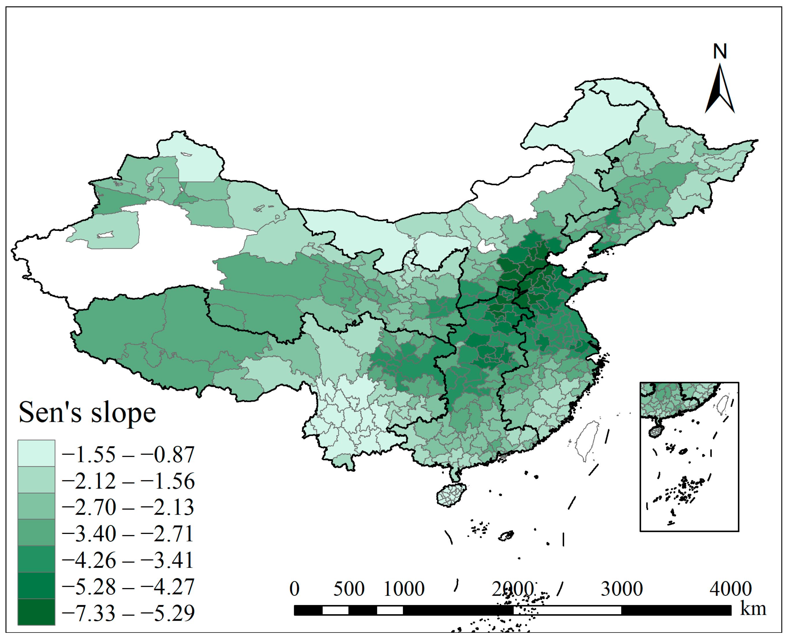
2.3.1. Sen’s Slope Estimation

Sen’s slope estimation is a non-parametric method used to estimate the trend slope of time series data. It is robust and less affected by outliers, making it widely utilized in environmental science, meteorology, and other fields [38]. The method estimates the slope of the best-fit line by calculating the median $S_i$ of the slopes between all pairs of data points. $S_i$ is calculated as follows:

$$S_i={\displaystyle \frac{X_j-X_k}{j-k}}$$

(1)

where j > k, the slope of all time points is calculated, and $X_j$ and $X_k$ are the observed values of PM_2.5 in j and k years. All slopes $S_i$ are sorted, and the median is taken as the Sen’s slope estimation.

2.3.2. Spatial Autocorrelation Analysis

Global spatial autocorrelation was employed to assess the spatial correlation and variability across the entire region, reflecting the degree of autocorrelation of a variable within the study area. This is typically quantified using Moran’s I index. By analyzing Moran’s I index, one can determine the spatial aggregation of the parameter among cities [39,40]. The specific expression of Moran’s I index is

$$I={\displaystyle \frac{n{\sum }_{i=1}^n\sum _{j=1}^n{w}_{ij}\left(x_i-\overline{x}\right)\left(x_j-\overline{x}\right)}{{\sum }_{i=1}^n\sum _{j=1}^n{w}_{ij}{\left(x_i-\overline{x}\right)}^2}}$$

(2)

In the formula, n is the number of cities; $w_{ij}$ is the spatial adjacency matrix; and $x_i$ and $x_j$ represent the pollutant concentration corresponding to different cities, respectively. The value range of Moran’s I index is [−1, 1]. When the value of Moran’s I is greater than 0, it indicates that there is a spatial positive correlation of pollutant concentration, that is, there is a high-high or low-low aggregation of pollutants in adjacent cities. When its value is less than 0, it indicates that there is a spatial negative correlation, that is to say, there is a high–low or low–high discrete distribution of pollutants in adjacent cities; when its value is close to 0, it means that the space is randomly distributed and there is no obvious autocorrelation. This study used the Queen’s case adjacency method to construct the spatial weight matrix. This method defined adjacent cities as 1, and 0 otherwise, which better captured the influence of neighboring cities.

The Z score is used to assess the statistical significance of the Moran’s I index:

$$Z={\displaystyle \frac{I-E\left(I\right)}{\sqrt{Var\left(I\right)}}}$$

(3)

where $E\left(I\right)$ and $Var\left(I\right)$ are the expected value and variance of the Moran’s I, respectively. A Z score greater than 1.96 or less than −1.96 indicates significant spatial autocorrelation at the 95% confidence level, while a Z Score close to 0 suggests no significant autocorrelation.

Local autocorrelation is typically used to assess the aggregation or dispersion of a particular area and its neighboring areas in geographical space, indicating whether there are similar values around a specific geographical unit. In this article, local Moran’s I was used to evaluate the spatial aggregation of local areas. The calculation formula is as follows:

$$I_i={\displaystyle \frac{n\left(x_i-\overline{x}\right)\sum _{j=1}^n{w}_{ij}\left(x_i-\overline{x}\right)}{{\sum }_{i=1}^n{\left(x_i-\overline{x}\right)}^2}}$$

(4)

If the value of I_i is positive, it means that the city i is locally positively correlated with its adjacent cities, showing high–high aggregation or low–low aggregation. The larger the value, the more obvious the spatial correlation; if the value of I_i is negative, the city i is locally negatively correlated with its adjacent cities, showing low–high aggregation or high–low aggregation. A smaller value indicates a larger spatial difference, while a value close to 0 suggests a random spatial distribution with no significant clustering.

2.3.3. GeoDetector

GeoDetector is a spatial statistical method used to explore and detect the spatial distribution of geographic data and its influencing factors [41]. The basic formula is as follows:

$$q=1-{\displaystyle \frac{{\sum }_{h=1}^L{N}_h{\mathsf{\sigma }}_h^2}{N{\mathsf{\sigma }}^2}}$$

(5)

Among them, q represents the explanatory power of the factor to the spatial distribution of variables. The value range is between [0, 1]. The closer it is to 1, the stronger the explanatory power of the factor to the spatial distribution of variables is, whereas the closer it is to 0, the weaker the explanatory power of the factor to the spatial distribution of variables is. L denotes the number of sub-regions in which the study area is divided. N represents the total number of samples in the study area. $N_h$ denotes the number of samples in the h-th subregion. σ² represents the variance of the overall variables in the study area. ${\mathsf{\sigma }}_h^2$ represents the variance of the h-th sub-region variable.

2.3.4. Generalized Additive Model (GAM)

The GAM is a nonparametric regression model that employs a link function on the dependent variable to describe the relationship between the linear predictor and the expected value of the dependent variable. GAM is adept at handling complex data structures by flexibly modeling nonlinear relationships between variables. They offer excellent interpretability and visualization capabilities, making them widely used in data analysis and predictive modeling [27,42]. Its expression is as follows:

$$g\left[E\left(Y\right)\right]={\beta }_0+{\sum }_{j=1}^m{f}_i\left(X_j\right)$$

(6)

where $E\left(Y\right)$ is the expected value of the dependent variable Y, and f_j (X_j) is a smooth function of each independent variable X_j, which can be parametric, such as polynomial or thin-plate regression splines, or non-parametric or semi-parametric and can be estimated using a divergence smoother.

3. Results and Discussion

3.1. Spatio-Temporal Characteristics of PM_2.5

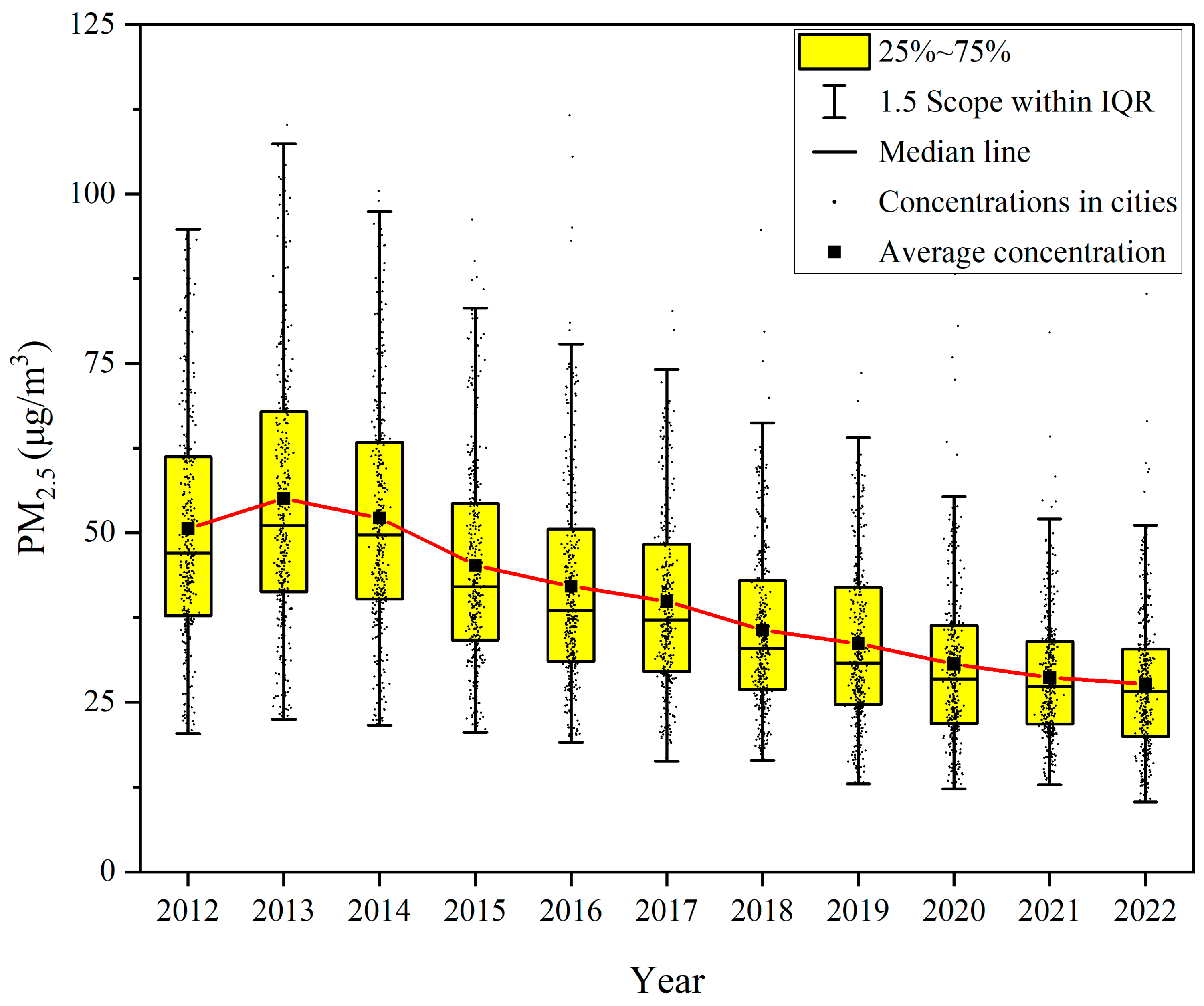
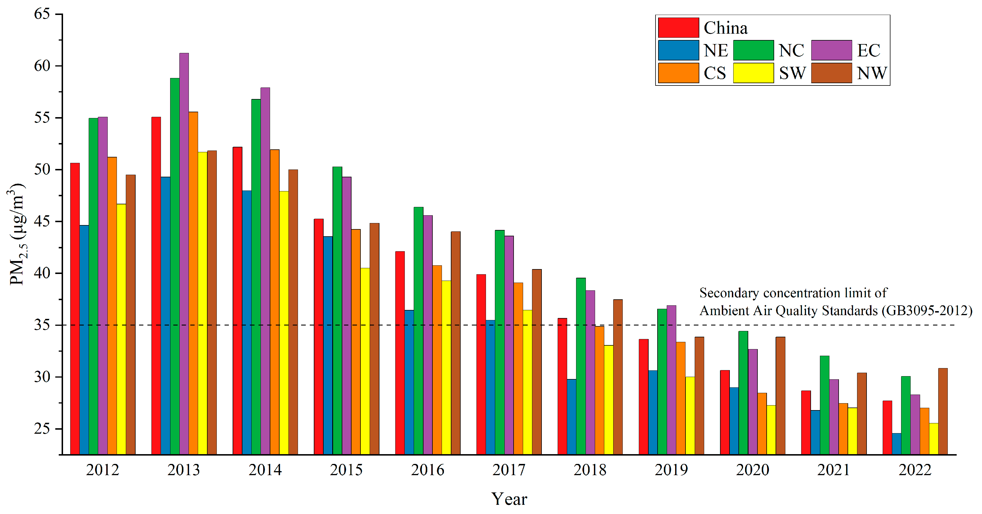
3.1.1. Temporal Variations Characteristics

The trend of the average PM_2.5 concentrations in all cities nationwide is shown in Figure 2. As can be observed, the concentration increased from 50.6 μg/m³ in 2012 to 55.1 μg/m³ in 2013, before decreasing annually from 2013 to 2022. By 2022, the national average PM_2.5 concentration had reduced to 27.7 μg/m³, representing a 49.7% decrease from 2013 levels. Compared with the secondary standard of 35 μg/m³ specified in the “Ambient Air Quality Standards” (GB3095-2012) [43], the national annual average PM_2.5 concentration was below this standard after 2019. However, the national annual concentration remained above the primary standard of 15 μg/m³, throughout the entire study period from 2012 to 2022. The results indicated a marked improvement in PM_2.5 levels since China introduced pollution control policies in 2013.

The changes in the annual average PM_2.5 concentration levels in China and the six major regions from 2012 to 2022 are depicted in Figure 3. Overall, the trends in these six regions were consistent with the national pattern. More specifically, the PM_2.5 concentration levels in north China and east China were consistently higher than the national average. These regions had the highest PM_2.5 levels from 2012 to 2019 and showed the strongest downward trends over the study period. In contrast, the northeast and southwest regions consistently had the lowest concentrations. The northwest region, which was below the national average in 2015 and before, exceeded the national average after 2015 and became the region with the highest concentration in 2022. The concentration in central south China was close to the national average throughout the study period. In general, the national and regional trends in concentrations were more similar to the previously reported results [9,44].

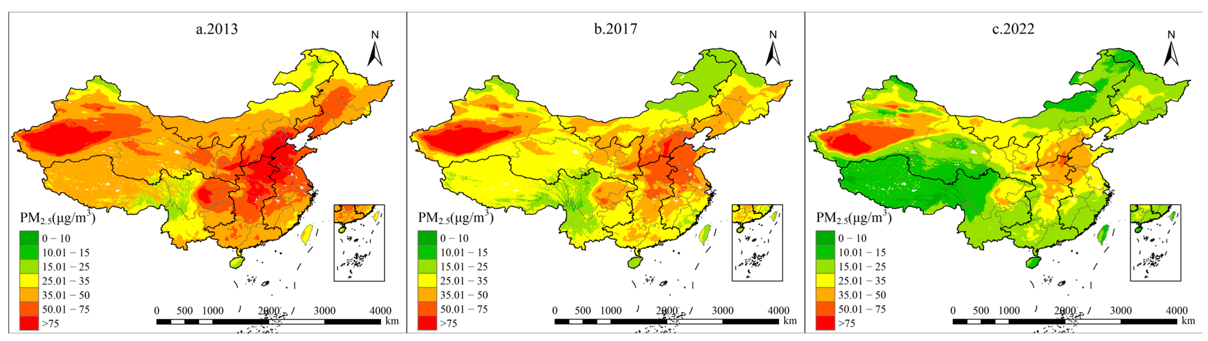
3.1.2. Spatial Distribution Characteristics

To illustrate the differences in the spatial distribution characteristics over time, three representative years were selected: 2013, when the PM_2.5 pollution was most severe; 2017, when the “Blue Sky Protection Campaign” was launched and the first improvements were observed; and 2022, which marked the next stage of air quality management with significant reductions in pollution. These years were used to show the spatial distribution patterns and changes in the PM_2.5 concentration levels nationwide.

As shown in Figure 4, in 2013 (a), the PM_2.5 concentration levels across the country were at high levels. Notably, a large-scale pollution area—designated as the “severe pollution area”—was observed in the southern part of north China, the northern part of central south China, the northern part of east China, and the northeastern part of southwest China. In 2017 (b), a notable decrease in the overall pollution level across the country was detected, accompanied by a reduction in the extent of high-pollution areas. However, the PM_2.5 concentration levels remained high, indicating that pollution was still a serious issue. In 2022 (c), the PM_2.5 pollution had markedly improved nationwide, with the annual average concentration in most areas falling below 35 μg/m³. Although the pollution in the previously high-pollution areas had considerably decreased, these regions remained among the most polluted in the country. Additionally, the Taklimakan Desert and the surrounding areas in southern Xinjiang, while showing some improvement, continued to exhibit high concentration values. Due to the frequent impacts of sandstorms in the region, particulate matter concentrations remained persistently high [45]. Controlling the particulate matter in the “severe pollution area” and desert regions effectively was of great significance for nationwide air pollution prevention and control.

Sen’s slope estimation was utilized to analyze the trend in the PM_2.5 concentration values across China cities from 2012 to 2022. As shown in Figure 5, the Sen’s slope for most cities in China was less than 0, indicating a significant decreasing trend in PM_2.5 concentration levels (p < 0.01). Average annual decreases ranged from 1.48 to 7.33 μg/m³.

Notably, cities within the “severe pollution area”, such as Beijing, Tianjin, and provinces like Henan, Hebei, and Shandong, experienced the most substantial decreases in the PM_2.5 concentration levels. This outcome indicated significant improvements in the air quality in these regions, reflecting effective air pollution control measures. On the contrary, relatively smaller decreases were observed in the coastal areas of south China, Inner Mongolia, and Heilongjiang, where initial pollution levels were low.

The analysis showed that PM_2.5 pollution levels significantly decreased in key regions of China following the implementation of various control policies. The results of the spatio-temporal variation characteristics indicated that China’s pollution control policies have been successful in improving air quality, enhancing public health, and fostering more resilient economic development.

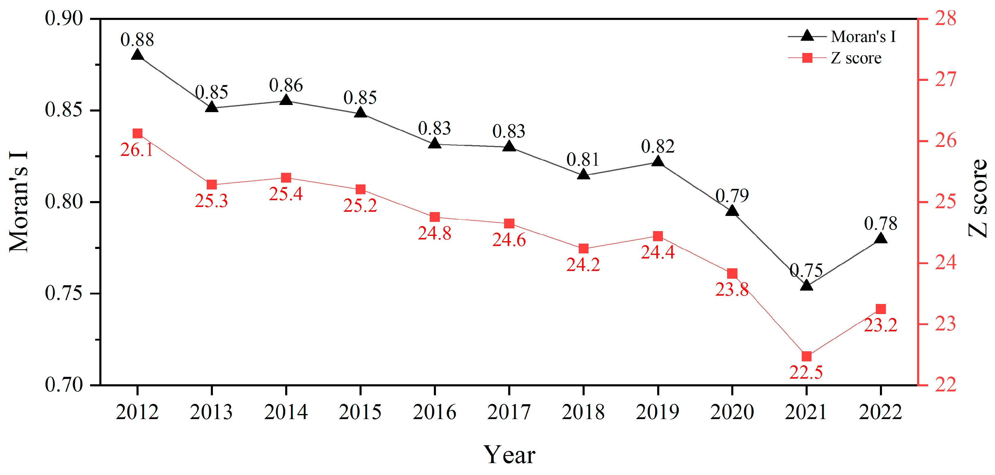
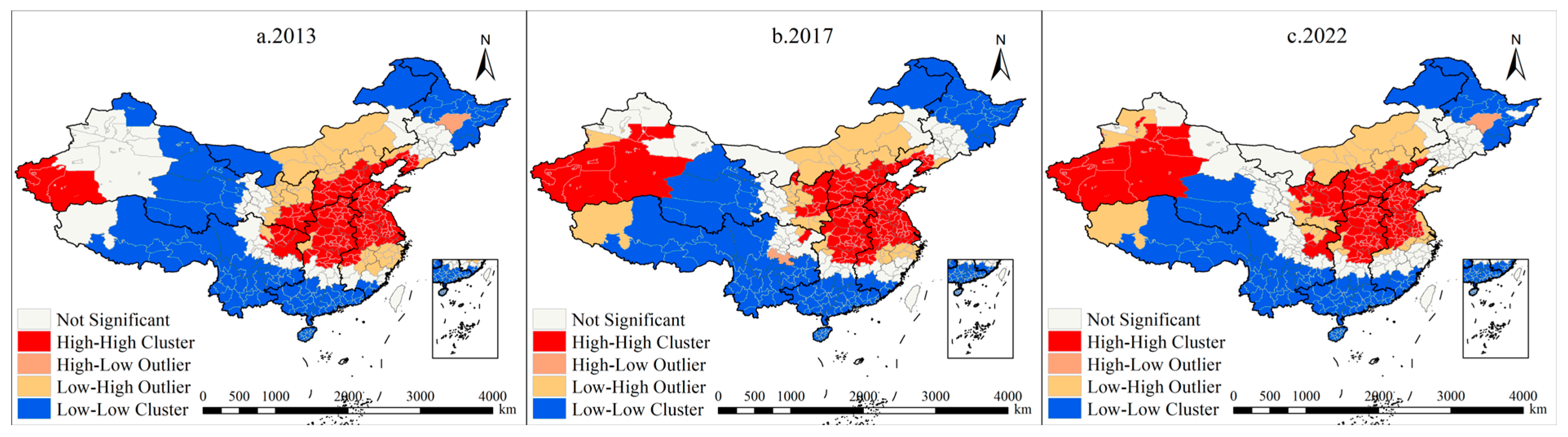
3.2. Spatial Clustering Characteristics

To study the aggregation of the spatial distribution of PM_2.5 in China from 2012 to 2022, the global Moran’s I for each year is presented in Figure 6. The higher the Moran’s I, the stronger the correlation of PM_2.5 concentrations between adjacent cities; conversely, the lower the Moran’s I, the weaker the correlation. The index revealed significant spatial autocorrelation each year (p < 0.01), indicating a clear spatial clustering of the PM_2.5 concentration levels among cities in China. This result suggested that the PM_2.5 levels in a city were affected not only by its conditions but also by those in neighboring cities. The Moran’s I index ranged from 0.75 to 0.88, and the Z score varied between 22.5 and 26.1. This clustering suggested that the pollution levels in cities not only were determined by local factors but were also influenced by neighboring cities, highlighting the interconnected nature of environmental challenges across regions. Throughout the study period, these values generally showed a declining trend, reflecting that while the PM_2.5 concentration levels in China consistently exhibited spatial clustering, this effect gradually diminished. This reduction in spatial correlation indicated the success of pollution control measures that have contributed to breaking down regional pollution concentrations, signaling progress toward more balanced, sustainable urban development. Compared with studies at smaller regional scales, PM_2.5 across all cities in China exhibited stronger spatial autocorrelation [46].

By applying the local autocorrelation method, we generated maps depicting the spatial aggregation of PM_2.5 concentrations in Figure 7 for 2013 (a), 2017 (b), and 2022 (c) to highlight their local correlation patterns. The findings showed similar aggregation trends throughout these years. The distribution of the high–high concentration areas remained largely unchanged, primarily centered in the “severe pollution area”. These regions continued to form extensive high–high concentration zones, indicating significant spatial clustering of elevated PM_2.5 levels. This clustering was predominantly due to the development of heavy industry and widespread coal usage in these areas. In southern Xinjiang, the presence of the Taklimakan Desert, coupled with unique natural conditions, such as aridity and basin terrain, contributed to the accumulation of PM_2.5, resulting in consistently high particulate matter concentrations in this region [47]. In parallel, an obvious high–high clustering distribution was also recorded. These high PM_2.5 concentration areas are particularly important for targeted policy intervention as they represent the regions with the most severe air quality challenges and where pollution control measures are most needed. There were generally no obvious high–low clustering areas across the country.

The distribution of the low–high accumulation areas was generally consistent with the main clusters found in the Inner Mongolia Autonomous Region and the coastal areas of east China adjacent to high–high accumulation areas. On the contrary, the range of the low–low agglomeration areas gradually shrank and was mainly distributed in the southwest, the coastal areas of the central and southern regions, and parts of the northwest and northeast regions. These areas were less affected by heavy industry. In addition, the favorable meteorological conditions promoted the spread and settling of particulate matter, leading to lower PM_2.5 concentrations.

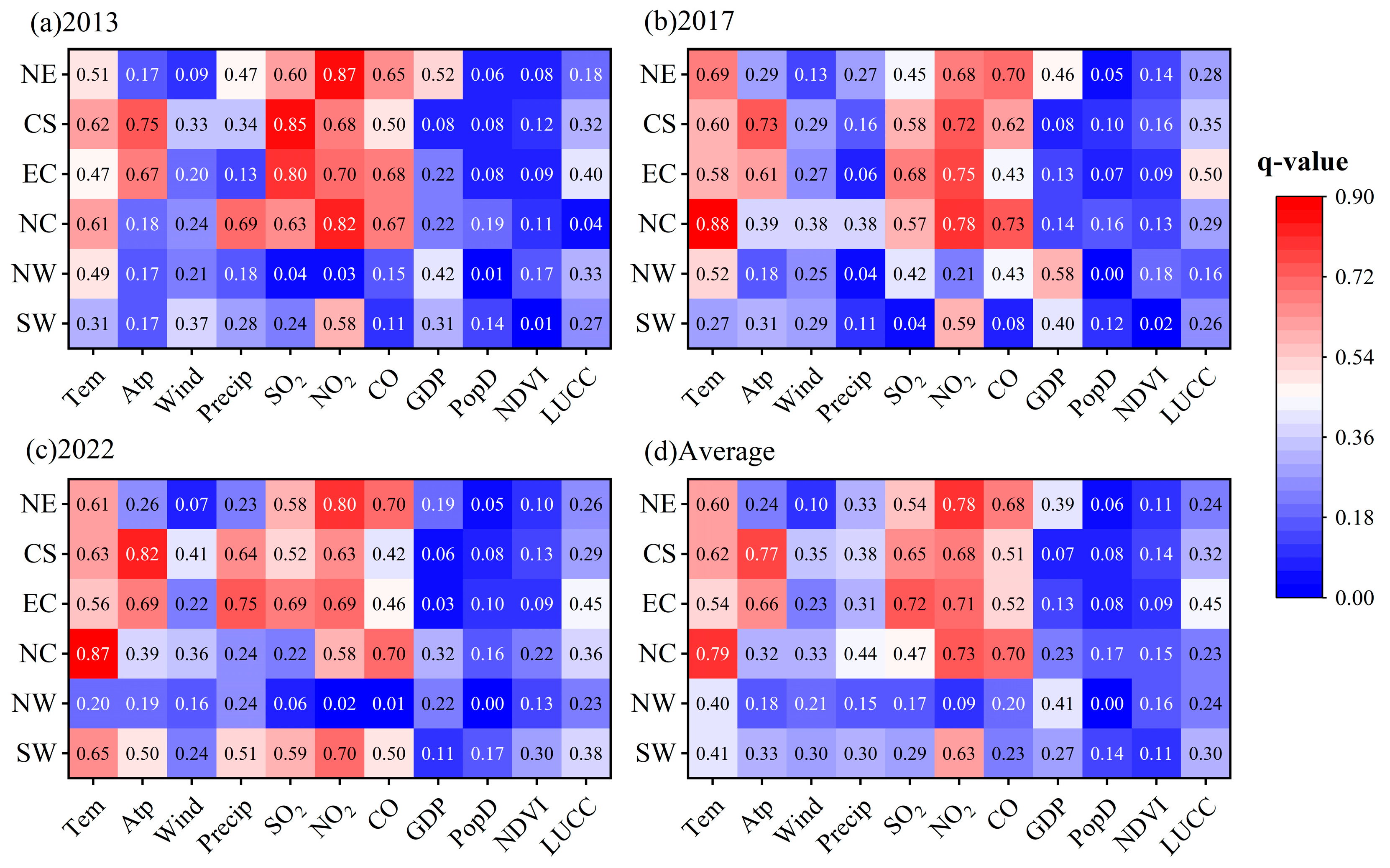
3.3. Detection of Six Regional Impact Factors

This study used the GeoDetector method to assess the impacts of various factors on PM_2.5 concentrations across six regions of China (northeast, north, east, central south, northwest, and southwest) during three representative years: 2013, 2017, and 2022. The analysis was based on the q-value, which reflected the explanatory strength of PM_2.5 by factors such as the temperature, atmospheric pressure, wind speed, precipitation, SO₂, NO₂, CO, population density, NDVI, and LUCC. The GDP was evaluated at the city scale, while other factors were analyzed using grid points sampled at equal distances across the study area. The number of grid points varied by region, ranging from 2204 in east China to 9233 in northwest China.

Using the GeoDetector, the q-values for the six regions for 2013, 2017, and 2022 and the averages of these three years were obtained, as shown in Figure 8. A higher q value suggested a stronger influence of the factor on the spatial variation of the target variable. The analysis revealed substantial regional variation in the driving factors influencing PM_2.5 concentrations, with distinct temporal trends across different areas.

The results of Figure 8 revealed significant regional variations and temporal trends in the driving factors of the PM_2.5 concentration levels, highlighting both the complexity of pollution mechanisms and the distinct characteristics of each region. Overall, pollutant concentrations, particularly NO₂, SO₂, and CO, were identified as dominant drivers of the spatial distribution of PM_2.5 across most regions, underscoring the influence of industrial emissions, coal combustion, and vehicular exhaust. Similar to most research findings, NO₂, SO₂, and CO all showed significant impacts on PM_2.5 concentrations [48]. For example, the NO₂ and CO concentrations remained the primary factors affecting the PM_2.5 distribution in northeast China, reflecting the region’s dependence on industrial activities and transportation emissions. In contrast, regions such as central south and east China were more strongly affected by meteorological factors like atmospheric pressure, which played a critical role in atmospheric circulation and the accumulation or dispersion of pollutants [49,50]. These regions were often affected by unstable atmospheric pressure systems due to their geographical location, influencing the PM_2.5 concentrations. Some studies on these two regions have also shown the significant impacts of meteorological factors on PM_2.5 concentrations [51].

Next, we conducted an analysis of the results for different regions. The results for northeast China demonstrated that NO₂ consistently exhibited the highest q-values in terms of spatial impact, with CO and SO₂ also significantly contributing to the spatial distribution of PM_2.5 concentrations, particularly in 2013 and 2017. However, the spatial influence of SO₂ began to diminish by 2022, likely due to the implementation of stricter controls on coal burning and industrial emissions in recent years. Similarly, in north China, the NO₂ and CO concentrations were the key drivers of the spatial distribution of PM_2.5 concentrations, although their impact began to decrease following the Air Pollution Prevention and Control Action Plan. In both regions, temperature and precipitation also played a notable role in affecting the spatial patterns of pollution, further illustrating the complex interplay between meteorological factors and anthropogenic emissions.

In central south China, atmospheric pressure was identified as the most significant factor across all three years, with a consistently high q-value. The difference in the atmospheric pressure between the inland and coastal areas of the region, coupled with the influence of atmospheric circulation patterns, significantly affected the accumulation of PM_2.5. In east China, there was a clear north–south difference across the region as Shandong and Jiangsu in east China are heavily affected by industry and agriculture. Therefore, the NO₂ and SO₂ emissions from industrial and agricultural activities have also become the most important factors, in terms of affecting the PM_2.5 concentration levels.

The northwest region showed a distinct pattern. Economic activity, measured by GDP, was the main driver of PM_2.5 levels. This suggested that economic development in cities like Xi’an and the Tianshan urban agglomeration contributed to rising pollution. Pollutants had a relatively smaller impact compared with other regions, suggesting that the PM_2.5 concentration levels in northwest China may be more closely related to factors such as urban expansion and economic growth, rather than industrial emissions alone.

In southwest China, the Chengdu–Chongqing region, located in the Sichuan Basin, exhibited high q-values for the NO₂ concentration, showing the contribution of NO₂ concentration to the spatial differentiation of PM_2.5 concentration in the region. In addition, the basin’s unique topography exacerbated the accumulation of pollutants, making meteorological conditions an important driver [52,53].

It was further highlighted that while meteorological factors—such as wind speed, temperature, and precipitation—influenced PM_2.5 concentrations to varying degrees across different regions, their role remained significant, especially in areas like central south and east China. These regions were more susceptible to atmospheric circulation patterns, which contributed to the accumulation of PM_2.5. Conversely, factors such as population density, NDVI, and land use/land cover change (LUCC) had a relatively low impact on the PM_2.5 concentration levels in most regions, although population density had a more pronounced effect in north and southwest China, where industrial activities and road traffic emissions were closely associated with high population densities. The latter occurred particularly in polluted regions like the Beijing–Tianjin–Hebei area and the Sichuan Basin. These findings highlighted how environmental, meteorological, and socio-economic factors interacted to shape PM_2.5 concentrations, providing critical insights for developing more sustainable air quality management strategies. In addition, these findings highlighted the importance of targeted policy interventions to address regional disparities. By tailoring interventions to regional characteristics, we can promote environmental equity and sustainable development across different regions, ultimately contributing to healthier cities and more balanced urban growth.

3.4. The Influence Mechanism of Driving Factors

3.4.1. Nonlinear Response Mechanism of Driving Factors

To explore the specific response mechanisms and regional differentiation of various driving factors on PM_2.5 concentration levels, we used the GAM to observe the variations in PM_2.5 concentrations under specific meteorological, social development, and other conditions, thereby providing recommendations for pollution forecasting and urban development planning. The spatial distribution maps for each driving factor in 2022 are shown in Figure S3. Meteorological, economic, pollutant, and other factors exhibited distinct spatial aggregation characteristics. For example, the areas with high temperature values were mainly in southern China and southern Xinjiang. In contrast, high concentrations of NO₂ were predominantly found in north China, especially in the Beijing–Tianjin–Hebei region and its surrounding areas. Conversely, NDVI increased from west to east, reflecting noticeable spatial variation.

To perform the GAM analysis, logarithmic transformation was applied to the GDP and population density data to account for their actual distributions, while other data were used in their original form for model testing.

Table 1. Estimation results in GAM.

Factors	edf	F	p-Value
s(Temperature)	6.45	36.37	<2 × 10−16 ***
s(Atmospheric Pressure)	8.411	27.26	<2 × 10−16 ***
s(Precipitation)	8.114	21.64	<2 × 10−16 ***
s(Wind Speed)	5.481	10.94	<2 × 10−16 ***
s(SO2)	7.383	12.96	<2 × 10−16 ***
s(NO2)	2.846	66.7	<2 × 10−16 ***
s(CO)	1.69	91.01	<2 × 10−16 ***
s(Log_GDP)	3.312	5.23	0.000356 ***
s(Log_PopDensity)	6.762	9.845	<2 × 10−16 ***
s(NDVI)	7.014	7.654	<2 × 10−16 ***

Note: ***: p < 0.01.

presents the results of the GAM analysis. All factors were found to be statistically significant (p < 0.01), confirming their relevance in the analysis. In the result, the edf (effective degrees of freedom) indicated the flexibility of the smooth term, and F assessed the significance of the smooth term’s contribution to the model.

The results showed that all driving factors exhibited non-linear responses. Among them, CO and NO₂ exhibited the highest F values, suggesting they had the greatest impact on the PM_2.5 concentration levels. This was followed by temperature and atmospheric pressure, which also played significant roles but to a lesser extent.

The response of the PM_2.5 concentration to temperature initially increased and then decreased, peaking around 15 °C [Figure 9a]. The temperature distribution map in Figure S3a showed that colder regions were primarily located in Tibet, Qinghai, and the Greater Khingan Mountains in the northeast. In these regions, the low intensity of human activities and the high vegetation coverage in the Greater Khingan Mountains contributed to lower PM_2.5 concentration levels [54]. Areas with temperatures around 14 °C predominantly included the “highly polluted areas” in north China, where industrial development, coal burning, and other wintertime human activities significantly contributed to higher PM_2.5 concentration levels. Conversely, regions with average annual temperatures above 17 °C, such as the southern part of south-central China and the southeastern coastal areas of east China, experienced higher temperatures throughout the year. This increased temperature promoted air convection, which enhanced the dispersion of particulate matter and affected the PM_2.5 concentration levels [55,56]. Additionally, there was minimal coal burning in these areas during winter, leading to a significant decrease in the PM_2.5 concentration levels as the temperature rose.

For atmospheric pressure (Figure 9b), as the atmospheric pressure rose, PM2.5 concentrations showed a fluctuating upward trend. This was primarily because high atmospheric pressure led to atmospheric subsidence, which inhibited vertical convection and caused PM_2.5 to accumulate locally. In contrast, low atmospheric pressure enhanced the upward movement of the atmosphere, facilitating the vertical diffusion of pollutants [55] and thereby reducing the PM_2.5 concentration levels.

For wind speed [Figure 9c], when wind speeds ranged from 0 to 2.5 m/s, the PM_2.5 concentration levels increased with wind speed. At low and relatively stable wind speeds, the atmosphere’s vertical and horizontal diffusion capabilities were weak, leading to the accumulation of particulate matter. As the wind speed increased, the concentration of PM_2.5 rapidly decreased. This effect was due to the enhanced diffusion and dilution effects of higher wind speeds on the atmosphere; stronger winds more effectively dispersed and diluted PM_2.5, reducing its concentration [27,57].

For precipitation [Figure 9d], the overall trend showed a decrease in the PM_2.5 concentration levels. This reduction was primarily due to the scouring effect of precipitation, which helped remove particulate matter from the air. At low levels of precipitation, the decrease in PM_2.5 was more pronounced. However, as precipitation increased, the decline in the PM_2.5 concentration levels became more gradual. There was a noticeable rebound in the PM_2.5 concentration levels when precipitation ranged between 0.3 and 0.5 mm. The reason for this rebound was that at low levels of rainfall, the growth of aerosols through moisture and the conversion of gases to particles increased the concentration of aerosols. Conversely, higher levels of precipitation were more effective at removing these aerosol particles from the atmosphere, leading to a reduction in the PM_2.5 mass concentration levels [58].

For SO₂ (Figure 9e), NO₂ (Figure 9f), and CO concentrations (Figure 9g), PM_2.5 continued to increase as the concentrations of these three pollutants increased. However, when the SO₂ concentration was high, a decrease in the fluctuation occurred. SO₂ and NO₂ were recognized as crucial precursors in the formation of secondary particulate matter. Thus, high concentrations of SO₂ and NO₂ were closely associated with high concentrations of PM_2.5. Additionally, CO played an indirect role in influencing PM_2.5 concentrations in atmospheric chemical processes, contributing to the formation of secondary particulate matter [59]. Under the influence of the chemical reactions, the PM_2.5 concentrations also increased accordingly in areas with high CO concentrations [60]. Taking into account that the primary sources of SO₂ included fossil fuel combustion, smelting, chemical production, and transportation, its regional distribution exhibited distinct geographical characteristics (Figure S3e). The development of coal mining and smelting industries in some areas has resulted in some of the highest regional SO₂ concentrations in the country, such as Shizuishan in Ningxia, Wuhai City in Inner Mongolia, Datong in Shanxi, and their neighboring areas. However, these areas had fewer other sources of emissions, so the PM_2.5 concentration levels were not unduly elevated. Despite this effect, other emission sources in these regions were relatively minimal, preventing excessive rises in the PM_2.5 levels. Conversely, NO₂ and CO primarily reflected industrial emissions and motor vehicle exhaust, suggesting that without proper control of these emissions, the PM_2.5 concentration levels would continue to rise. As illustrated in Figure S3f,g, the regions with the highest NO₂ and CO concentrations closely aligned with the “severe pollution area” exhibiting the highest PM_2.5 concentration levels, thereby highlighting the principal contributors to PM_2.5 pollution.

For GDP (Figure 9h), the relationship exhibited an inverted “U”-shaped curve. More specifically, the PM_2.5 concentration levels initially increased with rising urban GDP, before decreasing as the GDP continued to grow. The peak occurred around CNY 36,000. It showed a similar trend to the peak of CNY 39,471 observed in the previous study by Zhao et al. [61]. This pattern aligned with the environmental Kuznets curve, which posited that environmental degradation initially increased with economic development but eventually declined as a country became more affluent and adopted cleaner technologies [62]. This trend suggested that during the early phases of economic growth, factors like increased fossil fuel use, industrial expansion, infrastructure growth, and the rise in motor vehicle numbers were key contributors to elevated PM2.5 concentrations. The rapid industrialization and urbanization processes led to elevated vehicle exhaust emissions and consequently increased PM_2.5 levels. As economic development progressed and reached a certain threshold, the industrial structure typically transformed. Subsequently, more stringent policies and regulations, enhanced pollution source supervision, and the promotion of clean energy contributed to a reduction in the PM_2.5 concentration levels.

Similarly, the pattern observed for the population density (Figure 9i) paralleled that of the GDP. Higher population density was often associated with more advanced economic development, which in turn influenced the PM_2.5 concentration levels. Consequently, the effect of population density on PM_2.5 concentrations mirrored the trend seen with changes in the total economic volume. The process of urbanization in China had a complex impact on PM_2.5 concentrations [63].

As far as NDVI is concerned (Figure 9j), as it increased, the concentration of PM_2.5 consistently decreased. This was primarily attributed to the strong adsorption and sedimentation effects of vegetation on particulate matter, which resulted in reduced PM_2.5 concentration levels as NDVI values rose [64,65]. A minor rebound was observed at an NDVI value of 0.75. As indicated in Figure S3i, this range corresponded to the NDVI values in China’s highly polluted areas. In these regions, social development factors may dominate, leading to an increase in the PM_2.5 concentration levels within this interval.

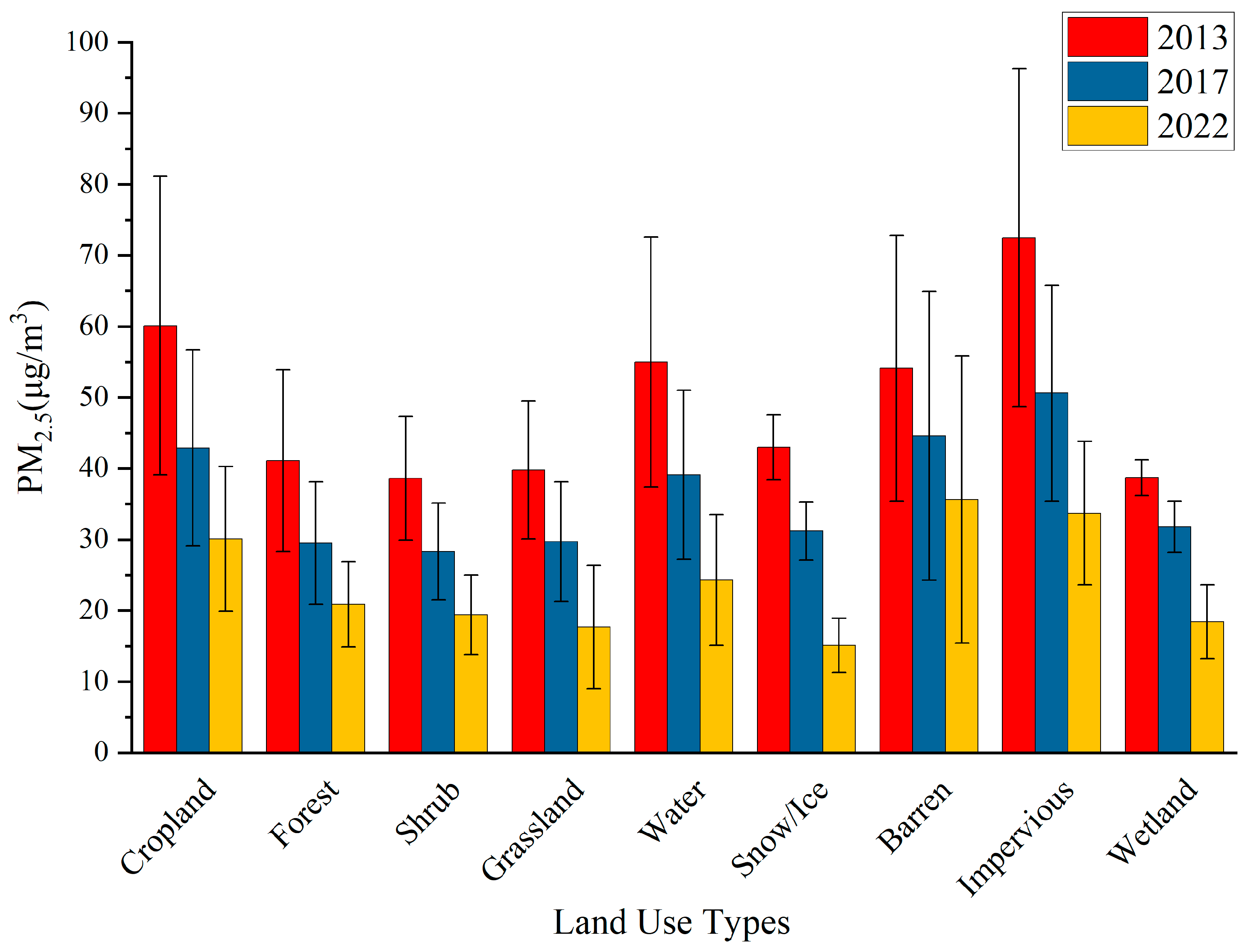
3.4.2. The Influence Mechanism of Land Use Types

We combined the spatial distribution characteristics of land use types in 2013, 2017, and 2022 (Figure S4) and compared the differences and changes in the PM_2.5 concentrations under nine land use types. Understanding the role of land use in air quality management is crucial for promoting sustainable urban development and improving environmental health. The overall distribution of land use types across the three years remained relatively consistent. The barren type was predominantly located in much of the northwest region, and cropland was mainly found in southern north China, northern northeastern China, northern central and southern China, and western northeastern China. The forest type was distributed across most of southern China, and grassland occupied most of the western region, excluding areas classified as barren. Impervious surfaces were concentrated in areas with higher population density. Additionally, specialized land use types, such as shrub, water, snow/ice, and wetland, were scattered throughout various regions of China.

According to the comparison of the PM_2.5 concentration changes across nine different land use types (Figure 10), it was evident that the average PM_2.5 concentration for each land use type had significantly decreased. Among the three selected years, cropland, barren, and impervious areas consistently exhibited higher PM_2.5 concentration levels compared with the national average. The PM_2.5 concentration levels in the water area were higher than the national average in 2013 and 2017 but lower in 2022. In contrast, the remaining five land use types—forest, shrub, grassland, snow/ice, and wetland—had PM_2.5 concentrations consistently below the national average across all three years. An analysis of the standard deviation revealed substantial variability in the PM_2.5 concentration levels for cropland, barren, impervious, and water, while the concentrations for forest, shrub, grassland, snow/ice, and wetland remained relatively stable. From 2013 to 2022, the variability in the PM_2.5 concentration levels for cropland, impervious, and water was decreased, whereas barren continued to exhibit significant variability. Accordingly, we need to focus on the role of land management and urban planning in improving air quality and reducing pollution.

Specifically, in 2013, impervious surfaces exhibited the highest average PM_2.5 concentration, significantly surpassing other land use types. This distribution was closely aligned with areas of high population density, indicating that regions with extensive impervious surfaces—such as buildings, roads, and other hardened surfaces—were heavily populated. The prevalence of these surfaces in densely populated areas reflected substantial human activity. In 2013, a period of rapid development in China, the extensive use of impervious surfaces for construction and infrastructure correlated with elevated industrial pollutant emissions and increased motor vehicle exhaust. This could explain the notably high PM_2.5 concentrations associated with impervious areas during that time [66,67]. Following impervious surfaces, cropland and water also exhibited notable PM_2.5 concentration levels. In cropland areas, various agricultural activities, such as mechanical farming, irrigation, and pesticide application, significantly contributed to the PM_2.5 levels. These practices generated dust and particulate matter, while biomass burning further exacerbated PM_2.5 concentration levels in agricultural regions [67]. Water bodies, primarily used for shipping, also contributed to the PM_2.5 concentrations. Industrial emissions from regions along major waterways, such as the Yangtze River Economic Belt, exacerbated pollution levels. Additionally, emissions from shipping activities significantly impacted PM_2.5 concentrations [68].

In 2017, the impervious type continued to exhibit the highest PM_2.5 concentration, although the disparity with other land use types diminished. The PM_2.5 concentration in cropland also saw a significant reduction, primarily due to stringent regulations on straw burning, which effectively curtailed the PM_2.5 emissions from agricultural activities. Similarly, the concentration of PM_2.5 in water bodies markedly decreased, reflecting China’s enhanced control over industrial emissions.

In 2022, the PM_2.5 concentration levels in impervious land areas significantly declined. In addition, the barren type surpassed the impervious type to record the highest PM_2.5 concentration levels among all land use types. The elevated PM_2.5 levels in barren areas were primarily attributed to the absence of vegetation cover, making these regions highly susceptible to wind erosion and prone to sandstorms, which generated large quantities of dust and particulate matter [47]. In addition, the higher surface temperature of barren land further facilitated the resuspension of particulate matter, exacerbating the PM_2.5 concentration levels in these areas [69].

The PM_2.5 concentrations of the other land use types had always remained at low levels in these three years. The main reason was that under land use types, such as forest, shrub, grassland, and wetland, vegetation grew well, helping to absorb airborne particles and reduce their resuspension, leading to lower PM_2.5 concentrations [70,71]. Snow/ice can also capture and adsorb particles in the air, and snow can also remove atmospheric particles. Therefore, the PM_2.5 concentration levels were usually lower in snow/ice areas [72]. For Snow/Ice, there had been a more obvious concentration decrease. This may be due to the global warming effect. The melting of Snow/Ice, mainly in parts of the Tibetan Plateau, had enhanced the wet deposition of PM_2.5, which was enhanced by the temperature rise. As a result, the atmospheric convection was reduced and the reduction in the PM_2.5 concentration levels was promoted [73]. In addition, it was also related to the significant reduction in the overall concentration level in the northwest region due to the improvement of pollution conditions in the Sichuan Basin.

4. Conclusions

In this work, we analyzed the spatial and temporal variations of the PM_2.5 concentration levels in China from 2012 to 2022. In addition, we investigated the main driving factors of the PM_2.5 concentration changes and their complex nonlinear response mechanisms. The results showed that the PM_2.5 concentration levels in China peaked in 2013 and then continued to decline. The pollution levels remained high in the northern and eastern regions. The main pollution clusters were located in the North China Plain, the Middle and Lower Yangtze River Plain, and the Sichuan Basin. However, all of these regions showed significant decreases in the PM_2.5 concentration levels. Through the combined analysis of the GeoDetector and GAM, we found significant regional differentiation in various driving factors. Additionally, there was a complex nonlinear relationship between PM_2.5 and the various driving factors. The conclusions were as follows: (1) Meteorological factors affected PM_2.5 through diffusion, dilution, and deposition with significant regional differences. (2) Regions with high concentrations of SO₂, NO₂, and CO were typically associated with high concentrations of PM_2.5. However, in coal-rich regions, sustained elevation of sulfur dioxide may reduce PM_2.5 due to specific geographic and industrial conditions. (3) GDP and population density showed an inverted “U” shape with the PM_2.5 relationship, reflecting the environmental Kuznets curve, where pollution rose in the early stages of development but fell with stricter controls after a certain threshold was reached. (4) A higher NDVI led to lower PM_2.5 due to the adsorption and deposition effects of vegetation. Finally, we studied the impacts of land use types on PM_2.5 concentrations. There were significant differences in the PM_2.5 concentration levels by land use type, with higher concentrations primarily under the cropland, barren, and impervious types.

In conclusion, the findings emphasized the importance of region-specific strategies for air quality management. Sustainable development should be at the core of future air quality management policies. Future policies should be tailored to the specific characteristics and dominant drivers of each region. The main policy recommendations are as follows: (1) Based on the impact and prediction of meteorological factors on PM_2.5, it is essential to establish and improve meteorological monitoring networks to promptly issue early warning information on PM_2.5 concentrations, providing decision-making support for the public and relevant authorities. (2) Relevant departments should strengthen the management of coal burning and industrial emissions and control the release of SO₂, NO₂, and CO. Encouraging the adoption of cleaner, greener technologies in industries can significantly reduce emissions, contributing to both economic and environmental sustainability. (3) The results of spatial autocorrelation indicated a strong spatial correlation of PM_2.5 concentrations between Chinese cities; thus, it is important to pay attention to intercity joint prevention and control and strengthen regional cooperative governance. (4) The influence of GDP and population density on PM_2.5 followed the environmental Kuznets curve. Policies should promote the transition to a green economy, strengthen environmental regulations, and encourage technological innovation to effectively reduce PM_2.5 pollution while ensuring economic growth. (5) PM_2.5 concentrations showed significant differences under different land use types and NDVI. Therefore, promoting green urban planning and restoring natural ecosystems are key steps in ensuring a sustainable urban environment and reducing pollution.

Although this work has made significant progress in revealing the spatio-temporal evolution of the PM_2.5 concentration levels in China and their driving mechanisms, there are still some limitations. For example, the study was based on annual average data and did not delve into the seasonal and daily variations of PM_2.5, overlooking the dynamic impacts of pollution sources and meteorological factors at different times of the year. Future works could refine the time scale by exploring seasonal fluctuations and diurnal variations in PM_2.5. In addition, the factors we selected are still insufficient. For example, air pollution transported by wind has a significant impact on some cities. And low-atmosphere evolution and some synoptic patterns may affect PM_2.5 pollution. These factors need to be given special consideration in future research.

References

1. Li, C. Reversal of trends in global fine particulate matter air pollution. Nat. Commun. 2023, 14, 5349. [Google Scholar] [CrossRef]
2. Li, Z.; Liu, Q.; Chen, L.; Zhou, L.; Qi, W.; Wang, C.; Zhang, Y.; Tao, B.; Zhu, L.; Martinez, L.; et al. Ambient air pollution contributed to pulmonary tuberculosis in China. Emerg. Microbes Infect. 2024, 13, 2399275. [Google Scholar] [CrossRef]
3. Hoek, G.; Krishnan, R.M.; Beelen, R.; Peters, A.; Ostro, B.; Brunekreef, B.; Kaufman, J.D. Long-term air pollution exposure and cardio-respiratory mortality: A review. Environ. Health 2013, 12, 43. [Google Scholar] [CrossRef] [PubMed]
4. Guo, C. Effect of long-term exposure to fine particulate matter on lung function decline and risk of chronic obstructive pulmonary disease in Taiwan: A longitudinal, cohort study. Lancet Planet. Health 2018, 2, e114–e125. [Google Scholar] [CrossRef]
5. Yao, P.-T.; Peng, X.; Cao, L.-M.; Zeng, L.-W.; Feng, N.; He, L.-Y.; Huang, X.-F. Evaluation of a new real-time source apportionment system of PM2.5 and its implication on rapid aging of vehicle exhaust. Sci. Total Environ. 2024, 937, 173449. [Google Scholar] [CrossRef] [PubMed]
6. Liu, H. The impacts of regional transport on anthropogenic source contributions of PM2.5 in a basin city, China. Sci. Total Environ. 2024, 917, 170038. [Google Scholar] [CrossRef] [PubMed]
7. Yang, H.; Yao, R.; Sun, P.; Ge, C.; Ma, Z.; Bian, Y.; Liu, R. Spatiotemporal Evolution and Driving Forces of PM2.5 in Urban Agglomerations in China. Int. J. Environ. Res. Public Health 2023, 20, 2316. [Google Scholar] [CrossRef]
8. She, Y.; Chen, Q.; Ye, S.; Wang, P.; Wu, B.; Zhang, S. Spatial-temporal heterogeneity and driving factors of PM2.5 in China: A natural and socioeconomic perspective. Front. Public Health 2022, 10, 10. [Google Scholar] [CrossRef]
9. Liu, B.; Wang, L.; Zhang, L.; Bai, K.; Chen, X.; Zhao, G.; Yin, H.; Chen, N.; Li, R.; Xin, J.; et al. Evaluating urban and nonurban PM2.5 variability under clean air actions in China during 2010–2022 based on a new high-quality dataset. Int. J. Digit. Earth 2024, 17, 2310734. [Google Scholar] [CrossRef]
10. Huang, H.; Jiang, P.; Chen, Y. Analysis of the Social and Economic Factors Influencing PM2.5 Emissions at the City Level in China. Sustainability 2023, 15, 16335. [Google Scholar] [CrossRef]
11. Wang, Y.; Gao, W.; Wang, S.; Song, T.; Gong, Z.; Ji, D.; Wang, L.; Liu, Z.; Tang, G.; Huo, Y.; et al. Contrasting trends of PM2.5 and surface-ozone concentrations in China from 2013 to 2017. Natl. Sci. Rev. 2020, 7, 1331–1339. [Google Scholar] [CrossRef]
12. He, K.; Huo, H.; Zhang, Q. Urban Air Pollution in China: Current Status, Characteristics, and Progress. Annu. Rev. Environ. Resour. 2002, 27, 397–431. [Google Scholar] [CrossRef]
13. Chen, C.; Gao, B.; Xu, M.; Liu, S.; Zhu, D.; Yang, J.; Chen, Z. The spatiotemporal variation of PM2.5-O3 association and its influencing factors across China: Dynamic Simil-Hu lines. Sci. Total Environ. 2023, 880, 163346. [Google Scholar] [CrossRef]
14. He, J.; Ding, S.; Liu, D. Exploring the spatiotemporal pattern of PM2.5 distribution and its determinants in Chinese cities based on a multilevel analysis approach. Sci. Total Environ. 2019, 659, 1513–1525. [Google Scholar] [CrossRef]
15. Xu, W.; Wang, Y.; Sun, S.; Yao, L.; Li, T.; Fu, X. Spatiotemporal heterogeneity of PM2.5 and its driving difference comparison associated with urbanization in China’s multiple urban agglomerations. Environ. Sci. Pollut. Res. 2022, 29, 29689–29703. [Google Scholar] [CrossRef]
16. Hu, J.; Wang, Y.; Ying, Q.; Zhang, H. Spatial and temporal variability of PM2.5 and PM10 over the North China Plain and the Yangtze River Delta, China. Atmos. Environ. 2014, 95, 598–609. [Google Scholar] [CrossRef]
17. Wu, Q.; Guo, R.; Luo, J.; Chen, C. Spatiotemporal evolution and the driving factors of PM2.5 in Chinese urban agglomerations between 2000 and 2017. Ecol. Indic. 2021, 125, 107491. [Google Scholar] [CrossRef]
18. Wang, J.; Li, R.; Xue, K.; Fang, C. Analysis of Spatio-Temporal Heterogeneity and Socioeconomic driving Factors of PM2.5 in Beijing–Tianjin–Hebei and Its Surrounding Areas. Atmosphere 2021, 12, 1324. [Google Scholar] [CrossRef]
19. Xue, L.; Xue, C.; Chen, X.; Guo, X. Spatial–temporal evolution characteristics of PM2.5 and its driving mechanism: Spatially explicit insights from Shanxi Province, China. Environ. Monit. Assess. 2024, 196, 632. [Google Scholar] [CrossRef] [PubMed]
20. Tang, D.; Lu, Y.; Cai, W.; Zhu, X. Temporal and Spatial Distribution Characteristics of Air Pollution and the influence of Energy Structure in Guangdong-Hong Kong-Macao Greater Bay Area. IOP Conf. Ser. Earth Environ. Sci. 2020, 446, 032029. [Google Scholar] [CrossRef]
21. Wang, H.; Zhang, M.; Niu, J.; Zheng, X. Spatiotemporal characteristic analysis of PM2.5 in central China and modeling of driving factors based on MGWR: A case study of Henan Province. Front. Public Health 2023, 11, 1295468. [Google Scholar] [CrossRef]
22. Mi, Y.; Sun, K.; Li, L.; Lei, Y.; Wu, S.; Tang, W.; Wang, Y.; Yang, J. Spatiotemporal pattern analysis of PM2.5 and the driving factors in the middle Yellow River urban agglomerations. J. Clean. Prod. 2021, 299, 126904. [Google Scholar] [CrossRef]
23. Yan, J.-W.; Tao, F.; Zhang, S.-Q.; Lin, S.; Zhou, T. Spatiotemporal Distribution Characteristics and Driving Forces of PM2.5 in Three Urban Agglomerations of the Yangtze River Economic Belt. Int. J. Environ. Res. Public Health 2021, 18, 2222. [Google Scholar] [CrossRef]
24. Yan, D.; Kong, Y.; Jiang, P.; Huang, R.; Ye, B. How do socioeconomic factors influence urban PM2.5 pollution in China? Empirical analysis from the perspective of spatiotemporal disequilibrium. Sci. Total Environ. 2021, 761, 143266. [Google Scholar] [CrossRef]
25. Wu, S.; Li, H.; He, Y.; Zhou, Y. Detection of PM2.5 spatiotemporal patterns and driving factors in urban agglomerations in China. Atmos. Pollut. Res. 2023, 14, 101881. [Google Scholar] [CrossRef]
26. Ding, Y.; Zhang, M.; Qian, X.; Li, C.; Chen, S.; Wang, W. Using the geographical detector technique to explore the impact of socioeconomic factors on PM2.5 concentrations in China. J. Clean. Prod. 2019, 211, 1480–1490. [Google Scholar] [CrossRef]
27. Pearce, J.L.; Beringer, J.; Nicholls, N.; Hyndman, R.J.; Tapper, N.J. Quantifying the influence of local meteorology on air quality using generalized additive models. Atmos. Environ. 2011, 45, 1328–1336. [Google Scholar] [CrossRef]
28. Wang, L.; Liu, B.; Li, R.; Chen, X.; Liu, L.; Tang, X.; Liu, J.; Liao, Z.; Xin, J.; Wang, Y.; et al. Prediction of daily PM2.5 and ozone based on high-density weather stations in China: Nonlinear effects of meteorology, human and ecosystem health risks. Atmos. Res. 2023, 293, 106889. [Google Scholar] [CrossRef]
29. Chen, M.; Guo, S.; Hu, M.; Zhang, X. The spatiotemporal evolution of population exposure to PM2.5 within the Beijing-Tianjin-Hebei urban agglomeration, China. J. Clean. Prod. 2020, 265, 121708. [Google Scholar] [CrossRef]
30. Ding, Y.; Zhang, M.; Chen, S.; Wang, W.; Nie, R. The environmental Kuznets curve for PM2.5 pollution in Beijing-Tianjin-Hebei region of China: A spatial panel data approach. J. Clean. Prod. 2019, 220, 984–994. [Google Scholar] [CrossRef]
31. Yang, F.; Yu, J.; Zhang, C.; Li, L.; Lei, Y.; Wu, S.; Wang, Y.; Zhang, X. Spatio-temporal differentiation characteristics and the influencing factors of PM2.5 emissions from coal consumption in Central Plains Urban Agglomeration. Sci. Total Environ. 2024, 945, 173778. [Google Scholar] [CrossRef]
32. Wei, J.; Li, Z. ChinaHighPM2.5: Big Data Seamless 1 km Ground-Level PM2.5 Dataset for China (2000-Present); Zenodo: Geneva, Switzerland, 2019. [Google Scholar]
33. Wang, Y.; Ali, M.A.; Bilal, M.; Qiu, Z.; Mhawish, A.; Almazroui, M.; Shahid, S.; Islam, M.N.; Zhang, Y.; Haque, M.N. Identification of NO2 and SO2 Pollution Hotspots and Sources in Jiangsu Province of China. Remote Sens. 2021, 13, 3742. [Google Scholar] [CrossRef]
34. Meng, Z.Y.; Ding, G.A.; Xu, X.B.; Xu, X.D.; Yu, H.Q.; Wang, S.F. Vertical distributions of SO2 and NO2 in the lower atmosphere in Beijing urban areas, China. Sci. Total Environ. 2008, 390, 456–465. [Google Scholar] [CrossRef]
35. Jion, M.M.M.F.; Jannat, J.N.; Mia, M.Y.; Ali, M.A.; Islam, M.S.; Ibrahim, S.M.; Pal, S.C.; Islam, A.; Sarker, A.; Malafaia, G.; et al. A critical review and prospect of NO2 and SO2 pollution over Asia: Hotspots, trends, and sources. Sci. Total Environ. 2023, 876, 162851. [Google Scholar] [CrossRef] [PubMed]
36. Kang, H. Natural and anthropogenic contributions to long-term variations of SO2, NO2, CO, and AOD over East China. Atmos. Res. 2019, 215, 284–293. [Google Scholar] [CrossRef]
37. Yang, J.; Huang, X. The 30 m annual land cover datasets and its dynamics in China from 1985 to 2023. Earth Syst. Sci. Data 2021, 13, 3907–3925. [Google Scholar] [CrossRef]
38. Liu, J.; Ding, W. Spatial and temporal distribution of PM2.5 and O3 in north China from 2011 to 2020: Patterns and influence mechanisms. Atmos. Pollut. Res. 2023, 14, 101906. [Google Scholar] [CrossRef]
39. Wang, H.; Chen, Z.; Zhang, P. Spatial Autocorrelation and Temporal Convergence of PM2.5 Concentrations in Chinese Cities. Int. J. Environ. Res. Public Health 2022, 19, 13942. [Google Scholar] [CrossRef] [PubMed]
40. Zhan, J.-Y.; Huang, G.-C.; Zhou, H.; Duan, W.-S.; Wu, A.-A.; Wang, W.-J.; Li, T. Spatial and temporal distribution characteristics and factors of particulate matter concentration in North China. J. Nat. Resour. 2021, 36, 1036. [Google Scholar] [CrossRef]
41. Jinfeng, W.; Chengdong, X. Geodetector: Principle and prospective. Acta Geogr. Sin. 2017, 72, 116–134. [Google Scholar]
42. Hastie, T.; Tibshirani, R. Generalized Additive Models. In Wiley StatsRef: Statistics Reference Online; John Wiley & Sons, Ltd.: Hoboken, NJ, USA, 2014. [Google Scholar]
43. GB3095-2012; Ambient Air Quality Standards. China Environmental Science Press: Beijing, China, 2012.
44. Song, J.; Li, C.; Hu, Y.; Xiong, Z.; Zhao, L.; Li, Z. Analyzing the effects of socioeconomic, natural and landscape factors on PM2.5 concentrations from a spatial perspective. Environ. Dev. Sustain. 2024. [Google Scholar] [CrossRef]
45. Aili, A.; Waheed, A.; Zhao, X.; Xu, H. Establishing an Early Warning System for Dust Storms in Peri-Desert Regions. Environments 2024, 11, 61. [Google Scholar] [CrossRef]
46. Han, L.; Han, M.; Wang, Y.; Wang, H.; Niu, J. Spatial and temporal characteristic of PM2.5 and influence factors in the Yellow River Basin. Front. Public Health 2024, 12, 1403414. [Google Scholar] [CrossRef]
47. Chen, Z.; Zhang, Z. Analysis of spatiotemporal variation and relationship to land use—Landscape pattern of PM2.5 and O3 in typical arid zone. Sustain. Cities Soc. 2024, 113, 105689. [Google Scholar] [CrossRef]
48. Tan, H.; Chen, Y.; Mao, F.; Wilson, J.P.; Zhang, T.; Cui, X.; Li, Z. PM2.5 estimation and its relationship with NO2 and SO2 in China from 2016 to 2020. Int. J. Digit. Earth 2024, 17, 1–20. [Google Scholar] [CrossRef]
49. Jeong, Y.-C.; Yeh, S.-W.; Jeong, J.I.; Park, R.J.; Wang, Y. Existence of typical winter atmospheric circulation patterns leading to high PM2.5 concentration days in East Asia. Environ. Pollut. 2024, 348, 123829. [Google Scholar] [CrossRef] [PubMed]
50. Liao, Z.; Xie, J.; Fang, X.; Wang, Y.; Zhang, Y.; Xu, X.; Fan, S. Modulation of synoptic circulation to dry season PM2.5 pollution over the Pearl River Delta region: An investigation based on self-organizing maps. Atmos. Environ. 2020, 230, 117482. [Google Scholar] [CrossRef]
51. Chen, R.; Wen, Z.; Lu, R. Interdecadal change on the relationship between the mid-summer temperature in South China and atmospheric circulation and sea surface temperature. Clim. Dyn. 2018, 51, 2113–2126. [Google Scholar] [CrossRef]
52. Xiang, X.; Shi, G.; Wu, X.; Yang, F. The Extraordinary Trend of the Spatial Distribution of PM2.5 Concentration and Its Meteorological Causes in Sichuan Basin. Atmosphere 2022, 13, 853. [Google Scholar] [CrossRef]
53. Wu, X.; Shi, G.; Xiang, X.; Yang, F. The Characteristics of PM2.5 Pollution Episodes during 2016–2019 in Sichuan Basin, China. Aerosol Air Qual. Res. 2021, 21, 210126. [Google Scholar] [CrossRef]
54. Fang, C.; Wang, L.; Li, Z.; Wang, J. Spatial Characteristics and Regional Transmission Analysis of PM2.5 Pollution in Northeast China, 2016–2020. Int. J. Environ. Res. Public Health 2021, 18, 12483. [Google Scholar] [CrossRef] [PubMed]
55. Chen, Z.; Chen, D.; Zhao, C.; Kwan, M.-p.; Cai, J.; Zhuang, Y.; Zhao, B.; Wang, X.; Chen, B.; Yang, J.; et al. Influence of meteorological conditions on PM2.5 concentrations across China: A review of methodology and mechanism. Environ. Int. 2020, 139, 105558. [Google Scholar] [CrossRef] [PubMed]
56. Zhang, Z. Evolution of surface O3 and PM2.5 concentrations and their relationships with meteorological conditions over the last decade in Beijing. Atmos. Environ. 2015, 108, 67–75. [Google Scholar] [CrossRef]
57. Han, L.; Zhou, W.; Li, W. Fine particulate (PM2.5) dynamics during rapid urbanization in Beijing, 1973–2013. Sci. Rep. 2016, 6, 23604. [Google Scholar] [CrossRef] [PubMed]
58. Sun, Y.; Zhao, C.; Su, Y.; Ma, Z.; Li, J.; Letu, H.; Yang, Y.; Fan, H. Distinct Impacts of Light and Heavy Precipitation on PM2.5 Mass Concentration in Beijing. Earth Space Sci. 2019, 6, 1915–1925. [Google Scholar] [CrossRef]
59. Li, K.; Bai, K. Spatiotemporal Associations between PM2.5 and SO2 as well as NO2 in China from 2015 to 2018. Int. J. Environ. Res. Public Health 2019, 16, 2352. [Google Scholar] [CrossRef]
60. Zhang, Y.; Sun, Q.; Liu, J.; Petrosian, O. Long-Term Forecasting of Air Pollution Particulate Matter (PM2.5) and Analysis of Influencing Factors. Sustainability 2024, 16, 19. [Google Scholar] [CrossRef]
61. Zhao, H.; Guo, S.; Zhao, H. Characterizing the Influences of Economic Development, Energy Consumption, Urbanization, Industrialization, and Vehicles Amount on PM2.5 Concentrations of China. Sustainability 2018, 10, 2574. [Google Scholar] [CrossRef]
62. Qi, G.; Wei, W.; Wang, Z.; Wang, Z.; Wei, L. The spatial-temporal evolution mechanism of PM2.5 concentration based on China’s climate zoning. J. Environ. Manag. 2023, 325, 116671. [Google Scholar] [CrossRef] [PubMed]
63. Liu, H.; Gong, Y.; Li, S. Nonlinear impact and spatial spillover effect of new urbanization on PM2.5 from a multi-dimensional perspective. Ecol. Indic. 2024, 166, 112360. [Google Scholar] [CrossRef]
64. Somvanshi, S.S.; Kumari, M. Comparative analysis of different vegetation indices with respect to atmospheric particulate pollution using sentinel data. Appl. Comput. Geosci. 2020, 7, 100032. [Google Scholar] [CrossRef]
65. Diener, A.; Mudu, P. How can vegetation protect us from air pollution? A critical review on green spaces’ mitigation abilities for air-borne particles from a public health perspective-with implications for urban planning. Sci. Total Environ. 2021, 796, 148605. [Google Scholar] [CrossRef] [PubMed]
66. Kong, L.; Tian, G. Assessment of the spatio-temporal pattern of PM2.5 and its driving factors using a land use regression model in Beijing, China. Environ. Monit. Assess. 2020, 192, 95. [Google Scholar] [CrossRef]
67. Li, X.; Cheng, T.; Shi, S.; Guo, H.; Wu, Y.; Lei, M.; Zuo, X.; Wang, W.; Han, Z. Evaluating the impacts of burning biomass on PM2.5 regional transport under various emission conditions. Sci. Total Environ. 2021, 793, 148481. [Google Scholar] [CrossRef]
68. Viana, M.; Hammingh, P.; Colette, A.; Querol, X.; Degraeuwe, B.; Vlieger, I.D.; van Aardenne, J. Impact of maritime transport emissions on coastal air quality in Europe. Atmos. Environ. 2014, 90, 96–105. [Google Scholar] [CrossRef]
69. Lu, D.; Xu, J.; Yue, W.; Mao, W.; Yang, D.; Wang, J. Response of PM2.5 pollution to land use in China. J. Clean. Prod. 2020, 244, 118741. [Google Scholar] [CrossRef]
70. Lu, D.; Mao, W.; Xiao, W.; Zhang, L. Non-Linear Response of PM2.5 Pollution to Land Use Change in China. Remote Sens. 2021, 13, 1612. [Google Scholar] [CrossRef]
71. Lin, Y.; Yuan, X.; Zhai, T.; Wang, J. Effects of land-use patterns on PM2.5 in China’s developed coastal region: Exploration and solutions. Sci. Total Environ. 2020, 703, 135602. [Google Scholar] [CrossRef]
72. Liu, Y.; Fu, B.; Liu, C.; Shen, Y.; Liu, H.; Zhao, Z.; Wei, T. Scavenging of atmospheric particulates by snow in Changji, China. Glob. NEST J. 2018, 20, 471–476. [Google Scholar]
73. Sun, X.; Zhao, T.; Xu, X.; Bai, Y.; Zhao, Y.; Ma, X.; Shu, Z.; Hu, W. Identifying the impacts of warming anomalies in the Arctic region and the Tibetan Plateau on PM2.5 pollution and regional transport over China. Atmos. Res. 2023, 294, 106966. [Google Scholar] [CrossRef]
Figure 1. Six regional distributions in China in this study.
Sustainability 17 01742 g001
Figure 2. The average annual concentration of PM2.5 in China from 2012 to 2022.
Sustainability 17 01742 g002
Figure 3. Average PM2.5 concentrations of six regions in China from 2012 to 2022.
Sustainability 17 01742 g003
Figure 4. Spatial distribution of the annual average PM2.5 concentrations in years 2013 (a), 2017 (b), and 2022 (c).
Sustainability 17 01742 g004
Figure 5. Temporal trends in PM2.5 annual concentrations from 2012 to 2022 in China.
Sustainability 17 01742 g005
Figure 6. Global spatial correlation of PM2.5 concentrations from 2012 to 2022.
Sustainability 17 01742 g006
Figure 7. Spatial pattern and clustering of PM2.5 in China in the years 2013 (a), 2017 (b), and 2022 (c).
Sustainability 17 01742 g007
Figure 8. The detection results of the driving factors of PM2.5 in six regions in 2013 (a), 2017 (b), and 2022 (c) and the average of the three years (d).
Sustainability 17 01742 g008
Figure 9. Response plots of PM2.5 to driving factors: (a) temperature, (b) atmospheric pressure, (c) wind speed, (d) precipitation, (e) SO2, (f) NO2, (g) CO, (h) Log_GDP, (i) Log_Population density, and (j) NDVI.
Sustainability 17 01742 g009
Figure 10. Average PM2.5 concentrations under nine different land use types in 2013, 2017, and 2022.
Sustainability 17 01742 g010