Abstract
The design and configuration of buildings can play a major role in influencing the environmental impacts of the built environment. This paper explores the relation of building shape and it’s environmental impacts by employing a life cycle assessment (LCA) framework. The primary objective is to contribute to the ongoing discourse on sustainable construction practices by exploring alternatives in office building shapes and heights. The initial focus of our study centers on a set of plan shapes based on different combinations of a 12 × 14 square meter modular unit. This set introduces variations with and without courtyards, coupled with three distinct heights of 3, 6, and 12 m (1, 2, and 4 stories). Expanding our exploration, we introduce a second set of standard geometric shapes, namely square, pentagon, hexagon, heptagon, octagon, and circle. We assess the annual energy demand of buildings with these plan shapes and conduct an LCA analysis focused on the operational energy use stage in the eLCA tool to quantify their environmental implications, focusing on global warming potential (GWP) and primary energy non-renewable total (PENRT) indicators. Through calculations and comparisons of the LCA results, this paper provides insights into the environmental trade-offs and benefits associated with different building plan shapes and heights.
1. Introduction
1.1. Background
The construction industry is one of the top three carbon-emitting sectors globally, with buildings accounting for approximately 35% of the total energy demand [1]. In 2022, the building sector contributed 37% of worldwide carbon emissions, with operational carbon reaching an all-time high of nearly 10 Gt [1]. To mitigate the environmental impact of buildings, it is essential to examine their energy consumption across the life cycle.
A building’s life cycle energy consists of two main components: embodied energy (EE) and operational energy (OE). OE refers to the energy used for heating, ventilation, air conditioning (HVAC), lighting, and electrical loads. It is influenced by factors such as climate, fuel types, building lifespan, insulation levels, and shading devices [2,3].
The relative proportions of embodied and operational energy vary depending on climate, infrastructure, and building characteristics. Studies indicate that OE remains the dominant contributor to life cycle energy. Despite technological advancements reducing OE demand, it still outweighs EE over the building’s life span [4,5,6]. Asdrubali et al. found that OE accounts for approximately 85% of an office building’s environmental impact, while construction and end-of-life phases contribute 13.7% and 2%, respectively [7]. Hafner et al. estimated the operational phase’s contribution to total environmental impacts at 45–80% [8]. Another study reports that OE constitutes 80–90% of life cycle energy, with EE making up 10–20% [2]. Thus, minimizing OE is more effective in reducing environmental impacts than addressing EE [5]. The thermal aspect of operational energy is a key factor, as it constitutes the largest share of energy consumption in buildings during operation [9,10].
Life cycle assessment (LCA) faces two major challenges: extensive time and data requirements. As building design progresses, implementing significant changes to improve environmental performance becomes increasingly difficult and costly [11,12,13]. To support decision-making during early design phases, rapid environmental impact assessments are necessary, even with limited information [11]. Design choices at this stage significantly influence a building’s overall life cycle impact [14]. Key factors include shape and utility, which play a critical role in the early phases of architectural design [15].
1.2. Literature Review
While some studies [15,16,17,18] highlight the importance of LCA in early design stages, others examine shape optimization in residential and office buildings, employing LCA to assess environmental impacts of various architectural configurations. Monteiro and Soares [19] found that building location, orientation, window placement, operational patterns, and the electricity mix primarily influence OE, while house shape, window size, and orientation affect both EE and OE. Van den Dobbelsteen et al. [20] analyzed six building shapes with identical floor areas, revealing that energy, materials, and water contribute 77.5%, 19.5%, and 3% to overall environmental performance, respectively. Among the shapes studied, three demonstrated similar results, while the others performed worse environmentally.
Serrano and Álvarez [21] compared single-family and multi-family buildings with different compactness factors in terms of their energy consumption and CO2 emissions. Their findings highlight the advantages of multi-family typologies over single-family ones, both environmentally and economically, while emphasizing the high influence of energy consumed during both the construction and use stages. Leskovar et al. [22] identified a linear correlation between building shape and environmental indicators, with production and operation stages predominantly contributing to total impact. Moschetti et al. [23] examined four typical Italian building types, illustrating variations in energy consumption and climate change impacts among different structures. The study highlights the use phase as the most influential due to non-renewable energy consumption for heating and water, followed by the pre-use and end-of-life phases.
Other studies focus on the influence of shape-related factors on EE and EC (embodied carbon). Pomponi and Moncaster [24] identified improved design as a key strategy for reducing EC, among other approaches. Lotteau et al. [25] studied buildings in two urban forms—blocks and courts—finding that number of levels, building height, footprint, and courtyard size account for 88–90% of EE variation, with structural density and glazing ratios also playing key roles. Similar trends were observed for EC. Treloar et al. [26] and Foraboschi et al. [27] analyzed embodied energy in buildings of different heights. Treloar et al. focused on material impacts, noting that taller buildings have higher embodied energy per unit of gross floor area (GFA), while Foraboschi et al. emphasized building components and suggested methods for reducing embodied energy through better selection of floor types and column quantities.
A summary of these studies is presented in Table 1, covering various building shapes, design elements (e.g., facade design, window placement, compactness), and environmental metrics. The reviewed studies span different geographical contexts and include both residential and office buildings, with a publication range from 2001 to 2022.

Table 1.
Summary of reviewed studies.
1.3. Objectives of the Paper
In comparison to preceding investigations within the area of building shape and environmental impact, which include a limited range of geographical contexts such as Portugal [19], Italy [23], Melbourne [26], and mainly focus on residential typologies, our forthcoming study takes on a novel domain, specifically focusing on office buildings situated within the climatic and geographical context of Hamburg. By focusing our attention onto this specific typology and locale, we aim to clarify relationships between building morphology, energy consumption, and life cycle assessment metrics.
This study seeks to answer the following question: How does building shape influence operational energy in office buildings within Hamburg’s climatic context?
Upon reviewing previous studies, it is evident that the primary emphasis has been on EE and EC, which are largely influenced by the selection and quantity of materials. However, the topic of operational energy, whether considered independently or in conjunction with other phases, has often been overlooked. This is while prior research suggests that despite advancements in technology and climate adaptation aimed at optimizing energy efficiency, OE remains the dominant contributor to total environmental impacts. Consequently, we recognize the necessity of a focused investigation into the relationship between building shape, energy usage, and their resultant environmental impacts to bridge existing gaps and provide a more comprehensive perspective when combined with prior research.
Office buildings are a domain with requirements and conditions distinct from residential or mixed-use structures, yet they have received less attention in previous studies. Of the two office buildings included in the literature review, one is based on real cases. However, the numerous variations in these cases limit comparability, making it difficult to isolate the impact of shape on environmental performance. Additionally, neither study considers key office-specific attributes such as the arrangement of spaces, the number of users, the types of appliances, and usage patterns in terms of days and hours that contribute to distinct architectural forms and energy demands. Our study establishes a foundation for comparability across all analyzed shapes while integrating these critical factors into the design and interpretation process.
Hamburg is a significant industrial region, characterized by its strategic position as a major port city and a hub for manufacturing, logistics, and trade. This industrial prominence drives the demand for office buildings, which serve as essential components of its urban landscape [28]. Classified as having a warm temperate climate with full humidity and warm summers, Hamburg’s climate informs the unique assumptions made in this study to evaluate the energy requirements of the analyzed cases.
To answer our research question, we adopt a comparative approach that examines a range of basic plan shapes, from polygonal and circular forms, to variations derived from an office module configuration. Furthermore, by employing universal office building shapes we ensure the transferability of results into other geographical contexts with similar climate conditions to Hamburg. This approach is designed to broaden the scope of inquiry and also enables a nuanced understanding of how specific geometrical shapes influence environmental outcomes.
2. Methodology
The methodology for this study initially involved a review of the existing literature pertaining to the subject. We examined relevant studies to recognize the latest developments and findings in the field and established a foundation for our research after recognizing the gaps. Drawing insights from these sources in terms of shape factors, impact categories, and assumptions, we identified key parameters and considerations for shaping our investigation.
We selected specific building shapes based on the functional requirements of office buildings. The energy specifications for these shapes were determined in accordance with the guidelines outlined in DIN ISO 18599 [29,30,31], ensuring alignment with industry standards and regulations. The DIN 18599 “Energy assessment of buildings” with its thirteen parts was used to calculate the energy requirements for heating, cooling, ventilation, hot water, and lighting in buildings. Specifically, this applies to useful, final and primary energy requirements.
The subsequent step involved calculating the final energy demand of each selected building shape. Adhering to the guidelines provided by DIN 18599, we computed the energy requirements, considering factors of lighting, heating, and hot water. The energy requirements of the building, including the heat, lighting, and hot water demand, were calculated following the guidelines outlined in parts 2, 4, and 10 of DIN 18599.
Given the dimensions of our building modules (12 × 14), each office space accommodates up to 10 working stations. As this configuration aligns with the open plan office usage profile specified in DIN 18599-10, our calculations are derived from the values provided within that category. The timely specifications for this type of office building includes 11 working hours per day and 250 working days throughout a year. In total, there are 2543 working hours in the daytime throughout the year and 207 h of nighttime work.
To assess the environmental impacts, we conducted a life cycle assessment analysis for each building shape. This analysis involved the examination of the B6 life cycle stage as a system boundary, which is categorized under operational impacts and is known as operational energy. Utilizing established LCA methodologies in an online LCA platform, we quantified the environmental implications, considering two indicators: global warming potential (GWP) and primary non-renewable energy total (PENRT). For the calculation of life cycle assessments, the eLCA tool [32] version 0.9.7 was used. The Federal Institute for Research on Building, Urban Affairs, and Spatial Development (BBSR) offers an online life cycle assessment tool known as “eLCA”. The foundational methodology for the calculations and evaluations is derived from the guidelines established in the Sustainable Construction Assessment (Bewertungssystem Nachhaltiges Bauen) (BNB) framework, adhering primarily to the European building LCA standard EN 15978 [33,34]. The eLCA tool consistently incorporates the regularly updated ÖKOBAUDAT dataset, a comprehensive resource providing data, information, and references pertaining to the life cycle assessment of construction projects, all in accordance with the standards set forth in DIN EN 15804 [35]. The information contained within the ÖKOBAUDAT database is based on the GaBi background database [36]. For this study, the ÖKOBAUDAT version 2023_I_A2, which is aligned with EN 15804+A2 [35], was selected for calculations.
According to Hollberg and Ruth [18], LCA softwares can be categorized into generic LCA tools, spreadsheet-based tools, component catalogues, and CAD-integrated tools. The eLCA tool is classified under the component catalogues category. Various countries provide online catalogues to support the LCA of building components, and these catalogues utilize a tabular input of quantities, which is then used to generate a bill of quantities that is multiplied by the corresponding environmental data. In the case of the eLCA tool, operational demand must be calculated externally and subsequently input into the software; in other words, it is not directly associated with the thermal properties of the building envelope. For this reason, the calculation for energy demands in this study has been conducted separately.
The final phase of our methodology involved a comparative analysis of the LCA results obtained for each building shape. We compared and contrasted the specific environmental impact indicators, including GWP and PENRT, to derive insights into the sustainability performance of the different shapes. This process facilitated the identification of key patterns, trends, and considerations for optimizing building shapes from an environmental standpoint.
2.1. Selected Shapes of This Study
The initial focus of our study centers on a set of plan shapes based on different combinations of a 12 × 14 square meter modular unit (shapes B1 to B8). This set introduces variations with and without courtyards, coupled with three distinct heights of 3, 6, and 12 m representing 1 story (B1 to B8), 2 stories (B1-2 to B8-2), and 4 stories (B1-4 to B8-4), respectively.
The modular approach facilitates the exploration of the interactions among spatial design, energy efficiency, and environmental impact and helps examine how these elements influence one another. The basic module is chosen to represent a common placement of workstations in an open plan office space and the arrangement of modules to shape the final configurations is designed to respond to the function of the building. The urban context of this investigation is assumed within a non-continuous fabric with freestanding buildings that include rectangular, L-shaped, and courtyard configurations.
The design consideration for 168 m2 office module is predicated on accommodating a capacity of 10 workstations. The dimensions of this module, specifically 12 × 14 m, are formulated to optimize natural lighting and ventilation conditions. Given the buildings’ orientations, the maximum depth for optimal daylight penetration within the space can extend up to 2.5 times the height of the windows located on the light-receiving façades [30]. This provision ensures that the quality of daylight is favorable to the operational requirements of an office environment; however, any areas situated beyond this designated distance from the façade must be supplemented with artificial light. Consequently, a maximum room depth of 15 m is possible with 3 m high facades, or less if the window height is lower than that of the façade. Additionally, with regard to enabling natural ventilation, the maximum depth of a space should not exceed 2.5 times the height of the room for single-sided airflow, or 5 times the height of the room to achieve effective cross ventilation [37]. In this context, the 168 m2 room configurations necessitate a maximum depth of 15 m for cross ventilation efficiency. It is from the synthesis of these considerations, along with the specifications described in Section 2.2.2 regarding the precise dimensions of window installations, that an efficient room depth is established at approximately 12 m, assuming a 3 m ceiling height. This depth facilitates optimal daylight utilization and effective passive ventilation for interior spaces. Accordingly, the ideal configuration for office layouts results in an overall depth of 12 m and a width of 14 m, a design that is pertinent to room shapes denoted as B3 to B7. These configurations incorporate a single-sided corridor, providing access to various office spaces, with the corridor width established at 1.2 m as per standardized requirements. Conversely, shapes B1 and B2 present a more compact spatial arrangement that, while compromising on aspects of daylight and ventilation, enables the realization of denser configurations. These designs feature a double-loaded corridor of 2 m in width, centrally located to facilitate access to the adjoining office areas. Open plan offices are considered to provide a flexibility in use, as necessary in modern arrangements of office function.
Figure 1 shows the diverse range of shapes within the first set. Buildings B1 to B4 are constructed by assembling 6 modules with varying spatial arrangements. In Shape B1, modules are consolidated with a double-loaded corridor, with the array of rooms opening up on each side, oriented widthwise for the windows to face the northern and southern directions (12 m). Shape B2 maintains this arrangement but with modules aligned lengthwise (14 m), providing a different orientation with larger windows on the extended northern and southern facades compared to Shape B1. In Shape B3, modules are aligned lengthwise to face north and south, with the building divided into two sections, each comprising three modules. This layout enhances natural light delivery into the office space through windows placed on both the north and south sides of two adjacent buildings. Shape B4 adopts a similar strategy as B3, but modules are oriented lengthwise towards the northern and southern directions. These four shapes aim to investigate the impact of module arrangements on energy requirements and environmental impacts, while providing consistent office area across all configurations.
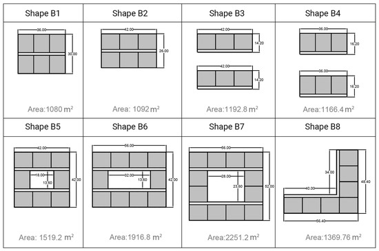
Figure 1.
First set of shape alternatives with dimensions based on a base 12 × 14 m2 unit.
Shape B5 (8 modules) represents an evolution of Shape B3, designed not only to maintain the efficient lighting and ventilation features of B3 but also to create a cohesive office building that is accessible throughout. It incorporates a semi-public open space at its center through the addition of a courtyard. This concept progresses to Shape B6 (10 modules), which expands east–west to include additional office modules and enhance the light-receiving façade. Shape B7 (12 modules) retains the width of the north and south façades while adding more modules, thereby increasing the usable office space. The inclusion of the courtyard enhances the human scale of the building’s design, bringing together larger office modules, a principle that reflects contemporary office and commercial structures in Hamburg. This method enhances the relationship with the urban environment, encouraging a community feeling and preventing the building from being seen as an isolated structure. Finally, Shape B8 (7 modules) follows a linear configuration of modules arranged in an L-shape. The east–west wing benefits from daylight through both the north and south façades, while the north–south wing receives light only from its shorter façades facing north and south.
The addition of modules also helps to investigate the effect of increased GFA on environmental outcomes. The shapes are examined at three different heights to further explore the influence of height and increased GFA while maintaining consistent land use.
The second set of buildings shown in Figure 2 focuses on five polygonal and one circle plan shapes, all sharing the same GFA of 1000 m2. These are a set of fundamental geometric shapes, namely square, pentagon, hexagon, heptagon, octagon, and circle, that explore the mere impact of plan shape on environmental impacts.
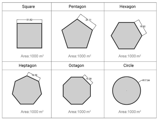
Figure 2.
Second set of shape alternatives with dimensions with a fixed area of 1000 m2.
2.2. Energy Demand Calculation
2.2.1. Energy Demand for Heating and Hot Water
The energy demand of the introduced building shapes was calculated based on the instructions in the DIN 18599 guideline [31].
According to this guideline, the main factors to consider, while calculating the annual heat demand Qh,b per square meter, are given in Equation (1).
The totals of heat sinks and heat sources need to be compared and adjusted according to Equation (1) depending on their utilization levels. For our study, which is an office building, considerations regarding scaled-back operations on weekends/holidays and nights when the office is not used by any occupants should be included in the calculations. The heat stored and utilized during these reduced usage times () should be subtracted from the sums of heat sinks and sources for balancing.
Based on Equation (2), the heat sinks are calculated:
In which:
Qsink: the sum of the heat sinks of the building zone
QT: the transmission heat sinks
QV: the ventilation heat sinks
QIs,sink: the internal heat sinks in the building zone
QS: the heat sinks through radiation, taking solar radiation into account
: the heat stored on days with normal heating operation, which is released from the components on days with reduced operation
Transmission heat flows (QT) are either heat sinks or heat sources, depending on the temperatures on both sides of the building envelope. In the case that the inner temperature is higher than the outside temperature, the transmission is considered a sink, and if it is the other way around, it is considered a heat source.
Ventilation heat flows (QV) occur as a result of infiltration through joints and leaks, through window ventilation and through ventilation via mechanical ventilation systems. Depending on the temperature of the incoming air, the heat flow is either a heat sink or a heat source.
The internal heat sinks (QIs,sink) can be calculated through Equation (3):
In which:
QI,sink,c: the cold input through cooling systems
QI,sink,fac: the cold input through devices
QI,sink,goods: the cold input from goods
For the case of our building, as an office located in Hamburg, the QI,sink is equal to 0.
The heat flow through radiation (QS) is either a heat sink or a heat source for each component. Heat sinks through radiation can occur when there is low solar radiation and high radiation.
With reduced heating operation on weekends and holidays, the heat can be released from the components during reduced operation times and the heat stored on days of normal operation. This effect is calculated as .
The total amount of heat sources (Qsource), on the other hand, is calculated through Equation (4):
In which,
QS: the heat sources due to solar radiation
QT: the transmission heat sources
QV: the ventilation heat sources
QI,source: the internal heat sources
The internal heat sources can be calculated using Equation (5):
In which,
QI,source,p: the heat input by people
QI,source,l: the heat input from artificial lighting
QI,source,fac: the heat input from devices and machines
QI,source,goods: the heat input from goods
QI,source,h: the heat input through heating and cooling systems
Depending on the usage profile, the heat given off by people is specified and expressed as an area-related value. The amounts of heat generated by the operation of electrical devices and machines (such as computers, servers, printers) in the building zone are also specified based on the usable area. For rough balancing, QI,source,h is set to zero. Determining the heat input from artificial lighting (QI,source,l) is based on calculations explained in Section 2.2.3.
As heat sources (Qsource) are directly associated with solar gains (QS), as indicated in Equation (4), we need to define a geographical location for the building to be able to gain weather and solar radiation data insights. This is also true for the calculation of heat losses according to Equation (2), which includes both transmission heat loss and ventilation heat loss.
- Geographical context
Hamburg, the second largest city in Germany and the largest in Northern Germany, was chosen for this study due to its unique features as a major port city situated on the Elbe River, with proximity to the North Sea. Hamburg’s climate, categorized under the “cool humid” type based on Ashrae 169 [38], features mild winters and moderately warm summers. The region’s climate varies significantly due to the alternating dominance of maritime and continental air masses. The high heat capacity of water helps moderate temperatures, resulting in relatively stable seasonal changes. Observations over more than a century show variations in precipitation, temperature, and sunshine, reflecting both short-term fluctuations and long-term changes in weather patterns [39].
Regarding solar conditions, Hamburg receives a moderate amount of sunlight throughout the year, with longer daylight hours in the summer months and shorter days in winter. Cloud cover can vary, impacting the intensity of sunlight reaching the city.
The average outside temperature for different months of the year based on data provided in DIN 18599-10 [29] is presented in Table 2. Following that, Table 3 provides the solar intensities for each month, categorized by four main sides of the building facade.
Table 2.
Average monthly outside air temperatures for the reference location Hamburg, DIN 18599-10 [29].
Table 3.
Mean monthly solar radiation intensities for the reference location Hamburg, DIN 18599-10 [29].
- Shape-related factors
Based on the provided explanation on how the heat demand of the building is calculated, along with additional equations introduced in this section, we can identify the following factors that are influenced by the shape of the building, followed by factors that influence the heat demand but are independent from the shape of the building.
Transmission heat flows (QT): The heat transfer through the building envelope, comprising the walls, roof, floor, and windows, can be calculated using Equation (6). This transfer is influenced by factors such as the surface area, orientation, and insulation of these components. The impact of each of these factors is accounted for through the transmission heat transfer coefficient (HT,j). It is expected that buildings with larger surface areas or less insulation may have higher transmission heat flows, leading to higher heat demand. The following equation shows how this value is incorporated into QT:
HT,j: the transmission heat transfer coefficient between the building zone and an adjacent area
: the internal temperature balance of the building
: the average monthly outdoor temperature or the average temperature in an adjacent zone
: the duration of calculation period
Ventilation heat flows (QV): The infiltration of outside air through joints, leaks, and ventilation systems contributes to heat exchange with the indoor environment. The design and layout of the building, including the number and size of windows and doors, can influence ventilation heat flows. Buildings with more windows or less airtight construction may experience higher ventilation heat flows and consequently higher heat demand. The impact of these design elements is accounted for through the ventilation heat transfer coefficient (HV,k). The ventilation heat flows are calculated through Equation (7).
: the ventilation heat transfer coefficient for ventilation from outside, another building zone, or through a ventilation system
: the internal temperature balance of the building zone
: the average monthly outside temperature or the average temperature of the air from another building zone or the average temperature of the supply air of the ventilation system
: the duration of calculation period
Solar radiation (QS): Solar radiation affects heat exchange through the building envelope, particularly through windows. The orientation, size, and shading of windows determine the amount of solar heat gain or loss. Buildings with more windows, larger window areas, or poor shading are expected to experience higher solar radiation heat flows and thus higher heat demand. Solar radiation can be calculated using Equation (8) or (9) based on whether it is a heat source or a sink:
: external heat transfer resistance
: thermal transmittance of component
: the total area of the component in one orientation
: the absorption coefficient of the component for solar radiation
: the global solar radiation for the orientation of the component surface
: the form factor between the component and the sky
: the external radiation coefficient
: the mean difference between the temperature of the ambient air and the apparent temperature of the sky
: the duration of the calculation period
- Non-shape-related factors
Occupancy profile (QI,source,p): The heat generated by occupants within the building depends on factors such as occupancy density, activity levels, and internal heat gains from metabolic processes. Buildings with more occupants or higher activity levels have higher internal heat sources from people, leading to higher heat demand.
Artificial lighting (QI,source,l): The heat generated by artificial lighting systems depends on factors such as lighting efficiency, usage patterns, and the type of lighting technology used. Buildings with more extensive lighting systems or longer operating hours have higher heat sources from artificial lighting, contributing to higher heat demand.
The demand for artificial lighting in the building is partly influenced by the distribution of daylight within the building. Areas that receive ample daylight require less artificial lighting compared to areas with limited or no access to natural light. This relationship is closely tied to the dimensions and placement of windows, making it a shape-related factor. Further details regarding the shape-related aspects of this factor will be discussed in Section 2.2.3.
Devices and machines (QI,source,fac): The heat generated by electrical devices and machines within the building depends on factors such as the number, type, and usage patterns of these devices. Buildings with more electronic equipment or higher usage levels are expected to have higher heat sources from devices and machines, leading to higher heat demand.
Goods (QI,source,goods): The heat generated by stored goods within the building depends on factors such as the type of goods, storage conditions, and quantity of goods. Buildings with more stored goods or goods that require temperature control such as computers and servers have higher heat sources from goods, contributing to higher heat demand.
Heating and cooling systems (QI,source,h): The heat generated by heating and cooling systems within the building depends on factors such as system efficiency, setpoint temperatures, and usage patterns. While QI,source,h is set to zero for rough balancing in the given case, in other scenarios, the efficiency and usage of heating and cooling systems can influence heat demand.
Energy demand for hot water
Derived from DIN 18599-10 [29], the calculation process for determining the energy requirements of domestic hot water for an office building (qw,b,d) includes multiplying the predefined amount of 30 Wh/(m2d) by the number of building operation days throughout the year, which in this case is equal to 250.
2.2.2. Window-to-Wall Ratio (WWR)
Several studies [40,41,42,43,44] have investigated the optimal ratio of windows to walls for office buildings in different climates, aiming to adjust energy utilization and enhance overall building performance. Understanding the WWR is crucial as it plays a pivotal role in shaping the energy dynamics of a building, influencing factors such as natural light delivery depth, heat gain, heat loss, thermal comfort, and HVAC load. In the following section, we review a few of these studies that are relevant to our study.
In the cold climatic setting explored in a study by Shaeri et al. [45], it was observed that the building’s minimum energy consumption varied across different facade orientations and window percentages. For instance, the northern facade exhibited the lowest energy consumption, at 20% and 30% window coverage, compared to higher window percentages. Similarly, the southern facade achieved its minimum energy consumption within the range of 20% to 60% window coverage. The east facade demonstrated decreased energy consumption, at 50% and 60% window coverage, while the west facade exhibited its minimum annual energy consumption at 60% window coverage.
In a study by Ghisi and Tinker [46] examining room sizes and ratios, the findings indicated that smaller rooms and those with wider dimensions exhibit higher potential for energy savings on lighting, primarily attributed to increased daylight penetration through windows. This effect is attributed to the larger window-to-floor ratio typically found in smaller rooms. Additionally, rooms with a greater width are observed to offer greater energy savings on lighting, attributed to the combined utilization of natural and artificial lighting. Furthermore, the study suggests that the optimal window area tends to be larger in orientations with lower energy consumption, considering the reduced solar thermal loads reaching the facade. This phenomenon enhances the potential for energy savings through daylighting contributions.
In a comprehensive study employing a multitude of integrated thermal lighting simulations, along with a sensitivity analysis, Goia [47] identified suggested ranges for the WWR surrounding the optimal value across different climates and orientations. The findings revealed that the optimal WWR values typically fell within a relatively narrow range, approximately between 0.30 and 0.45, even when considering buildings situated in vastly divergent climates. The study concluded that the selection of the optimal WWR is less critical for south-facing facades compared to north-, east-, and west-facing facades in warm climates, stating that incorrect WWR choices can lead to a higher increase of up to 25% in total energy usage compared to south-facing facades. The optimal WWR of windows of a sample building was calculated for four different locations of Oslo, Frankfurt, Rome, and Athens. The optimum WWR in the context of Frankfurt was calculated as 0.40 for the south facade, 0.43 for the north facade, 0.41 for the west façade, and 0.39 for the east facade.
With respect to previous studies and having the climatic conditions of Hamburg in mind, the size of windows in our study is considered to be 40% of the exterior facade on the north side and 60% on the south side. Windows are only located on the opposite sides of the north and south facades and have the same width as the facade itself. The lower edge of the window is positioned at a height which in this case is the same as the height of the usable area inside the office, and equal to 0.8m. The height of windows in the southern facade (corresponding to a 0.6 WWR) is equal to 1.6m and in the northern facade (corresponding to a 0.4 WWR) equal to 1.2m.
2.2.3. Energy Demand for Artificial Lighting
The final energy requirements for lighting purposes are to be determined by defining different building zones, and calculation areas [30] using the following Equation (10):
QI,f,n,j can be calculated using Equation (11):
where
QI,f: the final energy requirement for lighting
N: the number of zones
J: the number of areas
Ft,n: the partial operating factor of the building operating time for lighting which is equal to 1 for an open plan office function.
pj: the specific electrical rating power of area j
ATL,j: the partial area of zone j that is supplied with daylight
AKTL,j: the partial area of zone j that is not provided with daylight
teff,Day,TL,j: the effective operating time of the lighting system in the daylight-supplied part of zone j at daytime
teff,Day,KTL,j: the effective operating time of the lighting system in the part of zone j that is not supplied with daylight at daytime
teff,Night,j: the effective operating time of the lighting system in zone j at night
The specific electrical rating power (pj) is calculated through Equation (12). This equation takes into account the electrical rating performance (pj,lx) which is achieved based on the type of lighting, maintenance value of the luminance, and the net floor area. Other parameters include the maintenance value of the illuminance , the adjustment factor for considering the maintenance factor the reduction factor for consideration of the visual task area the lamp adjustment factor for non-linear fluorescent lamps , and the adjustment factor for considering the illumination of vertical surfaces .
An important factor while calculating the artificial light requirements of the building zones are the area of openings, in this case windows on the northern and southern facades that provide daylight into the working area and decrease the need for artificial lighting during daytime hours. For the calculation areas, a subdivision must be made of areas that are supplied with daylight from facades (ATL,j), Equation (13), and those which are not supplied with daylight (AKTL,j).
, being the width of the daylight area in Equation (13), is equal to the width of the facade on which the windows are located. on the other hand, which represents the depth of the daylight area as seen in Equation (14), is dependent on the height of the usage level () which is equal to 0.8m for an open plan office profile and the height of the window top (). is defined for the study shapes based on the WWR achieved from assumptionsdescribed in Section 2.2.2 and is equal to 2.6 m for southern windows and 2 m for northern windows.
The parameters teff,Day,TL,j, teff,Day,KTL,j, and teff,Night,j, in Equation (11) represent the effective operating time and the influence of daylight supply on lighting energy requirements, and are each calculated through distinct methodologies tailored to capture specific aspects of the lighting environment.
Teff,Day,TL,j represents the effective daytime operating time within area j, factoring in various parameters such as partial operating factors and daylight availability. It is calculated by the product of four key parameters: FPrä,j, FKL,j, FTL,j, and tDay,n. Among these, FPrä,j accounts for the presence in the calculation area j, where a value of 1 signifies full presence. FKL,j adjusts for constant light control systems, while FTL,j considers daylight contribution, reflecting the dynamic nature of daylight supply influenced by geographical location, climatic conditions, and structural elements. Finally, tDay,n denotes the operating time of zone n during daylight hours.
The determination of FTL,j, particularly, involves a comprehensive assessment of the available daylight supply and its impact on lighting energy requirements. This evaluation entails categorizing the calculation area into zones with and without daylight supply, classifying daylight supply based on structural parameters, and calculating the proportion of daylight in the required exposure. Through this multi-step procedure, the partial operating factor FTL,j is derived, accounting for both daylight supply and the effectiveness of daylight-dependent lighting control systems.
Similarly, teff,Day,KTL,j and teff,Night,j quantify effective operating times within daytime and nighttime areas, respectively, with distinct considerations for daylight availability. teff,Day,KTL,j reflects the effective operating time in daytime areas not supplied with daylight and is computed through the multiplication of FPrä,j, FKL,j, and tDay,n. Conversely, Teff,Night,j signifies the effective operating time during nighttime, calculated by the product of FPrä,j, FKL,j, and tNight,n, where tNight,n represents the operating time of zone n during nighttime hours.
The artificial lighting energy demand is determined, expressed in kWh/m2·a, through the application of the aforementioned equations and the associated considerations. This calculation incorporates the analysis of relevant parameters, ensuring a complete evaluation of energy requirements per unit area annually.
2.3. LCA Calculation
For the life cycle assessment (LCA) calculation of shapes, the final energy demand results, including energy requirements for heating, hot water, and lighting, are entered into the software based on the assumption that electric heaters will serve as the primary heating systems. The source of electricity for these purposes is considered to be Germany’s electricity grid mix of 2018. According to the ÖKOBAUDAT database, this dataset represents a cradle-to-gate inventory. Electricity in inventory is analyzed based on the specific circumstances of each country and is conducted at various levels. The modeling of the electricity consumption mix takes into account transmission and distribution losses, as well as the energy producers’ own usage. Key contributors to the Germany’s electricity grid mix in 2018 include lignite, wind, hard coal, natural gas, and nuclear energy [36].
The LCA study includes analyses of both energy and material flows; however, this particular investigation concentrates solely on the operational energy phase. Therefore, the values for the calculated indicators exclusively reflect the impacts associated with energy consumption. A reference service life of 50 years has been adopted for the life cycle assessment of the office building.
3. Results
3.1. Heat Demand
Heat demand represents the energy required for heating per square meter of office spaces per year. The final thermal energy demand for various geometries is determined by employing electric heaters as the designated heating system. As discussed in Section 2.2.1, heat demand is influenced by various shape-related and non-shape-related factors. These factors include building shape, floor area, envelope area, window size and location, and climate conditions. The calculated values for various energy demands are gathered in Table 4. Through reviewing and comparing the results, we can identify certain trends. Generally, there is a trend indicating that as the number of stories increases, the heat demand decreases. This can be attributed to the concept of thermal mass and compactness in taller buildings. Taller structures have a higher thermal mass, meaning they can retain heat better than shorter buildings. Additionally, taller buildings have a more compact form, resulting in reduced surface area relative to their volume, which helps minimize heat loss. In our case studies, taller buildings offer energy savings due to their inherent thermal properties. The previous phenomenon can be measured through “form factor” or “heat loss form factor”, which is the ratio of a building’s outer surface area which can lose heat (the thermal envelope) to the floor area that gets heated. The form factor for building shapes B1 to B8 varies from 2.46 to 2.67. This amount is between 1.42 and 1.63 for B1-2 to B8-2 and between 0.9 and 1.1 for shapes B1-4 to B8-4. As a general rule of thumb, out of the given results we can conclude that higher form factors are associated with higher heat demands, and therefore there is a direct relation. The only exception occurs with shape B6, where the form factor is slightly lower than that of B8, yet the heat demand is higher. A similar pattern is observed for B6-2 and B6-4, which have lower form factor values compared to B5-2, B8-2, and B5-4, B8-4, respectively, but demonstrate higher heating demands. For shapes that have almost similar form factor values, the window-to-floor ratio (WFR) seems to be the determinant factor as it directly influences heat gains and losses. A higher WFR results in increased heat loss through the windows, especially during colder months, as windows generally have lower insulation properties compared to walls. Additionally, while larger windows may allow more solar heat gain, this benefit does not always offset the higher heat loss [48]. In this case the WFR for B6 is higher than B8 and therefore the heating demand is higher. This is also applicable to B6-2 and B6-4 both of which have higher WFRs than B5-2, B8-2 and B5-4, B8-4 and therefore show higher heat demands.
Table 4.
The amount of energy required for heating and artificial lighting of first building shape set (Refer to Supplementary Materials for additional data).
The rule also applies to the second set of shapes (square, pentagon, etc.). The form factor ranges between 2.43 to 2.47 for these shapes. Square has the highest surface to floor ratio and the circle has the lowest. Even though the square has the highest form factor, the WFR for this shape is much lower than the other ones and equal to 0.09 and this leads to the lowest heat demand. The same applies for Octagon that has a higher form factor but a lower WFR than Circle shape and therefore lower heat demand.
3.2. Lighting Demand
Analyzing the results across various building shapes reveals a correlation between the lighting demand and WFR in each case.
This relationship is inverse, meaning that for the same floor area, an increase in window area leads to a lower lighting demand. This is evident in the values shown in Table 4 for WFR and Lighting demand of shapes B1 to B8. In the case of different heights in these shapes, as the height of a building increases within a specific shape category, there is a corresponding increase in the total window area. This increase in window area is proportional to the increase in floor area, maintaining a relatively constant window-to-floor area ratio. Consequently, regardless of the building’s height within a particular shape category, the ratio of the window area to floor area remains relatively constant.
It should be noted that our case studies were conducted in a non-continuous urban fabric context, meaning that the shadowing effect of the adjacent buildings are disregarded for the study.
Between the results of the first building set (B1 to B8) ranging from 24.69 to 30.28 , the minimum belongs to shape B3 (having the highest WFR of 0.22) and the maximum belongs to B1 (having the lowest WFR of 0.1).
Between the second building shapes, the highest demand of 30.73 belongs to the square plan shape, with a WFR of 0.09. The lowest demand is equal to 29.93 and belongs to the hexagon shape, with a WFR of 0.18. While the WFR for the pentagon shape is higher than that of the hexagon, the demand for the pentagon is slightly higher. This inconsistency is due to the fact that for the polygon and circle shapes, the buildings’ faces on which the windows are located are not exactly directed towards north or south directions. Therefore, while the area of the window might be higher, that side of the building might have a lower lighting depth () and delivers a lower amount of light to interior spaces compared to the other cases.
3.3. Hot Water Demand
The hot water demand remains consistent across all building shapes studied. This uniformity can be attributed to the standardized approach to hot water usage assumed in our analysis. Regardless of the specific building shape or its dimensions, we assumed a consistent level of hot water demand per unit of floor area. This assumption implies that factors such as building height, floor area, and window area do not influence hot water consumption in our models. Therefore, the hot water demand remains constant and equal to 7.5 across different building shapes, allowing for direct comparisons of other energy and environmental performance metrics between cases.
3.4. Total Energy Demand
The data in Table 4 and Table 5 reveal a major trend regarding the total energy demand including lighting, heating, and hot water across different building shapes. While larger WFRs contribute to slight decreases in lighting demand, the dominant factor influencing the total energy demand is heating. For lighting demand, the effect of the WFR is apparent, with shapes having more windows per floor area exhibiting lower lighting demand due to increased natural daylight penetration. However, when considering the total energy demand, the influence of heating demand becomes more pronounced. Heating demand tends to follow the reverse rule, wherein shapes with more windows experience higher heat loss through transmission and ventilation, resulting in higher heating demand. This effect outweighs the reduction in lighting demand due to increased window area, leading to an overall increase in total energy demand. This emphasizes the importance of balancing window design to optimize energy performance across all aspects of building energy consumption. Table 4 shows the amount of energy required for heating, hot water, and artificial lighting of the first building shape set and Table 5 summarizes these energy requirements for the second building shape set.
Table 5.
The amount of energy required for the heating and artificial lighting of the second building shape set (Refer to Supplementary Materials for additional data).
Amongst the shapes listed, the shape with the highest total energy demand is B3 with a value of 135.59 , while the shape with the lowest total energy demand is B1-4 with a value of 77.14 . The second set of shapes, having a shape factor of 2.4, have a variation of 125.72 to 131.64 in the amount of total energy demand.
Based on the results gathered from heat demand and lighting demand, we can conclude that the interplay of outer surface area and window area in relation to the net floor area of the building plays a major role in determining the final energy demand of different shapes.
It should be noted that cooling demand was not considered for calculating the total energy demand in this investigation. Additional individual physical phenomena affecting the total energy demand like cooling by wind or precipitation were also neglected.
3.5. Environmental Impacts
In examining the impacts of different building shapes, we chose to focus on two specific categories: (1) Climate change that is represented by the GWP indicator and falls under environmental impacts and (2) PENRT that falls under used resources.
GWP, expressed as a midpoint indicator in units of kg CO2 equivalents/m2a, represents the cumulative impact of greenhouse gases including carbon dioxide, methane, nitrous oxide, and others, translated into CO2 equivalents to quantify their contribution to the greenhouse effect [49]. During the operational phase, buildings primarily consume energy for heating, cooling, lighting, and powering appliances. This energy use leads to substantial greenhouse gas emissions and resource depletion, particularly when the energy source is fossil fuels. As a result, GWP and PENRT, representing those impacts, are essential metrics for evaluating a building’s environmental footprint throughout its operational lifespan. The essentiality and commonality of these indicators is evidenced by several resources [19,22], including Hauschild et al. [49], who highlight in their book that these two indicators are among the most commonly used in LCA studies.
The observed range for GWP, spanning from 42.14 to 74.08 kgCO2 equiv./m2NFA·a (net floor area) for the first set of shapes, highlights the considerable potential for reducing CO2 emissions by optimizing building shapes. Starting with the one-story building shapes, Figure 3 shows the GWP for shapes B1 to B8. The shapes B1 through B4 are designed to incorporate an identical number of 12 × 14 modules, totaling six modules each. The major difference between these four models is their compactness, measured as their form factor. Shapes B3 and B4 have form factors equal to 2.67 and 2.64. Shapes B1 and B2, on the other hand, exhibit lower values of 2.46 and 2.47, indicating smaller outer surface areas compared to the previous two shapes. This reduction in the outer surface area results in a decreased heat demand, which, by reducing the consumption of energy resources, leads to a lower GWP. This means that over 5 kg of CO2 equivalent per square meter per year can be saved through taking a more efficient design decision. This is a total saving of 13.91 tons CO2 equiv./a by selecting shape B1 over shape B3.
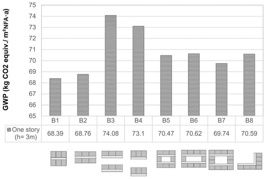
Figure 3.
The GWP (kg CO2 equiv./m2NFA·a) of one-story building shapes.
Figure 4 shows the GWP of all the building shapes in set one. The statistics in this image show the huge contribution of increasing heights to GWP deduction. Looking at shape B1, an increase in the height to two stories (B1-2) decreases the GWP by 17.28 kgCO2 equiv./m2NFA·a, while an increase to four stories (B1-4) results in a reduction of 26.25 kgCO2 equiv./m2NFA·a in GWP. This means that if there are two options of either having two/four separate one-story buildings on the ground or one single building with two/four stories, the second option is more favorable in terms of environmental performance. Opting for shape B1-2 instead of two separate buildings of shape B1 saves a total CO2 equiv. of 35.83 tons/a, and choosing a four-story building (B1-4) instead of four separate B1 buildings saves a total of 108.84 tons/a of CO2 equiv. This trend is consistent across all other shapes, where an increase in height leads to reductions in CO2 equiv. emissions. However, as the evidence suggests, this decrease in emissions per square meter does not follow a linear trend and the reduction in CO2 equiv. emissions diminishes as additional stories are added.
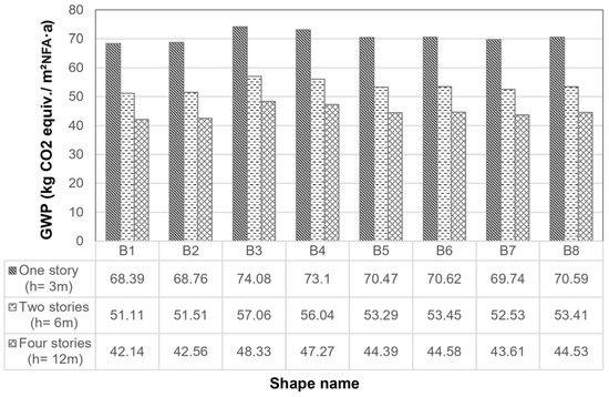
Figure 4.
The GWP (kg CO2 equiv./m2NFA·a) of different building shapes with three different heights.
Figure 5 presents the GWP values for the second set of building shapes. The range varies between the lowest amount of 68.68 kgCO2 equiv./m2NFA·a for the square and the highest amount of 71.92 kgCO2 equiv./m2NFA·a for the pentagon. The lowest GWP value of the square can be attributed to the lowest window areas in the building surface (WFR of 0.09), which is responsible for the lowest exchange of heat in the form of gains and losses compared to other shapes, and therefore leads to a lower total energy demand of the building. The pentagon, hexagon, heptagon, and circle having almost similar WFRs of 0.19, 0.18, 0.17, and 0.17 show lower differences in terms of their GWP values. Under the assumptions of this study, selecting a square plan with windows only on the north and south sides, over a pentagonal plan shape, can result in a CO2 equiv. savings of 3.1 tons per year.
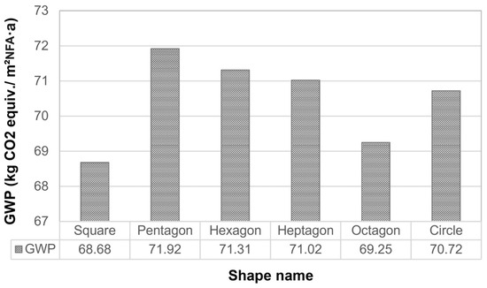
Figure 5.
The GWP (kg CO2 equiv./m2NFA·a) of different building shapes.
As well as GWP, the range for PENRT, varying from 524.95 to 922.67 MJ/m2NFA·a, underscores the importance of shape-related decisions in enhancing energy efficiency and resource conservation. Figure 6 shows the values of PENRT for different shapes in set one. As the evidence shows, PENRT has a direct relation to the total energy demand, meaning that the higher the total energy demand gets, the higher the use of non-renewable primary energy will be. In the first set, buildings with one story height have a value range between 851.84 MJ/m2NFA·a and 922.67 MJ/m2NFA·a, respectively, belonging to shapes B1 and B3. The addition of a story to these buildings causes a drop of over 211 MJ/m2NFA·a in all of the shapes’ PENRT values. An increase in stories from two to four, however, only results in a drop of about 108 MJ/m2NFA·a. Based on a comparison of the results, we conclude that the number of stories does not exhibit a linear relationship with the environmental impacts.
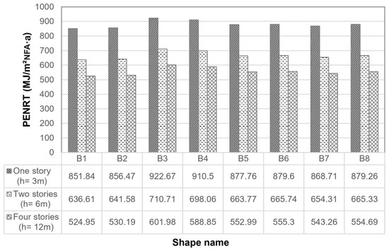
Figure 6.
The PENRT (MJ/m2NFA·a) of different building shapes with three different heights.
Between the four shapes (B1 to B4), all of which have the same number of office units (6 modules of 12 × 14 m), shape B1 shows the best results in terms of PENRT by having a value of 851.84 MJ/m2NFA·a. This means that a simple rearrangement of office units in planning can save about 70.83 MJ/m2NFA·a or 173.35 GJ (gigajoules)/a in total. The effect of the story addition is more recognizable when we have a comparison between the option of a multi-story building and a hypothetical version where multiple buildings with the same shape are located closely but separately in a horizontal arrangement. For example, when considering shape B1-2 (two stories), the difference in energy demand between this option and having shape B1 (one story) duplicated in a horizontal arrangement is 446.28 GJ per year. The difference between shape B1-4 and four horizontally arranged B1 shapes in terms of PENRT is equal to 1355.65 GJ/a. The comparisons show a notable difference between different studied options caused merely by their shape.
The PENRT values for the second shape set are indicated in Figure 7. The pentagon, with 895.79 MJ/m2NFA·a, has the highest value and the square has the lowest with a value of 855.44 MJ/m2NFA·a. It is observed that with an increase in the number of sides from pentagon to octagon, the amount of PENRT decreased. This trend is evidently attributed to a decrease in WFR. As mentioned in Section 3.4, an increase in the area of windows in relation to the net floor area causes an increase in heat loss and majorly affects the total energy demand, even though it might slightly decrease the lighting demand. The circle having a WFR almost similar to the heptagon shows nearly the same PENRT value as the heptagon. In the case of the square, the lowest PENRT is a result of the lowest WFR, as this shape has only two sides with windows on them, facing north and south. The difference in the value of PENRT between the pentagon and square is 40.35 MJ/m2NFA·a, and taking into account the m2NFA·a of 960m2 for both shapes, the total difference would be equal to 38.73 GJ/a.
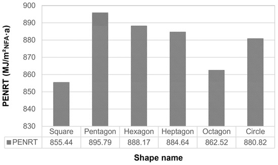
Figure 7.
The PENRT (MJ/m2NFA·a) of different building shapes.
4. Discussion
As observed, both GWP and PENRT exhibit a direct relationship with total energy demand. This correlation underscores the significance of shape-related factors influencing the energy consumption and subsequent environmental impacts of buildings.
The findings of the study regarding the first set of shapes confirm the relationship between form factor, indicative of a building’s compactness, and its environmental impacts, particularly concerning operational energy, while also being influenced by WFR. The ranking of shapes in terms of form factor is as follows: B1 < B2 < B7 < B5, B6 < B8 < B4 < B3, with respective values of 2.46, 2.47, 2.52, 2.55, 2.55, 2.56, 2.64, and 2.67. Based on the results, although there is a slight difference, the rankings for GWP and PENRT follow the same order: B1 < B2 < B7 < B5 < B8 < B6 < B4 < B3. This discrepancy shows that when form factors are similar or very close, as seen with B5, B6, and B8, the size of the windows relative to the usable floor area plays the main role in determining which shape results in greater environmental impacts due to increased energy consumption. The WFR rankings for these three shapes are: B5, B8 < B6, with corresponding values of 0.12, 0.12, and 0.14.
From an architectural perspective, shapes B3 and B4 are more favorable than B1 and B2 for providing adequate daylight and natural ventilation to interior spaces, as well as for creating a connection to the urban context through the central pathway. However, due to their large outer surface areas and high potential for heat exchange with the environment, these shapes yield the worst results from a life cycle perspective. The performance improves when transitioning to courtyard designs. By reducing the form factor of shapes B3 and B4, better alternatives, such as designs B5 to B7, can be achieved. These designs incorporate a central courtyard that fosters a connection to the urban fabric while maintaining favorable lighting and ventilation conditions. Moreover, increasing the number of modules does not necessarily lead to higher GWP or PENRT per square meter, provided the compactness of the building remains constant. Instead, the observed difference lies in the building’s total environmental footprint. Our analysis confirms that heating demand is the dominant factor in operational energy consumption, aligning with previous studies [9,10] that emphasize thermal performance as a key driver of energy efficiency. We also examine the impact of window size in relation to floor area, demonstrating how larger proportions, while architecturally desirable, increase heat loss despite reducing artificial lighting demand. Our findings highlight that heat loss has a significantly greater influence on total energy consumption than lighting reductions.
Additionally, our study reinforces the superior life cycle performance of taller buildings, consistent with Foraboschi et al. [27]. However, while their research focuses solely on embodied energy in high-rises, we address the gap by prioritizing operational energy. Our results suggest that vertical expansion offers greater sustainability benefits than horizontal expansion, strengthening its role in urban planning.
While Treloar et al. [26] analyzed five real-built cases, the reliance on existing buildings may introduce challenges in establishing a consistent comparative framework. In contrast, our research systematically evaluates shape-related environmental impacts. By integrating plan layouts and spatial arrangements, we provide deeper insights into design trade-offs. This is particularly relevant in the context of internal courtyards, which not only enhance urban connectivity by creating semi-public spaces but also introduce new thermal performance variables.
The relationship between compactness and environmental performance observed in our study aligns with Lotteau et al. [25], who linked building geometry to EE and carbon emissions. However, their research focused on concrete collective housing within a specific national context. Our study expands on these insights by incorporating operational energy and a broader range of office building typologies. Similarly, Leskovar et al. [22] emphasized avoiding single-story buildings with high shape factors from a material choice perspective; our findings extend this argument by confirming its relevance to energy performance as well. In line with Serrano and Álvarez [21], who demonstrated the economic and ecological advantages of compact multi-family housing, our research underscores the urban and environmental benefits of integrated courtyards in office buildings.
Moreover, by introducing polygonal plan shapes, our study presents new opportunities for research into unconventional geometries and their environmental implications. By isolating shape as a variable and incorporating office-specific factors such as space arrangement, user density, and operational patterns, we provide a foundation for future studies on sustainable office design.
In the course of this study, certain boundaries were set to focus on the key aspects of building energy performance, suggesting the potential for future research. The role of materials in life cycle assessment results was not within the scope of our analysis. Future research could build upon this by exploring the impact of material choices in combination with energy use, to enhance the robustness of sustainability assessments. Our focus on the building operational energy (B6) stage allowed for a targeted investigation of energy use, though expanding the scope to include additional life cycle stages could provide a more holistic perspective on building performance. Similarly, while the exclusion of electricity demand for mechanical ventilation and cooling during the cooling period streamlined our analysis, further research could explore these factors to enrich the understanding of energy consumption patterns. The decision to place windows exclusively on the north and south facades was deliberate. However, exploring alternative window placement strategies could provide valuable insights into optimizing daylighting and energy efficiency and their impacts on environmental performance of the building.
It is essential to recognize that our findings are specific to the climatic context of Hamburg. Future research endeavors could investigate how similar methodologies might yield different results in diverse climatic regions, enhancing the generalizability of our findings.
5. Conclusions
Through the analyses of heat demand, lighting demand, hot water demand, total energy demand, and environmental impacts across various building shapes, our study reveals insights that can inform future architectural and sustainability decisions.
The investigation into heat demand highlighted the interplay between building shape, size, window size, window placement, and climate conditions. Notably, taller structures exhibited lower relative heat demand [] due to their enhanced thermal mass and compact form, illustrating the importance of considering these factors in energy-efficient building design. Furthermore, our findings underscored the significance of the WFR in shaping heating demand, emphasizing the need for thoughtful window sizing and placement strategies to optimize energy performance.
Similarly, the analysis of lighting demand revealed a correlation between the WFR and lighting requirements, with larger window areas contributing to reduced lighting demand. However, the impact of heating demand emerged as a dominant factor in determining total energy demand, underscoring the importance of balancing window design to achieve overall energy efficiency.
Environmental impact assessments, focusing on GWP and PENRT, underscored the significant role of building shape in mitigating carbon emissions and resource depletion. Optimal building designs, characterized by compactness and efficient use of space, demonstrated notable reductions in CO2 equiv. emissions and energy consumption.
In conclusion, our study provides insights into the relationship between building shape, energy performance, and environmental impacts. By integrating these findings into architectural design and urban planning processes, we can prepare for more efficient, and environmentally conscious built environments.
Supplementary Materials
The following supporting information can be downloaded at: https://www.mdpi.com/article/10.3390/su17041659/s1, File S1: Supplementary file.
Author Contributions
S.S. contributed to methodology and concept development, formal analysis and investigation, visualization, use of software, writing of the original draft, and review and editing. I.W. contributed to proposing the research topic, conceptualization, methodology, writing—review and editing, project administration, and supervision of the work. All authors have read and agreed to the published version of the manuscript.
Funding
This research received no external funding.
Data Availability Statement
The original contributions presented in this study are included in the article. Further inquiries can be directed to the corresponding author.
Conflicts of Interest
The authors declare no conflicts of interest.
References
- Ma, M.; Zhou, N.; Feng, W.; Yan, J. Challenges and opportunities in the global net-zero building sector. Cell Rep. Sustain. 2024, 1, 100154. [Google Scholar] [CrossRef]
- Venkatraj, V.; Dixit, M.K.; Yan, W.; Lavy, S. Evaluating the impact of operating energy reduction measures on embodied energy. Energy Build. 2020, 226, 110340. [Google Scholar] [CrossRef]
- Optis, M.; Wild, P. Inadequate documentation in published life cycle energy reports on buildings. Int. J. Life Cycle Assess. 2010, 15, 644–651. [Google Scholar] [CrossRef]
- Dilsiz, A.D.; Felkner, J.; Habert, G.; Nagy, Z. Embodied versus operational energy in residential and commercial buildings: Where should we focus? J. Phys. Conf. Ser. 2019, 1343, 012178. [Google Scholar] [CrossRef]
- Nicholson, S.; Ugursal, V.I. A lifecycle assessment-based environmental analysis of building operationally energy efficient houses in Nova Scotia. J. Build. Eng. 2023, 76, 107102. [Google Scholar] [CrossRef]
- Hemmati, M.; Messadi, T.; Gu, H.; Hemmati, M. LCA Operational Carbon Reduction Based on Energy Strategies Analysis in a Mass Timber Building. Sustainability 2024, 16, 6579. [Google Scholar] [CrossRef]
- Asdrubali, F.; Baldassarri, C.; Fthenakis, V. Life cycle analysis in the construction sector: Guiding the optimization of conventional Italian buildings. Energy Build. 2013, 64, 73–89. [Google Scholar] [CrossRef]
- Hafner, A. Contribution of timber buildings on sustainability issues. In Proceedings of the World Sustainable Building 2014, Barcelona, Spain, 28–30 October 2014. [Google Scholar]
- Moayedi, F.; Zawawi, N.A.W.A.; Liew, M.S. Life Cycle Analysis of Operational Energy in Office Projects Toward Sustainability Practices in the Malaysian Construction Industry. Int. J. Eng. Technol. 2018, 7, 39. [Google Scholar] [CrossRef][Green Version]
- Grygierek, K.; Ferdyn-Grygierek, J. Analysis of the Environmental Impact in the Life Cycle of a Single-Family House in Poland. Atmosphere 2022, 13, 245. [Google Scholar] [CrossRef]
- Hester, J.; Miller, T.R.; Gregory, J.; Kirchain, R. Actionable insights with less data: Guiding early building design decisions with streamlined probabilistic life cycle assessment. Int. J. Life Cycle Assess. 2018, 23, 1903–1915. [Google Scholar] [CrossRef]
- Crawford, R.H.; Czerniakowski, I.; Fuller, R.J. A comprehensive model for streamlining low-energy building design. Energy Build. 2011, 43, 1748–1756. [Google Scholar] [CrossRef]
- Marsh, R. LCA profiles for building components: Strategies for the early design process. Build. Res. Inf. 2015, 44, 358–375. [Google Scholar] [CrossRef]
- Asadi, S.; Amiri, S.S.; Mottahedi, M. On the development of multi-linear regression analysis to assess energy consumption in the early stages of building design. Energy Build. 2014, 85, 246–255. [Google Scholar] [CrossRef]
- Yu, H.; Yang, W.; Li, Q.; Li, J. Optimizing Buildings’ Life Cycle Performance While Allowing Diversity in the Early Design Stage. Sustainability 2022, 14, 8316. [Google Scholar] [CrossRef]
- Basbagill, J.; Flager, F.; Lepech, M.; Fischer, M. Application of life-cycle assessment to early stage building design for reduced embodied environmental impacts. Build. Environ. 2013, 60, 81–92. [Google Scholar] [CrossRef]
- Meex, E.; Hollberg, A.; Knapen, E.; Hildebrand, L.; Verbeeck, G. Requirements for applying LCA-based environmental impact assessment tools in the early stages of building design. Build. Environ. 2018, 133, 228–236. [Google Scholar] [CrossRef]
- Hollberg, A.; Ruth, J. LCA in architectural design—A parametric approach. Int. J. Life Cycle Assess. 2016, 21, 943–960. [Google Scholar] [CrossRef]
- Monteiro, H.; Soares, N. Integrated life cycle assessment of a southern European house addressing different design, construction solutions, operational patterns, and heating systems. Energy Rep. 2022, 8, 526–532. [Google Scholar] [CrossRef]
- Van Den Dobbelsteen, A.; Thijssen, S.; Colaleo, V.; Metz, T.J. Ecology of the building geometry—Environmental performance of different building shape. In Proceedings of the CIB World Building Congress 2007, Cape Town, South Africa, 14–17 May 2007; Available online: https://iris.polito.it/handle/11583/1908680 (accessed on 15 November 2024).
- Serrano, A.Á.R.; Álvarez, S.P. Life Cycle Assessment in Building: A Case Study on the Energy and Emissions Impact Related to the Choice of Housing Typologies and Construction Process in Spain. Sustainability 2016, 8, 287. [Google Scholar] [CrossRef]
- Leskovar, V.Ž.; Žigart, M.; Premrov, M.; Lukman, R.K. Comparative assessment of shape related cross-laminated timber building typologies focusing on environmental performance. J. Clean. Prod. 2019, 216, 482–494. [Google Scholar] [CrossRef]
- Moschetti, R.; Mazzarella, L.; Nord, N. An overall methodology to define reference values for building sustainability parameters. Energy Build. 2014, 88, 413–427. [Google Scholar] [CrossRef]
- Pomponi, F.; Moncaster, A. Embodied carbon mitigation and reduction in the built environment—What does the evidence say? J. Environ. Manag. 2016, 181, 687–700. [Google Scholar] [CrossRef] [PubMed]
- Lotteau, M.; Loubet, P.; Sonnemann, G. An analysis to understand how the shape of a concrete residential building influences its embodied energy and embodied carbon. Energy Build. 2017, 154, 1–11. [Google Scholar] [CrossRef]
- Treloar, G.; Fay, R.; Ilozor, B.; Love, P. An analysis of the embodied energy of office buildings by height. Facilities 2001, 19, 204–214. [Google Scholar] [CrossRef]
- Foraboschi, P.; Mercanzin, M.; Trabucco, D. Sustainable structural design of tall buildings based on embodied energy. Energy Build. 2014, 68, 254–269. [Google Scholar] [CrossRef]
- Grossmann, I. Three scenarios for the greater Hamburg region. Futures 2005, 38, 31–49. [Google Scholar] [CrossRef]
- DIN V 18599-10:2018; Energy Efficiency of Buildings—Calculation of the Net, Final and Primary Energy Demand for Heating, Cooling, Ventilation, Domestic Hot Water and Lighting—Part 10: Boundary Conditions of Use, Climatic Data. Deutsches Institut für Normung e.V. (DIN e.V.): Berlin, Germany, 2018.
- DIN V 18599-4:2018; Energy Efficiency of Buildings—Calculation of the Net, Final and Primary Energy Demand for Heating, Cooling, Ventilation, Domestic Hot Water and Lighting—Part 4: Net and Final Energy Demand for Lighting. Deutsches Institut für Normung e.V. (DIN e.V.): Berlin, Germany, 2018.
- DIN V 18599-2:2018; Energy Efficiency of Buildings—Calculation of the Net, Final and Primary Energy Demand for Heating, Cooling, Ventilation, Domestic Hot Water and Lighting—Part 2: Net Energy Demand for Heating and Cooling of Building Zones. Deutsches Institut für Normung e.V. (DIN e.V.): Berlin, Germany, 2018.
- ELCA. Available online: https://www.bauteileditor.de/ (accessed on 15 November 2024).
- ÖKOBAUDAT Manual. Federal Institute for Research on Building, Urban Affairs and Spatial Development (BBSR). 2021. Available online: https://www.oekobaudat.de/fileadmin/downloads/2021-11-29_OEBD-Manual_v2.1.pdf (accessed on 15 November 2024).
- DIN EN 15978:2011; Sustainability of Construction Works—Assessment of Environmental Performance of Buildings—Calculation Method; German version EN 15978:2011. Deutsches Institut für Normung e.V. (DIN e.V.): Berlin, Germany, 2012.
- DIN EN 15804:2012-04; Sustainability of construction works—Environmental product declarations—Core rules for the product category of construction products; German version EN 5804:2012+A1:2013+A2:2019-10. Deutsches Institut für Normung e.V. (DIN e.V.): Berlin, Germany, 2020.
- BBSR. ÖKOBAUDAT. Available online: https://www.oekobaudat.de/ (accessed on 15 November 2024).
- Mumovic, D.; Santamouris, M. (Eds.) A Handbook of Sustainable Building Design and Engineering: An Integrated Approach to Energy, Health and Operational Performance; Earthscan: London, UK, 2013. [Google Scholar]
- Bre, F. Climate-Representative Locations According to the ASHRAE 169-2020 Climate Classification and Within the WMO Region VI (Europe) [Dataset]; Zenodo; CERN European Organization for Nuclear Research: Geneva, Switzerland, 2022. [Google Scholar] [CrossRef]
- Deutscher Wetterdienst. Klimareport Hamburg, Fakten bis zur Gegenwart—Erwartungen für die Zukunft; Deutscher Wetterdienst; Behörde für Umwelt, Klima, Energie und Agrarwirtschaft: Hamburg, Germany, 2021. [Google Scholar]
- Rana, J.; Hasan, R.; Sobuz, H.R.; Tam, V.W.Y. Impact assessment of window to wall ratio on energy consumption of an office building of subtropical monsoon climatic country Bangladesh. Int. J. Constr. Manag. 2020, 22, 2528–2553. [Google Scholar] [CrossRef]
- Troup, L.; Phillips, R.; Eckelman, M.J.; Fannon, D. Effect of Window-to-Wall Ratio on Measured Energy Consumption in US Office Buildings. Energy Build. 2019, 203, 109434. [Google Scholar] [CrossRef]
- Lahmar, I.; Cannavale, A.; Martellotta, F.; Zemmouri, N. The Impact of Building Orientation and Window-to-Wall Ratio on the Performance of Electrochromic Glazing in Hot Arid Climates: A Parametric Assessment. Buildings 2022, 12, 724. [Google Scholar] [CrossRef]
- Yu, Z.; Zhang, W.L.; Fang, T.Y. Impact of Building Orientation and Window-Wall Ratio on the Office Building Energy Consumption. Appl. Mech. Mater. 2013, 409–410, 606–611. [Google Scholar] [CrossRef]
- Ahmed, A.E.; Suwaed, M.S.; Shakir, A.M.; Ghareeb, A. The impact of window orientation, glazing, and window-to-wall ratio on the heating and cooling energy of an office building: The case of hot and semi-arid climate. J. Eng. Res. 2023; in press. [Google Scholar] [CrossRef]
- Shaeri, J.; Habibi, A.; Yaghoubi, M.; Chokhachian, A. The Optimum Window-to-Wall Ratio in Office Buildings for Hot-Humid, Hot-Dry, and Cold Climates in Iran. Environments 2019, 6, 45. [Google Scholar] [CrossRef]
- Ghisi, E.; Tinker, J.A. An Ideal Window Area concept for energy efficient integration of daylight and artificial light in buildings. Build. Environ. 2005, 40, 51–61. [Google Scholar] [CrossRef]
- Goia, F. Search for the optimal window-to-wall ratio in office buildings in different European climates and the implications on total energy saving potential. Sol. Energy 2016, 132, 467–492. [Google Scholar] [CrossRef]
- Ma, R.; Ma, R.; Long, E. Analysis of the rule of window-to-wall ratio on energy demand of residential buildings in different locations in China. Heliyon 2023, 9, e12803. [Google Scholar] [CrossRef] [PubMed]
- Hauschild, M.Z.; Rosenbaum, R.K.; Olsen, S.I. Life Cycle Assessment: Theory and Practice; Springer: Berlin/Heidelberg, Germany, 2017. [Google Scholar]
Disclaimer/Publisher’s Note: The statements, opinions and data contained in all publications are solely those of the individual author(s) and contributor(s) and not of MDPI and/or the editor(s). MDPI and/or the editor(s) disclaim responsibility for any injury to people or property resulting from any ideas, methods, instructions or products referred to in the content. |
© 2025 by the authors. Licensee MDPI, Basel, Switzerland. This article is an open access article distributed under the terms and conditions of the Creative Commons Attribution (CC BY) license (https://creativecommons.org/licenses/by/4.0/).