The Non-Linear Impact of Highway Improvements on the Urban–Rural Income Gap in Underdeveloped Regions: A Mixed-Methods Approach

Abstract

The vast urban–rural income gap (URIG) is a global challenge, particularly severe in underdeveloped regions. While the income-generating effects of transportation improvements are widely accepted, their income distribution effects remain controversial. This study focuses on national poverty-alleviated counties in central and western China, using a mixed-methods approach to quantitatively test the non-linear relationship between highway improvements and the URIG and qualitatively analyze the reasons behind the threshold effects of regional economic development levels. The main findings are as follows: first, regional economic development levels exhibit a double-threshold effect, with the impact of highway improvements shifting from widening to narrowing the URIG after surpassing the second thresholds. Second, inter-regional highways have a limited impact on narrowing the URIG, while intra-regional highways significantly reduce the URIG once crossing their thresholds, reflecting the distinct functions of different highway classes. Third, the heterogeneity analysis reveals that the impact of highway improvements on the URIG varies depending on the external environment surrounding residents, including both the indirect and direct environments. Fourth, from the perspective of rural labor transfer to non-farm employment, regional economic development levels create threshold effects in two ways: for local employment, they influence non-agricultural industry growth and job distribution following highway improvements, affecting rural laborers’ participation; for migrant employment, they impact human capital investment, influencing rural laborers’ skills and wage returns after highway improvements.

1. Introduction

Sustainable development is an important and multidimensional issue. In 2015, the United Nations introduced the 17 Sustainable Development Goals (SDGs), covering environmental, economic, and social sustainability. A key aspect of social sustainability is equity, which aims to ensure that the benefits of development reach all groups, particularly marginalized groups. This concept is embodied in No Poverty (SDG 1) and Reduced Inequalities (SDG 10), which represent significant global challenges. As the largest developing country, China had successfully achieved its goal of eradicating absolute poverty by the end of 2020, largely thanks to the Targeted Poverty Alleviation Strategy. However, income inequality remains a significant challenge in China, with the widening urban–rural income gap (URIG) as a prominent manifestation [1]. China always faces unique challenges in narrowing the URIG due to its large population, vast rural and urban areas, and a distinct dual structure. Data from China’s National Bureau of Statistics indicate that while the ratio of per capita disposable income between urban and rural residents has decreased from 3.4 times in 2008 to approximately 2.4 times in 2023, the URIG still contributes 30% to the national income disparity [2]. Consequently, addressing the URIG in China is more complex and challenging than in other developing countries. Among the various government efforts to narrow this gap, including upgrading the industrial structure, investing in human capital, improving infrastructure, and implementing targeted policies [3,4,5,6], transportation improvements are regarded as a critical strategy.

Globally, many developing countries have recognized the role of transportation improvements in combating poverty and increasing incomes, making significant efforts in this regard. Examples include the Golden Quadrilateral Project in India [7], the Universal Access to Rural Roads Project in Ethiopia [8], and the Road Improvement Project in Cambodia [9]. In China, transportation infrastructure has seen rapid development since the reform and opening-up era, with highways promoted as key projects during the poverty alleviation stage. For the underdeveloped regions that have emerged from absolute poverty, narrowing the URIG and achieving shared prosperity have become the next major challenges. Therefore, whether improvements in transportation infrastructure—a long-term, large-scale project with high investment—can continue to narrow the URIG in these regions has become a central concern. However, due to the complexity and variability of factor mobility between urban and rural areas, existing studies present mixed findings on the impact of transportation improvements on the URIG, including widening [10,11], narrowing [12], or even non-linear changes [13]. This debate is particularly problematic in underdeveloped regions, where the income distribution effects of transportation improvements are less optimistic. Specifically, while transportation improvements are generally expected to boost income, in remote rural areas with poor ecological conditions and lagging socio-economic development, local residents are unable to fully benefit from these improvements due to factors such as limited market access, low human capital, and insufficient supporting resources. As a result, their incomes remain marginal, perpetuating the “spatial poverty trap”—a silent but prevalent feature in many underdeveloped rural regions [14].

The existence of this debate suggests that the relationship between transportation improvements and the URIG may be complex and non-linear, varying according to the unique development conditions of each region. Previous studies have noticed this complexity. For instance, Raychaudhuri and De (2016) [15] used cross-country data to show that the effects of infrastructure improvements on income inequality differ between developed and developing countries, underscoring the need to consider country-specific conditions when evaluating income disparities. Similarly, Zhang et al. (2013) [16] found that economic development and urbanization levels significantly influence how transportation infrastructure investments affect the URIG. This implies that regional economic development levels may be a critical factor in shaping the income distribution effects of transportation improvements, a finding especially relevant to China. Although absolute poverty has been alleviated, significant disparities in regional economic development remain across China. The strategies of rural revitalization and common prosperity emphasize the need for localized and orderly progress. Therefore, it is crucial to assess whether transportation improvements have a measurable impact on the URIG in underdeveloped regions, particularly in terms of the threshold effect of regional economic development levels. This assessment will be key to optimizing future policies, which are essential for achieving the Reduced Inequality Goal. However, existing studies on this issue often lack depth regarding the choice of spatial units and geographical area, the object of research, and the content of analysis, suggesting the need for further research.

In terms of spatial units and geographical area, most existing research has primarily focused on provincial and municipal scales, often selecting developed provinces and cities. This has resulted in a lack of empirical research at the county level, particularly in underdeveloped regions. However, county-level administrative divisions (hereafter called counties) are the fundamental administrative units in China, serving as critical links between urban and rural areas, as well as between industry and agriculture. Moreover, counties in underdeveloped regions face particularly severe challenges, where the URIG was 2.62:1 in 2021, surpassing the national average of 2.5:1. Therefore, examining the URIG at the county level in underdeveloped regions is crucial. In terms of the object of research, highways have acted as crucial connectivity channels in underdeveloped regions because of their adaptability, extensive networks, and integrated systems. These features necessitate multiple highway classifications, allowing for the movement of people and goods on different scales—an aspect highlighted by urban planning scholars [17]. In large countries like China, distinctions among highway classes are especially evident. Nevertheless, these variations have been largely overlooked. In terms of the content of analysis, while some research has examined the non-linear relationship between highway improvements and the URIG, few studies have concentrated on the threshold effect of regional economic development levels. Moreover, there is a lack of in-depth analysis exploring the reasons behind this threshold effect.

This study employs a mixed-methods approach combining quantitative and qualitative research to explore the non-linear impact of highway improvements on the URIG and examine the threshold effect of regional economic development levels in underdeveloped regions of China. It contributes to the existing literature in several ways. First, it focuses specifically on underdeveloped regions, specifically targeting national poverty-alleviated counties in central and western China rather than taking a broad national perspective. In China, regional economic development is typically ranked from east to west, with the central and western regions classified as underdeveloped. Moreover, within these regions, national poverty-alleviated counties represent the regions with the lowest development levels and the greatest challenges in achieving shared prosperity. The term “national poverty-alleviated counties” refers to 832 counties selected from the 2844 countries in China since implementing the Targeted Poverty Alleviation Strategy in 2012. Among these, 756 counties are located in central and western China. Given the marked differences between these counties and the national average, this targeted approach offers relevant insights into their distinct obstacles. Second, the study underscores the interconnected and organized structure of highway systems, classifying them into inter-regional and intra-regional categories. High-grade highways—such as expressways, national highways, and provincial highways—are designated as inter-regional, supporting external connections. In contrast, the rural network—such as county and township roads—is categorized as intra-regional, facilitating internal connectivity within counties. Third, in alignment with the realities of underdeveloped regions, this study goes beyond analyzing the relationship between highway improvements and the URIG. It also addresses the threshold effect of regional economic development levels, investigating the underlying reasons for this effect through field surveys. This approach clarifies the interplay between highway improvements, regional economic development levels, and the URIG.

The rest of this paper is structured as follows: Section 2 presents the literature review and research hypotheses, Section 3 describes the research design, Section 4 contains the analysis of empirical results, Section 5 provides further analysis based on the field survey, and Section 6 concludes with policy implications.

2. Literature Review and Research Hypotheses

2.1. Literature Review

2.1.1. Factors Affecting the Urban–Rural Income Gap

Existing studies on the factors influencing the URIG can be broadly categorized into two groups, namely endogenous factors and exogenous factors. Endogenous factors include urbanization [18], industrial structure [3], digital economy [19], financial development [20], human capital [4], and infrastructure layout [21]. Exogenous factors primarily refer to government policies, such as fiscal policies [22], social security [23], healthcare [24], and government bias in policy-making [5,6]. In China, the URIG is particularly complex due to the long-standing dual economic system. Before the reform and opening-up era, the strict urban–rural household registration (hukou) system and the “scissors” development model between industry and agriculture resulted in a significant URIG, which persists today [25]. The Kuznets inverted “U” curve, which typically explains income inequality trends, does not apply to China’s current context [26]. Recognizing China’s dual economy, scholars have increasingly examined the impact of cross-regional labor migration on the URIG, particularly in light of the gradual loosening of the hukou system.

On the one hand, economic growth and industrial development in cities create numerous employment opportunities, attracting rural laborers to urban areas in search of higher income [27]. This migration offers the potential to narrow the URIG. On the other hand, however, the hukou system restricts migrant laborers’ access to urban public services and confines them mainly to the informal employment sector [28]. This leads to limited job options, decreased employment stability, and a lower willingness to settle permanently in cities [29]. As a result, the inherent advantages of urban residents may actually exacerbate the URIG. Despite these challenges, most studies suggest that labor migration effectively reduces the URIG. First, compared to farmers who remain in agricultural work, migrants can earn higher non-farm income through wage employment or self-employment in non-agricultural industries [29,30]. Second, as surplus laborers leave rural areas, agricultural productivity increases, allowing those who remain in farming to raise their incomes [31]. Additionally, as more rural laborers enter urban non-farm markets, the increased labor supply in certain sectors can reduce wages for urban laborers [32], further narrowing the URIG. In summary, the transfer of rural labor to non-farm employment helps to equalize income returns and reduce the URIG.

2.1.2. Impacts of Transportation Improvements on the Urban–Rural Income Gap

Transportation improvements can accelerate the flow of production factors such as capital, technology, and labor between regions, including between urban and rural areas [33,34], thereby influencing residents’ incomes. However, due to the complexity and variability of factor flows between urban and rural areas, research on the effects of transportation improvements on the URIG has yielded inconsistent results.

Some studies argue that urban and rural areas operate as distinct production regions, with urban areas benefiting from more advanced industrial structures, higher population quality, and more favorable government policies [35]. As a result, urban areas are better positioned to seize the economic agglomeration and industrial transformation opportunities created by transportation improvements, which can widen the URIG. For instance, Calderón and Chong (2004) [10] found that due to the complementarity between infrastructure utilization and individual endowments, transportation investments generate higher returns in wealthier regions. Thus, transportation improvements may exacerbate income inequality between rural and urban areas. Especially in developing countries, studies have shown that transportation improvements often fail to benefit disadvantaged rural areas or provide only minimal advantages, thereby widening the URIG. Examples include Banerjee and Somanathan (2007) for India [36], Bryceson et al. (2008) for Zambia and Vietnam [37], Maia et al. (2016) for Brazil [38], and DaCosta (2013) for China [11].

Other studies suggest that transportation improvements can narrow the URIG. These studies primarily focus on the role of rural labor transfer, suggesting that by enhancing employment opportunities [39] and wage levels [40], transportation improvements may reduce the URIG. In China, rural non-farm employment generally takes two forms, local non-farm employment, where rural labor is transferred within the county, often described as “leaving the land but not the hometown”, and migrant non-farm employment, where rural labor migrates to urban areas, commonly referred to as “leaving the land and the hometown” [41]. Accordingly, transportation improvements impact the non-farm transfer of rural labor in two key ways, thereby affecting the URIG. First, transportation improvements reduce trade costs for production factors and finished goods, facilitating better resource allocation and industrial restructuring across regions [33]. This is particularly beneficial for attracting funds and resources from large cities to underdeveloped regions, where land and labor costs are lower. As a result, local non-agricultural industries grow, absorbing surplus rural labor into local non-farm employment [42]. Second, transportation improvements significantly lower the mobility cost of labor migration, encouraging the cross-regional mobility of surplus rural labor. These laborers enter urban job markets and earn non-farm income [42]. At the same time, the saturation of urban labor markets can reduce wages for urban residents, further narrowing the URIG.

Moreover, given the substantial regional differences within China, studies indicate that the impact of transportation improvements on the URIG varies across regions. For instance, Zhang et al. (2013) [16] found that transportation improvements help reduce the URIG in the eastern regions but exacerbate the URIG in the central and western regions. Kang et al. (2014) [43] demonstrated that highways reduce the URIG across all of China, while railways only impact the eastern regions. Given that the economic development levels in the eastern region are considerably higher than those in the central and western regions, these findings suggest that the income distribution effects of transportation improvements are more pronounced in developed regions than in underdeveloped regions. Similarly, Zhou et al. (2020) [44] argued that rural transportation development significantly reduces the URIG in developed regions but has a negligible effect in underdeveloped regions. Additionally, some studies have identified a non-linear relationship between transportation improvements and the URIG. For example, Ren and Zhang (2013) [13] suggested that the proportion of the rural population influences this relationship. When the rural population is larger, transportation improvements can reduce the URIG by promoting labor migration. However, once rural labor migration reaches a certain level, the impact becomes insignificant.

2.2. Research Hypotheses

The above analysis highlights that rural labor transfer plays a crucial role in reducing the URIG, and transportation improvements significantly influence this process. Therefore, this study, considering the specific conditions in underdeveloped regions, will analyze the threshold effect of regional economic development levels on the relationship between highway improvements and the URIG, primarily from the perspective of rural labor transfer. The existing literature suggests that, ideally, highway improvements can narrow the URIG by promoting rural labor transfer in two ways, namely by (1) reducing trade costs to foster the growth of local non-agricultural industries, thereby providing local non-farm employment opportunities, and (2) lowering mobility cost, enabling rural laborers to move to urban areas for migrant non-farm employment wages. However, in underdeveloped regions, the realization of these ideal outcomes is constrained by specific regional factors.

For local non-farm employment, rural areas in underdeveloped regions face limitations due to a constrained industrial base on the production side and a small consumer market on the consumption side. In contrast, county seats, as local growth centers, benefit from proximity to both low-cost production factors in rural areas and large urban consumer markets. This proximity allows them to fully capitalize on lower trade costs, becoming the primary recipients of modern urban resources following highway improvements, thus facilitating the development of non-agricultural industries and enhancing their capacity to absorb employment. Consequently, urban laborers, with advantages in geographic location, human capital, and information access, are often the first to enter local non-farm job markets and benefit from wage increases. In contrast, rural laborers, who lack these advantages, are less likely to secure jobs in expanding local non-farm industries, missing out on employment opportunities. For migrant non-farm employment, rural residents in underdeveloped regions often face early barriers to capacity development (e.g., education, health) due to prolonged isolation and slow growth, leading to lower skill levels and reduced adaptability to new opportunities in adulthood. While highway improvements provide rural laborers with greater access to external job markets, they still encounter limited employment options and inadequate wage returns. Consequently, the impact of highway improvements on the URIG in underdeveloped regions remains ambiguous, as rural laborers struggle to secure substantial opportunities in local non-farm employment or to achieve meaningful wage returns in migrant non-farm employment.

The participation opportunities for rural laborers to find local employment and the wage returns they earn from migrant employment depend significantly on the saturation of the local job market and individual human capital, both closely linked to regional economic development levels (Figure 1). On the one hand, regional economic development levels dictate the initial job supply and industrial attractiveness in terms of foundational infrastructure, market potential, and business environment. In counties with a solid job supply and high industrial attractiveness, additional abundant jobs generated by highway improvements are layered onto an already substantial job base, creating an undersaturated job market. This not only meets the employment needs of urban laborers but also leaves opportunities for rural laborers. Conversely, if highway improvements add only a limited number of new jobs to regions with an already insufficient job supply, the local job market remains oversaturated, limiting non-farm employment opportunities for rural laborers and hindering efforts to reduce the URIG.

On the other hand, education, both general and vocational, is a critical determinant of human capital, and the equity of educational investment is influenced by regional economic development levels. In regions with higher economic development, governments have more funds and resources, allowing for greater allocation toward rural areas and disadvantaged groups. This supports rural laborers in enhancing their human capital through education, thereby improving their competitive position in urban job markets, securing higher wages, and ultimately narrowing the URIG. In contrast, in underdeveloped regions, limited resources are often concentrated among dominant groups, intensifying the “Matthew effect.” Additionally, early life stages are crucial for human capital formation, and the costs of compensating for missed opportunities during this period are exceedingly high. Therefore, underdeveloped regions have an even greater need for equitable government investment in education, highlighting the threshold effect of regional economic development levels. Based on this analysis, the study proposes the following hypotheses:

Hypothesis 1.

Regional economic development levels have a threshold effect on the reduction in the URIG through highway improvements.

Hypothesis 2.

Regional economic development levels exert a threshold effect by influencing rural laborers’ participation opportunities in local non-farm employment and their wage returns from migrant non-farm employment.

Furthermore, as the most mobile and flexible form of transportation, the core function of highways lies in the coordination and connectivity between different highway classes. Focusing solely on individual highways without considering the network’s overall structure would obscure the actual impacts of highway improvements. Thus, this study further examines the roles of different highway classes. Expressways and national and provincial highways are essential for external connectivity. When inter-regional highway improvements enhance regional accessibility, the economic vitality of counties increases. County seats, which concentrate resources such as population, capital, and policy support, see a rise in employment opportunities and wage levels, resulting in a significant income increase for urban residents. In comparison, although inter-regional highways also improve accessibility for rural areas, the benefits for rural residents are relatively minor. County highways, however, serve a fundamentally different purpose than inter-regional highways. Primarily connecting rural areas to county seats or other key nodes, they are designed to benefit rural residents more than urban residents. As such, county highways play a more significant role in reducing the URIG. Based on this analysis, the study proposes the following hypothesis:

Hypothesis 3.

Intra-regional highways play a more significant role in narrowing the URIG than inter-regional highways.

3. Data, Models and Variables

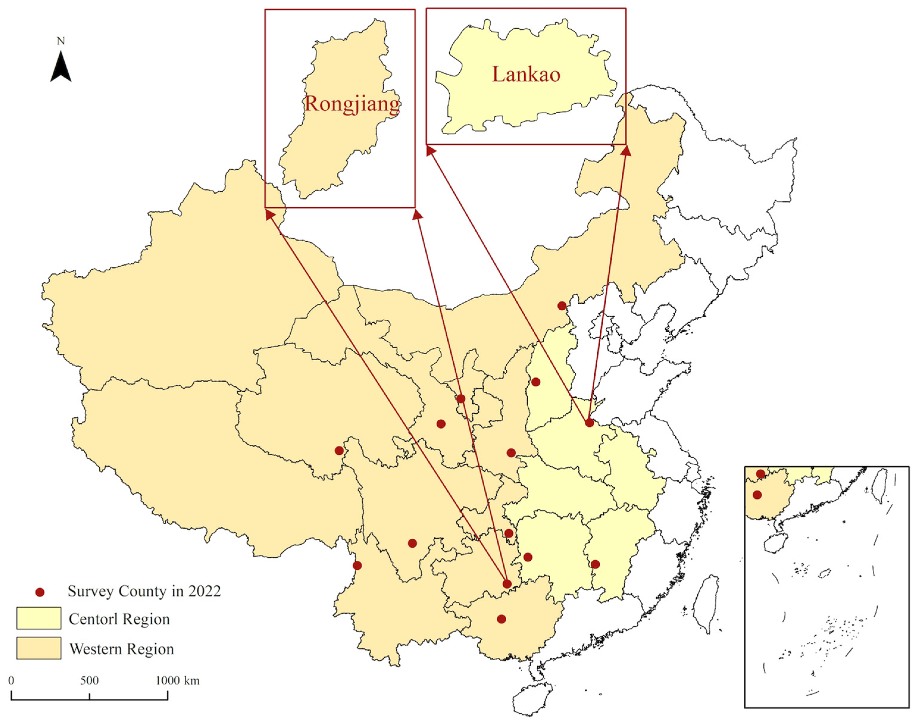
3.1. Data Sources

3.1.1. Quantitative Data

This study focuses on 568 national poverty-alleviated counties in central and western China (this paper follows the convention of excluding samples from Xinjiang and Tibet due to the significant amount of missing data in these two provinces. Additionally, some samples with missing data from Qinghai Province are also excluded, resulting in a smaller sample size than the total number of poverty-alleviated counties in central and western China). It is crucial to consider that China initiated the Targeted Poverty Alleviation Strategy in 2012, reaching completion by the end of 2020, which spurred substantial development in underdeveloped regions. Therefore, 2012 and 2020 serve as key reference points for evaluating highway improvements, with a total of 1136 cases. To thoroughly analyze transportation improvements, a specialized database capturing highway and railway distributions was developed. Based on China’s 1:1 million traffic map, data from the Atlas of China’s Highway Networks is digitized and topologically processed in ArcGIS10.8 to create detailed mappings of various highway classes and railway types. ArcGIS10.8 was then used to calculate mileage and density for each highway class within county boundaries.

In addition, socio-economic data for 2013 and 2021 are collected from relevant statistical yearbooks and bulletins. These two years are chosen because the movements of factors and commodities in response to highway improvements do not occur immediately, meaning the change in the URIG because of highway improvements also takes time to manifest. Additionally, due to the exogenous assumption of threshold variables in the threshold model, a one-period lagged value of the regional economic development level (in 2012 and 2020) is used as the threshold variable to address potential reverse causality between the URIG and regional economic development [45,46].

3.1.2. Qualitative Data

The lack of specific data on rural residents’ non-farm employment status and wage levels at the county level poses challenges for quantitatively analyzing the reasons behind this threshold effect, which makes qualitative analyses necessary. The qualitative data are drawn from the 2022 survey project, a national initiative led by a government unit and executed by a Renmin University of China team alongside other teams. This project conducted field surveys in 200 villages across 20 counties in 20 provinces from June to September 2022. Building on this foundation, we conducted follow-up field surveys in Lankao County, Henan Province, and Rongjiang County, Guizhou Province, from July 22 to 29, 2023 and April 20 to 27, 2024, respectively (Figure 2).

These two counties are selected as typical cases because they are both representative of underdeveloped regions yet exhibit significant differences in key aspects. Geographically, Lankao County is a plain county in central China, whereas Rongjiang County is a mountainous county in the west, representing two fundamental types of underdeveloped regions. In terms of highway development, Lankao County is transitioning from basic highway access to smoother transportation, while Rongjiang County is moving from limited highway access to establishing basic connectivity. A stark contrast also exists between the two counties regarding the URIG. In 2021, the urban–rural income ratio in Lankao County was 1.78:1, while Rongjiang County was significantly higher at 3.08:1. Regarding regional economic development levels, Lankao County was one of the first counties to be lifted out of poverty in 2017, whereas Rongjiang County was among the last to emerge from poverty in 2020, highlighting a substantial disparity in their development levels. Thus, these two counties are both representative and offer a valuable contrast for comparative analysis. Their differences in highway improvements, URIGs, and regional economic development levels create ideal conditions for exploring the reasons behind the threshold effect.

Following the stratified sampling principle, six county departments, eight villages, and 35 rural households were interviewed during two surveys, resulting in a total of 49 interviews (including six county government officials, eight village heads and 35 rural residents). Each interview lasted no less than 40 min. Interview cases are coded as “2023LK-XXYY” or “2024RJ-XXYY”, where “2023LK” and “2024RJ” indicate that the case is selected from the 2023 Lankao County casebook or the 2024 Rongjiang County casebook. “XX” represents villages (except “RRB”, which stands for the Rural Revitalization Bureau). “YY” represents the interviewee’s code within the village. Notably, within the village cases, “01” denotes the village head, such as the village secretary or the first secretary, while the subsequent numerical codes (02, 03, 04, etc.) correspond to ordinary villagers. Based on case coding, the research team reviewed all the original cases and filtered out content related to highway improvement, economic development, local non-farm employment, and migrant non-farm employment. Subsequently, the team identified potential reasons for the threshold effect of regional economic development levels by classifying and summarizing high-frequency keywords, ultimately deriving theoretical findings from the case logic. Additionally, a lecturer in the research team, who had returned from studying abroad, translated the interview examples from Chinese into English.

3.2. Models

3.2.1. Benchmark Model

To control for omitted variables constant over time at the county level, as well as the macroeconomic factors that remain uniform across counties, this study employs a two-way fixed-effects model, as described below.

$${URIG}_{it}={\alpha }_1+{\beta }_1{Highway}_{it}+{\delta }_1{X}_{it}+v_i+v_t+{\epsilon }_{it}$$

(1)

In this model, the subscript i denotes the county identifier and t represents the year. The explained variable ${URIG}_{it}$ is the urban–rural income gap. The core explanatory variable ${Highway}_{it}$ represents the highway status, measured by total highway density (${Density}_{it}$), inter-regional highway density (${Density\_I}_{it}$), and county highway density (${Density\_C}_{it}$). $X_{it}$ is a series of control variables, $v_i$ and $v_t$ denote county- and time-specific fixed effects, respectively, and ${\epsilon }_{it}$ represents the error term.

3.2.2. Threshold Model

The benchmark model represents a straightforward linear relationship between highway improvements and the URIG. To investigate the threshold effect of regional economic development levels, this study adopts Hansen’s (1999) [45] threshold model for analysis. This model is particularly well-suited to the research objectives, as it identifies how the core explanatory variables influence the explained variable across different threshold intervals. The threshold model is as follows:

$${URIG}_{it}={\alpha }_2+{\beta }_2{Highway}_{it}\left({GRP}_{it}<\gamma \right)+{\beta }_3{Highway}_{it}\left({GRP}_{it}>\gamma \right)+{\delta }_2{X}_{it}+v_i+v_t+{\epsilon }_{it}$$

(2)

In this model, the threshold variables are ${GRP}_{it}$ (i.e., the gross regional product), which includes TGRP (i.e., absolute value of GRP) and PGRP (i.e., the ratio of the GRP of the county to the average GRP of all counties within the province). $\gamma$ represents threshold values, while ${\beta }_2$ and ${\beta }_3$ denote the effects of highway improvement on the URIG in counties with varying regional economic development levels. Notably, the single-threshold model is used here as an example. In the empirical analysis, a correlation test must be performed for each estimated threshold to determine the final number of thresholds.

3.3. Variables

3.3.1. Explained Variable

The explained variable in this study is the urban–rural income gap at the county level. This study employs the ratio of per capita disposable income between urban and rural residents as the explained variable. This ratio is adjusted to the base period using the urban CPI and rural CPI, respectively. A higher ratio of per capita disposable income indicates a larger URIG in the county.

3.3.2. Core Explanatory Variables

(1) Inter-regional highways: This study uses highway density to depict highway status. Inter-regional highway density is computed by assigning weights based on the average speeds of each highway type. According to the Technical Standard of Highway Engineering (JTG B01-2014) [47], speed limits are designated at 100 km/h for expressways, 80 km/h for national highways, and 60 km/h for provincial highways, with respective weights of 1.25, 1.00, and 0.75. Consequently, inter-regional highway density is formulated as inter-regional highway density = 1.25 × expressway density + 1 × national highway density + 0.75 × provincial highway density.

(2) Intra-regional highways: Intra-regional highways are represented by county highways, since township roads and other rural pathways are absent from the Atlas, and county highways frequently fulfill a central role in internal connectivity. County highway density is defined as county highway density = county highway mileage/county area.

(3) Total highways: Based on JTG B01-2014 and earlier studies, county highways’ speed limit is 40 km/h. Therefore, the density weights assigned to expressways, national highways, provincial highways, and county highways are 1.43, 1.14, 0.86, and 0.57, respectively. Thus, the formula for total highway density is expressed as follows: total highway density = 1.43 × expressway density + 1.14 × national highway density + 0.86 × provincial highway density + 0.57 × county highway density.

3.3.3. Threshold Variables

The threshold variable in this study is the regional economic development levels, measured using the gross regional product (GRP) in two ways. First, it is measured by the absolute value of GRP (TGRP), which is adjusted using the GDP deflator. Second, to further capture the disparity in economic development across regions, the study also uses the relative value of GRP (PGRP), which is the ratio of the deflated GRP of the county to the average deflated GRP of all counties within the province.

3.3.4. Control Variables

Drawing on previous research [1,12,32,48], this study includes various factors that may influence the URIG in the regression analysis. These factors are as follows: (1) county size, defined as the area of the administrative region; (2) residents’ savings, measured by the ratio of residents’ savings deposits to GRP; (3) fiscal revenues and expenditures, measured by the ratio of budget revenues or expenditures to GRP, respectively; (4) education, healthcare, and welfare, measured by the ratio of the number students enrolled in general secondary schools, the number of hospital and sanatorium beds, and the number of social welfare foster care unit beds to the total population, respectively; and (5) policy support, measured by whether the county is classified as deeply impoverished and the number of provincial support policies implemented. All required variables are adjusted using the GDP deflator to account for inflation and other relevant factors. Descriptive statistics for each variable are presented in

Table 1. Descriptive statistics.

Type	Variable	n.	Mean	S.D.
Explained variable	URIG	1136	2.9196	0.6658
Core explanatory variables	Density	1136	0.1422	0.0701
	Density_I	1136	0.0635	0.0394
	Density_C	1136	0.1222	0.0678
Control variables	Size	1136	3294.2826	3449.0546
	Saving	1136	0.8883	0.3743
	Revenue	1136	0.0580	0.0315
	Expenditure	1136	0.3957	0.2644
	Education	1136	0.0487	0.0142
	Healthcare	1136	39.8627	17.1907
	Welfare	1136	25.0644	21.3306
	Poverty_D	1136	0.1769	0.3818
	Policy_P	1136	4.3829	5.5846
Threshold variables	TGRP	1136	9106.2320	7495.1590
	PGRP	1136	0.5775	0.3984

.

4. Results

4.1. Linear Regression Results

4.1.1. Benchmark Regression Results

The statistical software Stata16 is used for quantitative analysis in this study. Before examining the threshold effect, this study analyzes the linear effect of highway improvements on the URIG. The results (

Table 2. Benchmark regression results.

	URIG
	Model 1	Model 2	Model 3
Density	−0.3371
	(0.3521)
Density_I		0.5122
		(0.6780)
Density_C			−0.5294 **
			(0.2641)
Size	−0.9203 **	−0.9297 **	−0.9301 **
	(0.4418)	(0.4529)	(0.4343)
GRP	0.1191	0.0988	0.1324
	(0.1012)	(0.1012)	(0.1009)
Saving	0.0708	0.0693	0.0616
	(0.0855)	(0.0849)	(0.0853)
Revenue	−0.4368	−0.3180	−0.4907
	(0.4807)	(0.4598)	(0.4766)
Expenditure	0.6682 ***	0.6496 ***	0.6834 ***
	(0.1660)	(0.1657)	(0.1663)
Education	−1.7326 *	−1.6378 *	−1.6773 *
	(0.9772)	(0.9850)	(0.9647)
Healthcare	0.0034 **	0.0032 **	0.0034 **
	(0.0017)	(0.0016)	(0.0017)
Welfare	0.0012	0.0012	0.0012
	(0.0010)	(0.0010)	(0.0010)
Poverty_D	−0.2542 ***	−0.2445 ***	−0.2611 ***
	(0.0377)	(0.0377)	(0.0374)
Policy_P	−0.0185 ***	−0.0190 ***	−0.0182 ***
	(0.0026)	(0.0026)	(0.0026)
County FE	YES	YES	YES
Year FE	YES	YES	YES
Constant	8.6645 **	8.9414 **	8.5811 **
	(3.6090)	(3.6950)	(3.5433)
Observations	1136	1136	1136
R-squared	0.7979	0.7978	0.7988
F statistic	183.6700	182.4500	180.8300

Note: *, **, *** significant at 10%, 5%, and 1% levels; parentheses indicate robust standard errors.

) indicate that highway improvements do not directly reduce the URIG, as the increase in total highway density does not significantly affect the per capita disposable income ratio between urban and rural residents (Column (I)). Table 2 further explores the effects of inter- and intra-regional highway improvements on the URIG. The results show that inter-regional highway density does not significantly affect the income ratio (model 2), indicating that improvements in inter-regional highways alone do not reduce the URIG. In contrast, county highway density has a significant negative effect on the income ratio (model 3), suggesting that county highways play a role in narrowing the URIG. This discrepancy may stem from the differing roles and functions of highways at various classes, but further analysis of the threshold effect is needed to understand these specific results fully.

4.1.2. Long-Term Regression Results

By incorporating a one-period lag for the highway variable, the short-term effects of highway improvements have been examined. However, the response of the URIG to highway improvements may take longer to materialize. To assess long-term effects, a long-difference model—commonly used to estimate long-term effects by differencing variables over an extended period (e.g., $∆{Density}_i={Density}_{i2020}-{Density}_{i2012}$)—is employed. The results in

Table 3. Long-term and spatial regression results.

Panel A	URIG
	Model 1: Density	Model 2: Density_I	Model 3: Density_C
Long-term effect	−0.2095	0.7722	−0.4604 *
	(0.3726)	(0.7130)	(0.2706)
Panel B	URIG
	Model 4: Density	Model 5: Density_I	Model 6: Density_C
Direct effect	−0.4235	0.3496	−0.5508 ***
	(0.2679)	(0.5343)	(0.2082)
Indirect effect	0.2374	0.6553	0.0496
	(0.5040)	(0.9841)	(0.4085)
Total effect	−0.1861	1.0048	−0.5012
	(0.5445)	(1.0926)	(0.4395)

Note: (i) The long-difference model is used for Panel A; the SDM model with both fixed effects is used for Panel B. (ii) *, and *** significant at 10% and 1% levels; parentheses indicate robust standard errors.

indicate that from the perspective of total highway density, inter-regional highway density, and county highway density, the short-term and long-term effects of highway improvements on the URIG are consistent (models 1, 2, and 3). This suggests that while the movement of factors and commodities in response to highway improvements may require some time, the adjustment period is not excessively long. Particularly under the guidance of the Targeted Poverty Alleviation Strategy, local governments and rural residents recognize the critical role of highway improvements in boosting incomes. Consequently, the effects of highway improvements in poverty-alleviated counties typically materialize within a relatively short period.

4.1.3. Spatial Regression Results

The network characteristics and regional externalities of highways mean that highways may affect both local and surrounding regions. Given that counties are not isolated, the spatial spillover effect may affect the URIG, necessitating further analysis. A spatial autocorrelation test is first conducted. The global Moran’s I index, based on a nearest-neighbor matrix, is 0.3360 with a p-value of 0.0000, indicating a significant spatial correlation in the URIG. Regarding the selection of a spatial model, this study follows the decision rules outlined in the mainstream literature, conducting a series of selection tests, including the LM, LR, Wald, and Hausman tests. Ultimately, the SDM model with both fixed effects is chosen.

Since the parameter estimates from the SDM model only capture the initial effects and do not account for feedback effects, there is a bias in quantifying the specific effects. Following the partial differential approach, this study decomposes the total effects into direct and indirect effects. The results are shown in Table 3. The results indicate that in terms of total highway density, inter-regional highway density, and county highway density, the impact of highway improvements on the URIG remains consistent, regardless of whether spatial spillover effects are considered (models 4, 5, and 6). This suggests that accounting for spatial spillover effects does not alter the overall conclusion, indicating that these effects have a minimal impact in this study. Therefore, the focus remains on analyzing the threshold effect in relation to regional economic development levels.

4.2. Threshold Regression Results

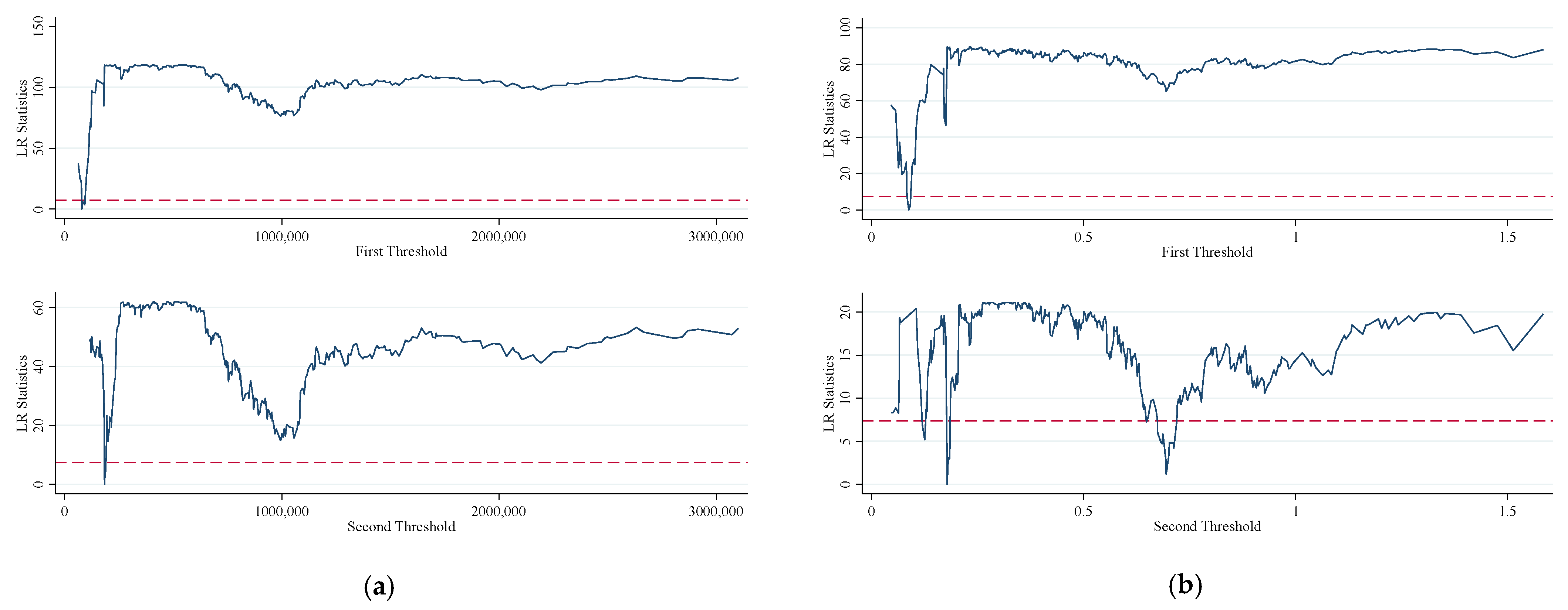
4.2.1. Threshold Effects Test

Since the impact of highway improvements on the URIG remains largely unchanged after accounting for long-term effects and spatial spillover effects compared to the benchmark regression, this study will primarily analyze the threshold effects based on the benchmark regression. Before conducting threshold analysis, two tests are necessary: the first is an existence test for threshold effects, which examines whether parameters in different intervals divided by the threshold are significantly different. The second is a consistency test to compare the estimated and actual values of the threshold variables.

(1) Existence test:

Table 4. Existence test.

	Number	F-Value	1%	5%	10%	p-Value
TGRP	Single	91.79	29.9980	23.4547	19.6903	0.0000
	Double	62.67	25.0396	20.8232	18.4226	0.0000
	Triple	35.62	90.1938	71.4627	60.7924	0.5233
PGRP	Single	75.99	29.2185	22.9179	20.0357	0.0000
	Double	21.35	35.7026	23.9630	20.1957	0.0767
	Triple	17.34	63.1126	42.0299	36.8646	0.5467

Note: p-values are obtained by sampling 300 times using the bootstrap method.

presents the results using TGRP and PGRP as threshold variables. First, single-threshold tests are performed, yielding F-values of 91.79 and 75.99, with p-values of 0.0000, indicating that threshold effects exist regarding the impact of highway improvements on the URIG. Next, double-threshold tests are conducted, resulting in F-values of 62.67 and 21.35, with p-values of 0.0000 and 0.0767, respectively. Both tests reject the null hypotheses of single-threshold effects, confirming the existence of double-threshold effects. Finally, triple-threshold tests are carried out, but the p-values fail to reject the null hypotheses of the double-threshold effects. Therefore, the double-threshold models are selected. As shown in

Table 5. Thresholds and confidence intervals.

	Order	Threshold Value	95% Confidence Interval
TGRP	First (i.e., TLR1)	793.12 (CNY million)	(771.65, 837.22)
	Second (i.e., TLR2)	1836.00 (CNY million)	(1816.98, 1857.00)
PGRP	First (i.e., PLR1)	0.0878	(0.0836, 0.0913)
	Second (i.e., PLR2)	0.1790	(0.1271, 0.1810)

, the first threshold for TGRP (TLR1) is CNY 793.12 million, and the second threshold (TLR2) is CNY 1836.00 million. For PGRP, the first (PLR1) is 0.0878, and the second (PLR2) is 0.1790.

(2) Consistency test: Due to the highly non-standard asymptotic distribution caused by confounding parameters, the existence test alone cannot confirm whether the threshold estimate $\gamma$ is consistent with the actual value ${\gamma }_0$. Therefore, Hansen (1999) proposed using maximum likelihood estimation to derive the asymptotic distribution of the statistic, which can then be used to test the consistency of the estimate with the actual threshold value. The likelihood ratio (LR) function is illustrated in Figure 3. In particular, the horizontal axis of Figure 3a represents the threshold value of TGRP, while the vertical axis represents the LR statistics. The dotted line indicates the critical value at the 95% confidence level. The upper half of the figure corresponds to TLR1, and the lower half corresponds to TLR2. According to Hansen’s LR test formula, the null hypothesis is rejected when $R\left(\gamma \right)>c\left(\theta \right)$. When $\theta =5\%$, the LR statistics for TLR1 and TLR2 are significantly smaller than the critical value, confirming that TLR1 and TLR2 are accurate and valid. Similarly, Figure 3b shows that PLR1 and PLR2 are accurate and valid.

4.2.2. Overall Results

Table 6. Threshold effect results.

	URIG
	Model 1	Model 2
Density (TGRP < TLR1; PGRP < PLR1)	14.2610 ***	10.9056 ***
	(2.1727)	(2.2307)
Density (TLR1 ≤ TGRP < TLR2; PLR1 ≤ PGRP < PLR2)	2.3121 ***	1.5104
	(0.8254)	(1.1186)
Density (TGRP ≥ TLR2; PGRP ≥ PLR2)	−0.7214 **	−0.5823 *
	(0.3201)	(0.3265)
Control variables	YES	YES
County FE	YES	YES
Year FE	YES	YES
Constant	10.6047 ***	8.9891 ***
	(3.2694)	(3.5306)
Observations	1136	1136
R-squared	0.8224	0.8142
F statistic	200.8200	189.7500

Note: (i) In model 1, the threshold variable is TGRP; in model 2, the threshold variable is PGRP. (ii) TLR1 = CNY 793.12 million, TLR2 = CNY 1836.00 million; PLR1 = 0.0878, PLR2 = 0.1790. (iii) The control variables are consistent with those in Table 2, except for the exclusion of GRP, which is omitted based on the rationale of the threshold model. The same applies to the latter. (iv) *, **, *** significant at 10%, 5%, and 1% levels; parentheses indicate robust standard errors.

presents the results of the threshold model, revealing that the relationship between highway improvements and the URIG in underdeveloped regions is divided into three distinct intervals, with significant differences across these intervals. Using TGRP as an example, when TGRP < TLR1, the impact of total highway density on the per capita disposable income ratio between urban and rural residents is significantly positive at the 1% significance level, with an impact coefficient as high as 14.2610. This suggests that at this stage, highway improvements significantly widen the URIG, with most benefits accruing to urban residents, leaving rural residents with little to no share in the gains. When TLR1 ≤ TGRP < TLR2, highway improvements continue to widen the URIG, although the magnitude of the impact decreases substantially. At this stage, rural residents begin to enjoy some benefits, but the majority still goes to urban residents. Once TGRP ≥ TLR2, the impact of total highway density on the income ratio becomes significantly negative at the 5% significance level, indicating that highway improvements can then help narrow the URIG and foster shared prosperity. The results using PGRP as the threshold variable are consistent with those using TGRP, confirming that regional economic development levels play a critical threshold role in how highway improvements affect the URIG. These findings support Hypothesis 1.

Furthermore, to assess the positioning of different threshold values within the overall sample, a probability distribution table of the threshold variables for 2020 is constructed.

Table 7. Distribution of threshold variables in 2020.

	5%	10%	25%	50%	75%	90%	95%
TGRP	1902.98	2848.05	5543.92	8677.61	15,407.29	24,054.81	29,103.42
PGRP	0.1324	0.2141	0.3675	0.5763	0.8693	1.1584	1.3338

shows that TLR2 falls within the low range of less than 5%, while PLR2 falls below 10%. This indicates that after the end of the Targeted Poverty Alleviation Strategy, most counties in underdeveloped regions have already surpassed the second threshold. As a result, these counties have entered a favorable phase where highway improvements have helped narrow the URIG and promote shared prosperity.

4.2.3. Results for Different Highways

Table 8. Threshold effect results for inter-regional highway and county highway.

	URIG
	Model 1	Model 2	Model 3	Model 4
Density_I (TGRP < TLR1_I; PGRP < PLR1_I)	34.3493 ***	21.2736 ***
	(6.2771)	(4.2956)
Density_I (TLR1_I ≤ TGRP < TLR2_I; PGRP ≥ PLR1_I)	6.4016 ***	0.3926
	(1.7163)	(0.6557)
Density_I (TGRP ≥ TLR2_I)	0.0274
	(0.6289)
Density_C (TGRP < TLR1_C; PGRP < PLR1_C)			13.3697 ***	9.4921 ***
			(2.0787)	(1.6358)
Density_C (TLR1_C ≤ TGRP < TLR2; PGRP ≥ PLR1_C)			2.5305 ***	−0.5784 **
			(0.9329)	(0.2644)
Density_C (TGRP ≥ TLR2_C)			−0.7302 ***
			(0.2500)
Control variables	YES	YES	YES	YES
County FE	YES	YES	YES	YES
Year FE	YES	YES	YES	YES
Constant	11.3369 ***	9.7444 ***	10.0421 ***	9.3757 ***
	(3.5430)	(4.2956)	(3.1807)	(3.2982)
Observations	1136	1136	1136	1136
R-squared	0.8208	0.8106	0.8195	0.8091
F statistic	193.7400	194.0500	194.6700	201.7600

Note: (i) In models 1 and 3, the threshold variable is TGRP; in models 2 and 4, the threshold variable is PGRP. (ii) TLR1_I = CNY 793.12 million, TLR2_I = CNY 1864.72 million, PLR1_I = 0.0878; TLR1_C = 79,312, TLR2_C = CNY 1836.00 million, PLR1_C = 0.0720. (iii) ** and *** significant at 5%, and 1% levels; parentheses indicate robust standard errors.

presents further results for inter- and intra-regional highways. Still using TGRP as an example (the results using PGRP as the threshold variable differ from those using TGRP in terms of the number of thresholds, but the overall mode of influence remains similar. For inter-regional highways, the p-value for the F-statistic in the double-threshold significance test is 1.0000, indicating the existence of only a single-threshold effect, with a threshold value (PLR1_I) of 0.0878. When PGRP < PLR1_I, improvements in inter-regional highways tend to widen the URIG. Once TGRP ≥ PLR1_I, the widening effect disappears. For intra-regional highways, the p-value for the F-statistic in the double-threshold significance test is 0.1133, also confirming a single-threshold effect, with a threshold value (PLR1_C) of 0.0720. When PGRP < PLR1_C, county highway improvements widen the URIG. Conversely, when PGRP ≥ PLR1_C, county highway improvements help narrow the URIG.), for inter-regional highways, the p-value for the F-statistic in the double-threshold significance test is 0.0000, confirming the existence of a double-threshold effect. The first threshold (TLR1_I) is CNY 793.12 million, and the second (TLR2_I) is CNY 1864.72 million, closely aligned with the results from the overall regression. As TGRP moves from TLR1_I to TLR2_I, the widening effect of inter-regional highway improvements on the URIG persists, but the impact magnitude significantly decreases. Once TGRP ≥ TLR2_I, this widening effect disappears. For intra-regional highways, the p-value for the F-statistic in the double-threshold significance test is 0.0067, again confirming a double-threshold effect. The first threshold (TLR1_C) is CNY 793.12 million, and the second (TLR2_C) is CNY 1836.00 million, consistent with the overall regression results. As TGRP moves from TLR1_C to TLR2_C, county highway improvements continue to widen the URIG, but the impact is considerably smaller than that of inter-regional highways. Once TGRP ≥ TLR2_C, county highway improvements begin to narrow the URIG.

This finding slightly differs from the benchmark regression, as the threshold effect of regional economic development levels becomes apparent. Nonetheless, both the benchmark and threshold regressions confirm that county highways are the primary factor in reducing the URIG, whereas inter-regional highways have a limited impact. This difference is attributed to the distinct functions of highways at different classes, further supporting Hypothesis 3.

4.3. Robustness Tests

4.3.1. Tests for Threshold Values

The inclusion of control variables may affect the threshold value, so this study tests the robustness of the threshold by gradually incorporating additional control variables. According to the benchmark regression results in Table 2, certain control variables, such as policy support, significantly impact the URIG. Therefore, this study uses policy support as the baseline control variable and progressively adds other control variables in reverse order, with the estimation results shown in

Table 9. Robustness tests for thresholds.

Control Variables	TGRP as Threshold Variable			PGRP as Threshold Variable
	p-Value	TLR1	TLR2	p-Value	PLR1	PLR2
Policy support	0.0000	793.12	1864.72	0.0000	0.0635	0.1089
Policy support + Education, healthcare, and welfare + Fiscal revenues and expenditures	0.0000	793.12	1836.00	0.0000	0.0878	0.1790
Policy support + Education, healthcare, and welfare + Fiscal revenues and expenditures + Residents’ savings + County size	0.0000	793.12	1836.00	0.0000	0.0878	0.1790

Note: (i) TLR1 = CNY 793.12 million, TLR2 = CNY 1836.00 million; PLR1 = 0.0878, PLR2 = 0.1790. (ii) p-values are obtained by sampling 300 times using the bootstrap method.

. When considering only policy support, TLR1 is CNY 793.12 million and TLR2 is CNY 1864.72 million, while PLR1 is 0.0635 and PLR2 is 0.1089. When education, healthcare and welfare, and fiscal revenue and expenditure are added, TLR1 remains at CNY 793.12 million, TLR2 adjusts to CNY 1836.00 million, PLR1 increases to 0.0878, and PLR2 to 0.1790. When residents’ savings and county size are further included, the threshold values remain consistent with the previous step. These results demonstrate that the threshold effect of regional economic development levels on the URIG is robust. Additionally, the threshold values remain stable and are not significantly influenced by including control variables.

4.3.2. Results of the IV Approach

The instrumental variable (IV) is conducted considering several aspects. Firstly, this study utilizes the relief degree of land surface (RDLS) to construct an IV. RDLS influences the complexity and cost of highway construction, but it is unaffected by socio-economic factors, making it inherently exogenous. Similarly, the distance between the county and the capital city is also used to build the IV. Since capital cities are typically regional centers and play a significant role in highway planning, counties closer to them tend to have higher highway densities, and spatial distance is strictly exogenous. However, RDLS and spatial distance cannot be used as IVs in panel data analysis because they do not vary over time. To address this, a time-varying exogenous variable is introduced [49,50], namely the total population of the county [51]. Larger populations generate greater demand for highways, which is linked to higher highway densities. However, the total population is relatively exogenous to the URIG, as it is unlikely to influence the URIG directly. Therefore, the product of RDLS, spatial distance, and total population varies across both cross-sectional and temporal dimensions, making it a suitable IV for highway improvement.

Table 10. Results of the IV approach.

	URIG
	Model 1: All		Model 2: TGRP > TLR2		Model 3: PGRP > PLR2
	Step 1	Step 2	Step 1	Step 2	Step 1	Step 2
IV	−0.0151 ***		−0.0167 ***		−0.0179 ***
	(0.0029)		(0.0029)		(0.0029)
Density		−1.5796		−2.3347 *		−3.3394 ***
		(1.6465)		(1.4095)		(1.3911)
Control variables	YES	YES	YES	YES	YES	YES
County FE	YES	YES	YES	YES	YES	YES
Year FE	YES	YES	YES	YES	YES	YES
Observations	1136	1136	1000	1000	984	984
F statistic	27.4100	199.2100	34.2400	179.7900	39.0700	178.3300
Kleibergen-Paap rk LM statistic	16.0160 ***		18.1580 ***		18.3010 ***
Cragg-Donald Wald F statistic	25.1370 ***		29.4570 ***		31.1370 ***
Kleibergen-Paap rk Wald F statistic	27.4110 ***		34.2400 ***		39.0660 ***
Hansen J statistic	0.0000		0.0000		0.0000

Note: (i) TLR2 = CNY 1836.00 million, PLR2 = 0.1790. (ii) * and *** significant at 10% and 1% levels; parentheses indicate robust standard errors.

presents the results using the IV approach, with model 1 presenting the full-sample estimates and model 2 and model 3 presenting the results of the sub-sample estimates that lie to the right of TLR2 and PLR2, respectively. Firstly, in terms of the validity, Kleibergen–Paap rk LM statistics are significant, firmly rejecting the null hypotheses of underidentification. The Cragg–Donald Wald F statistics and Kleibergen–Paap rk Wald F statistics exceed Stock–Yogo’s critical value of 16.38, confirming that weak instrumental variables are not an issue. Thus, the IVs selected in this study are valid and appropriate. Secondly, the results show that highway improvement does not have a significant effect on the URIG in the full sample but significantly reduces the URIG when the TGRP and PGRP are higher than TLR2 and PLR2, which is in line with the previous results.

4.3.3. Separating the Impact of the ORDP

To assess the impact of other regional policies, this study considers the Old Revolutionary Development Program (ORDP), a key national effort. The ORDP targets former revolutionary base areas during the Second Domestic Revolutionary War and the Anti-Japanese War, covering 1599 counties. Since 2012, five rounds of ORDPs have been approved by the State Council, providing substantial support. To separate the ORDP’s influence, this study incorporates an “ORDP” variable, assigning a value of “1” to counties included in the program for the relevant year and “0” to those not covered. Even after accounting for the ORDP, regional economic development levels maintain a consistent double-threshold effect (

Table 11. Results of robustness tests.

	URIG
	ORDP	CTR	HSR	Character	Weight
	Model 1	Model 2	Model 3	Model 4	Model 5
Density (TGRP < TLR1)	14.5621 ***	14.2998 ***	14.1771 ***	15.1551 ***	16.7455 ***
	(2.2492)	(2.1721)	(2.1663)	(2.1030)	(2.6733)
Density (TLR1 ≤ TGRP < TLR2)	2.5326 ***	2.3187 ***	2.2203 ***	2.2795 ***	2.7434 ***
	(0.8197)	(0.8246)	(0.8323)	(0.8402)	(0.9420)
Density (TGRP ≥ TLR2)	−0.5461 *	−0.7245 **	−0.7517 **	−0.6886 **	−0.7064 *
	(0.3167)	(0.3185)	(0.3194)	(0.3313)	(0.3931)
ORDP	−0.1250 ***
	(0.0374)
CTR		−0.1514 *
		(0.0889)
HSR			0.0410
			(0.0363)
Control variables	YES	YES	YES	YES	YES
County FE	YES	YES	YES	YES	YES
Year FE	YES	YES	YES	YES	YES
Constant	9.7458 ***	10.5715 ***	10.4036 ***	10.1774 ***	10.7103 ***
	(3.1472)	(3.2670)	(3.2894)	(3.3036)	(3.3301)
Observations	1136	1136	1136	1136	1136
R-squared	0.8260	0.8235	0.8228	0.8339	0.8221
F statistic	189.1300	187.2800	187.9800	206.7900	200.4000

Note: (i) In model 1, TLR1 = CNY 793.12 million, TLR2 = CNY 1836.00 million; in model 2, TLR1 = CNY 793.12 million, TLR2 = CNY 1836.00 million; in model 3, TLR1 = CNY 793.12 million, TLR2 = CNY 1836.00 million; in model 4, TLR1 = CNY 787 million, TLR2 = CNY 1877.96 million; in model 5, TLR1 = CNY 793.12 million, TLR2 = CNY 1836.00 million. (ii) *, **, *** significant at 10%, 5%, and 1% levels; parentheses indicate robust standard errors.

, model 1).

4.3.4. Separating the Impact of Railway Development

Besides highways, China’s “transportation power” strategy has also spurred vast development in railways. This study adds specific variables to the threshold regression model to account for the potential effects of railway development. The variable “CTR” is set to “1” if a conventional railway line traverses the county in the relevant year and “0” if it does not; “HSR” is similarly defined for high-speed railways. After adjusting for the presence of railway development, the double-threshold effect persists and threshold values remain consistent (Table 11, models 2 and 3).

4.3.5. Separating the Impact of County Characteristics

Considering potential reverse causality between highway improvements and the URIG at the county level, even though county governments typically do not have discretionary power or sufficient funding for highway construction, this study also adopts the “non-critical city” approach suggested by existing research [52] for this issue. In China, “county-level cities”, “city districts”, and “special zones” generally hold advantages over standard counties. Following this, the sample is limited to “counties” and “autonomous counties” only. The findings remain robust after this adjustment (Table 11, model 4).

4.3.6. Substituting Core Explanatory Variable

Since travel time is typically the primary focus of attention, speed is used as the weighting factor. However, highway grading also encompasses other factors, such as traffic load and construction limits. Among these, the traffic load across different highways varies significantly, affecting the actual capacity. Therefore, this study recalculates the core explanatory variable, using traffic load as the weighting factor. According to JTG B01-2014, the designated traffic load for minibusses is above 15,000 vehicles for expressways and national highways, 5000 to 15,000 vehicles for provincial highways, and 2000 to 6000 vehicles for county highways, with respective weights of 1.36, 1.36, 0.91, and 0.37. As a result, the total highway density is formulated as total highway density = 1.36 × expressway density + 1.36 × national highway density + 0.91 × provincial highway density + 0.37 × county highway density. The findings remain robust after this adjustment (Table 11, model 5).

4.4. Heterogeneity Analysis

Highway improvements act as an external shock, and their effect on residents’ income may be constrained by various factors in the regional environment surrounding residents, from their initial occurrence to eventual transmission. The threshold effect of the regional economic development levels may differ as a result, necessitating an analysis of heterogeneity. This study primarily analyzes the development belt in which the county is situated and the county’s industrial structure. The former is used to examine the impact of the indirect environment surrounding residents, while the latter focuses on the direct environment.

4.4.1. Under Different Regional Development Belt

In order to optimize resource allocation and promote coordinated development, China has divided several regional development belts within which regions share resources and develop synergistically. Among these, the Yangtze River Economic Belt, centered around the Yangtze River, covers multiple provinces and is one of the most economically dynamic regional development belts. As such, this study takes the Yangtze River Economic Belt as a representative of the regional development belt. A value of “1” is assigned when a county is part of this belt and “0” otherwise, with the results presented in

Table 12. Results of heterogeneity analysis.

	Belt		Structure
	Yes	No	Advanced	Backward
	Model 1	Model 2	Model 3	Model 4
Density (TGRP < TLR1)	14.5680 ***	10.8130 ***	13.5583 ***	20.7037 ***
	(3.2413)	(2.8417)	(2.2958)	(4.4770)
Density (TLR1 ≤ TGRP < TLR2)	−1.5360 ***	1.5669	2.1487 **	−0.3823
	(0.4180)	(1.2122)	(1.0481)	(0.4273)
Density (TGRP ≥ TLR2)	−0.5126	−0.8716	−1.1436 **
	(0.4063)	(0.6562)	(0.4892)
Control variables	YES	YES	YES	YES
County FE	YES	YES	YES	YES
Year FE	YES	YES	YES	YES
Constant	12.8523	11.7550 ***	9.4681 **	12.3007 **
	(8.3723)	(2.9748)	(4.4517)	(4.8445)
Observations	648	488	382	754
R-squared	0.8228	0.8583	0.8710	0.8018
F statistic	139.9600	108.6100	110.1000	132.9200

Note: (i) In model 1, TLR1 = CNY 1199.32 million, TLR2 = CNY 8699.40 million; in model 2, TLR1 = CNY 793.12 million, TLR2 = CNY 1885.47 million; in model 3, TLR1 = CNY 793.12 million, TLR2 = CNY 1835.85 million; in model 4, TLR1 = CNY 1295.00 million. (ii) ** and *** significant at 10% and 1% levels; parentheses indicate robust standard errors.

. The double-threshold effect of regional economic development levels exists regardless of whether a county is part of the belt or not. However, when a county is located within this belt, highway improvements can help narrow the URIG once regional economic development levels cross the threshold (model 1). Conversely, in counties outside the belt, highway improvements do not lead to such results (model 2). This discrepancy may be due to the close interactions within the belt. In counties within the belt, highway improvements can facilitate the entry of enterprises from more developed regions, boosting local employment. Additionally, rural residents in these counties can migrate to developed regions for work more easily. Conversely, counties outside the belt lack these opportunities. Even if their regional economic development levels surpass the threshold, highway improvements do not offer substantial income-boosting opportunities for rural residents, thus failing to narrow the URIG.

4.4.2. Under Different Industrial Structure

Industrial structure plays a crucial role in shaping employment patterns, which in turn affects the opportunities available to rural residents. Industrial structure is measured by the ratio of the value of the tertiary industry to the secondary industry in the initial year. A higher ratio indicates a more advanced industrial structure. The results, as shown in Table 12, are based on the mean value as the cutoff point. The threshold effect of regional economic development levels is evident in both cases. However, it is only in regions with an advanced industrial structure that highway improvements can reduce the URIG once regional economic development levels cross the threshold (models 3 and 4). In regions with a backward industrial structure, even if the regional economic development levels surpass the threshold, highway improvements mainly promote the growth of industries with limited employment capacity, making it difficult to generate sufficient job opportunities for rural residents. However, as the share of tertiary industries rises, highway improvements can encourage the development of similar industries with greater employment potential, thereby creating more job opportunities and helping to narrow the URIG.

5. Further Analysis

The results of the quantitative analysis confirm the presence of a threshold effect in regional economic development levels when reducing the URIG through highway improvements. This section delves into the underlying reasons for this threshold effect through qualitative analysis, utilizing first-hand case data obtained from field surveys conducted in Lankao County and Rongjiang County.

5.1. Differences in Local Non-Farm Employment: Different Participation Opportunities

5.1.1. Situation in Lankao County

Benefiting from its strategic location within the Kaifeng, Heze, and Shangqiu triangle, Lankao County has a strong advantage in attracting investment. Since officially entering the poverty alleviation stage in 2012, the county has developed a relatively distinctive industrial system within four years, encompassing green animal husbandry, intelligent manufacturing, and so on. As a result, Lankao County leads in regional economic development levels among poverty-alleviated counties and has gradually established a development foundation that could benefit the deepening of its industrial structure. Later, with the creation of the “seven vertical and seven horizontal”, Lankao’s home furnishing industry was able to develop further, playing a crucial role in narrowing the URIG.

Specifically, Lankao County has developed a comprehensive home furnishing industry chain encompassing core manufacturing, wood product processing, and forestry planting. With improvements in inter-regional transportation, the region’s accessibility has significantly increased. Building on the development foundation, Evergrande Group set up operations in the Modern Home Furnishing Industrial Park located in the county seat in 2018. Following Evergrande, over 40 home furnishing enterprises also established operations in the park. By 2021, the park covered approximately 13,000 acres, creating more than 2400 jobs. These newly created positions added to the existing jobs in former industries, generating a broad labor market within the county. This expansion not only provided employment opportunities for county-seat laborers but also absorbed rural laborers (see 2023LK-RRB01). Additionally, the relatively lower cost of rural labor has made these laborers attractive to enterprises, allowing rural laborers to access more opportunities for local non-farm employment.

“Lankao is unique because many laborers work within the county itself. With ample job opportunities, farmers prefer commuting to town from remote villages since the roads to the county seat are good. Every day around 6 p.m., when the industrial zone closes, people hop on buses or ride their electric scooters straight home.”

(2023LK-RRB01)

Furthermore, as non-agricultural industries concentrate in the county seat, rising land prices and wages have driven parts of the industrial chain to relocate to townships and rural areas. High-quality intra-regional highways have facilitated this shift, enabling Lankao to establish a new urban–rural industrial layout. In the wood product processing sector, Lankao County has developed six specialized township industrial parks, following the principle of “one industry for one township”, housing over 2000 supporting enterprises. In the forestry planting sector, raw materials such as paulownia, poplar, and willow are all cultivated in rural areas. Expanding non-agricultural industries into townships and rural areas has created more employment opportunities “at the doorstep” for rural laborers. This not only contributes directly to increasing wage incomes but also provides a fallback option for those who may not succeed in migrant non-farm employment or agricultural operations, ensuring they have the means to maintain income growth (see 2023LK-FCC03, 2023LK-ZZC04). By 2021, the home furnishing industry had developed into a robust industrial system employing over 100,000 people, accounting for approximately 11% of the county’s total workforce. Annual per capita income in this industry ranged from CNY 80,000 to 100,000, significantly contributing to the narrowing of the URIG.

“Wood door manufacturing requires a full-time workforce year-round for tasks like fine cutting, sanding, milling, and spraying, which drives up labor costs—especially in the county seat. In our village, labor costs are lower, and being close to the X052 highway makes transportation easier. That’s why we set up a wood-products processing industrial park here.”

(2023LK-QLGC01)

“I learned piano-making from my father, but before that, I did various labor jobs elsewhere. I started working at this factory in 2018. The monthly pay isn’t bad—over 6000 yuan in a good month. Plus, it’s close to home, so I can care for my family.”

(2023LK-FCC03)

“I must care for my family and children, so I can’t work elsewhere. This village company has helped solve employment issues for women like me who stay behind. We’re paid by the piece, so the more we work, the more we earn—about 4000 yuan a month.”

(2023LK-ZZC04)

5.1.2. Situation in Rongjiang County

Unlike Lankao County, Rongjiang County, situated in a mountainous region, lacks geographical advantages to attract investment. Until 2020, Rongjiang remained a traditional agricultural county with non-agricultural industries limited to primary wood processing. The regional economic development level was significantly underdeveloped, lacking the development foundation needed for the deepened development of non-agricultural industries. Later, the opening of key transportation routes, such as the Guiguang High-Speed Railway in 2015, the Jianrong Expressway in 2021, and the Leirong Expressway in 2023, provided new opportunities for non-agricultural industry growth, but the county continues to face challenges in reducing the URIG.

In the secondary industry, Rongjiang Industrial Park, located on the east side of the county seat, was initially built around the southern Xiarong Expressway and later benefited from additional routes. The park has attracted several companies. However, underdeveloped economic conditions have limited the county’s capacity to support the scaling and diversification of the secondary industry, which remains centered on an OEM-based primary wood processing industry and offers only limited non-farm employment opportunities. In the tertiary industry, the success of the “Village Super” tournament in 2023 has increased tourism output in Rongjiang County, but the industry is still in its early stages and cannot generate many permanent jobs. Overall, the region’s low economic development levels mean that the limited number of non-farm jobs created by highway improvements are quickly absorbed into an already small non-farm job market. Rural laborers face challenges in accessing these participation opportunities, as urban workers, who enjoy a “first-mover advantage”, dominate the non-farm job market (see 2024RJ-RRB02). This situation restricts the potential for highway improvements to effectively reduce the URIG in Rongjiang County.

“There are only so many jobs in the county seat, and even people there struggle to find work, let alone farmers. Some might build a wooden house or have enough business sense to sell some trees, but wages are low—maybe two or three thousand yuan for hard labor.”

(2024RJ-RRB02)

Furthermore, unlike Lankao County, the development of non-agricultural industries within Rongjiang County’s seat has not yet reached a saturation point and therefore lacks the incentive for industrial transfer. Moreover, rural areas lack the necessary prerequisites to support the transfer of non-agricultural industries (see 2024RJ-RRB01). For the secondary industry, traditional agriculture has long dominated the rural economy, preventing the establishment of essential conditions—such as available land, skilled labor, and technological support—for secondary industry development. For the tertiary industry, although rural areas are known for their scenic landscapes, the necessary foundation for tourism is underdeveloped. In addition, the steep valleys create winding roads that pose challenges for large transport vehicles and public buses accessing rural areas, leading to high trade and mobility costs.

“There’s no wood processing industry in the village because transportation costs are too high, and there’s no supporting industrial chain. If an industrial chain is established in the future, it might be possible, but it will require time and a solid foundation. As for tourism, few villages can develop it. Out of our 250 villages, maybe 15 are involved in tourism. The rest rely mainly on aging industries, and the issue of village hollowing is severe.”

(2024RJ-RRB01)

More importantly, the lack of local non-farm job opportunities has created two significant challenges that severely hinder efforts to reduce the URIG. In the short term, some rural laborers cannot leave their hometowns due to caregiving responsibilities, such as caring for elderly family members or supporting their children’s education. In the long term, laborers who initially seek jobs outside may be forced to return for various reasons, such as aging, health issues, or restrictions on access to education in urban areas. A key factor in this situation is the inequality in educational opportunities between migrant and local children tied to the hukou system. Although reforms have improved the educational rights of migrant children during compulsory education, a significant gap remains at the high school level (by 2020, substantial progress had been achieved in promoting educational equity for migrant children in compulsory education. A total of 14.297 million migrant children were enrolled in compulsory education, with 85.8% attending public schools or receiving government-sponsored education services. However, data from the China Family Panel Studies (CFPS) show that in 2020, only 57.41% of children aged 16 to 18 who migrated with their families were enrolled in high school education compared to the national average of 71.99%, revealing a gap of 14.58 percentage points. This disparity underscores the ongoing inequality in access to high school education for children from migrant families). Many rural families, unable to meet the high school entrance requirements in urban areas, are forced to either keep a laborer at home or have some laborers return home to accompany their children. Despite highway improvements, the limited availability of non-farm jobs due to the region’s low economic development levels means that these laborers face few employment opportunities. Most of them work in low-wage service sectors or are forced to withdraw from the paid labor market altogether (see 2024RJ-DJC02, 2024RJ-LXC02, 2024RJ-JYC03).

“I wanted to work outside, but at the time, I had a young child and elderly family members to care for. If I had gone, I’d probably be much better off now, maybe 5000 yuan a month. There aren’t factories nearby, so I opened this small restaurant, less than 2000 yuan a month.”

(2024RJ-DJC02)

“We worked outside until 2014, but when our child had to return for school, we returned and started a small business. Running a shop isn’t as profitable as it used to be, and the profit margins are slim—not nearly as good as what we could earn working outside.”

(2024RJ-LXC02)

“I worked outside when I was younger, but as I got older and developed a chronic illness, factories didn’t want to hire me. There’s not much money to be made around here. I watch over the forest as a public service job, earning 800 yuan a month.”

(2024RJ-JYC03)

5.2. Differences in Migrant Non-Farm Employment: Different Wage Returns

5.2.1. Situation in Lankao County

As previously mentioned, rural laborers, due to generally lower levels of education and skills, often face limited employment options in large cities. In response, Lankao County has increased its investment in education for both urban and rural residents, utilizing sufficient funds and abundant resources. Special preference has been given to disadvantaged groups in rural areas.

In 2022, Lankao County launched a government-funded program aimed at upgrading the skills of working-age laborers through various vocational training initiatives. The first initiative focused on skills enhancement for stable employment, with government financial support as its foundation. Technical schools and skill training institutions played a central role, targeting disadvantaged groups such as rural migrant workers, retired military personnel, people with disabilities, and zero-employment families. Through this program, 28,951 individuals received vocational training, resulting in 11,779 newly skilled laborers. The second initiative centered on expanding local specialty brands by capitalizing on the county’s unique ethnic musical instrument resources. This led to the training of 663 ethnic stringed instrument makers and 756 ethnic plucked instrument makers. Additionally, to foster long-term human capital development, Lankao County implemented targeted financial assistance policies for students at all educational levels. In 2022, 60,978 students received financial assistance, totaling CNY 51.15 million. Notably, the majority of these students came from previously impoverished households, and the financial support provided to them far exceeded that given to children from non-impoverished families (for example, at the high school education level, students from low-income families in Lankao County who are household members and attend full-time high schools within the county receive a living allowance of CNY 5000 per student per year. In contrast, ordinary students who are household members and attend full-time high schools within the county receive a living allowance of CNY 1000 per student per year).

As a result, counties with relatively higher economic development levels, such as Lankao County, which have access to abundant financial resources, can invest more in the education of rural residents. This investment produces a rural labor force with relatively higher human capital levels. Once highway improvements reduce transfer costs, these rural laborers can pursue jobs that better match their skills, enabling them to secure higher wage returns (see 2023LK-ZZC01, 2023LK-DZC02), thereby further narrowing the URIG.

“We have Sannong Vocational College and the Higher Technical School, and many people from our village studied there. Two main groups now earn excellent salaries—those who repair boilers for companies and those working in engineering in Xinjiang. They’re making seven to eight thousand yuan a month now.”

(2023LK-ZZC01)

“Experts taught us cultivation techniques for these key honeydew melons, and the county invested significantly to bring them in. Experts also visit the fields daily. My partner has become a technician and often travels for months, providing technical guidance in other places and earning a good income. Just a few days ago, he went to Shangqiu for this purpose.”

(2023LK-DZC02)

5.2.2. Situation in Rongjiang County

As previously analyzed, highway improvements in Rongjiang County have not effectively stimulated the development of non-agricultural industries. Instead, these improvements primarily facilitate the migration of rural laborers. Consequently, migrant employment in Rongjiang County plays a more significant role in influencing the URIG, as it constitutes a substantial proportion of non-farm employment. Although the government prioritizes enhancing human capital for both urban and rural residents, efforts to train rural laborers are limited by constrained local financial resources and funding.

For vocational skills training, Rongjiang County adopts a more flexible “bottom-up” approach in contrast to the government-led “top-down” strategy in Lankao County. Training programs are tailored to the specific development needs and requests of certain areas, with relevant support units providing short-term targeted training. For instance, the State Railway Administration conducted 7-day masonry skills training at the Chemin Street resettlement site, attended by 52 laborers. Additionally, the Guangdong–Guizhou Collaboration Welding Customized Class was held at the County Secondary Vocational School for 36 days with 56 participants. Although this decentralized approach addresses specific needs, the lack of unified government support results in limited content scope and reach, making it challenging to meet the broader training demands of the larger migrant labor population. Rongjiang County also emphasizes long-term human capital development and educational investment. In 2022, the county allocated CNY 27.91 million in financial aid to support 47,406 students from economically disadvantaged families. Compared to Lankao County, it faces greater pressure regarding the total number of students supported, with 12.31% of its population receiving aid compared to Lankao’s 7.05%. However, due to financial constraints, per capita funding in Rongjiang County is significantly lower, at CNY 588.79 compared to Lankao’s CNY 838.85.

As a result, counties with relatively low economic development levels, such as Rongjiang County, lack sufficient funds and resources to invest adequately in education for rural residents. This leads to lower human capital levels among rural laborers, many of whom end up in low-skill industries in large cities, relying on physical labor to earn an income. A village secretary in Rongjiang County remarked to rural laborers, “The biggest resource farmers have is their physical strength, which ultimately overdraws their bodies.”. Rural residents’ low wages in such physically demanding low-skill jobs do little to reduce the URIG (see 2024RJ-JYC02, 2024RJ-THSQ03).

“My two sons and daughter-in-law work in Jieyang, cutting wood in the mountains. They earn about 4000 yuan a month. It’s not much, but without skills, we must rely on physical labor to make a living.”

(2024RJ-JYC02)

“Both of my sons work in Dongguan. The older one is in a garment factory, and the younger one works in a toy factory. They’re both on the assembly line, earning less than 5000 yuan a month. The eldest started working after three years of vocational school, and the youngest went straight to work after high school. With limited education, it’s hard for them to find better-paying jobs.”

(2024RJ-THSQ03)

5.3. Results Drawn from Comparing the Two Counties

Lankao County and Rongjiang County clearly illustrate the threshold effect of regional economic development levels on how highway improvements influence the URIG.

In terms of local non-farm employment, Lankao County, with its relatively higher regional economic development level, had already established a favorable non-agricultural industry foundation, laying the groundwork for further industrial deepening. Later, highway improvements facilitated the expansion of the home furnishing industry, providing rural laborers with two main avenues for local employment. First, the core manufacturing sector created numerous jobs. Since urban laborers were already employed in existing industries, many of these new positions were filled by rural laborers. Second, as non-agricultural industries in the county seat reached saturation, the wood product processing and forestry planting sectors expanded into rural areas, offering “at-the-doorstep” employment opportunities for rural residents. As a result, rural laborers gained nearly equal access to local employment as their county-seat counterparts. In contrast, Rongjiang County, with its lower regional economic development level, experienced slower growth in non-agricultural industries and lacked the necessary conditions for further industrial development. Although highway improvements spurred initial growth in secondary and tertiary industries, they have not created sufficient employment opportunities for rural laborers. First, the primary wood processing and cultural tourism industries generated only a limited number of jobs. Given the county’s previously scarce employment opportunities, most of these new positions were filled by county-seat laborers, leaving rural laborers behind. Second, the unsaturated non-agricultural industries in the county seat and the lack of an industrial foundation in rural areas hindered the gradient transfer of non-agricultural industries. As a result, rural residents face far fewer local employment opportunities than their county-seat counterparts. When rural laborers are forced to stay or return to their hometowns, they struggle to find suitable employment.

In terms of migrant non-farm employment, while highway improvements may appear to impact labor migration uniformly by reducing mobility costs and increasing employment opportunities, regional economic development levels significantly influence the quality of rural labor migration. In Lankao County, with a higher regional economic development level, the government has sufficient financial resources to invest in both short-term and long-term human capital for rural residents. Consequently, the rural labor force has a relatively higher human capital level. Once highway improvements lower mobility costs, these laborers can leverage their skills to secure better-matched jobs, leading to higher wage returns. In contrast, Rongjiang County, which is economically underdeveloped and lacks financial resources, struggles to provide consistent and adequate investment in human capital for rural residents. As a result, the rural labor force has a lower human capital level. When highway improvements reduce mobility costs, most rural laborers are limited to low-skilled jobs that rely on physical labor, resulting in lower wage returns. Furthermore, the scarcity of local non-farm employment opportunities has made migrant non-farm employment essential for Rongjiang County, but the low wage returns have exacerbated the URIG.

In conclusion, regarding local non-farm employment, regional economic development levels influence the initial scale and foundation of non-agricultural industries, shaping the distribution of subsequent non-farm firms and job opportunities following highway improvements, consequently affecting rural labor participation. Regarding migrant non-farm employment, regional economic development levels determine the intensity of human capital investment for rural residents, impacting rural laborers’ skill levels and, consequently, the wage returns they receive after highway improvements. In summary, regional economic development levels affect both the quantity and quality of rural labor’s transfer to non-farm employment after highway improvements. This ultimately influences the income gap between urban and rural laborers, indicating that highway improvements can either widen or narrow the URIG depending on regional economic development levels. Thus, Hypothesis 2 is confirmed.

6. Conclusions and Policy Implications

This study focuses on national poverty-alleviated counties in central and western China, using a mixed-method approach to examine the non-liner impact of highway improvements on the URIG. The key findings are as follows:

First, analyses using TGRP and PGRP as threshold variables reveal that regional economic development levels exert a double-threshold effect on how highway improvements impact the URIG. When the second thresholds are not reached, highway improvements tend to widen the URIG; once these thresholds are surpassed, highway improvements contribute to narrowing the URIG. Specifically, the second threshold for TGRP is CNY 1836.00 million, and for PGRP, it is 0.1790—both falling below the 10% range in 2020—indicating that in underdeveloped regions, highway improvements have not only boosted absolute income growth but also supported relative income growth. Second, the impact of different highway classes on the URIG varies, reflecting their distinct functions. Inter-regional highways, such as expressways, national highways, and provincial highways, have limited effects on reducing the URIG. Once the relevant thresholds are crossed, their impact shifts from widening the URIG to having no effect. In contrast, county highways (intra-regional highways) play a crucial role in narrowing the URIG. Once the corresponding thresholds are surpassed, improvements in county highways significantly reduce the URIG. Third, the heterogeneity analysis reveals that the impact of highway improvements on the URIG varies depending on the external environment in which residents are situated. This includes both the indirect environment, represented by the development belt the county belongs to, and the direct environment, represented by the county’s industrial structure. Highway improvements can only reduce the URIG when the county is part of a regional development belt or has an advanced industrial structure after the regional economic development level crosses the threshold. Fourth, the qualitative analysis identifies reasons behind the threshold effect of regional economic development levels from the perspective of rural labor transfer to non-farm employment. For local employment, regional economic development levels influence the initial scale and foundation of non-agricultural industries, shaping the distribution of subsequent non-farm firms and job opportunities following highway improvements consequently affecting rural labor participation. For migrant non-farm employment, regional economic development levels determine the intensity of human capital investment for rural residents, impacting rural laborers’ skill levels and, consequently, the wage returns they receive after highway improvements.

The findings provide valuable insights for policymakers to optimize highway planning and reduce the URIG, which will help mitigate inequalities and promote social sustainability. Firstly, the study reveals a non-linear relationship between highway improvements and the URIG in underdeveloped regions, indicating that the income distribution effect of highway improvements alone remains “limited”. To effectively reduce the URIG, highway improvements must be accompanied by complementary measures, with economic growth as the central focus. Meanwhile, a county’s economic growth should be closely aligned with the overall regional development strategy, leveraging structural differences and comparative advantages to facilitate the effective integration of resources and continuous industrial upgrading. Secondly, to fully leverage the labor transfer effects of highway improvements, comprehensive policy support is essential. On the one hand, it is crucial to attract targeted investments to underdeveloped regions by capitalizing on their unique natural resources and low-cost production factors. For instance, encouraging participation in initiatives like the national “One Belt, One Road” program and events like the West China Expo can help secure cooperative projects that align with local strengths. On the other hand, the active implementation of education and talent development policies is needed to raise the educational levels of rural laborers, enabling them to make informed job choices and better adapt to the evolving industrial landscape in larger cities. Lastly, emphasis should be placed on the overall planning of the highway network. Specifically, highway planning should prioritize linking intra-regional highways, such as county highways, with inter-regional highways, creating a cohesive and interconnected network that maximizes the flexibility and functionality of the transport system. Within the county, the intra-regional highway network should be designed to center around county seats, with connections radiating outwards to townships and rural areas.

It is important to note that the thresholds identified in this study, based on TGRP and PGRP, represent only the inflection points in the relationship between highway improvements and the URIG. These thresholds do not signify a dramatic shift in the URIG once each county surpasses them. Therefore, the thresholds reported in this study should not be viewed as fixed values but rather as indicative of significant points where the relationship between highway improvements and the URIG changes. Despite this, the findings still carry important economic and policy implications, as discussed above. A limitation of this study is that it analyzes data in 2012 and 2020, reflecting significant changes in underdeveloped regions during the poverty alleviation stage. While some changes were observed in the data, extending the time frame to capture a longer period would help capture developments during the ongoing stages of rural revitalization and shared prosperity.

References

- Wang, Z.; Zheng, X.; Wang, Y.; Bi, G. A Multidimensional Investigation on Spatiotemporal Characteristics and Influencing Factors of China’s Urban-Rural Income Gap (URIG) since the 21st Century. Cities 2024, 148, 104920. [Google Scholar] [CrossRef]
- Luo, C.; Chen, G. The Plutocrat Lists and Re-estimating Wealth Inequality. China Econ. Q. 2021, 21, 201–222. (In Chinese) [Google Scholar] [CrossRef]
- Chen, D.; Ma, Y. Effect of Industrial Structure on Urban–Rural Income Inequality in China. China Agr. Econ. Rev. 2022, 14, 547–566. [Google Scholar] [CrossRef]
- Quito, B.; Del Río-Rama, M.D.L.C.; Peris-Ortiz, M.; Álvarez-García, J. Spatial-Temporal Determinants of Income Inequality in the Cantons of Ecuador between 2010 and 2019: A Spatial Panel Econometric Analysis. J. Knowl. Econ. 2023, 15, 7744–7768. [Google Scholar] [CrossRef]
- Tang, J.; Gong, J.; Ma, W.; Rahut, D.B. Narrowing Urban–Rural Income Gap in China: The Role of the Targeted Poverty Alleviation Program. Econ. Anal. Policy 2022, 75, 74–90. [Google Scholar] [CrossRef]
- Wang, S.; Tan, S.; Yang, S.; Lin, Q.; Zhang, L. Urban-Biased Land Development Policy and the Urban-Rural Income Gap: Evidence from Hubei Province, China. Land. Use Policy 2019, 87, 104066. [Google Scholar] [CrossRef]
- Ghani, E.; Goswami, A.G.; Kerr, W.R. Highway to Success: The Impact of the Golden Quadrilateral Project for the Location and Performance of Indian Manufacturing. Econ. J. 2016, 126, 317–357. [Google Scholar] [CrossRef]
- Nakamura, S.; Bundervoet, T.; Nuru, M. Rural Roads, Poverty, and Resilience: Evidence from Ethiopia. J. Devel Stud. 2020, 56, 1838–1855. [Google Scholar] [CrossRef]
- Idei, R.; Kato, H. Medical-Purposed Travel Behaviors in Rural Areas in Developing Countries: A Case Study in Rural Cambodia. Transportation 2020, 47, 1415–1438. [Google Scholar] [CrossRef]
- Calderón, C.; Chong, A. Volume and Quality of Infrastructure and the Distribution of Income: An Empirical Investigation. Rev. Income Wealth 2004, 50, 87–106. [Google Scholar] [CrossRef]
- Li, Y.; DaCosta, M.N. Transportation and Income Inequality in China: 1978–2007. Transp. Res. Part. A Policy Pract. 2013, 55, 56–71. [Google Scholar] [CrossRef]
- Jin, M.; Gu, R.; Li, K.X.; Shi, W.; Xiao, Y. Heterogeneous Impacts of the High-Speed Railway Network on Urban–Rural Income Disparity: Spatiotemporal Evidence from Yangtze River Delta of China. Transp. Res. Part. A Policy Pract. 2024, 183, 104050. [Google Scholar] [CrossRef]
- Ren, X.; Zhang, Z. Transportation Infrastructure, Factor Mobility and Urban-Rural Income Gap. Manag. Rev. 2013, 25, 51–59. (In Chinese) [Google Scholar] [CrossRef]
- Jacoby, H.G.; Minten, B. On Measuring the Benefits of Lower Transport Costs. J. Devel Econ. 2009, 89, 28–38. [Google Scholar] [CrossRef]
- Raychaudhuri, A.; De, P. Trade, Infrastructure and Income Inequality in Selected Asian Countries: An Empirical Analysis. In International Trade and International Finance: Explorations of Contemporary Issues; Roy, M., Sinha Roy, S., Eds.; Springer India: New Delhi, India, 2016; pp. 257–278. ISBN 978-81-322-2797-7. [Google Scholar]
- Zhang, Z.; Li, S.; Zhou, J. The Crowding Out Effect of Investment in Public Transport Infrastructure: Perspective of Vulnerability in Residents’ Income Growth. China Soft Sci. 2013, 10, 68–82. (In Chinese) [Google Scholar]
- Adu-Gyamfi, A. Planning for Peri Urbanism: Navigating the Complex Terrain of Transport Services. Land. Use Policy 2020, 92, 104440. [Google Scholar] [CrossRef]
- He, L.; Zhang, X. The Distribution Effect of Urbanization: Theoretical Deduction and Evidence from China. Habitat. Int. 2022, 123, 102544. [Google Scholar] [CrossRef]
- Xia, H.; Yu, H.; Wang, S.; Yang, H. Digital Economy and the Urban–Rural Income Gap: Impact, Mechanisms, and Spatial Heterogeneity. J. Innov. Knowl. 2024, 9, 100505. [Google Scholar] [CrossRef]
- Su, C.; Song, Y.; Ma, Y.; Tao, R. Is Financial Development Narrowing the Urban–Rural Income Gap? A Cross-regional Study of China. Pap. Reg. Sci. 2019, 98, 1779–1801. [Google Scholar] [CrossRef]
- Chen, C.; LeGates, R.; Zhao, M.; Fang, C. The Changing Rural-Urban Divide in China’s Megacities. Cities 2018, 81, 81–90. [Google Scholar] [CrossRef]
- Tang, L.; Sun, S. Fiscal Incentives, Financial Support for Agriculture, and Urban-Rural Inequality. Int. Rev. Finan Anal. 2022, 80, 102057. [Google Scholar] [CrossRef]
- Yu, L.; Li, X. The Effects of Social Security Expenditure on Reducing Income Inequality and Rural Poverty in China. J. Integr. Agric. 2021, 20, 1060–1067. [Google Scholar] [CrossRef]
- Zhou, Z.; Fang, Y.; Zhou, Z.; Li, D.; Wang, D.; Li, Y.; Lu, L.; Gao, J.; Chen, G. Assessing Income-Related Health Inequality and Horizontal Inequity in China. Soc. Indic. Res. 2017, 132, 241–256. [Google Scholar] [CrossRef]
- Luo, C.; Li, S.; Sicular, T. The Long-Term Evolution of National Income Inequality and Rural Poverty in China. China Econ. Rev. 2020, 62, 101465. [Google Scholar] [CrossRef]
- Ravallion, M.; Chen, S. Is That Really a Kuznets Curve? Turning Points for Income Inequality in China. J. Econ. Inequal. 2022, 20, 749–776. [Google Scholar] [CrossRef]
- Liu, Y.; Zhang, X. Does Labor Mobility Follow the Inter-Regional Transfer of Labor-Intensive Manufacturing? The Spatial Choices of China’s Migrant Workers. Habitat. Int. 2022, 124, 102559. [Google Scholar] [CrossRef]
- Xue, J.; Gao, W.; Guo, L. Informal Employment and Its Effect on the Income Distribution in Urban China. China Econ. Rev. 2014, 31, 84–93. [Google Scholar] [CrossRef]
- Ning, G.; Qi, W. Can Self-Employment Activity Contribute to Ascension to Urban Citizenship? Evidence from Rural-to-Urban Migrant Workers in China. China Econ. Rev. 2017, 45, 219–231. [Google Scholar] [CrossRef]
- Su, C.-W.; Liu, T.-Y.; Chang, H.-L.; Jiang, X.-Z. Is Urbanization Narrowing the Urban-Rural Income Gap? A Cross-Regional Study of China. Habitat. Int. 2015, 48, 79–86. [Google Scholar] [CrossRef]
- Lu, M.; Chen, Z. Urbanization, Urban-Biased Policies, and Urban-Rural Inequality in China, 1987–2001. Chin. Econ. 2006, 39, 42–63. [Google Scholar] [CrossRef]
- Lu, H.; Zhao, P.; Hu, H.; Zeng, L.; Wu, K.S.; Lv, D. Transport Infrastructure and Urban-Rural Income Disparity: A Municipal-Level Analysis in China. J. Transp. Geogr. 2022, 99, 103292. [Google Scholar] [CrossRef]
- Wang, L. High-Speed Rail Services Development and Regional Accessibility Restructuring in Megaregions: A Case of the Yangtze River Delta, China. Transp. Policy 2018, 72, 34–44. [Google Scholar] [CrossRef]
- Jin, M.; Shi, W.; Liu, Y.; Xu, X.; Li, K.X. Heterogeneous Impact of High Speed Railway on Income Distribution: A Case Study in China. Socioecon. Plann Sci. 2022, 79, 101128. [Google Scholar] [CrossRef]
- Zhao, P.; Yu, Z. Investigating Mobility in Rural Areas of China: Features, Equity, and Factors. Transp. Policy 2020, 94, 66–77. [Google Scholar] [CrossRef]
- Banerjee, A.; Somanathan, R. The Political Economy of Public Goods: Some Evidence from India. J. Devel Econ. 2007, 82, 287–314. [Google Scholar] [CrossRef]
- Bryceson, D.F.; Bradbury, A.; Bradbury, T. Roads to Poverty Reduction? Exploring Rural Roads’ Impact on Mobility in Africa and Asia. Dev. Policy Rev. 2008, 26, 459–482. [Google Scholar] [CrossRef]
- Maia, M.L.; Lucas, K.; Marinho, G.; Santos, E.; de Lima, J.H. Access to the Brazilian City—From the Perspectives of Low-Income Residents in Recife. J. Transp. Geogr. 2016, 55, 132–141. [Google Scholar] [CrossRef]
- Mayer, T.; Trevien, C. The Impact of Urban Public Transportation Evidence from the Paris Region. J. Urban. Econ. 2017, 102, 1–21. [Google Scholar] [CrossRef]
- Fingleton, B.; Szumilo, N. Simulating the Impact of Transport Infrastructure Investment on Wages: A Dynamic Spatial Panel Model Approach. Reg. Sci. Urban. Econ. 2019, 75, 148–164. [Google Scholar] [CrossRef]
- Cheng, M.; Shi, Q.; Jinnbsp, Y.; Gai, Q. The Income Gap Among Rural Households and Its Roots: Models and Empirical Evidence. J. Manag. World 2015, 17–28. (In Chinese) [Google Scholar] [CrossRef]
- Spey, I.-K.; Kupsch, D.; Bobo, K.S.; Waltert, M.; Schwarze, S. The Effects of Road Access on Income Generation. Evidence from an Integrated Conservation and Development Project in Cameroon. Sustainability 2019, 11, 3368. [Google Scholar] [CrossRef]
- Kang, J.; Guo, M.; Fu, Y. An empirical study on transportation infrastructure construction, transportation industry development and poverty reduction. Inq. Into Econ. Issues 2014, 9, 41–46. (In Chinese) [Google Scholar]
- Zhou, J.; Fang, J.; Huang, D. Can Rural Infrastructure Narrow the Urban-Rural Income Gap?: Empirical Analysis Based on Inter-Provincial Panel Data. J. Chongqing Technol. Bus. Univ. Soc. Sci. Ed. 2020, 37, 1–11. (In Chinese) [Google Scholar]
- Hansen, B.E. Threshold Effects in Non-Dynamic Panels: Estimation, Testing, and Inference. J. Econom. 1999, 93, 345–368. [Google Scholar] [CrossRef]
- Wang, X.; Shao, S.; Li, L. Agricultural Inputs, Urbanization, and Urban-Rural Income Disparity: Evidence from China. China Econ. Rev. 2019, 55, 67–84. [Google Scholar] [CrossRef]
- JTG B01-2014. Available online: https://xxgk.mot.gov.cn/2020/jigou/glj/202006/t20200623_3312197.html (accessed on 11 October 2014).
- Wang, Y.; Bai, H. The Impact and Regional Heterogeneity Analysis of Tourism Development on Urban-Rural Income Gap. Econ. Anal. Pol. 2023, 80, 1539–1548. [Google Scholar] [CrossRef]
- Duflo, E.; Pande, R. Dams. Quart. J. Econ. 2007, 122, 601–646. [Google Scholar] [CrossRef]
- Lipscomb, M.; Mobarak, A.M.; Barilam, T. Development Effects of Electrification: Evidence from the Topographic Placement of Hydropower Plants in Brazil. Am. Econ. J. Appl. Econ. 2013, 5, 200–231. [Google Scholar] [CrossRef]
- Zhang, Y. Research on the Poverty Reduction Effect of Infrastructure—Based on the Investigation of Rural Roads. Econ. Theory Bus. Manag. 2021, 41, 28–39. [Google Scholar]
- Chandra, A.; Thompson, E. Does Public Infrastructure Affect Economic Activity?: Evidence from the Rural Interstate Highway System. Reg. Sci. Urban. Econ. 2000, 30, 457–490. [Google Scholar] [CrossRef]