Short-Wave Infrared Spectroscopy for On-Site Discrimination of Hazardous Mineral Fibers Using Machine Learning Techniques

Bonifazi, Giuseppe; Bellagamba, Sergio; Capobianco, Giuseppe; Gasbarrone, Riccardo; Lonigro, Ivano; Malinconico, Sergio; Paglietti, Federica; Serranti, Silvia

doi:10.3390/su17030972

Open AccessArticle

Short-Wave Infrared Spectroscopy for On-Site Discrimination of Hazardous Mineral Fibers Using Machine Learning Techniques

by

Giuseppe Bonifazi

^1,*

,

Sergio Bellagamba

²

,

Giuseppe Capobianco

¹

,

Riccardo Gasbarrone

^3,*

,

Ivano Lonigro

³

,

Sergio Malinconico

²

,

Federica Paglietti

² and

Silvia Serranti

¹

Department of Chemical Engineering, Materials and Environment (DICMA), Sapienza University of Rome, Via Eudossiana 18, 00185 Roma, Italy

²

Department of New Technologies for Occupational Safety of Industrial Plants, Products and Human Settlements (Dit), Inail (Italian Workers’ Compensation Authority-Research Division), Via R. Ferruzzi 38/40, 00143 Roma, Italy

³

Research and Service Center for Sustainable Technological Innovation (Ce.R.S.I.Te.S.), Sapienza University of Rome, Via XXIV Maggio 7, 04100 Latina, Italy

^*

Authors to whom correspondence should be addressed.

Sustainability 2025, 17(3), 972; https://doi.org/10.3390/su17030972

Submission received: 16 December 2024 / Revised: 17 January 2025 / Accepted: 22 January 2025 / Published: 24 January 2025

(This article belongs to the Special Issue Towards Sustainability: Applications of Machine Learning in Water Management and Environmental Monitoring)

Download

Browse Figures

Versions Notes

Abstract

:

Asbestos fibers are well-known carcinogens, and their rapid detection is critical for ensuring safety, protecting public health, and promoting environmental sustainability. In this work, short-wave infrared (SWIR) spectroscopy, combined with machine learning (ML), was evaluated as an environmentally friendly analytical approach for simultaneously distinguishing the asbestos type, asbestos-containing materials in various forms, asbestos-contaminated/-uncontaminated soil, and asbestos-contaminated/-uncontaminated cement, simultaneously. This approach offers a noninvasive and efficient alternative to traditional laboratory methods, aligning with sustainable practices by reducing hazardous waste generation and enabling in situ testing. Different chemometrics techniques were applied to discriminate the material classes. In more detail, partial least squares discriminant analysis (PLS-DA), principal component analysis-based discriminant analysis (PCA-DA), principal component analysis-based K-nearest neighbors classification (PCA-KNN), classification and regression trees (CART), and error-correcting output-coding support vector machine (ECOC SVM) classifiers were tested. The tested classifiers showed different performances in discriminating between the analyzed samples. CART and ECOC SVM performed best (

{R e c a l l}_{M}

and

{A c c u r a c y}_{M}

equal to 1.00), followed by PCA-KNN (

{R e c a l l}_{M}

of 0.98–1.00 and

{A c c u r a c y}_{M}

equal to 1.00). Poorer performances were obtained by PLS-DA (

{R e c a l l}_{M}

of 0.68–0.72 and

{A c c u r a c y}_{M}

equal to 0.95) and PCA-DA (

{R e c a l l}_{M}

of 0.66–0.70 and

{A c c u r a c y}_{M}

equal to 0.95). This research aligns with the United Nations’ Sustainable Development Goals (SDGs), particularly SDG 3 (Good Health and Well-Being), by enhancing human health protection through advanced asbestos detection methods, and SDG 12 (Responsible Consumption and Production), by promoting sustainable, low-waste testing methodologies.

Keywords:

asbestos; naturally occurring asbestos; asbestos-containing materials; contaminated soil; NIR spectroscopy; machine learning

1. Introduction

Asbestos is a commercial term, including six fibrous minerals—one serpentine (chrysotile) and five amphiboles (crocidolite, amosite, anthophyllite, actinolite, and tremolite)—that have been classified as carcinogens by the International Agency for Research on Cancer (IARC), together with other fibrous minerals, such as erionite and fluoro-edenite [1,2,3]. All these minerals naturally occur in various rock types, which are unevenly distributed worldwide [4]. However, chrysotile, crocidolite, and amosite have been extensively mined and used in many applications to exploit their unmatched technical properties. Therefore, these minerals also occur in a number of anthropic asbestos-containing materials (ACMs) that have been prohibited in most countries but are still produced and used in some [5]. The other minerals occur mainly as contaminants in natural and anthropic products. Since erionite and fluoro-edenite share both morphological and toxicological features with asbestos minerals, they are often referred as hazardous fibers and are managed in the same way as asbestos.

When fibers are loosely bounded or when the hard matrix becomes friable due to usage or aging, the primary sources (rocks and ACMs) may release fibers into natural matrices, such as air and soil, increasing the inhalation risks and related health issues [6,7]. Environmental contamination is frequently observed near asbestos mines, factories (both operating/abandoned), and illegal dumping sites and is increasingly considered a matter of concern by scientists and administrators [8].

Traditional methods for asbestos detection, such as optical/electron microscopy, X-ray diffraction (XRD), and Fourier-transform infrared (FTIR) spectroscopy, are well-established but often require extensive sample preparation and laboratory-based analysis [9,10]. While these techniques provide precise quantitative and qualitative insights, their limitations include being time-consuming, resource-intensive, and unsuitable for real-time field applications. Early detection carried out in the field, together with real-time control and monitoring technologies, may be useful to manage contaminated sites and prevent human exposures. Among portable instruments, spectrometers are frequently used in many applications [11]. In more detail, visible (Vis) and short-wave infrared (SWIR) reflectance spectroscopy are adopted worldwide to perform both the qualitative and quantitative analysis of almost any material type, including environmental contaminants, because they are noninvasive, cost-effective, and simple to use. Proximal and remote-sensing Vis-SWIR techniques are utilized for measurement, quality control, and dynamic measurements to perform both qualitative and quantitative analysis in different fields, i.e., in the agricultural and food industry [12,13,14], in analytical chemistry applications [15,16], in the pharmaceutical and chemical industry [17,18], in medicine and clinical applications [19,20], in the primary and secondary raw materials sector [21,22,23,24], and in cultural heritage investigations [25]. Soil properties and contamination were investigated using these techniques by different authors [26,27,28,29,30].

Several hyperspectral imaging (HSI) and Vis-SWIR techniques have been proposed to investigate ACMs and detect asbestos, particularly in construction and demolition waste (CDW) [31,32]. In [33], the use of HSI in the SWIR range (1000–2500 nm) was explored, combined with principal component analysis (PCA) for data exploration and the soft independent modeling of class analogies (SIMCA) method for classifying asbestos minerals (amosite, crocidolite, and chrysotile) in cement matrices. While, in [34], using the same SWIR-HSI system, a PLS-DA-based hierarchical classification approach was proposed for detecting ACM in the CDW flow stream.

To the best of the authors’ knowledge, no methods were proposed to identify asbestiform minerals at low concentrations in natural matrices and anthropic products by a portable Vis-SWIR spectrophotoradiometer.

The aim of this study was to test the possibility of using a portable device aided by machine learning (ML) techniques to discriminate naturally occurring asbestos (NOA), erionite, ACMs, cement with different concentrations of asbestos, and soils with different concentrations of asbestos and asbestos–cement. ML classifiers were trained and tested using the spectra collected in the laboratory to be potentially used in the field for assessing asbestos contamination.

Different ML classifiers were tested on the collected spectra in the NIR-SWIR region (900–2500 nm). In more detail, the adopted classification strategies were based on partial least squares discriminant analysis (PLS-DA), principal component analysis-based discriminant analysis (PCA-DA), principal component analysis-based K-nearest neighbors classification (PCA-KNN), classification and regression trees (CART), and error-correcting output-coding support vector machine (ECOC SVM) classifiers.

This research is designed to contribute to the United Nations’ Sustainable Development Goals (SDGs). Specifically, it aligns with SDG 3 (Good Health and Well-Being) by advancing tools that enhance public health protection through improved asbestos detection methods. Additionally, it supports SDG 12 (Responsible Consumption and Production) by fostering environmentally friendly, low-waste analytical practices that are noninvasive and efficient. These contributions highlight the potential of innovative technologies to address critical environmental and public health challenges sustainably.

2. Materials and Methods

2.1. Analyzed Samples

Samples of different asbestos-containing materials and products were provided by the National Institute for Insurance against Accidents at Work (Inail). These samples were prepared at the Inail Research Center of Monte Porzio Catone (MPC, Rome, Italy) by researchers from the Department of Technological Innovations and Safety of Plants, Products, and Anthropic Settlements (Dit-Inail).

In more detail, the pure samples of asbestos and asbestos-like minerals included 2 amosite [(Mg,Fe²⁺)₇Si₈O₂₂(OH)₂], 6 chrysotile [Mg₃Si₂O₅(OH)₄], 1 crocidolite [Na₂(Mg, Fe²⁺)₃Fe₂³⁺Si₈O₂₂(OH)₂], 1 tremolite [Ca₂Mg₅Si₈O₂₂(OH)₂], and 1 erionite [(Na₂,K₂, Ca, Mg)_4.5Al₉Si₂₇O₇₂∙27H₂O].

Samples of NOA were 1 serpentinite with chrysotile, 1 tremolite-containing rock, and 1 mined byproduct containing erionite.

Fourteen ACM samples, products, and/or waste materials were also included in the study. These samples represented a variety of industrial applications, such as asbestos-cement products and construction materials.

A total of 41 contaminated and uncontaminated mixtures were prepared using three uncontaminated matrices: a topsoil sample (in two grain-size fractions: <2 mm and <106 µm) and a sample of Portland cement (CEM I according to the European Standard EN 197-1 [35]). In the prepared mixtures, cement was not mixed with water.

Seven samples of ACM/soil mixtures were prepared using finely ground asbestos–cement slab. The remaining 34 mixtures comprised 7 samples of cement/soil, 5 samples of chrysotile/cement, and 22 samples of asbestos/soil mixtures (11 containing chrysotile and 11 containing crocidolite).

For all but six of the asbestos/soil mixtures, raw material aliquots were precisely weighed with an analytical balance (0.1 mg resolution) and thoroughly mixed. Uncontaminated mixtures were prepared in the same manner. The separate six asbestos/soil samples were not weighed or mixed. This last set of samples was prepared to increase data robustness by including more variability.

Fine-grain samples were placed either on aluminum stubs or microscope slides and stored in plastic boxes or borosilicate Petri dishes, respectively. The coarse grain size samples were directly enclosed in borosilicate Petri dishes.

Sample images, their description, and classification are detailed in Appendix A. The dataset comprises a total of 81 unique samples divided into categories, as defined in Table A1 (Appendix A).

2.2. Spectra Acquisition and Data Preparation

The spectra acquisitions and analyses were performed in a controlled environment at the Raw Materials Laboratory (RAW MATerial Lab, La Sapienza, University of Rome, Roma, Italy) and at the Primary Raw Materials Engineering Laboratory (La Sapienza, University, Latina, Italy).

The FieldSpec 4 Standard-Res field portable spectroradiometer (ASD Inc., Boulder, CO, USA) was used to capture spectral data in reflectance mode. This versatile instrument operates within the visible (Vis) and short-wave infrared (SWIR) regions, covering a broad spectral range from 350 nm to 2500 nm. It provides a spectral resolution of 3 nm at 700 nm and 10 nm at 1400/2100 nm, with spectral sampling (bandwidth) of 1.4 nm in the 350–1000 nm range and 1.1 nm in the 1001–2500 nm range [36]. The spectroradiometer, managed entirely via a laptop, is composed of a detector’s case and a fiber optics cable connected to a contact probe. The detector unit integrates distinct holographic diffraction gratings and three specialized detectors: the VNIR detector (512 element silicon array; 350–1000 nm), the SWIR 1 detector (Graded Index InGaAs, Photodiode, Two Stage TE Cooled; 1001–1800 nm), and the SWIR 2 detector (Graded Index InGaAs, Photodiode, Two Stage TE Cooled; 1801–2500 nm). The ASD contact probe has a spot size of 10 mm and is characterized by a halogen bulb light source with a color temperature of 2901 ± 10% °K. The light source is angled at approximately 12° relative to the normal of the probe’s spot, ensuring optimal illumination. The 1.5 mm fiber optic, responsible for collecting reflected light, is oriented at an angle of 35° relative to the probe’s main axis. This fiber optic assembly provides a 25° field of view and is positioned approximately 10 mm from the sample surface.

Data acquisition and calibration procedures were performed using RS3 software (Ver 6.4.3.; ASD Inc., Boulder, CO, USA) [37]. The spectroradiometer calibration was performed referencing the dark current calibration file (dark acquisition) and by collecting a white reference measurement on a Spectralon ceramic material. The corrected reflectance spectrum is computed based on the reference measurement for each analyzed sample.

For each sample prepared on an aluminum stub, twenty spectra were acquired in reflectance mode by placing the probe in contact with the borate glass lid of a Petri dish positioned over an open plastic box. Similarly, twenty spectra were acquired for each sample prepared on a concave microscope slide covered with a borosilicate lid. Additionally, for samples prepared in Petri dishes, twenty spectra were collected from three random spots per sample, resulting in a total of 60 spectra per sample. Altogether, the total number of collected spectra was 2340.

The raw spectral data files (.asd) were converted into American Standard Code for Information Interchange (ASCII) text files (.txt) using ViewSpec Pro software (Version 6.2.0; ASD Inc., Boulder, CO, USA). The resulting ASCII files were then imported into the MATLAB environment (Version 9.10.0, R2021a; The MathWorks, Inc., Natick, MA, USA) and organized into a dataset object (DSO) using a custom MATLAB script developed for this purpose. The DSO was subsequently analyzed using the PLS_Toolbox (Version 8.9.1; Eigenvector Research, Inc., Wenatchee, WA, USA) and the Statistics and Machine Learning Toolbox within MATLAB. Each sample’s ID and category, as outlined in Table A1 (Appendix A), were assigned as classes within the DSO. The PLS_Toolbox was employed for data preprocessing, principal component analysis (PCA), and partial least squares discriminant analysis (PLS-DA). Meanwhile, the Statistics and Machine Learning Toolbox was utilized for developing and implementing the K-nearest neighbors (KNN), classification and regression trees (CART), and error-correcting output-coding support vector machine (ECOC SVM) models.

2.3. Spectra Preprocessing and Exploratory Analysis

Before performing the calibration of the classification models, it was necessary to carry out data preprocessing. Such treatments are essential to attenuate noise due to light scatter or detector noise, correct the baseline shift, and enhance those features for the development of classification models [38]. Indeed, the performance of a classification model depends not only on the heterogeneity of the analyzed matrices but also on the characteristics of the instrumentation used. For these reasons, after the preliminary data preparation process, the wavelength range of the collected reflectance spectra was reduced from 350–2500 nm to 900–2500 nm.

Splice correction (SC) was applied in order to eliminate the gaps occurring in the acquired spectra due to the different detector arrays [39]. Instrument critical transitions are located at 1000 nm and 1800 nm. The SC algorithm compensates for the differences between the reflectance values R_1000nm and R_1001nm by adapting all values from 1001 nm upwards to the level of those to 1000 nm; the same process is applied to the 1800 nm transition. The second adopted preprocessing algorithm was the gap-segment (G-S) first derivative (gap: 25, segment: 15). This algorithm calculates the first derivative in which the two values being subtracted from each other are a derivative, where each segment or window is composed of multiple points, and an amount of nonzero number of points separates the segments [40,41]. The G-S first derivative was performed to apply a baseline correction and enhance weak signals in the spectra. Finally, multiway center (MC) was applied. MC is an algorithm that operates a centering across one or more modes of a multiway array [40]. Multiway centering was performed in order to have a matrix that has a mean of zero for the three given modes (i.e., detector’s ranges).

The principal component analysis (PCA) was chosen as a data-exploratory method to detect outliers and select the data to build the DA and KNN classifiers. This chemometric technique is one of the most widely used and well-established methods for dimensionality reduction in spectroscopy-based studies. It provides an overview of complex multivariate data by extracting the dominant patterns of a spectral data matrix, represented as the product of two smaller matrices: scores and loadings [42]. PCA effectively reduces the dimensionality of a spectral data matrix containing multiple interrelated variables, while preserving as much variation as possible within the data [43]. Using PCA, the processed spectral data are decomposed into several principal components (PCs), which are linear combinations of the original data that capture the spectral variations. Typically, the first few PCs are analyzed to identify common features among samples and observe their grouping patterns. Spectra with similar shapes tend to cluster together in the score plots of the first two or three components, facilitating the identification of patterns and relationships within the dataset.

In more detail, eight PCAs were performed to explore:

All samples (all the analyzed samples labelled according to ‘Category’).
Pure mineral samples (‘ERIONITE’, ‘CHRYSOTILE’, ‘AMOSITE’, ‘CROCIDOLITE’, and ‘TREMOLITE’ classes).
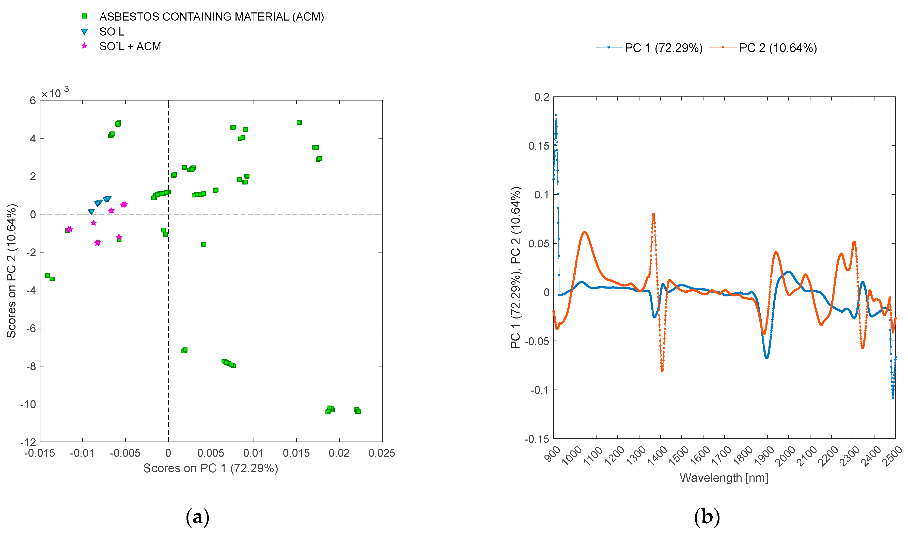
Soil, ACM and soil mixed with ACM (‘ACM’, ‘SOIL’, and ‘SOIL + ACM’ classes).
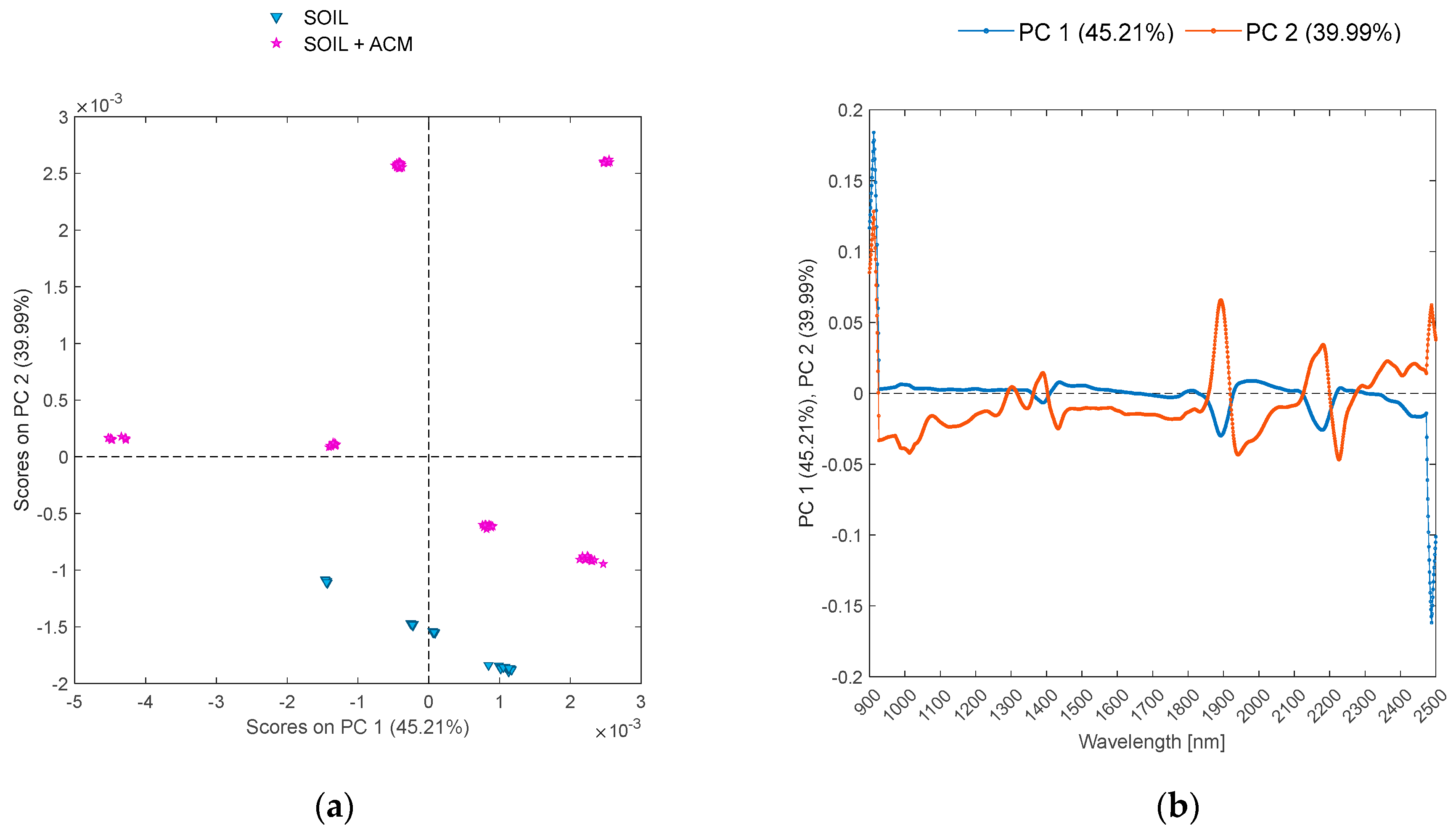
Soil and soil mixed with ACM (‘SOIL’ and ‘SOIL + ACM’ classes).
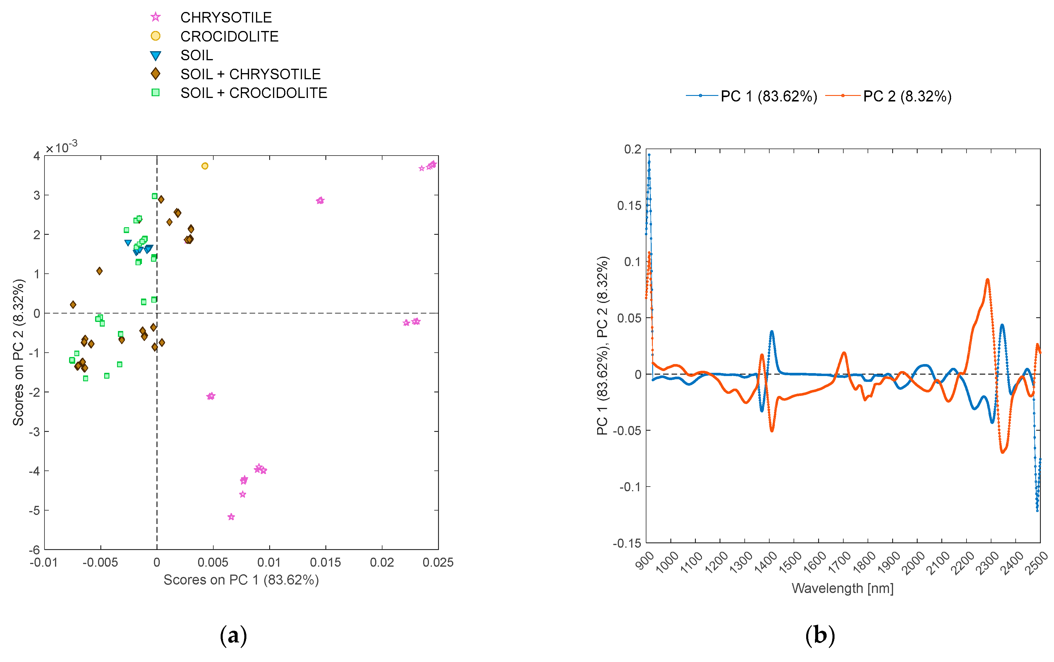
Soil, chrysotile, crocidolite, and soil–chrysotile/soil–crocidolite mixtures (‘SOIL’, ‘CHRYSOTILE’, ‘CROCIDOLITE’, ‘SOIL + CHRYSOTILE’, and ‘SOIL + CROCIDOLITE’ classes).
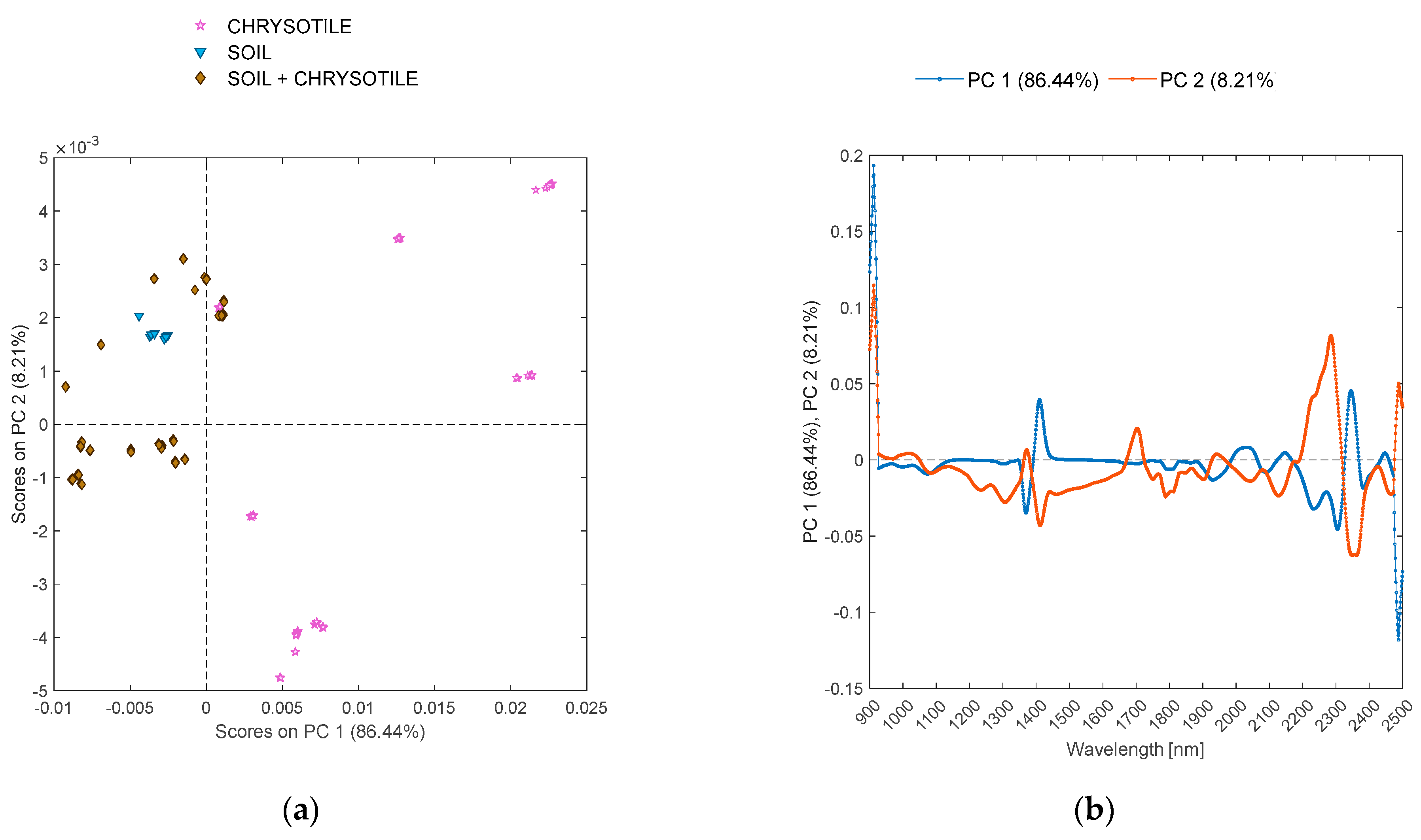
Soil, chrysotile, and soil–chrysotile mixtures (‘SOIL’, ‘CHRYSOTILE’, and ‘SOIL + CHRYSOTILE’ classes).
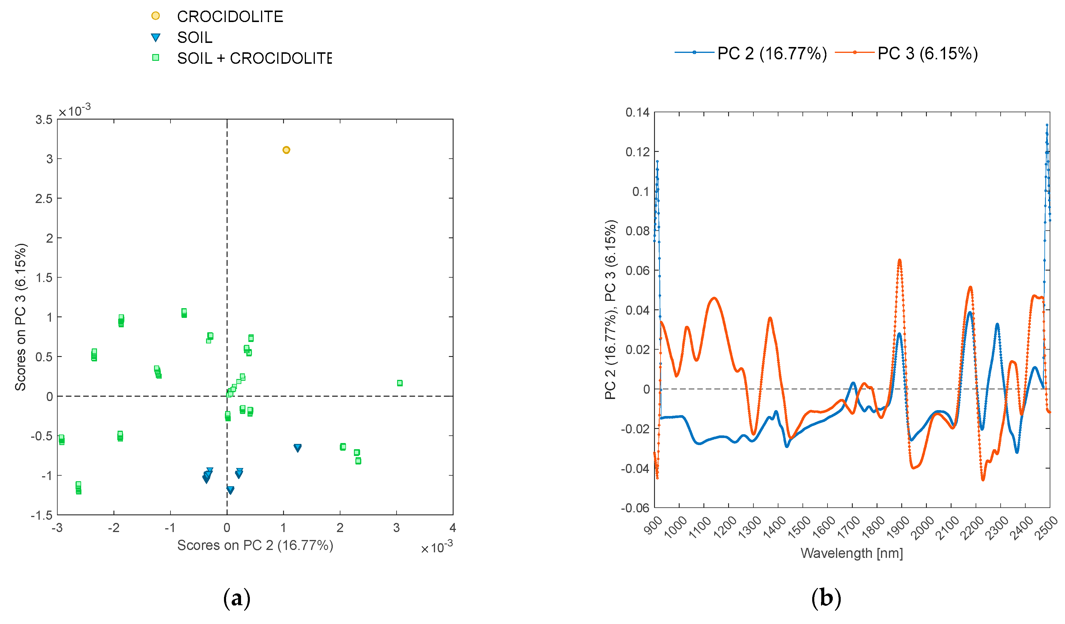
Soil, crocidolite, and soil–crocidolite mixtures (‘SOIL’, ‘CROCIDOLITE’, and ‘SOIL + CROCIDOLITE’ classes).
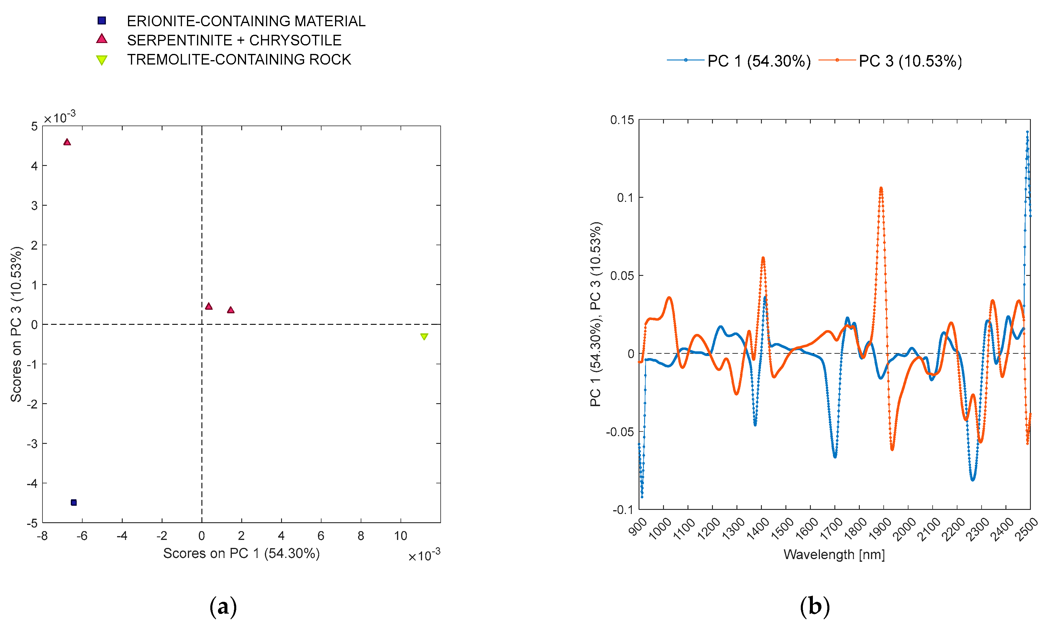
Naturally occurring asbestos and erionite-containing material samples (‘SERPENTINE+CHRYSOTILE’, ‘TREMOLITE-CONTAINING ROCK’, and ‘ERIONITE-CONTAINING MATERIAL’).

2.4. Classification Models and Performance Metrics

The main goal of a classification model is to identify the class a spectrum belongs to. In order to perform a classification, it is necessary to define a training set, where each spectrum is assigned to a class. During the classification, the classifier attempts to assign each analyzed element of the validation set to one of the previously defined classes. The setup of a classification model undergoes three main phases: (i) the calibration, during which the model is trained; (ii) the cross-validation, performed on the training set to define the PCs or latent variables (LVs) and designate the appropriate complexity of the model; and finally, (iii) the validation, during which the model is tested on a separate test set.

In order to build and validate the classification models, the DSO was randomly split into two parts by using the Kennard–Stone (K-S) algorithm, which is based on the Euclidean distance [44]. Seventy percent (70%) of the spectra were allocated to the training set, while the remaining thirty percent (30%) formed the test set. This split ensured class balance within the training and test sets; for example, 70% of the ‘CHRYSOTILE’ spectra were included in the training set, and the remaining 30% were placed in the test set. This division was achieved using a custom script written specifically for this purpose. The calibration and cross-validation of the model were performed on the training set, while the validation phase utilized the test set to evaluate the model’s predictive accuracy and robustness.

Different classification strategies commonly used in multivariate analyses, both linear and nonlinear, were tested to classify spectra according to the labels of the classes’ set ‘Category’ (refer to Table A1, Appendix A). The adopted classification strategies were partial least squares discriminant analysis (PLS-DA), principal component analysis-based discriminant analysis (PCA-DA), principal component analysis-based K-nearest neighbors classification (PCA-KNN), classification and regression trees (CART), and error-correcting output-coding support vector machine (ECOC-SVM) classifiers. The rationale for utilizing a diverse set of classification models in this study lies in the unique characteristics of spectral data and the need to optimize the classification performance. The utilization of linear (i.e., PLS-DA, PCA-DA) and nonlinear (i.e., CART, PCA-KNN and ECOC-SVM) techniques ensures the ability to capture different patterns and structures within the data. Each model offers distinct advantages and approaches to handling data variability, noise, and class separability. A detailed description of each classification technique is provided as follows.

2.4.1. Partial Least Squares Discriminant Analysis (PLS-DA)

The PLS-DA is one of the most used supervised techniques for pattern recognition in spectral classification. This method operates as an inverse least squares approach to linear discriminant analysis (LDA) and utilizes partial least squares (PLS) regression to predict the class label for each analyzed sample [45,46]. This model is particularly advantageous when dealing with correlated or collinear data, as it effectively extracts relevant information for class discrimination. In this study, the PLS-DA was set up on preprocessed reflectance spectra. The Venetian blinds (VB) method was used for cross-validation to determine the optimal number of LVs, ensuring the appropriate complexity of the model.

2.4.2. Principal Component Analysis-Based Discriminant Analysis (PCA-DA)

The LDA is a classification method that consists of calculating the so-called classification functions that are linear combinations of the original variables. These functions are designed to maximize the differences between groups, while minimizing differences within groups [47,48]. The classification functions are derived from a training set, where the class labels of samples are already known. The algorithm used in this study is a modification of Fisher’s discriminant functions. In this implementation, PCA was adopted as a dimensionality reduction tool prior to applying LDA [49]. The ideal number of PCs was evaluated using k-fold (k = 10) fold cross-validation. LDA was subsequently applied to the PCA-derived scores to perform the classification. PCA-DA is efficient for datasets with complex structures and overlapping features.

2.4.3. Principal Component Analysis-Based K-Nearest Neighbors Classification (PCA-KNN)

Among classification approaches, KNN is one of the simplest non-parametric algorithms widely used in various types of classification tasks [50,51]. This algorithm operates under the assumption that data points (spectra) exist within a feature (metric) space [52]. It identifies the k-nearest neighbors of a query vector (spectrum) based on a predefined distance metric, typically the Euclidean distance. It then assigns the class label of the query vector based on a majority vote among its nearest neighbors. The performance of a KNN classifier is highly dependent on the choice of k (the number of neighbors), as this parameter influences the classification results [53]. However, because KNN involves computing similarities across large datasets, its application is limited when handling high-dimensional spaces or very large training sets. To address this, KNN was performed on PCA scores, significantly reducing computation time and memory requirements without compromising classification efficiency. By reducing dimensions with PCA, this method mitigates the curse of dimensionality, while still capturing nonlinear relationships in the data. PCA-KNN is robust in handling small datasets and adaptable to complex class boundaries. Even in this case, the k-fold (k = 10) was used as the cross-validation method.

2.4.4. Classification and Regression Trees (CART)

Breiman et al. developed CART, a non-parametric statistical technique, in 1984 [54]. CART is one of the most widely used algorithms for solving both classification and regression problems [55,56]. In both types of problems, CART constructs a decision tree that describes a response variable as a function of various explanatory variables. The tree hierarchy consists of observation subsets as nodes, with the final nodes being the leaves. In CART, a binary division process is used at each node. During this process, spectra that meet the model’s criterion are grouped into one subgroup, while the rest are placed in another. The spectrum classification follows a path from the root to a final leaf, where the spectrum is assigned a class label. CART is particularly effective when the relationships between features and classes are complex and nonlinear.

In this case, the k-fold was used to select the optimal decision tree by evaluating the performance of the classifier.

2.4.5. Error-Correcting Output-Coding Support Vector Machine (ECOC SVM)

The ECOC SVM technique consists of an ECOC classifier that can be applied to multiclass problem, in which the classification method consists of various binary learners, such as support vector machines (SVMs) [57]. One of the key characteristics of SVMs is their reliance on structural risk minimization and their strong generalization capability [57]. By considering only the support vectors, which are a subset of the training points, SVMs determine the optimal separating hyperplane, leading to strong performance even with smaller training sets. SVMs are robust for handling high-dimensional data and are effective at finding optimal class boundaries in both linear and nonlinear spaces. There are two main strategies for addressing multiclass classification problems using SVM. The first approach involves creating multiple binary classifiers, while the second involves distinguishing all classes with a single classifier. In ECOC modelling, a multiclass (with three or more classes) classification problem is reduced to a set of binary classification tasks [58]. Given a multiclass classification task with

i

classes, the problem is decomposed as multiple binary classification problems, the so-called base classifiers [59]. This requires a coding design and a decoding scheme. The coding design specifies which classes the binary learners will train on, while the decoding scheme determines how the predictions from the base classifiers are aggregated. The output vector from each base classifier corresponds to the input vector of training samples, and this vector is then translated into a classification result using a code matrix in the decoding phase. ECOC is based on the error-correcting principles of communication theory. The core idea is to assign each class a unique error-correcting output codeword, ensuring optimal separation between the classes. ECOC-based modeling can enhance classification accuracy, offering an advantage over other multiclass classification models [60].

2.4.6. Metrics to Measure Classification Performance

The confusion matrix was considered to evaluate each classifier performance in calibration, cross-validation, and validation. The sensitivity, specificity, precision, accuracy, and misclassification error were calculated from the confusion matrices of each classifier for each considered class [46,61,62].

In a binary classification, sensitivity (Sens.), also known as recall, is the effectiveness of a classifier to identify positive labels (Equation (1)), while specificity (Spec.; Equation (2)) explains how effectively a classifier identifies negative labels. Precision (Prec.) represents the class agreement of the data labels with the positive labels given by the classifier (Equation (3)). While Accuracy (Acc.) is a metric of the overall effectiveness of a classifier (Equation (4)).

S e n s i t i v i t y (R e c a l l) = \frac{T P}{T P + F N}

(1)

S p e c i f i c i t y = \frac{T N}{F P + T N} = 1 - S e n s i t i v i t y

(2)

P r e c i s i o n = \frac{T P}{T P + F P}

(3)

A c c u r a c y = 1 - \frac{T P + F N}{T P + T N + F P + F N} = \frac{T P + T N}{T P + T N + F P + F N}

(4)

In Equations (1)–(4),

T P

(true positive) is a positive instance that is classified as positive,

F N

(false negative) is a positive instance that is classified as negative,

T N

(true negative) is a negative instance that is a classified as negative, and

F P (

false positive) is a negative instance that is classified as positive.

In a multiclass classification task, the input has to be classified into one and only one of

n

non-overlapping classes [63]. Measures for multiclass classification are based on a generalization of the Equations (1)–(4) for

n

C_{i}

classes.

{R e c a l l}_{M}

is the average per-class effectiveness of a classifier to identify class labels (Equation (5)), while

{A c c u r a c y}_{M}

represents the average per-class effectiveness of a classifier (Equation (6)). These two statistical parameters were considered to compare the overall performance of the classifiers.

{R e c a l l}_{M} = \frac{\sum_{i = 1}^{n} \frac{{T P}_{i}}{{T P}_{i} + {F N}_{i}}}{n}

(5)

A {c c u r a c y}_{M} = \frac{\sum_{i = 1}^{n} \frac{{T P}_{i} + {T N}_{i}}{{T P}_{i} + {T N}_{i} + {F P}_{i} + {F N}_{i}}}{n}

(6)

In order to compare the overall performances of the classifiers, statistical tests were performed where necessary. In more detail, to determine if the differences in model performance are statistically significant, a comparison of

{R e c a l l}_{M}

and

{A c c u r a c y}_{M}

metrics across calibration, cross-validation, and validation phases were performed using the Friedman test [64]. The Friedman test is a non-parametric statistical test used to detect differences in treatments across multiple test attempts. It is often used when the assumptions of the parametric repeated measures ANOVA (e.g., normality of data) are not met. While pairwise statistical comparisons between

{R e c a l l}_{M}

metrics of the classification models were conducted using the Student’s t-test. The Student’s t-test is a parametric test used to compare the means of two groups or conditions to determine whether they are significantly different from each other. The significance threshold was set at 0.05 for all the performed statistical tests.

3. Results and Discussion

3.1. Reflectance Spectra

In Figure 1, the raw reflectance and preprocessed spectra of the calibration set, averaged according to the ‘Category’ classes, are presented. As shown in Figure 1b, the combination of selected spectral preprocessing algorithms enhances peaks primarily in the first overtone of -OH stretching (1000–1500 nm), the H₂O bending (1600–1900 nm), and in the metal hydroxide combination bands (2100–2400 nm). These characteristic absorption peaks are typical of hydrated minerals and span broad ranges, with variations influenced by the chemical composition, particularly the metals present in their mineral structures [65,66,67]. In detail, strong reflectance changes are highlighted by the algorithms for the ‘CHRYSOTYLE’ class around 1300–1400 nm, 1800–1900 nm, and 2200–2400 nm, corresponding to -OH overtone and metal hydroxide vibrations commonly associated with serpentine minerals. In the preprocessed reflectance spectra, pronounced peaks of ‘CROCIDOLITE’ occur around 1100–1200 nm, 1300–1400 nm (-OH vibrations), and 1800–1900 nm (H₂O bending). The ‘AMOSITE’ class shows interesting features around 1000–1100 nm (-OH vibrations) and 1800–1900 nm (H₂O bending), with minor ones at 2200 and 2400 nm. Preprocessed reflectance ‘ERIONITE’ peaks appear to be mostly pronounced around 1400 nm (-OH stretching), 1800–1900 nm (H₂O bending), and 2300–2400 nm. Finally, the most pronounced peaks are found for ‘TREMOLITE’ at 1300–1500 nm (-OH overtone), 1600–1800 nm (H₂O bending), and 2100–2400 nm (metal hydroxide combinations). Most of the reported values correspond to data found in literature and spectral databases [65,66,67]. However, some discrepancies were noted; the peaks observed in the preprocessed spectra at 1100–1200 nm and 1800–1900 nm for ‘CROCIDOLITE’ and at 1800–1900 nm for ‘AMOSITE’ were not visible in the spectra of the same minerals in the USGS spectral library [67] (for additional details, refer to Appendix B). These discrepancies may result from sample preparation differences, matrix effects, or instrumental resolution.

Since hydrated minerals (e.g., silicates, carbonates) are the main constituents of both natural and anthropic matrices, absorptions features are also found in the same wavelength ranges for soils and ACMs.

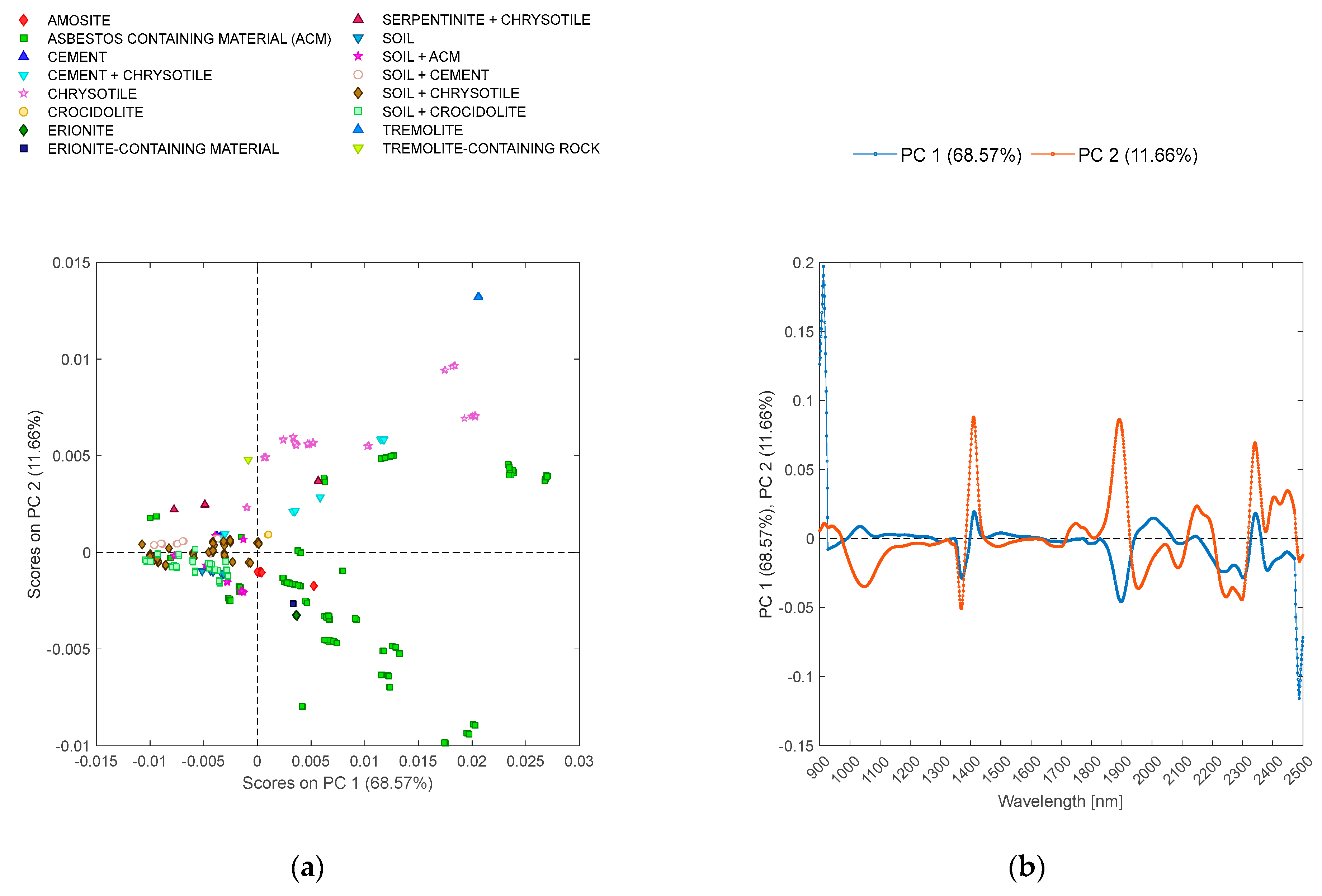
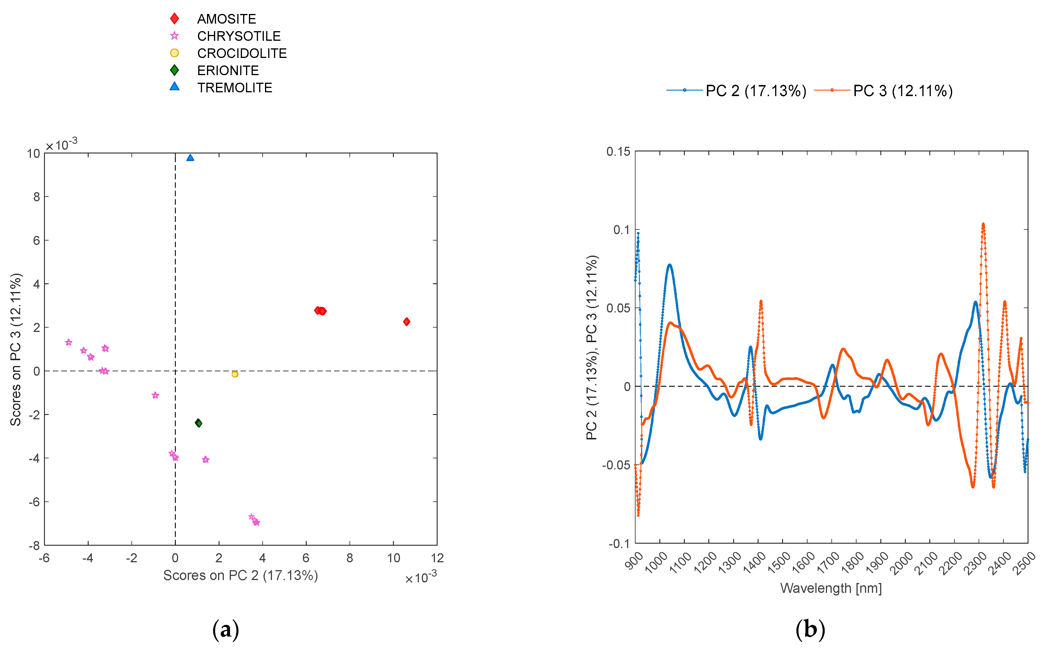
3.2. Principal Component Analysis

All samples. By applying the PCA to all spectra, a total variance of 98.2% was captured by using eight PCs. The relative scores were used to train the LDA and the KNN classifiers. The PCA scores and loading plots of the first two PCs for all the analyzed samples labelled according to ‘Category’ are reported in Figure 2. As shown in Figure 2a, a huge variability occurs in the considered dataset, and patterns underlying the scores are difficult to explore. However, some consideration about data can be made. PC1 captures 68.6% of variance, while PC2 the 11.7%. The scores of ‘ACM’ are mainly in the positive space of PC1, due to absorptions around 1000 and 2000 nm, while the ‘SOIL’ and soil-related classes scores are mostly in the negative space of PC1, due to absorptions at around 1380, 1900, 2200–2300, and 2350 nm. The ‘CEMENT’ scores are in the second quadrant, together with most of the NOA scores (‘SERPENTINITE+CRYSOTILE’ and ‘TREMOLITE-CONTAINING ROCK’), mainly due to absorptions at 1900 nm and 2350–2450 nm. The pure asbestos and erionite minerals scores, with the exception of tremolite, are in the positive space of PC1 due to the strong absorptions specifically around 1400 nm, 1900 nm, and 2300–2400 nm (Figure 2b).

Pure mineral samples. The PCA captures a total variance of 98.5% with six PCs by considering only the classes ‘CHRYSOTILE’, ‘CROCIDOLITE’, ‘AMOSITE’, ‘TREMOLITE’, and ‘ERIONITE’.

The PCA scores and loading plots of PC 2 and PC 3 for the analyzed samples of the considered classes are reported in Figure 3. PC 2 captures 17.1% of the variance, while PC 3 captures 12.1%.

The ‘CROCIDOLITE’, ‘AMOSITE’, ‘TREMOLITE’, and ‘ERIONITE’ scores are in the positive space of PC 2 (Figure 3a) due to the peaks in the loading scores at 1050 nm, 1370 nm, 1700 nm, 1900 nm, and 2250–2300 nm (Figure 3b). In more detail, ‘AMOSITE’ and ‘TREMOLITE’ are in the first quadrant due to the wavelength ranges mainly around 1000–1200 nm and 2300 nm. The ‘CROCIDOLITE’ and ‘ERIONITE’ scores are in the fourth quadrant due to the wavelength ranges around 1370 nm, 1700 nm, and 2280 nm.

The ‘CHRYSOTILE’ scores are in the second, third, and fourth quadrant, because this class includes six samples collected in different locations that probably do not have the same chemical composition. However, most of the scores are in the negative space of PC 2 due to the most pronounced peaks of the negative loading scores at 950 nm, 1410 nm, 1800 nm, 2130 nm, and 2350 nm.

Soil, ACM, and soil mixed with ACM. The PCA captures a total variance of 98.85% with seven PCs by considering only the three classes: ‘ACM’, ‘SOIL’, and ‘SOIL + ACM’. The PCA scores and loading plots of the first two principal components for the analyzed samples of the three classes are reported in Figure 4. The ACM scores are scattered in the four quadrants (Figure 4a). This is proof of the huge variability of the ACM samples considered, which includes different matrices but also different asbestos minerals. The scores related to soil and soil mixed with ACM in powder are instead placed in the negative space of PC1 due to the wavelengths around 1380 nm (first overtone of -OH stretching), 1850–1950 nm (first overtone of H₂O region), 2100–2300 nm (hydroxyl combination bands), and 2350 nm (combination bands of -OH stretching and Mg-OH deformation modes) [66].

Soil and soil mixed with ACM. The PCA captures a total variance of 98.5% with three principal components (PCs) by considering only the two classes: ‘SOIL’ and ‘SOIL + ACM’. The PCA scores and loading plots of the first two principal components for the analyzed samples of these two classes are presented in Figure 5. PC1 accounts for 45.2% of the variance, while PC2 explains 40% of the variance. The SOIL scores are in the negative space of PC2 (Figure 5a), mainly due to the wavelength ranges around 950–1050 nm, 1100–1200 nm, 1420–1450 nm, 1750 nm, 1900–2050 nm, and 2200–2250 nm, as indicated by the most pronounced peaks of the negative PC2 loadings in Figure 5b. The ‘SOIL + ACM’ scores are distributed across all quadrants except for quadrant III. These scores are highly clustered, with the number of groups (6 vs. 7) closely matching the number of samples.

Soil, chrysotile, crocidolite, and soil–chrysotile/soil–crocidolite mixtures. The PCA captures a total variance of 97.1% with three PCs by considering only the five classes ‘SOIL’, ‘CHRYSOTILE’, ‘CROCIDOLITE’, ‘SOIL + CHRYSOTILE’, and ‘SOIL + CROCIDOLITE’. The PCA scores and loading plots of the first two principal components for the analyzed samples of the considered five classes are reported in Figure 6.

The ‘CHRYSOTILE’ and ‘CROCIDOLITE’ scores are in the positive space of PC1 (Figure 6a) due to the wavelength ranges around 1400 nm and 2350 nm (Figure 6b), while the soil-related sample scores are in the negative space of PC1.

Soil, chrysotile, and soil–chrysotile mixtures. The PCA captures a total variance of 98.2% with three PCs by considering only the three classes ‘SOIL’, ‘CHRYSOTILE’, and ‘SOIL + CHRYSOTILE’.

The PCA scores and loading plots of PC 1 and PC 2 for the analyzed samples of the considered three classes are reported in Figure 7. As shown in the PCA score plot (Figure 7a), PC 1 captures 86.4% of the variance and separates ‘CHRYSOTILE’ from the other classes, due to the wavelength ranges around 1400 nm and 2350 nm (Figure 7b). However, the ‘SOIL + CHRYSOTILE’ and ‘SOIL’ scores are not easily separated by the explored PCs. The ‘SOIL’ scores are in the negative space of PC1 and positive space of PC2 due to the wavelengths around 1400 nm and 2200–2300 nm, which are typical of Al-rich clays, such as illite/muscovite (refer to [67]—Illite CU00-5B Hi-Al+Quartz ASDFRa AREF), as reported in Figure A2 (Appendix B).

Soil, crocidolite, and soil–crocidolite mixtures. The PCA captures a total variance of 97.8% with only three PCs by considering the three classes ‘SOIL’, ‘CROCIDOLITE’, and ‘SOIL + CROCIDOLITE’.

The PCA scores and loading plots of PC 2 and PC 3 for the analyzed samples of the considered three classes are reported in Figure 8.

PC 2 captures 16.8% of the variance, while PC 3 captures 6.2%. PC 2 separates ‘CROCIDOLITE’ from the soil–crocidolite mixture scores (Figure 8a), due to the wavelength ranges around 1800–1900 nm, 2100–2200 nm, and 2450 nm (Figure 8b). However, the ‘SOIL + CROCIDOLITE’ and ‘SOIL’ scores are not easily separated by the explored PCs. In more detail, all SOIL scores are in the negative space of PC3 due to the wavelengths around 1300 nm and 1400–1700 nm, 1900–2100 nm, 2200–2300 nm, and 2380 nm.

Naturally occurring asbestos and erionite-containing material. The PCA captures a total variance of 100% with four PCs by considering only the classes ‘SERPENTINE+CHRYSOTILE’, ‘TREMOLITE-CONTAINING ROCK’, and ‘ERIONITE-CONTAINING MATERIAL’.

The PCA scores and loading plots of PC 1 and PC 3 for the analyzed samples of the considered classes are reported in Figure 9. PC 1 captures 54.3% of the variance, while PC 3 captures 10.5%. The ‘SERPENTINE+CHRYSOTILE’ scores are in the positive space of PC 3 (Figure 9a), due to the wavelengths around 1000 nm, 1400 nm, 1900 nm, 2350 nm, and 2450 nm (Figure 9b). The ‘ERIONITE-CONTAINING MATERIAL’ scores are in the third quadrant of the score plot, due to the wavelengths around 2100 nm and 2200–2300 nm. Finally, the ‘TREMOLITE-CONTAINING ROCK’ scores are in the fourth quadrant, due to the wavelengths around 1200–1300 nm, 1450–1500 nm, and 2300 nm.

4. Classification Performances

4.1. PLS-DA

Eight LVs were used to perform the PLS-DA. The performance indices calculated from the confusion matrices of the PLS-DA are shown in Table 1. The results of the PLS-DA model in the calibration, cross-validation, and validation phases indicate generally high sensitivity and specificity across various classes, with some exceptions, such as low precision and accuracy in distinguishing certain classes, like cement and soil mixtures containing asbestos. Sensitivity and specificity remain consistently high for key classes, like amosite, crocidolite, and tremolite, indicating robust classification performance for these asbestos minerals.

4.2. PCA-DA

The performance indices calculated from the confusion matrices of the PCA-DA are shown in Table 2. The PCA-DA model shows varied performance across different classes in calibration, cross-validation, and validation phases. While sensitivity and specificity are generally high for classes like crocidolite, tremolite, and erionite, there are notable challenges in accurately classifying certain materials, particularly cement and soil mixtures containing asbestos. Precision and accuracy also vary, indicating the need for further optimization to enhance classification performance, especially for complex sample compositions. Additionally, the model demonstrates some inconsistency in performance across the different modelling phases.

4.3. PCA-KNN

KNN was performed on PCA scores (PCs = 8) with a number of neighbors (k) set to one. The performance indices calculated from the confusion matrices of the PCA-KNN are shown in Table 3.

The PCA-KNN model demonstrates excellent performance across all phases, showing high sensitivity, specificity, precision, and accuracy and minimal misclassification error. This indicates that the KNN algorithm, when applied on PCA scores, effectively distinguishes between different classes of materials in the dataset. The model accurately identifies asbestos-containing materials as well as other classes with very low error rates, suggesting its robustness and reliability in classification tasks. However, slight variations in performance metrics between the cross-validation and validation phases imply some degree of variability in generalization. In more detail, notable drops in sensitivity and precision are observed for a few specific classes, such as ‘CEMENT’ (sensitivity: 0.83, precision: 0.83) and ‘SOIL + CROCIDOLITE’ (sensitivity: 0.98, precision: 0.93). These discrepancies highlight some challenges in consistently classifying these categories in the validation phase. In this specific case, the model’s generalization capability could be further optimized, possibly through additional training data or parameter fine-tuning.

4.4. CART

The results obtained by the confusion matrices of the classification trees (binary decision trees for multiclass learning) with 53 nodes are shown in Table 4. The results from CART model demonstrate exceptional performance across all phases of the modeling process, including calibration, cross-validation, and validation. The model shows perfect sensitivity, specificity, precision, and accuracy for all classes, indicating its robustness and reliability in classifying different materials. This is also supported by the fact that the potential for overfitting was mitigated by employing cross-validation and pruning techniques to balance model complexity and generalizability.

4.5. ECOC SVM

The ECOC SVM model demonstrates outstanding performance across all phases of the modelling process, including calibration, cross-validation, and validation. The results, as shown in Table 5, exhibit perfect sensitivity, specificity, precision, and accuracy and no misclassification error for all classes, indicating the model’s robustness and reliability in classifying different materials. To generalize and mitigate the potential for overfitting, cross-validation was rigorously employed during the modeling process, supporting the model’s effectiveness. With consistent perfect scores in all metrics across the phases, the ECOC SVM model proves to be highly effective in accurately classifying materials in the dataset.

4.6. Classifiers Comparison

The comparison of classifier performance metrics, as reported in Table 6, reveals distinct trends across the different setup models. The Friedman tests performed to compare the metrics across the five classifiers during the calibration, cross-validation, and validation phases yielded significant results for both

{R e c a l l}_{M}

(χ²(4) = 12, p = 0.021) and

{A c c u r a c y}_{M}

(χ²(4) =12, p = 0.017).

Among the classifiers, ECOC SVM and CART consistently demonstrate the highest performance across all phases of modeling, with perfect macro-average recall and average accuracy scores of 1.00.

PCA-KNN performances were comparable to CART, even if slightly worse (recall: t(4) = −1.732, p = 0.158) and ECOC SVM (recall: t(4) = −1.732, p = 0.158) with

{R e c a l l}_{M}

values ranging from 0.98 to 1.00 and an

{A c c u r a c y}_{M}

equal to 1.00 across all phases. Although not perfect, PCA-KNN still exhibits high accuracy and recall rates, positioning it as a strong performer in comparison to other classifiers.

On the other hand, both PCA-DA and PLS-DA show comparatively poorer performances. In more detail, with PCA-DA are obtained a

{R e c a l l}_{M}

of 0.66–0.70 and an

{A c c u r a c y}_{M}

equal to 0.95, while for the PLS-DA a

{R e c a l l}_{M}

of 0.68–0.74 and an

{A c c u r a c y}_{M}

equal to 0.95 are achieved.

5. Conclusions and Future Perspectives

This study has shown the potential of portable instrumentation for the on-field assessment of asbestos presence in both natural and anthropogenic matrices. In more detail, the use of a spectrophotoradiometer operating in the visible and short-wave infrared range assisted by chemometrics and machine learning techniques allows for the discrimination of different samples of pure asbestos and asbestiform minerals (e.g., erionite), NOA, anthropic ACMs, clay–soil, Portland cement, and different mixtures of soil/pure asbestos, soil/ACM, cement/pure asbestos. Principal component analysis showed the high variability occurring among the collected data, underscoring the complexity of the analyzed matrices. Five different classification strategies commonly used in multivariate analyses, both linear and nonlinear, were tested to identify the different samples. The tested classifiers showed different performances in discriminating the analyzed samples. CART and ECOC SVM performed at best, followed by PCA-KNN. The performance of these classifiers was not influenced by the different grain size ranges of the considered samples. Instead, poorer performances were obtained by PLS-DA and PCA-DA.

Vis-SWIR hand-held spectrometers proved to be reliable, cost-effective tools for rapid and accurate on-field asbestos detection, enabling direct and noninvasive analysis. Their methodological precision, combined with the robustness of machine learning techniques, offers a significant advantage by minimizing the risk of airborne fiber exposure for technicians and reducing the need for destructive sampling. Compared to traditional methods, which often require complex sample preparation and laboratory infrastructure, this approach offers significant practical benefits for real-time asbestos detection and management.

Despite its benefits, the real-world deployment of this approach may face challenges, such as environmental factors (e.g., humidity, temperature, or sample heterogeneity), that could affect SWIR spectroscopy measurements accuracy. Future studies should systematically evaluate these factors to optimize the methodology for diverse field conditions. Additionally, integrating this technique into routine safety practices and regulatory frameworks can enhance its practical applicability. This may involve developing standardized protocols for on-field measurements and providing training to operators in diverse industrial and environmental contexts.

Future research should focus on building an extensive spectral library of both anthropogenic and natural materials to enhance the robustness and versatility of the method. This could involve specific experimental steps, such as collecting and analyzing field data from diverse geographic locations or industrial sites. Collaborations with regulatory agencies and industrial partners could also help ensure the library’s comprehensiveness and applicability across varied conditions. Such an approach would support the application of Vis-SWIR hand-held spectrometers in more complex scenarios, i.e., the characterization and management of excavated earth, post-earthquake building debris, and CDW. Moreover, incorporating real-time processing capabilities for large datasets could enhance the scalability and efficiency of this method, making it better suited for widespread industrial applications.

Such an application can contribute directly to the United Nations’ SDGs, particularly SDG 3 (Good Health and Well-Being), by advancing human health protection through improved asbestos detection, and SDG 12 (Responsible Consumption and Production), by promoting sustainable, low-waste analytical practices.

Author Contributions

G.B., R.G., G.C. and S.S. conceived the experiments. R.G., I.L., S.M. and G.C. conducted the experiments. G.B., R.G., G.C. and S.S. performed the spectral analyses. G.B., R.G., G.C., I.L., S.M. and S.S. analyzed the results. I.L., S.B., F.P. and S.M. discussed the results. All authors have read and agreed to the published version of the manuscript.

Funding

This research received no external funding.

Institutional Review Board Statement

Not applicable.

Informed Consent Statement

Not applicable.

Data Availability Statement

The datasets generated during and/or analyzed during the study are available from the corresponding author on reasonable request.

Acknowledgments

The study was developed in the framework of INAIL (Italian National Institute for Insurance against Accidents at Work) project ID71-2022: Sviluppo di strumentazione innovative mediante tecniche di rilevamento ed elaborazione ottica e spettrale on-site.

Conflicts of Interest

The authors declare that they have no known competing financial interests or personal relationships that could have appeared to influence the work reported in this paper.

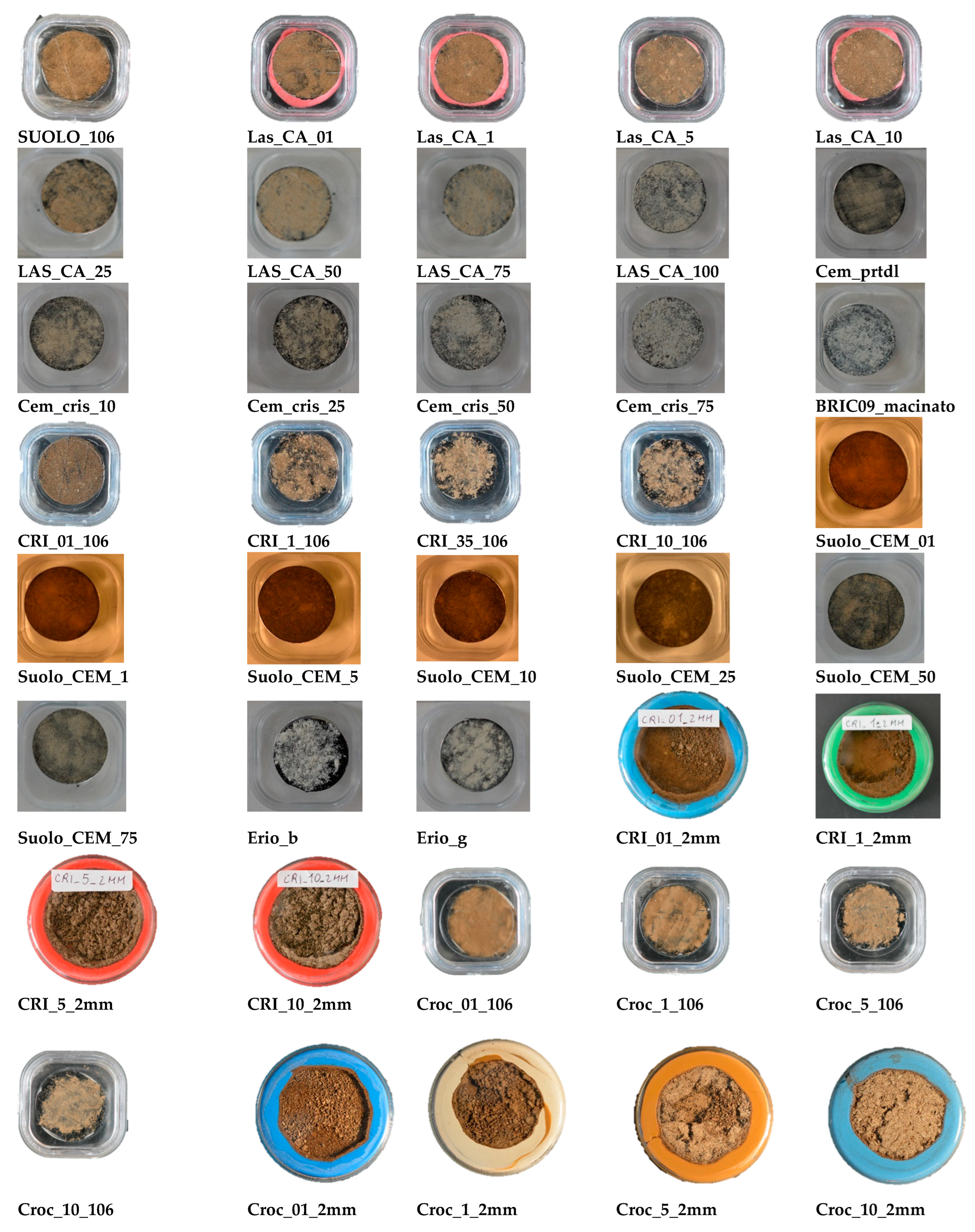
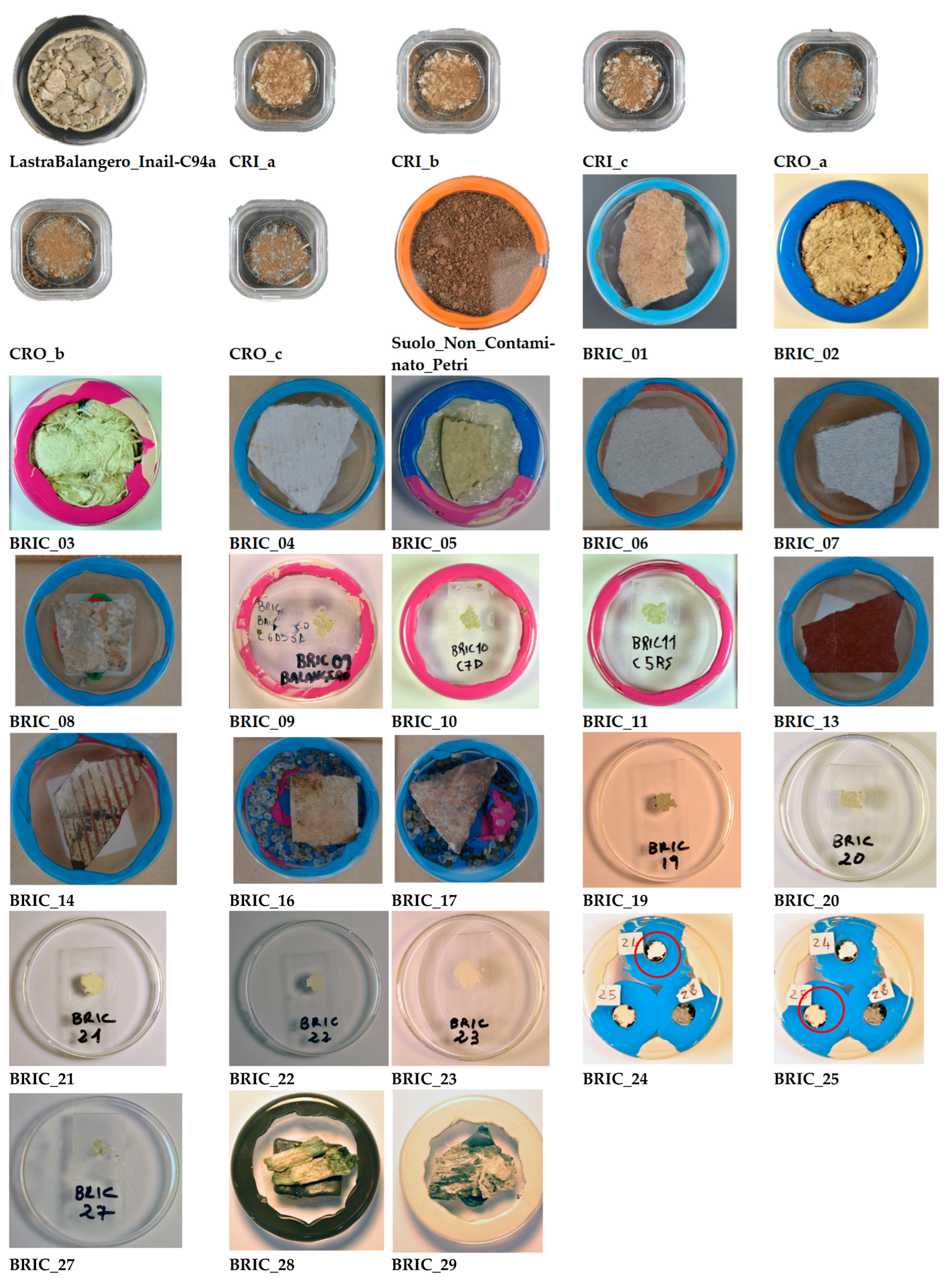
Appendix A. Analyzed Samples

In this appendix, the detail of the analyzed samples is reported as a complement to Section 2.1 ‘Analyzed samples’. In more detail, sample images are reported in Figure A1, while their description and classification are defined in Table A1.

Figure A1. Analyzed samples of pure asbestos, natural and anthropic ACMs, soil, cement, and mixtures.

Table A1. Description of the analyzed samples.

Sample’s ID	Sample Description	Casing	Category
Erio_b	Erionite at 98% (Bric 39)	SEM Specimen Stub (25 mm diameter)	ERIONITE
Erio_g	Erionite at 40% (Bric 40)	SEM Specimen Stub (25 mm diameter)	ERIONITE-CONTAINING MATERIAL
Cem_prtdl	Milled Portland Cement	SEM Specimen Stub (25 mm diameter)	CEMENT
LAS_100	Hand-ground asbestos–cement slab from Balangero’s industrial site (Piedmont, Italy)	SEM Specimen Stub (25 mm diameter)	ASBESTOS-CONTAINING MATERIAL (ACM)
BRIC09_macinato	Milled chrysotile from Balangero’s mining site	SEM Specimen Stub (25 mm diameter)	CHRYSOTILE
SUOLO_106	Monte Porzio Catone (MPC)’s (Roma, Italy) topsoil, hand-ground with granulometry < 106 μm	SEM Specimen Stub (25 mm diameter)	SOIL
Cem_cris_10	Portland cement + Balangero’s chrysotile (10 wt%)	SEM Specimen Stub (25mm diameter)	CEMENT + CHRYSOTILE
Cem_cris_25	Portland cement + Balangero’s chrysotile (25 wt%)	SEM Specimen Stub (25mm diameter)	CEMENT + CHRYSOTILE
Cem_cris_50	Portland cement + Balangero’s chrysotile (50 wt%)	SEM Specimen Stub (25mm diameter)	CEMENT + CHRYSOTILE
Cem_cris_75	Portland cement + Balangero’s chrysotile (75 wt%)	SEM Specimen Stub (25mm diameter)	CEMENT + CHRYSOTILE
Las CA 01	MPC’s soil < 106 μm + hand-ground asbestos–cement slab from Balangero’s mining site (0.1 wt%)	SEM Specimen Stub (25mm diameter)	SOIL + ACM
Las CA 1	MPC’s soil < 106 μm + hand-ground asbestos–cement slab from Balangero’s mining site (1 wt%)	SEM Specimen Stub (25mm diameter)	SOIL + ACM
Las CA 5	MPC’s soil <1 06 μm + hand-ground asbestos–cement slab from Balangero’s mining site (5 wt%)	SEM Specimen Stub (25mm diameter)	SOIL + ACM
Las CA 10	MPC’s soil < 106 μm + hand-ground asbestos–cement slab from Balangero’s mining site (10 wt%)	SEM Specimen Stub (25mm diameter)	SOIL + ACM
LAS_CA_25	MPC’s soil < 106 μm + hand-ground asbestos–cement slab from Balangero’s mining site (25 wt%)	SEM Specimen Stub (25mm diameter)	SOIL + ACM
LAS_CA_50	MPC’s soil < 106 μm + hand-ground asbestos–cement slab from Balangero’s mining site (50 wt%)	SEM Specimen Stub (25mm diameter)	SOIL + ACM
LAS_CA_75	MPC’s soil < 106 μm + hand-ground asbestos–cement slab from Balangero’s mining site (75 wt%)	SEM Specimen Stub (25mm diameter)	SOIL + ACM
Suolo_CEM_01	MPC’s soil < 106 μm + Portland cement (0.1 wt%)	SEM Specimen Stub (25mm diameter)	SOIL + CEMENT
Suolo_CEM_1	MPC’s soil < 106 μm + Portland cement (1 wt%)	SEM Specimen Stub (25mm diameter)	SOIL + CEMENT
Suolo_CEM_5	MPC’s soil < 106 μm + Portland cement (5 wt%)	SEM Specimen Stub (25mm diameter)	SOIL + CEMENT
Suolo_CEM_10	MPC’s soil < 106 μm + Portland cement (10 wt%)	SEM Specimen Stub (25mm diameter)	SOIL + CEMENT
Suolo_CEM_25	MPC’s soil < 106 μm + Portland cement (25 wt%)	SEM Specimen Stub (25mm diameter)	SOIL + CEMENT
Suolo_CEM_50	MPC’s soil < 106 μm + Portland cement (50 wt%)	SEM Specimen Stub (25mm diameter)	SOIL + CEMENT
Suolo_CEM_75	MPC’s soil < 106 μm + Portland cement (75 wt%)	SEM Specimen Stub (25mm diameter)	SOIL + CEMENT
CRI_01_106	MPC’s soil < 106 μm + Balangero’s chrysotile (0.1 wt%)	SEM Specimen Stub (25mm diameter)	SOIL + CHRYSOTILE
CRI_1_106	MPC’s soil < 106 μm + Balangero’s chrysotile (1 wt%)	SEM Specimen Stub (25mm diameter)	SOIL + CHRYSOTILE
CRI_35_106	MPC’s soil < 106 μm + Balangero’s chrysotile (3.5 wt%)	SEM Specimen Stub (25mm diameter)	SOIL + CHRYSOTILE
CRI_10_106	MPC’s soil < 106 μm + Balangero’s chrysotile (10 wt%)	SEM Specimen Stub (25mm diameter)	SOIL + CHRYSOTILE
CRI_01_2mm	MPC’s soil < 2 mm + Balangero chrysotile (0.1 wt%)	Borosilicate petri dish (60 mm diameter)	SOIL + CHRYSOTILE
CRI_1_2mm	MPCs’ soil < 2 mm + Balangero chrysotile (1 wt%)	Borosilicate petri dish (60 mm diameter)	SOIL + CHRYSOTILE
CRI_5_2mm	MPC’s soil < 2 mm + Balangero chrysotile (5 wt%)	Borosilicate petri dish (60 mm diameter)	SOIL + CHRYSOTILE
CRI_10_2mm	MPC’s soil < 2 mm + Balangero’s chrysotile (10 wt%)	Borosilicate petri dish (60 mm diameter)	SOIL + CHRYSOTILE
Croc_01_106	MPC’s soil < 106 μm + crocidolite (0.1 wt%)	SEM Specimen Stub (25mm diameter)	SOIL + CROCIDOLITE
Croc_1_106	MPC’s soil < 106 μm + crocidolite (1 wt%)	SEM Specimen Stub (25mm diameter)	SOIL + CROCIDOLITE
Croc_5_106	MPC’s soil < 106 μm + crocidolite (5 wt%)	SEM Specimen Stub (25mm diameter)	SOIL + CROCIDOLITE
Croc_10_106	MPC’s soil < 106 μm + crocidolite (10 wt%)	SEM Specimen Stub (25mm diameter)	SOIL + CROCIDOLITE
Croc_01_2mm	MPC’s soil < 2 mm + crocidolite (0.1 wt%)	Borosilicate petri dish (60 mm diameter)	SOIL + CROCIDOLITE
Croc_1_2mm	MPC’s soil < 2 mm + crocidolite (1 wt%)	Borosilicate petri dish (60 mm diameter)	SOIL + CROCIDOLITE
Croc_5_2mm	MPC’s soil < 2 mm + crocidolite (5 wt%)	Borosilicate petri dish (60 mm diameter)	SOIL + CROCIDOLITE
Croc_10_2mm	MPC’s soil < 2 mm + crocidolite (10 wt%)	Borosilicate petri dish (60 mm diameter)	SOIL + CROCIDOLITE
LastraBalangero_Inail-C94a	Hand-ground asbestos–cement slab from Balangero’s mining site	Borosilicate petri dish (60 mm diameter)	ASBESTOS-CONTAINING MATERIAL (ACM)
CRI_a	Chrysotile massively deposited all over the stub and MPC’s soil deposited in the empty spaces	SEM Specimen Stub (25mm diameter)	SOIL + CHRYSOTILE
CRI_b	Chrysotile massively deposited all over the stub and MPC’s soil deposited in the empty spaces	SEM Specimen Stub (25mm diameter)	SOIL + CHRYSOTILE
CRI_c	Chrysotile massively deposited all over the stub and MPC’s soil deposited in the empty spaces	SEM Specimen Stub (25mm diameter)	SOIL + CHRYSOTILE
CRO_a	Crocidolite massively deposited all over the stub and MPC’s soil deposited in the empty spaces	SEM Specimen Stub (25mm diameter)	SOIL + CROCIDOLITE
CRO_b	Crocidolite massively deposited all over the stub and MPC’s soil deposited in the empty spaces	SEM Specimen Stub (25mm diameter)	SOIL + CROCIDOLITE
CRO_c	Crocidolite massively deposited all over the stub and MPC’s soil deposited in the empty spaces	SEM Specimen Stub (25mm diameter)	SOIL + CROCIDOLITE
Suolo_Non_Contaminato_Petri	MPC’s soil, hand-ground with granulometry < 2 mm	Borosilicate petri dish (60 mm diameter)	SOIL
BRIC_01	Wet corrugated asbestos–cement sheet	Borosilicate petri dish (60 mm diameter)	ASBESTOS-CONTAINING MATERIAL (ACM)
BRIC_02	Insulating asbestos-containing felt	Borosilicate petri dish (60 mm diameter)	ASBESTOS-CONTAINING MATERIAL (ACM)
BRIC_03	Asbestos-containing cord (diameter~5cm)	Borosilicate petri dish (60 mm diameter)	ASBESTOS-CONTAINING MATERIAL (ACM)
BRIC_04	Flat asbestos–cement sheet (thickness~1.5cm)	Borosilicate petri dish (60 mm diameter)	ASBESTOS-CONTAINING MATERIAL (ACM)
BRIC_05	Asbestos-containing gasket	Borosilicate petri dish (60 mm diameter)	ASBESTOS-CONTAINING MATERIAL (ACM)
BRIC_06	Asbestos-containing panel (thickness~0.5cm)	Borosilicate petri dish (60 mm diameter)	ASBESTOS-CONTAINING MATERIAL (ACM)
BRIC_07	Asbestos-containing panel (thickness~0.8cm)	Borosilicate petri dish (60 mm diameter)	ASBESTOS-CONTAINING MATERIAL (ACM)
BRIC_08	Asbestos–cement piping (diameter~20cm, thickness~2cm)	Borosilicate petri dish (60 mm diameter)	ASBESTOS-CONTAINING MATERIAL (ACM)
BRIC_09	Balangero’s chrysotile	Borosilicate petri dish (60 mm diameter)	CHRYSOTILE
BRIC_10	Balangero’s chrysotile	Borosilicate petri dish (60 mm diameter)	CHRYSOTILE
BRIC_11	Balangero’s chrysotile	Borosilicate petri dish (60 mm diameter)	CHRYSOTILE
BRIC_13	Vinyl–asbestos tile	Borosilicate petri dish (60 mm diameter)	ASBESTOS-CONTAINING MATERIAL (ACM)
BRIC_14	Vinyl–asbestos tile	Borosilicate petri dish (60 mm diameter)	ASBESTOS-CONTAINING MATERIAL (ACM)
BRIC_16	Piping with amosite	Borosilicate petri dish (60 mm diameter)	ASBESTOS-CONTAINING MATERIAL (ACM)
BRIC_17	Asbestos–cement slab	Borosilicate petri dish (60 mm diameter)	ASBESTOS-CONTAINING MATERIAL (ACM)
BRIC_19	Crocidolite (standard 5174)	Concave microscope slide in borosilicate petri dish	CROCIDOLITE
BRIC_20	Amosite (standard 312M)	Concave microscope slide in borosilicate petri dish	AMOSITE
BRIC_21	Chrysotile (standard intermediate 031G)	Concave microscope slide in borosilicate petri dish	CHRYSOTILE
BRIC_22	Chrysotile (standard intermediate 127H)	Concave microscope slide in borosilicate petri dish	CHRYSOTILE
BRIC_23	Tremolite fibers (standard NIEHS)	Concave microscope slide in borosilicate petri dish	TREMOLITE
BRIC_24	Chrysotile (standard NIEHS plastibest 20)	SEM Specimen Stub (12.5 mm diameter) in borosilicate petri dish	CHRYSOTILE
BRIC_25	Amosite (standard NIEHS)	SEM Specimen Stub (12.5 mm diameter) in borosilicate petri dish	AMOSITE
BRIC_27	Cement + chrysotile	SEM Specimen Stub (12.5 mm diameter) in borosilicate petri dish	CEMENT + CHRYSOTILE
BRIC_28	Rock with fibrous tremolite (Castelluccio Superiore, Italy)	SEM Specimen Stub (12.5 mm diameter) in borosilicate petri dish	TREMOLITE-CONTAINING ROCK
BRIC_29	Serpentinite with chrysotile (Balangero, Italy)	SEM Specimen Stub (12.5 mm diameter) in borosilicate petri dish	SERPENTINITE + CHRYSOTILE

Appendix B. Comparison of Spectra Within USGS Spectral Library

In Figure A2, a comparison of illite and chrysotile reflectance spectra retrieved from the USGS spectral library is reported. Additional information about the USGS Spectral Library Version 7 Data can be found at the following link: https://www.sciencebase.gov/catalog/item/5807a2a2e4b0841e59e3a18d, (accessed on 15 December 2024).

Figure A2. Comparison of raw reflectance spectra within USGS spectral library: Illite + quartz (s07_ASD_Illite_CU00-5B_Hi-Al+Quartz_ASDFRa_AREF.txt), chrysotile (coarse fibers) (s07_ASD_Chrysotile_ML99-12A_Coar_Fib_ASDFRb_AREF.txt), and chrysotile (fine fibers) (s07_ASD_Chrysotile_ML99-12C_Fine_Fib_ASDFRb_AREF.txt).

References

IARC Working Group on the Evaluation of Carcinogenic Risks to Humans. Arsenic, metals, fibres, and dusts. In IARC Monographs on the Evaluation of Carcinogenic Risks to Humans; International Agency for Research on Cancer: Lyon, France, 2012; Volume 100, p. 11. [Google Scholar]
IARC Working Group on the Evaluation of Carcinogenic Risks to Humans. Overall evaluations of carcinogenicity: And updating of IARC monographs. In IARC Monographs on the Evaluation of Carcinogenic Risks to Humans; No. Supplement 7; International Agency for Research on Cancer: Lyon, France, 1987; Volume 1–42, 440p. [Google Scholar]
IARC Working Group on the Evaluation of Carcinogenic Risks to Humans. Some Nanomaterials and Some Fibres. In IARC Monographs on the Evaluation of Carcinogenic Risks to Humans; International Agency for Research on Cancer: Lyon, France, 2017. [Google Scholar]
Lee, R.J.; Strohmeier, B.R.; Bunker, K.; Van Orden, D. Naturally occurring asbestos—A recurring public policy challenge. J. Hazard. Mater. 2008, 153, 1–21. [Google Scholar] [CrossRef]
National Minerals Information Center. Mineral Commodity Summaries 2022; USGS: Reston, VA, USA, 2022; p. 202. [Google Scholar]
Agency for Toxic Substances and Disease Registry. Toxicological Profile for Asbestos; Technical Report 1332-21-4; Department of Health and Human Services, Public Health Service: Atlanta, GA, USA, 2001. [Google Scholar]
Bowes, D.; Langer, A.; Rohl, A. Nature and range of mineral dusts in the environment. Philos. Trans. R. Soc. London. Ser. A Math. Phys. Sci. 1977, 286, 593–610. [Google Scholar]
Ricchiuti, C.; Bloise, A.; Punturo, R. Occurrence of asbestos in soils: State of the art. Epis. J. Int. Geosci. 2020, 43, 881–891. [Google Scholar] [CrossRef]
HSE. Asbestos: The Analysts’ Guide for Sampling, Analysis and Clearance Procedures (HSG 248); TSO: London, UK, 2006. [Google Scholar]
Malinconico, S.; Paglietti, F.; Serranti, S.; Bonifazi, G.; Lonigro, I. Asbestos in soil and water: A review of analytical techniques and methods. J. Hazard. Mater. 2022, 436, 129083. [Google Scholar] [CrossRef] [PubMed]
Stark, E.; Luchter, K. NIR instrumentation technology. NIR News 2005, 16, 13–16. [Google Scholar] [CrossRef]
Cen, H.; He, Y. Theory and application of near infrared reflectance spectroscopy in determination of food quality. Trends Food Sci. Technol. 2007, 18, 72–83. [Google Scholar] [CrossRef]
Davies, A.; Grant, A. Near infra-red analysis of food. Int. J. Food Sci. Technol. 1987, 22, 191–207. [Google Scholar] [CrossRef]
Cortés, V.; Blasco, J.; Aleixos, N.; Cubero, S.; Talens, P. Monitoring strategies for quality control of agricultural products using visible and near-infrared spectroscopy: A review. Trends Food Sci. Technol. 2019, 85, 138–148. [Google Scholar] [CrossRef]
Ozaki, Y. Near-infrared spectroscopy—Its versatility in analytical chemistry. Anal. Sci. 2012, 28, 545–563. [Google Scholar] [CrossRef]
Tekin, Y.; Kuang, B.; Mouazen, A.M. Potential of on-line visible and near infrared spectroscopy for measurement of pH for deriving variable rate lime recommendations. Sensors 2013, 13, 10177–10190. [Google Scholar] [CrossRef] [PubMed]
Luypaert, J.; Massart, D.; Vander Heyden, Y. Near-infrared spectroscopy applications in pharmaceutical analysis. Talanta 2007, 72, 865–883. [Google Scholar] [CrossRef] [PubMed]
Macho, S.; Larrechi, M.S. Near-infrared spectroscopy and multivariate calibration for the quantitative determination of certain properties in the petrochemical industry. TrAC Trends Anal. Chem. 2002, 21, 799–806. [Google Scholar] [CrossRef]
Heise, H.M. Medical applications of NIR spectroscopy. In Near-Infrared Spectroscopy; Springer: Berlin/Heidelberg, Germany, 2021; pp. 437–473. [Google Scholar]
Currà, A.; Gasbarrone, R.; Cardillo, A.; Fattapposta, F.; Missori, P.; Marinelli, L.; Bonifazi, G.; Serranti, S.; Trompetto, C. In vivo non-invasive near-infrared spectroscopy distinguishes normal, post-stroke, and botulinum toxin treated human muscles. Sci. Rep. 2021, 11, 17631. [Google Scholar] [CrossRef] [PubMed]
Bonifazi, G.; Capobianco, G.; Palmieri, R.; Serranti, S. Hyperspectral imaging applied to the waste recycling sector. Spectrosc. Eur. 2019, 31, 8–11. [Google Scholar] [CrossRef]
Bonifazi, G.; Fiore, L.; Gasbarrone, R.; Hennebert, P.; Serranti, S. Detection of Brominated Plastics from E-Waste by Short-Wave Infrared Spectroscopy. Recycling 2021, 6, 54. [Google Scholar] [CrossRef]
Turner, D.J.; Rivard, B.; Groat, L.A. Visible and short-wave infrared reflectance spectroscopy of REE phosphate minerals. Am. Mineral. 2016, 101, 2264–2278. [Google Scholar] [CrossRef]
Turner, D.J.; Rivard, B.; Groat, L.A. Visible and short-wave infrared reflectance spectroscopy of selected REE-bearing silicate minerals. Am. Mineral. J. Earth Planet. Mater. 2018, 103, 927–943. [Google Scholar] [CrossRef]
Catelli, E.; Sciutto, G.; Prati, S.; Chavez Lozano, M.V.; Gatti, L.; Lugli, F.; Silvestrini, S.; Benazzi, S.; Genorini, E.; Mazzeo, R. A new miniaturised short-wave infrared (SWIR) spectrometer for on-site cultural heritage investigations. Talanta 2020, 218, 121112. [Google Scholar] [CrossRef]
Rossel, R.V.; Cattle, S.R.; Ortega, A.; Fouad, Y. In situ measurements of soil colour, mineral composition and clay content by vis–NIR spectroscopy. Geoderma 2009, 150, 253–266. [Google Scholar] [CrossRef]
Shi, T.; Chen, Y.; Liu, Y.; Wu, G. Visible and near-infrared reflectance spectroscopy—An alternative for monitoring soil contamination by heavy metals. J. Hazard. Mater. 2014, 265, 166–176. [Google Scholar] [CrossRef] [PubMed]
Askari, M.S.; Cui, J.; O’Rourke, S.M.; Holden, N.M. Evaluation of soil structural quality using VIS–NIR spectra. Soil Tillage Res. 2015, 146, 108–117. [Google Scholar] [CrossRef]
Corradini, F.; Bartholomeus, H.; Lwanga, E.H.; Gertsen, H.; Geissen, V. Predicting soil microplastic concentration using vis-NIR spectroscopy. Sci. Total Environ. 2019, 650, 922–932. [Google Scholar] [CrossRef] [PubMed]
Wan, M.; Qu, M.; Hu, W.; Li, W.; Zhang, C.; Cheng, H.; Huang, B. Estimation of soil pH using PXRF spectrometry and Vis-NIR spectroscopy for rapid environmental risk assessment of soil heavy metals. Process Saf. Environ. Prot. 2019, 132, 73–81. [Google Scholar] [CrossRef]
Bonifazi, G.; Capobianco, G.; Serranti, S. Hyperspectral imaging applied to the identification and classification of asbestos fibers. In Proceedings of the 2015 IEEE SENSORS, Busan, Republic of Korea, 1–4 November 2015; pp. 1–4. [Google Scholar]
Zholobenko, V.; Rutten, F.; Zholobenko, A.; Holmes, A. In situ spectroscopic identification of the six types of asbestos. J. Hazard. Mater. 2021, 403, 123951. [Google Scholar] [CrossRef] [PubMed]
Bonifazi, G.; Capobianco, G.; Serranti, S. Asbestos containing materials detection and classification by the use of hyperspectral imaging. J. Hazard. Mater. 2018, 344, 981–993. [Google Scholar] [CrossRef]
Bonifazi, G.; Capobianco, G.; Serranti, S. Hyperspectral imaging and hierarchical PLS-DA applied to asbestos recognition in construction and demolition waste. Appl. Sci. 2019, 9, 4587. [Google Scholar] [CrossRef]
EN 197-1; Cement: Composition, Specifications and Conformity Criteria, Part 1: Common Cements. European Committee for Standardization: Brussels, Belgium, 2011.
ASD Inc. FieldSpec^® 4 User Manual, ASD Document 600979; ASD Inc.: Boulder, CO, USA, 2015. [Google Scholar]
ASD Inc. RS3™ User Manual, ASD Document 600545; ASD Inc.: Boulder, CO, USA, 2008.
Rinnan, Å.; Van Den Berg, F.; Engelsen, S.B. Review of the most common pre-processing techniques for near-infrared spectra. TrAC Trends Anal. Chem. 2009, 28, 1201–1222. [Google Scholar] [CrossRef]
Danner, M.; Locherer, M.; Hank, T.; Richter, K. Spectral Sampling with the ASD FIELDSPEC 4; GFZ Data Services: Potsdam, Germany, 2015. [Google Scholar]
Wise, B.M.; Gallagher, N.; Bro, R.; Shaver, J.; Windig, W.; Koch, R.S. PLS Toolbox 4.0; Eigenvector Research Inc.: Manson, WA, USA, 2007. [Google Scholar]
Van den Berg, R.A.; Hoefsloot, H.C.; Westerhuis, J.A.; Smilde, A.K.; Van der Werf, M.J. Centering, scaling, and transformations: Improving the biological information content of metabolomics data. BMC Genom. 2006, 7, 1–15. [Google Scholar] [CrossRef]
Wold, S.; Esbensen, K.; Geladi, P. Principal component analysis. Chemom. Intell. Lab. Syst. 1987, 2, 37–52. [Google Scholar] [CrossRef]
Bro, R.; Smilde, A.K. Principal component analysis. Anal. Methods 2014, 6, 2812–2831. [Google Scholar] [CrossRef]
Kennard, R.W.; Stone, L.A. Computer aided design of experiments. Technometrics 1969, 11, 137–148. [Google Scholar] [CrossRef]
Barker, M.; Rayens, W. Partial least squares for discrimination. J. Chemom. A J. Chemom. Soc. 2003, 17, 166–173. [Google Scholar] [CrossRef]
Ballabio, D.; Consonni, V. Classification tools in chemistry. Part 1: Linear models. PLS-DA. Anal. Methods 2013, 5, 3790–3798. [Google Scholar] [CrossRef]
Fisher, R.A. The use of multiple measurements in taxonomic problems. Ann. Eugen. 1936, 7, 179–188. [Google Scholar] [CrossRef]
Bruns, R.; Faigle, J. Quimiometria. Química Nova 1985, 8, 84–99. [Google Scholar]
Kemsley, E.K. Discriminant analysis of high-dimensional data: A comparison of principal components analysis and partial least squares data reduction methods. Chemom. Intell. Lab. Syst. 1996, 33, 47–61. [Google Scholar] [CrossRef]
Parvin, H.; Alizadeh, H.; Minaei-Bidgoli, B. MKNN: Modified k-nearest neighbor. In Proceedings of the World Congress on Engineering and Computer Science, San Francisco, CA, USA, 22–24 October 2008. [Google Scholar]
Guo, G.; Wang, H.; Bell, D.; Bi, Y.; Greer, K. KNN model-based approach in classification. In Proceedings of the OTM Confederated International Conferences “On the Move to Meaningful Internet Systems”, Catania, Sicily, Italy, 3–7 November 2003; pp. 986–996. [Google Scholar]
Chitari, A.; Bag, V. Detection of brain tumor using classification algorithm. Int. J. Invent. Comput. Sci. Eng 2014, 1, 2348–3539. [Google Scholar]
Imandoust, S.B.; Bolandraftar, M. Application of k-nearest neighbor (knn) approach for predicting economic events: Theoretical background. Int. J. Eng. Res. Appl. 2013, 3, 605–610. [Google Scholar]
Breiman, L.; Friedman, J.H.; Olshen, R.A.; Stone, C.J. Classification and Regression Trees; Routledge: London, UK, 2017. [Google Scholar]
Lewis, R.J. An introduction to classification and regression tree (CART) analysis. In Proceedings of the Annual Meeting of the Society for Academic Emergency Medicine, San Francisco, CA, USA, 22–25 May 2000. [Google Scholar]
Timofeev, R. Classification and Regression Trees (CART) Theory and Applications; Humboldt University: Berlin, Germany, 2004; Volume 54. [Google Scholar]
Xiao-Feng, L.; Xue-ying, Z.; Ji-Kang, D. Speech recognition based on support vector machine and error correcting output codes. In Proceedings of the 2010 First International Conference on Pervasive Computing, Signal Processing and Applications, Harbin, China, 17–19 September 2010; pp. 336–339. [Google Scholar]
Hatami, N. Thinned-ECOC ensemble based on sequential code shrinking. Expert Syst. Appl. 2012, 39, 936–947. [Google Scholar] [CrossRef]
He, X.; Wang, Z.; Jin, C.; Zheng, Y.; Xue, X. A simplified multi-class support vector machine with reduced dual optimization. Pattern Recognit. Lett. 2012, 33, 71–82. [Google Scholar] [CrossRef]
Zhou, Y.; Fang, K.; Yang, M.; Ma, P. An Intelligent Model Validation Method Based on ECOC SVM. In Proceedings of the 10th International Conference on Computer Modeling and Simulation, Sydney, Australia, 8–10 January 2018; pp. 67–71. [Google Scholar]
Ballabio, D.; Grisoni, F.; Todeschini, R. Multivariate comparison of classification performance measures. Chemom. Intell. Lab. Syst. 2018, 174, 33–44. [Google Scholar] [CrossRef]
Fawcett, T. An introduction to ROC analysis. Pattern Recognit. Lett. 2006, 27, 861–874. [Google Scholar] [CrossRef]
Grandini, M.; Bagli, E.; Visani, G. Metrics for multi-class classification: An overview. arXiv 2020, arXiv:2008.05756. [Google Scholar]
Rainio, O.; Teuho, J.; Klén, R. Evaluation metrics and statistical tests for machine learning. Sci. Rep. 2024, 14, 6086. [Google Scholar] [CrossRef] [PubMed]
Lewis, I.R.; Chaffin, N.C.; Gunter, M.E.; Griffiths, P.R. Vibrational spectroscopic studies of asbestos and comparison of suitability for remote analysis. Spectrochim. Acta—Part A Mol. Spectrosc. 1996, 52, 315–328. [Google Scholar] [CrossRef]
Clark, R.N.; King, T.V.V.; Klejwa, M.; Swayze, G.A.; Vergo, N. High spectral resolution reflectance spectroscopy of minerals. J. Geophys. Res. Solid Earth 1990, 95, 12653–12680. [Google Scholar] [CrossRef]
USGS Spectral Library Version 7. 2017. Available online: https://pubs.usgs.gov/publication/ds1035 (accessed on 15 December 2024).

Figure 1. Raw reflectance (a) and preprocessed (b) spectra (900–2500 nm) of all the analyzed samples averaged according to the material class set (‘Category’).

Figure 2. PCA score plot (a) and loading plot (b) of the first two principal components for all the analyzed samples labelled according to ‘Category’.

Figure 3. PCA score plot (a) and loading plot (b) of PC2 and PC3 for the analyzed samples of the classes ‘ERIONITE’, ‘CHRYSOTILE’, ‘AMOSITE’,’ CROCIDOLITE’, and ‘TREMOLITE’.

Figure 4. PCA score plot (a) and loading plot (b) of the first two principal components for the analyzed samples of the three classes ‘ACM’, ‘SOIL’, and ‘SOIL + ACM’.

Figure 5. PCA score plot (a) and loading plot (b) of the first two principal components for the analyzed samples of the two classes ‘SOIL’ and ‘SOIL + ACM’.

Figure 6. PCA score plot (a) and loading plot (b) of the first two principal components for the analyzed samples of the five classes ‘SOIL’, ‘CHRYSOTILE’, ‘CROCIDOLITE’, ‘SOIL + CHRYSOTILE’, and ‘SOIL + CROCIDOLITE’.

Figure 7. PCA score plot (a) and loading plot (b) of PC1 and PC2 for the analyzed samples of the three classes ‘SOIL’, ‘CHRYSOTILE’, and ‘SOIL + CHRYSOTILE’.

Figure 8. PCA score plot (a) and loading plot (b) of PC2 and PC3 for the analyzed samples of the three classes ‘SOIL’, ‘CROCIDOLITE’, and ‘SOIL + CROCIDOLITE’.

Figure 9. PCA score plot (a) and loading plot (b) of PC1 and PC3 for the analyzed samples of the classes ‘SERPENTINE + CHRYSOTILE’, ‘TREMOLITE-CONTAINING ROCK’, and ‘ERIONITE-CONTAINING MATERIAL’.

Table 1. Performance metrics of PLS-DA model in calibration (C), cross-validation (CV), and validation (V): sensitivity (Sens.), specificity (Spec.), precision (Prec.), accuracy (Acc.), and misclassification error (Err.).

Model Phase	Modelled Class	Sens.	Spec.	Err.	Prec.	Acc.
C	AMOSITE	1.00	0.99	0.01	0.56	0.99
	ASBESTOS-CONTAINING MATERIAL (ACM)	0.71	1.00	0.08	1.00	0.92
	CEMENT	0.00	1.00	0.01	-	0.99
	CEMENT + CHRYSOTILE	0.41	0.99	0.03	0.67	0.97
	CHRYSOTILE	0.90	0.99	0.02	0.93	0.98
	CROCIDOLITE	1.00	1.00	0.00	1.00	1.00
	ERIONITE	1.00	1.00	0.00	1.00	1.00
	ERIONITE-CONTAINING MATERIAL	1.00	1.00	0.00	1.00	1.00
	SERPENTINITE + CHRYSOTILE	1.00	1.00	0.00	1.00	1.00
	SOIL	0.82	0.96	0.04	0.42	0.96
	SOIL + ACM	0.27	0.86	0.18	0.11	0.82
	SOIL + CEMENT	0.89	0.93	0.07	0.44	0.93
	SOIL + CHRYSOTILE	0.20	0.96	0.17	0.48	0.83
	SOIL + CROCIDOLITE	0.60	0.90	0.15	0.54	0.85
	TREMOLITE	1.00	1.00	0.00	1.00	1.00
	TREMOLITE-CONTAINING ROCK	1.00	1.00	0.00	1.00	1.00
CV	AMOSITE	1.00	0.99	0.01	0.56	0.99
	ASBESTOS-CONTAINING MATERIAL (ACM)	0.71	1.00	0.08	1.00	0.92
	CEMENT	0.00	1.00	0.01	-	0.99
	CEMENT + CHRYSOTILE	0.41	0.99	0.04	0.58	0.96
	CHRYSOTILE	0.90	0.99	0.02	0.93	0.98
	CROCIDOLITE	1.00	1.00	0.00	1.00	1.00
	ERIONITE	0.57	1.00	0.01	0.57	0.99
	ERIONITE-CONTAINING MATERIAL	0.57	1.00	0.01	0.57	0.99
	SERPENTINITE + CHRYSOTILE	1.00	1.00	0.00	1.00	1.00
	SOIL	0.82	0.96	0.05	0.40	0.95
	SOIL + ACM	0.23	0.86	0.18	0.10	0.82
	SOIL + CEMENT	0.89	0.93	0.07	0.45	0.93
	SOIL + CHRYSOTILE	0.19	0.96	0.17	0.48	0.83
	SOIL + CROCIDOLITE	0.60	0.90	0.15	0.54	0.85
	TREMOLITE	1.00	1.00	0.00	1.00	1.00
	TREMOLITE-CONTAINING ROCK	1.00	1.00	0.00	1.00	1.00
V	AMOSITE	1.00	0.97	0.03	0.40	0.97
	ASBESTOS-CONTAINING MATERIAL (ACM)	0.69	1.00	0.09	1.00	0.91
	CEMENT	0.00	1.00	0.01	-	0.99
	CEMENT + CHRYSOTILE	0.37	0.99	0.04	0.65	0.96
	CHRYSOTILE	0.94	0.99	0.02	0.87	0.98
	CROCIDOLITE	1.00	1.00	0.00	1.00	1.00
	ERIONITE	1.00	1.00	0.00	1.00	1.00
	ERIONITE-CONTAINING MATERIAL	1.00	1.00	0.00	1.00	1.00
	SERPENTINITE + CHRYSOTILE	1.00	1.00	0.00	1.00	1.00
	SOIL	0.58	0.97	0.04	0.41	0.96
	SOIL + ACM	0.26	0.87	0.17	0.11	0.83
	SOIL + CEMENT	0.79	0.93	0.08	0.42	0.92
	SOIL + CHRYSOTILE	0.20	0.97	0.16	0.55	0.84
	SOIL + CROCIDOLITE	0.70	0.89	0.14	0.55	0.86
	TREMOLITE	1.00	1.00	0.00	1.00	1.00
	TREMOLITE-CONTAINING ROCK	1.00	1.00	0.00	1.00	1.00

Table 2. Performance metrics of PCA-DA model in calibration (C), cross-validation (CV), and validation (V): sensitivity (Sens.), specificity (Spec.), precision (Prec.), accuracy (Acc.), and misclassification error (Err.).

Model Phase	Modelled Class	Sens.	Spec.	Err.	Prec.	Acc.
C	AMOSITE	1.00	0.99	0.01	0.56	0.99
	ASBESTOS-CONTAINING MATERIAL (ACM)	0.68	1.00	0.09	1.00	0.91
	CEMENT	0.29	1.00	0.01	0.57	0.99
	CEMENT + CHRYSOTILE	0.41	0.98	0.04	0.49	0.96
	CHRYSOTILE	0.80	0.99	0.03	0.92	0.97
	CROCIDOLITE	1.00	1.00	0.00	1.00	1.00
	ERIONITE	1.00	0.99	0.01	0.48	0.99
	ERIONITE-CONTAINING MATERIAL	1.00	1.00	0.00	1.00	1.00
	SERPENTINITE + CHRYSOTILE	0.29	0.99	0.03	0.46	0.97
	SOIL	0.00	1.00	0.03	-	0.97
	SOIL + ACM	0.00	0.94	0.12	0.00	0.88
	SOIL + CEMENT	0.89	0.94	0.07	0.47	0.93
	SOIL + CHRYSOTILE	0.73	0.87	0.16	0.52	0.84
	SOIL + CROCIDOLITE	0.52	0.89	0.17	0.46	0.83
	TREMOLITE	1.00	1.00	0.00	1.00	1.00
	TREMOLITE-CONTAINING ROCK	1.00	1.00	0.00	1.00	1.00
CV	AMOSITE	1.00	0.99	0.01	0.56	0.99
	ASBESTOS-CONTAINING MATERIAL (ACM)	0.69	1.00	0.09	1.00	0.91
	CEMENT	0.29	1.00	0.01	0.44	0.99
	CEMENT + CHRYSOTILE	0.40	0.98	0.05	0.45	0.95
	CHRYSOTILE	0.77	0.99	0.03	0.91	0.97
	CROCIDOLITE	1.00	1.00	0.00	1.00	1.00
	ERIONITE	1.00	0.99	0.01	0.56	0.99
	ERIONITE-CONTAINING MATERIAL	1.00	1.00	0.00	1.00	1.00
	SERPENTINITE + CHRYSOTILE	0.29	0.99	0.03	0.46	0.97
	SOIL	0.00	1.00	0.03	-	0.97
	SOIL + ACM	0.00	0.92	0.13	0.00	0.87
	SOIL + CEMENT	0.89	0.93	0.07	0.46	0.93
	SOIL + CHRYSOTILE	0.71	0.87	0.16	0.52	0.84
	SOIL + CROCIDOLITE	0.49	0.89	0.17	0.47	0.83
	TREMOLITE	1.00	1.00	0.00	1.00	1.00
	TREMOLITE-CONTAINING ROCK	1.00	1.00	0.00	1.00	1.00
V	AMOSITE	1.00	0.97	0.03	0.40	0.97
	ASBESTOS-CONTAINING MATERIAL (ACM)	0.67	1.00	0.10	1.00	0.90
	CEMENT	0.67	1.00	0.01	0.57	0.99
	CEMENT + CHRYSOTILE	0.37	0.99	0.04	0.58	0.96
	CHRYSOTILE	0.85	0.99	0.03	0.86	0.97
	CROCIDOLITE	1.00	1.00	0.00	1.00	1.00
	ERIONITE	1.00	0.99	0.01	0.55	0.99
	ERIONITE-CONTAINING MATERIAL	1.00	1.00	0.00	1.00	1.00
	SERPENTINITE + CHRYSOTILE	0.44	0.99	0.02	0.57	0.98
	SOIL	0.00	1.00	0.03	-	0.97
	SOIL + ACM	0.02	0.94	0.12	0.02	0.88
	SOIL + CEMENT	0.79	0.95	0.06	0.48	0.94
	SOIL + CHRYSOTILE	0.78	0.87	0.14	0.56	0.86
	SOIL + CROCIDOLITE	0.56	0.90	0.15	0.52	0.85
	TREMOLITE	1.00	1.00	0.00	1.00	1.00
	TREMOLITE-CONTAINING ROCK	1.00	1.00	0.00	1.00	1.00

Table 3. Performance metrics of PCA-KNN model in calibration (C), cross-validation (CV), and validation (V): sensitivity (Sens.), specificity (Spec.), precision (Prec.), accuracy (Acc.), and misclassification error (Err.).

Model Phase	Modelled Class	Sens.	Spec.	Err.	Prec.	Acc.
C	AMOSITE	1.00	1.00	0.00	1.00	1.00
	ASBESTOS-CONTAINING MATERIAL (ACM)	1.00	1.00	0.00	1.00	1.00
	CEMENT	1.00	1.00	0.00	1.00	1.00
	CEMENT + CHRYSOTILE	1.00	1.00	0.00	1.00	1.00
	CHRYSOTILE	1.00	1.00	0.00	1.00	1.00
	CROCIDOLITE	1.00	1.00	0.00	1.00	1.00
	ERIONITE	1.00	1.00	0.00	1.00	1.00
	ERIONITE-CONTAINING MATERIAL	1.00	1.00	0.00	1.00	1.00
	SERPENTINITE + CHRYSOTILE	1.00	1.00	0.00	1.00	1.00
	SOIL	1.00	1.00	0.00	1.00	1.00
	SOIL + ACM	1.00	1.00	0.00	1.00	1.00
	SOIL + CEMENT	1.00	1.00	0.00	1.00	1.00
	SOIL + CHRYSOTILE	1.00	1.00	0.00	1.00	1.00
	SOIL + CROCIDOLITE	1.00	1.00	0.00	1.00	1.00
	TREMOLITE	1.00	1.00	0.00	1.00	1.00
	TREMOLITE-CONTAINING ROCK	1.00	1.00	0.00	1.00	1.00
CV	AMOSITE	1.00	1.00	0.00	1.00	1.00
	ASBESTOS-CONTAINING MATERIAL (ACM)	1.00	1.00	0.00	0.99	1.00
	CEMENT	0.86	1.00	0.00	0.86	1.00
	CEMENT + CHRYSOTILE	1.00	1.00	0.00	1.00	1.00
	CHRYSOTILE	0.99	1.00	0.00	1.00	1.00
	CROCIDOLITE	1.00	1.00	0.00	1.00	1.00
	ERIONITE	1.00	1.00	0.00	1.00	1.00
	ERIONITE-CONTAINING MATERIAL	1.00	1.00	0.00	1.00	1.00
	SERPENTINITE + CHRYSOTILE	1.00	1.00	0.00	1.00	1.00
	SOIL	1.00	1.00	0.00	1.00	1.00
	SOIL + ACM	0.99	1.00	0.00	0.99	1.00
	SOIL + CEMENT	0.99	1.00	0.00	0.99	1.00
	SOIL + CHRYSOTILE	0.98	1.00	0.01	0.99	0.99
	SOIL + CROCIDOLITE	0.98	1.00	0.01	0.98	0.99
	TREMOLITE	1.00	1.00	0.00	1.00	1.00
	TREMOLITE-CONTAINING ROCK	1.00	1.00	0.00	1.00	1.00
V	AMOSITE	1.00	1.00	0.00	1.00	1.00
	ASBESTOS-CONTAINING MATERIAL (ACM)	0.99	1.00	0.01	1.00	0.99
	CEMENT	0.83	1.00	0.00	0.83	1.00
	CEMENT + CHRYSOTILE	1.00	1.00	0.00	1.00	1.00
	CHRYSOTILE	1.00	1.00	0.00	1.00	1.00
	CROCIDOLITE	1.00	1.00	0.00	1.00	1.00
	ERIONITE	1.00	1.00	0.00	1.00	1.00
	ERIONITE-CONTAINING MATERIAL	1.00	1.00	0.00	1.00	1.00
	SERPENTINITE + CHRYSOTILE	1.00	1.00	0.00	1.00	1.00
	SOIL	0.96	1.00	0.00	1.00	1.00
	SOIL + ACM	0.98	1.00	0.00	0.98	1.00
	SOIL + CEMENT	0.98	0.99	0.01	0.91	0.99
	SOIL + CHRYSOTILE	0.93	1.00	0.01	0.98	0.99
	SOIL + CROCIDOLITE	0.98	0.99	0.01	0.93	0.99
	TREMOLITE	1.00	1.00	0.00	1.00	1.00
	TREMOLITE-CONTAINING ROCK	1.00	1.00	0.00	1.00	1.00

Table 4. Performance metrics of CART model in calibration, cross-validation, and validation: sensitivity (Sens.), specificity (Spec.), precision (Prec.), accuracy (Acc.), and misclassification error (Err.).

Model Phase	Modelled Class	Sens.	Spec.	Prec.	Acc.
C	AMOSITE	1.00	1.00	1.00	1.00
	ASBESTOS-CONTAINING MATERIAL (ACM)	1.00	1.00	1.00	1.00
	CEMENT	1.00	1.00	1.00	1.00
	CEMENT + CHRYSOTILE	1.00	1.00	1.00	1.00
	CHRYSOTILE	1.00	1.00	1.00	1.00
	CROCIDOLITE	1.00	1.00	1.00	1.00
	ERIONITE	1.00	1.00	1.00	1.00
	ERIONITE-CONTAINING MATERIAL	1.00	1.00	1.00	1.00
	SERPENTINITE + CHRYSOTILE	1.00	1.00	1.00	1.00
	SOIL	1.00	1.00	1.00	1.00
	SOIL + ACM	1.00	1.00	1.00	1.00
	SOIL + CEMENT	1.00	1.00	1.00	1.00
	SOIL + CHRYSOTILE	1.00	1.00	1.00	1.00
	SOIL + CROCIDOLITE	1.00	1.00	1.00	1.00
	TREMOLITE	1.00	1.00	1.00	1.00
	TREMOLITE-CONTAINING ROCK	1.00	1.00	1.00	1.00
CV	AMOSITE	1.00	1.00	1.00	1.00
	ASBESTOS-CONTAINING MATERIAL (ACM)	1.00	1.00	1.00	1.00
	CEMENT	1.00	1.00	1.00	1.00
	CEMENT + CHRYSOTILE	1.00	1.00	1.00	1.00
	CHRYSOTILE	1.00	1.00	1.00	1.00
	CROCIDOLITE	1.00	1.00	1.00	1.00
	ERIONITE	1.00	1.00	1.00	1.00
	ERIONITE-CONTAINING MATERIAL	1.00	1.00	1.00	1.00
	SERPENTINITE + CHRYSOTILE	1.00	1.00	1.00	1.00
	SOIL	1.00	1.00	0.98	1.00
	SOIL + ACM	1.00	1.00	1.00	1.00
	SOIL + CEMENT	1.00	1.00	1.00	1.00
	SOIL + CHRYSOTILE	1.00	1.00	0.99	1.00
	SOIL + CROCIDOLITE	0.99	1.00	1.00	1.00
	TREMOLITE	1.00	1.00	1.00	1.00
	TREMOLITE-CONTAINING ROCK	1.00	1.00	1.00	1.00
V	AMOSITE	1.00	1.00	1.00	1.00
	ASBESTOS-CONTAINING MATERIAL (ACM)	1.00	1.00	1.00	1.00
	CEMENT	1.00	1.00	1.00	1.00
	CEMENT + CHRYSOTILE	1.00	1.00	1.00	1.00
	CHRYSOTILE	1.00	1.00	1.00	1.00
	CROCIDOLITE	1.00	1.00	1.00	1.00
	ERIONITE	1.00	1.00	1.00	1.00
	ERIONITE-CONTAINING MATERIAL	1.00	1.00	1.00	1.00
	SERPENTINITE + CHRYSOTILE	1.00	1.00	1.00	1.00
	SOIL	1.00	1.00	1.00	1.00
	SOIL + ACM	1.00	1.00	1.00	1.00
	SOIL + CEMENT	0.98	1.00	1.00	1.00
	SOIL + CHRYSOTILE	0.98	1.00	0.99	1.00
	SOIL + CROCIDOLITE	1.00	1.00	0.98	1.00
	TREMOLITE	1.00	1.00	1.00	1.00
	TREMOLITE-CONTAINING ROCK	1.00	1.00	1.00	1.00

Table 5. Performance metrics of ECOC SVM model in calibration (C), cross-validation (CV), and validation (V): sensitivity (Sens.), specificity (Spec.), precision (Prec.), accuracy (Acc.), and misclassification error (Err.).

Model Phase	Modelled Class	Sens.	Spec.	Prec.	Acc.
C	AMOSITE	1.00	1.00	1.00	1.00
	ASBESTOS-CONTAINING MATERIAL (ACM)	1.00	1.00	1.00	1.00
	CEMENT	1.00	1.00	1.00	1.00
	CEMENT + CHRYSOTILE	1.00	1.00	1.00	1.00
	CHRYSOTILE	1.00	1.00	1.00	1.00
	CROCIDOLITE	1.00	1.00	1.00	1.00
	ERIONITE	1.00	1.00	1.00	1.00
	ERIONITE-CONTAINING MATERIAL	1.00	1.00	1.00	1.00
	SERPENTINITE + CHRYSOTILE	1.00	1.00	1.00	1.00
	SOIL	1.00	1.00	1.00	1.00
	SOIL + ACM	1.00	1.00	1.00	1.00
	SOIL + CEMENT	1.00	1.00	1.00	1.00
	SOIL + CHRYSOTILE	1.00	1.00	1.00	1.00
	SOIL + CROCIDOLITE	1.00	1.00	1.00	1.00
	TREMOLITE	1.00	1.00	1.00	1.00
	TREMOLITE-CONTAINING ROCK	1.00	1.00	1.00	1.00
CV	AMOSITE	1.00	1.00	1.00	1.00
	ASBESTOS-CONTAINING MATERIAL (ACM)	1.00	1.00	1.00	1.00
	CEMENT	1.00	1.00	1.00	1.00
	CEMENT + CHRYSOTILE	1.00	1.00	1.00	1.00
	CHRYSOTILE	1.00	1.00	1.00	1.00
	CROCIDOLITE	1.00	1.00	1.00	1.00
	ERIONITE	1.00	1.00	1.00	1.00
	ERIONITE-CONTAINING MATERIAL	1.00	1.00	1.00	1.00
	SERPENTINITE + CHRYSOTILE	1.00	1.00	1.00	1.00
	SOIL	1.00	1.00	1.00	1.00
	SOIL + ACM	1.00	1.00	1.00	1.00
	SOIL + CEMENT	1.00	1.00	1.00	1.00
	SOIL + CHRYSOTILE	1.00	1.00	1.00	1.00
	SOIL + CROCIDOLITE	1.00	1.00	1.00	1.00
	TREMOLITE	1.00	1.00	1.00	1.00
	TREMOLITE-CONTAINING ROCK	1.00	1.00	1.00	1.00
V	AMOSITE	1.00	1.00	1.00	1.00
	ASBESTOS-CONTAINING MATERIAL (ACM)	1.00	1.00	1.00	1.00
	CEMENT	1.00	1.00	1.00	1.00
	CEMENT + CHRYSOTILE	1.00	1.00	1.00	1.00
	CHRYSOTILE	1.00	1.00	1.00	1.00
	CROCIDOLITE	1.00	1.00	1.00	1.00
	ERIONITE	1.00	1.00	1.00	1.00
	ERIONITE-CONTAINING MATERIAL	1.00	1.00	1.00	1.00
	SERPENTINITE + CHRYSOTILE	1.00	1.00	1.00	1.00
	SOIL	1.00	1.00	1.00	1.00
	SOIL + ACM	1.00	1.00	1.00	1.00
	SOIL + CEMENT	1.00	1.00	1.00	1.00
	SOIL + CHRYSOTILE	1.00	1.00	1.00	1.00
	SOIL + CROCIDOLITE	1.00	1.00	1.00	1.00
	TREMOLITE	1.00	1.00	1.00	1.00
	TREMOLITE-CONTAINING ROCK	1.00	1.00	1.00	1.00

Table 6. Macro-average recall and accuracy percentage of the considered classifiers calibration (C), cross-validation (CV), and validation (V).

Classification Model	Model Phase	${R e c a l l}_{M}$ (%)	$A {c c u r a c y}_{M}$ (%)
PLS-DA	C	74	95
	CV	68	95
	V	72	95
PCA-DA	C	66	95
	CV	66	95
	V	70	95
PCA-KNN	C	100	100
	CV	99	100
	V	98	100
ECOC SVM	C	100	100
	CV	100	100
	V	100	100
CART	C	100	100
	CV	100	100
	V	100	100

Disclaimer/Publisher’s Note: The statements, opinions and data contained in all publications are solely those of the individual author(s) and contributor(s) and not of MDPI and/or the editor(s). MDPI and/or the editor(s) disclaim responsibility for any injury to people or property resulting from any ideas, methods, instructions or products referred to in the content.

© 2025 by the authors. Licensee MDPI, Basel, Switzerland. This article is an open access article distributed under the terms and conditions of the Creative Commons Attribution (CC BY) license (https://creativecommons.org/licenses/by/4.0/).

Share and Cite

MDPI and ACS Style

Bonifazi, G.; Bellagamba, S.; Capobianco, G.; Gasbarrone, R.; Lonigro, I.; Malinconico, S.; Paglietti, F.; Serranti, S. Short-Wave Infrared Spectroscopy for On-Site Discrimination of Hazardous Mineral Fibers Using Machine Learning Techniques. Sustainability 2025, 17, 972. https://doi.org/10.3390/su17030972

AMA Style

Bonifazi G, Bellagamba S, Capobianco G, Gasbarrone R, Lonigro I, Malinconico S, Paglietti F, Serranti S. Short-Wave Infrared Spectroscopy for On-Site Discrimination of Hazardous Mineral Fibers Using Machine Learning Techniques. Sustainability. 2025; 17(3):972. https://doi.org/10.3390/su17030972

Chicago/Turabian Style

Bonifazi, Giuseppe, Sergio Bellagamba, Giuseppe Capobianco, Riccardo Gasbarrone, Ivano Lonigro, Sergio Malinconico, Federica Paglietti, and Silvia Serranti. 2025. "Short-Wave Infrared Spectroscopy for On-Site Discrimination of Hazardous Mineral Fibers Using Machine Learning Techniques" Sustainability 17, no. 3: 972. https://doi.org/10.3390/su17030972

APA Style

Bonifazi, G., Bellagamba, S., Capobianco, G., Gasbarrone, R., Lonigro, I., Malinconico, S., Paglietti, F., & Serranti, S. (2025). Short-Wave Infrared Spectroscopy for On-Site Discrimination of Hazardous Mineral Fibers Using Machine Learning Techniques. Sustainability, 17(3), 972. https://doi.org/10.3390/su17030972

Note that from the first issue of 2016, this journal uses article numbers instead of page numbers. See further details here.

Article Menu

Short-Wave Infrared Spectroscopy for On-Site Discrimination of Hazardous Mineral Fibers Using Machine Learning Techniques

Abstract

1. Introduction

2. Materials and Methods

2.1. Analyzed Samples

2.2. Spectra Acquisition and Data Preparation

2.3. Spectra Preprocessing and Exploratory Analysis

2.4. Classification Models and Performance Metrics

2.4.1. Partial Least Squares Discriminant Analysis (PLS-DA)

2.4.2. Principal Component Analysis-Based Discriminant Analysis (PCA-DA)

2.4.3. Principal Component Analysis-Based K-Nearest Neighbors Classification (PCA-KNN)

2.4.4. Classification and Regression Trees (CART)

2.4.5. Error-Correcting Output-Coding Support Vector Machine (ECOC SVM)

2.4.6. Metrics to Measure Classification Performance

3. Results and Discussion

3.1. Reflectance Spectra

3.2. Principal Component Analysis

4. Classification Performances

4.1. PLS-DA

4.2. PCA-DA

4.3. PCA-KNN

4.4. CART

4.5. ECOC SVM

4.6. Classifiers Comparison

5. Conclusions and Future Perspectives

Author Contributions

Funding

Institutional Review Board Statement

Informed Consent Statement

Data Availability Statement

Acknowledgments

Conflicts of Interest

Appendix A. Analyzed Samples

Appendix B. Comparison of Spectra Within USGS Spectral Library

References

Share and Cite

Article Metrics

Article Access Statistics

Further Information

Guidelines

MDPI Initiatives

Follow MDPI