
Research on Physically Constrained VMD-CNN-BiLSTM Wind Power Prediction


Abstract
1. Introduction
2. Related Methodologies
2.1. VMD
2.2. CNN
2.3. BiLSTM
2.4. XGBoost
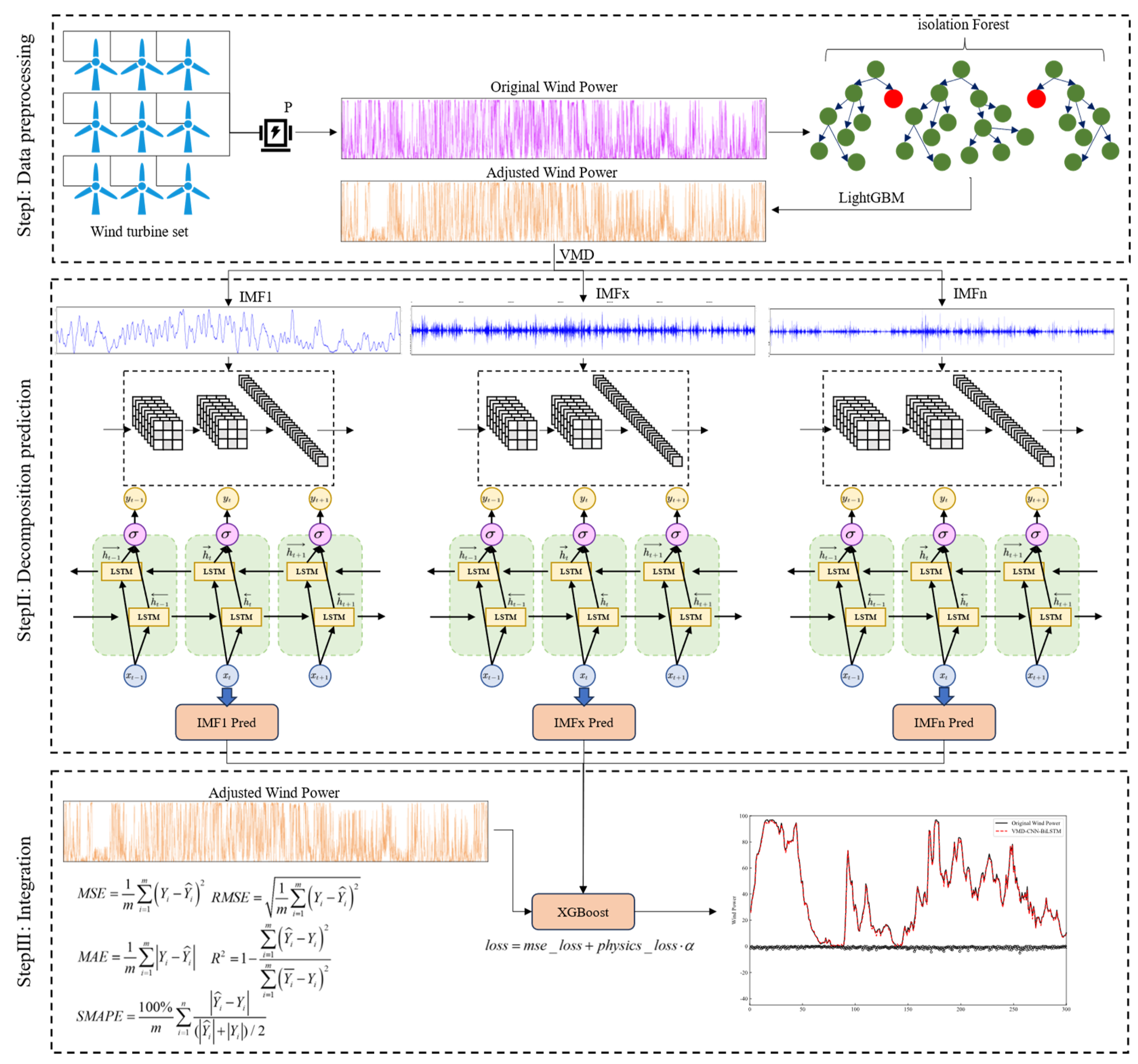
3. Proposed Method
3.1. Method Construction Process
3.2. Evaluation Metrics
4. Experimental Analysis
4.1. Data Description
4.2. Data Preprocessing
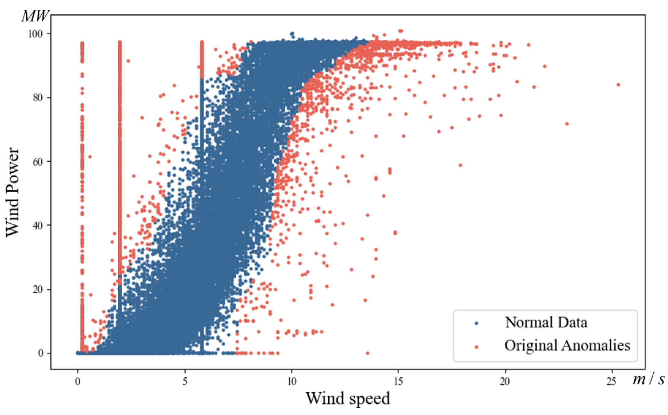
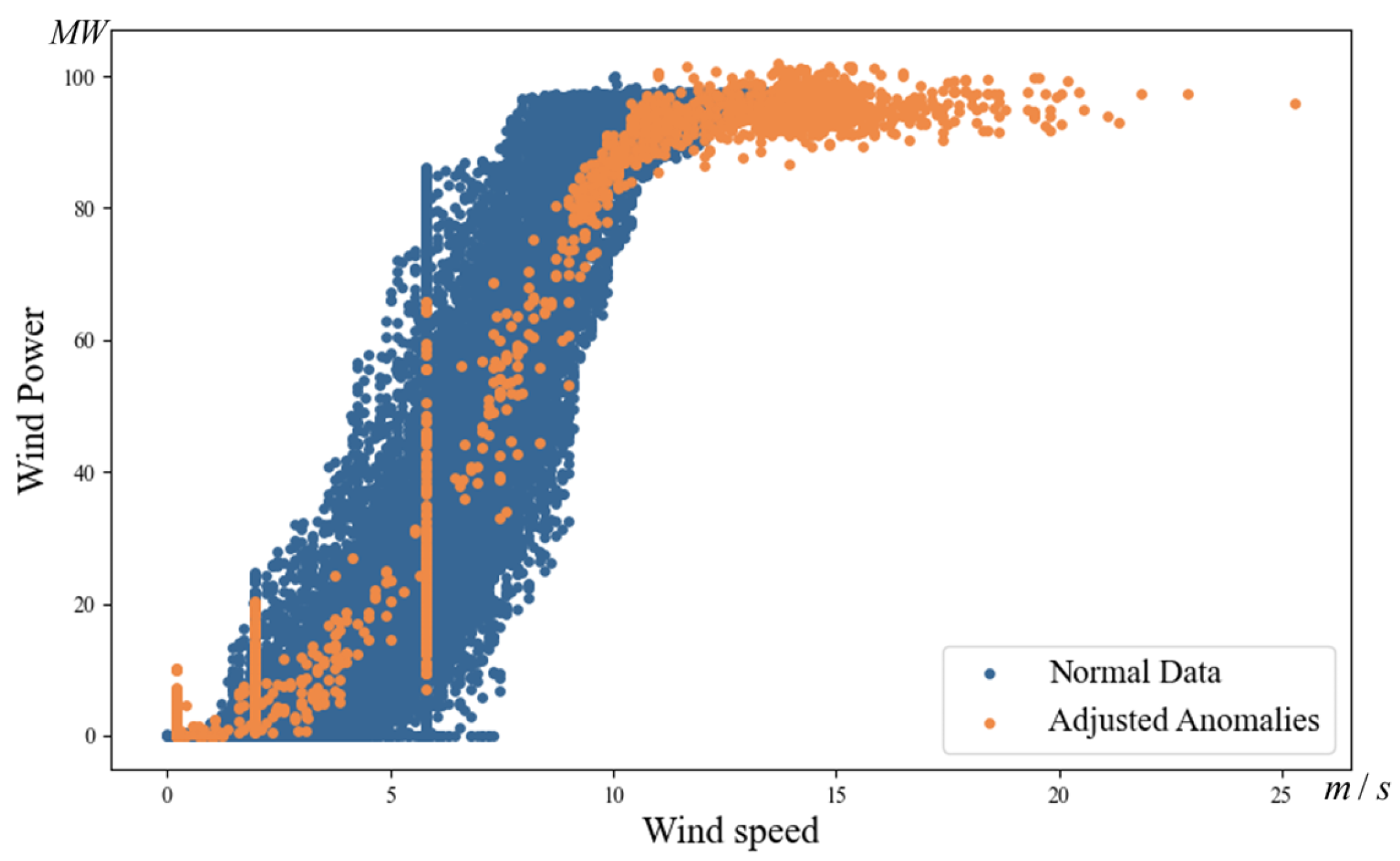
4.2.1. Outlier Repair
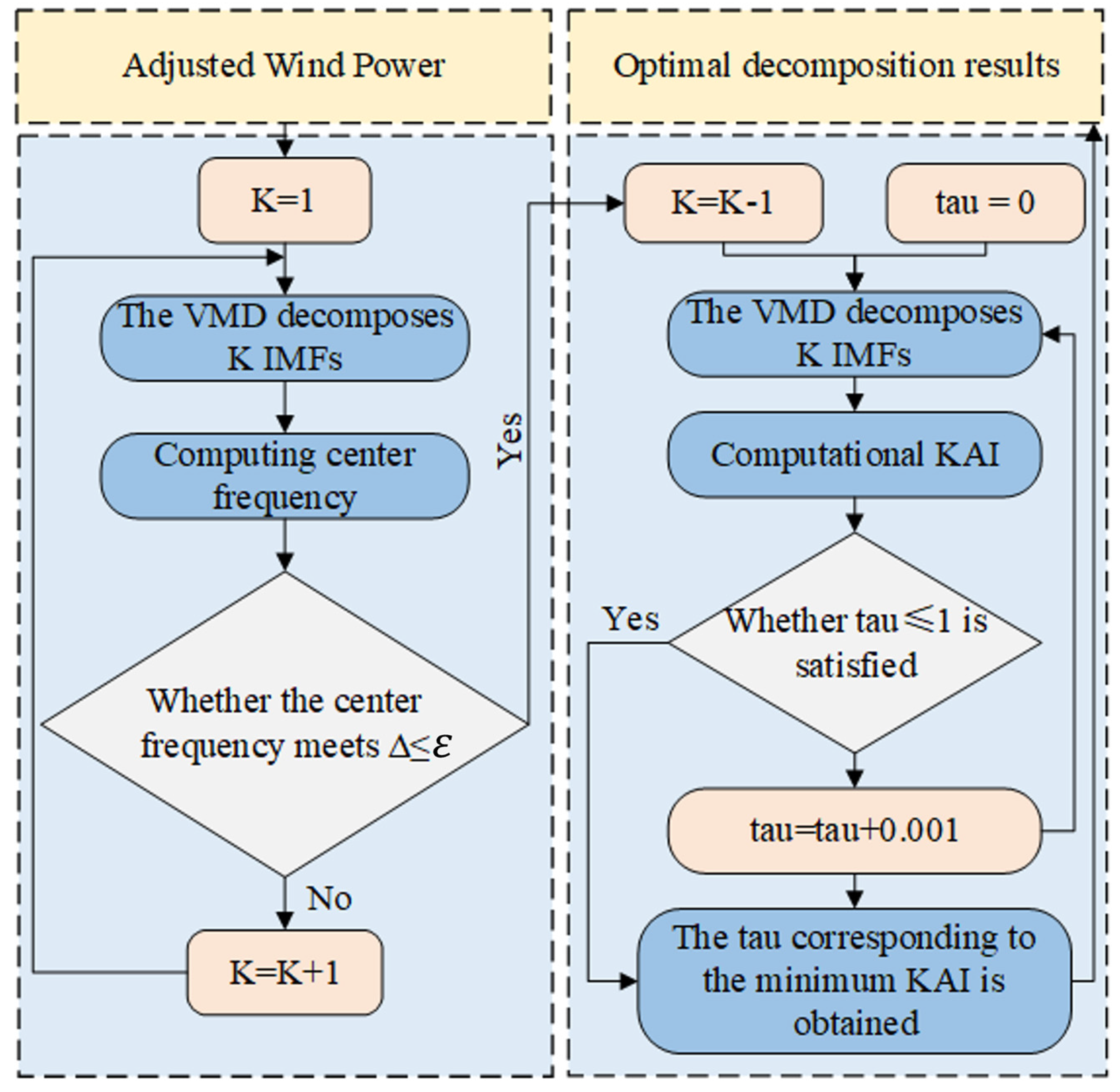
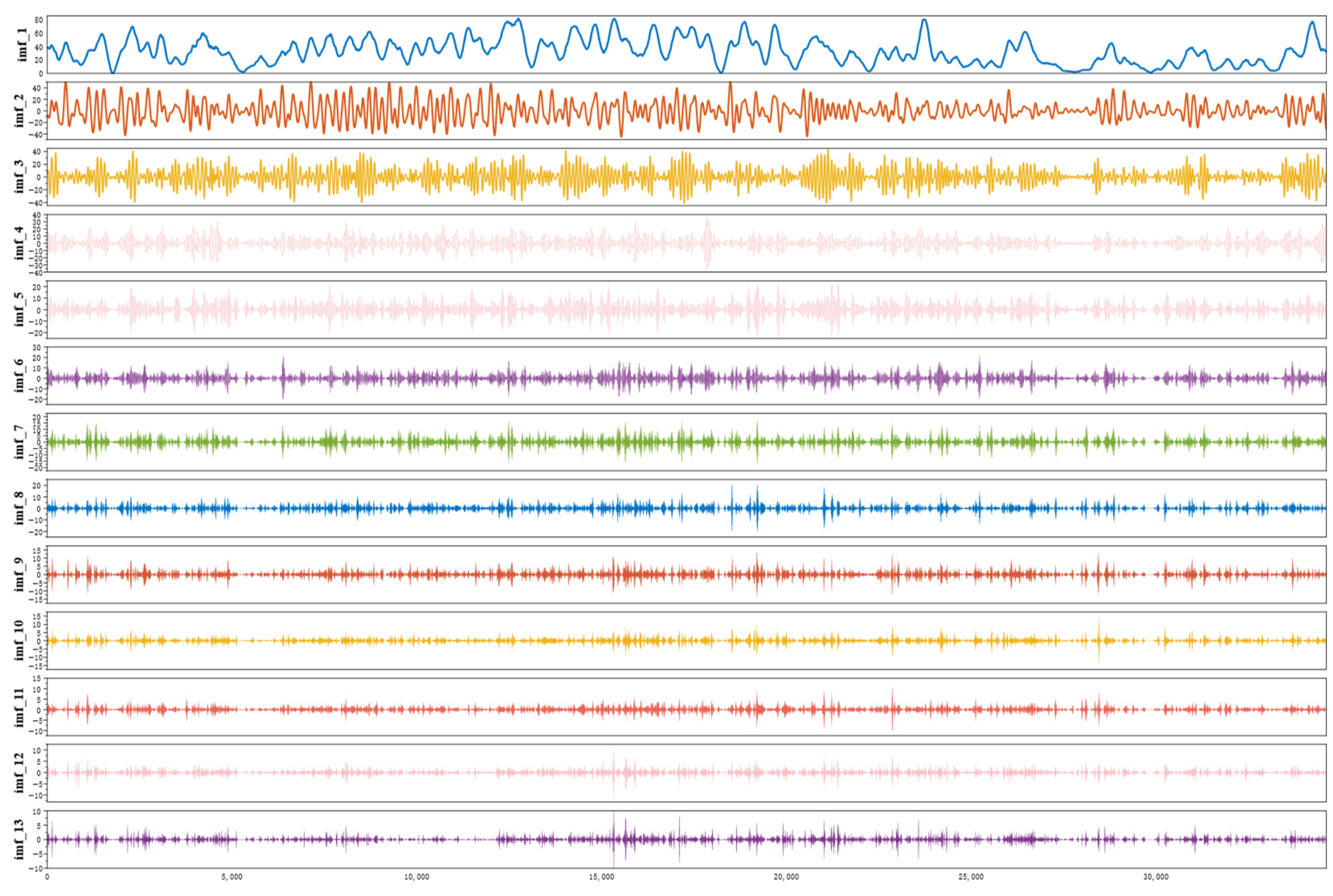
4.2.2. Data Decomposition
4.3. Parameter Setting of CNN-BiLSTM Prediction Method
4.4. Integration
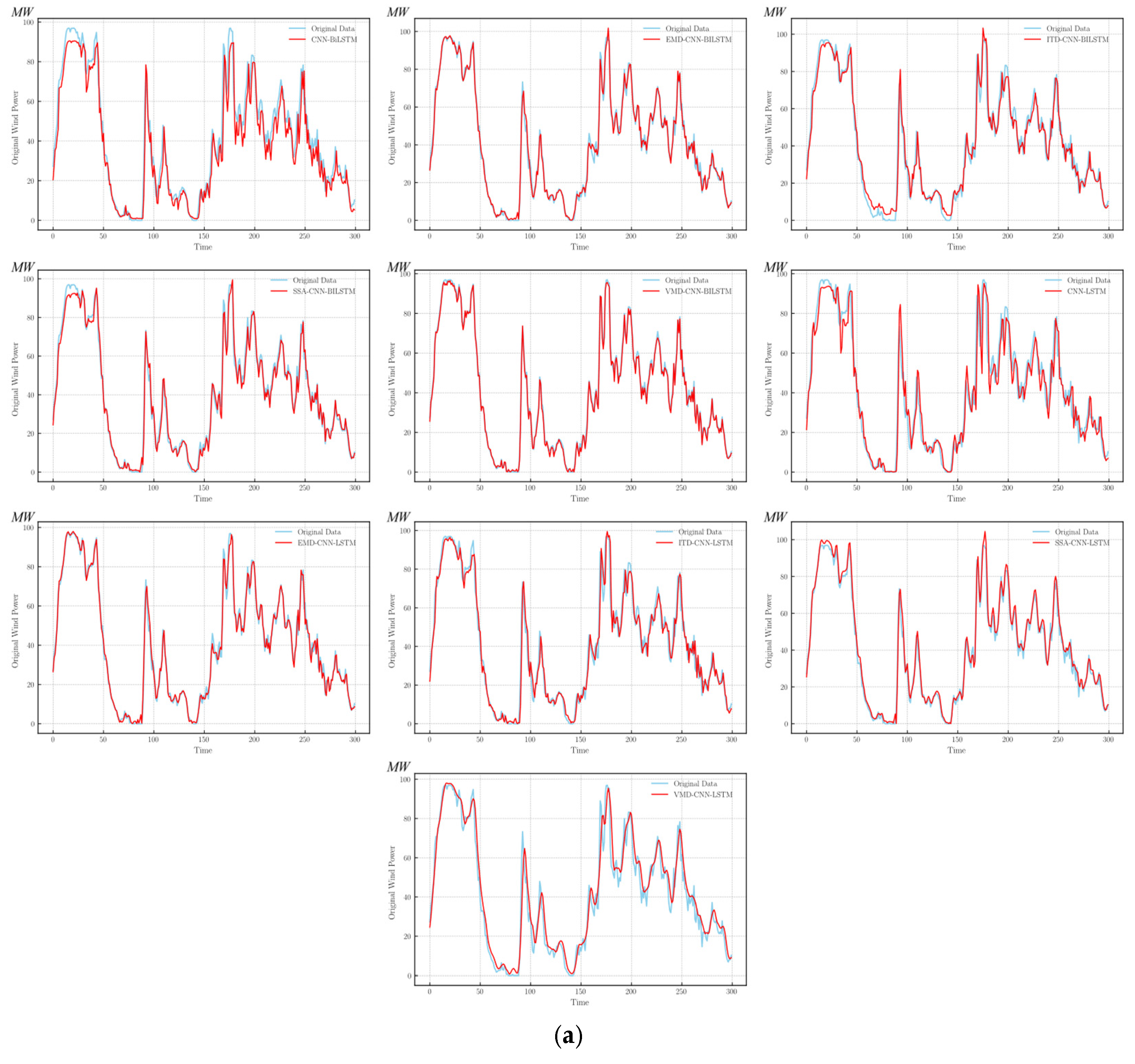
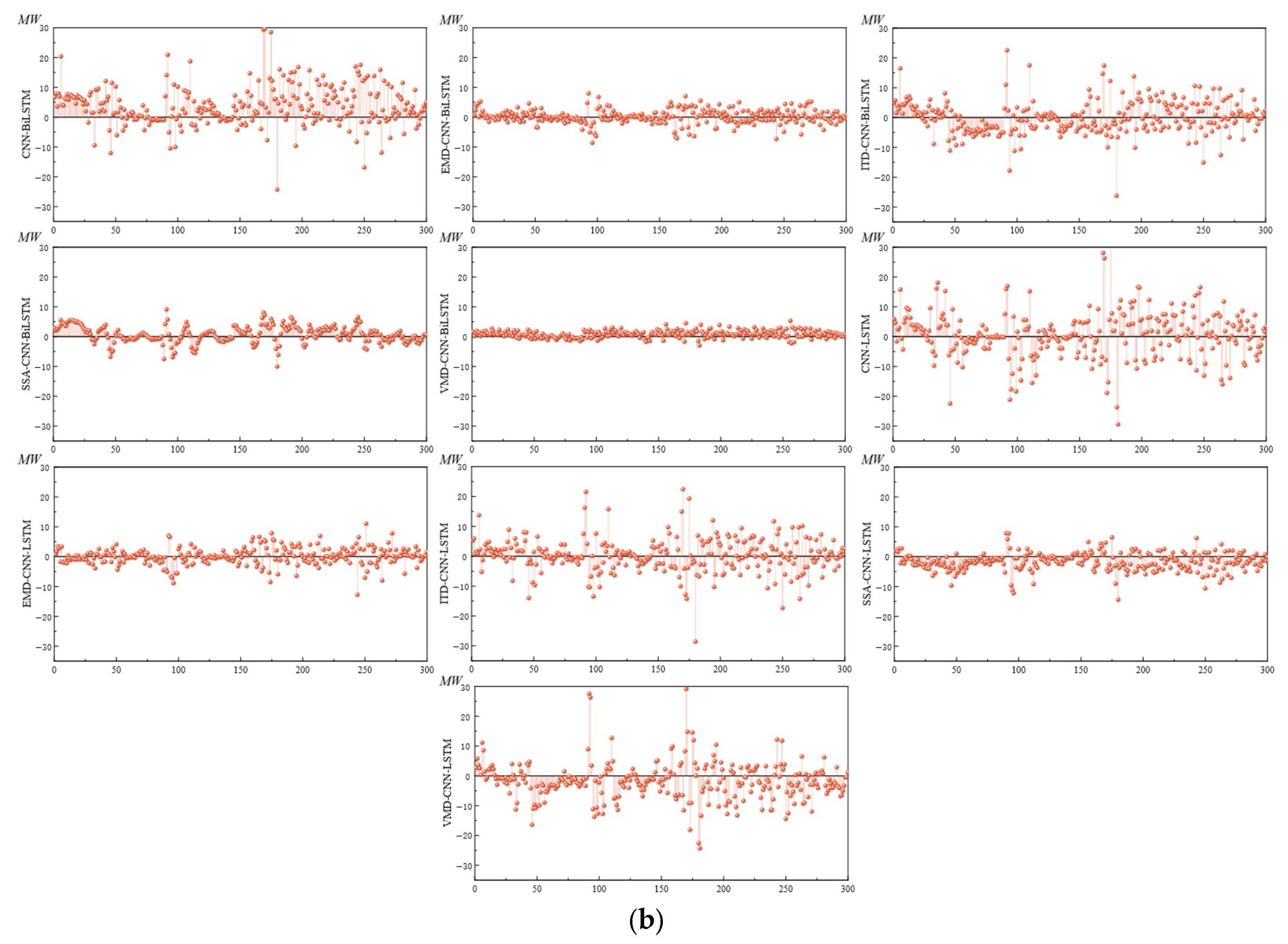
4.5. Method Comparison
5. Conclusions
Author Contributions
Funding
Institutional Review Board Statement
Informed Consent Statement
Data Availability Statement
Conflicts of Interest
References
- Chen, J.; Fu, X.; Zhang, L.; Shen, H.; Wu, J. A novel offshore wind power prediction model based on TCN-DANet-sparse transformer and considering spatio-temporal coupling in multiple wind farms. Energy 2024, 308, 132899. [Google Scholar] [CrossRef]
- Cheng, R.; Yang, D.; Liu, D.; Zhang, G. A reconstruction-based secondary decomposition-ensemble framework for wind power forecasting. Energy 2024, 308, 132895. [Google Scholar] [CrossRef]
- Yang, T.; Yang, Z.; Li, F.; Wang, H. A short-term wind power forecasting method based on multivariate signal decomposition and variable selection. Appl. Energy 2024, 360, 122759. [Google Scholar] [CrossRef]
- Zhu, J.; He, Y.; Yang, X.; Yang, S. Ultra-short-term wind power probabilistic forecasting based on an evolutionary non-crossing multi-output quantile regression deep neural network. Energy Convers. Manag. 2024, 301, 118062. [Google Scholar] [CrossRef]
- Wu, Y.H.; Wang, Y.S.; Xu, H.; Chen, Z.; Zhang, Z.; Guan, S.J. Survey of Wind Power Output Power Forecasting Technology. J. Front. Comput. Sci. Technol. 2022, 16, 2653–2677. [Google Scholar] [CrossRef]
- Cutler, N.J.; Outhred, H.R.; MacGill, I.F. Using nacelle-based wind speed observations to improve power curve modeling for wind power forecasting. Wind. Energy 2012, 15, 245–258. [Google Scholar] [CrossRef]
- Louka, P.; Galanis, G.; Siebert, N.; Kariniotaki, G.; Katsafados, P.; Pytharoulis, I.; Kallos, G. Improvements in wind speed forecasts for wind power prediction purposes using Kalman filtering. J. Wind Eng. Ind. Aerodyn. 2008, 96, 2348–2362. [Google Scholar] [CrossRef]
- Chen, N.; Sha, Q.; Tang, y.; Zhu, L.Z. A Conbination Method for Wind Power Predication Based on Cross Entropy Theory. Proc. CSEE 2012, 32, 29–34+22. [Google Scholar] [CrossRef]
- Huang, D.G.; Chen, Y.; Yang, Y. Wind Power Prediction in Complex Mountainous Region Based on Partition Modeling. Mod. Inf. Technol. 2023, 7, 162–165+170. [Google Scholar] [CrossRef]
- Gu, W.G.; Wang, F. Short-term wind power prediction based on BP optimized by an improved dung beetle optimization algorithm. J. Shanghai Dianji Univ. 2024, 27, 161–166+180. [Google Scholar] [CrossRef]
- Xue, Y.; Wang, L.; Wang, S.; Zhang, Y.F.; Zhang, N. An ultra-short-term wind power forecasting model combined with CNN and GRU networks. Renew. Energy Resour. 2019, 37, 456–462. [Google Scholar] [CrossRef]
- Han, L.; Jing, H.T.; Zhang, R.C.; Gao, Z.Y. Wind power forecast based on improved Long Short Term Memory network. Energy 2019, 189, 9. [Google Scholar] [CrossRef]
- Huang, F.; Li, Z.X.; Xiang, S.C.; Wang, R. A new wind power forecasting algorithm based on long short-term memory neural network. Int. Trans. Electr. Energy Syst. 2021, 31, 11. [Google Scholar] [CrossRef]
- Wang, L.J.; Dong, L.; Gao, s. Wind Power Short-term Prediction Based on Principal Component Analysis of NWP of Multiple Locations. Trans. China Electrotech. Soc. 2015, 30, 79–84. [Google Scholar] [CrossRef]
- Li, L.; Liu, Y.Q.; Yang, Y.P.; Han, S. Short-term Wind Speed Forecasting Based on CFD Pre-calculated Flow Fields. Proc. CSEE 2013, 33, 27–32. [Google Scholar] [CrossRef]
- An, X.; Jiang, D.; Zhao, M.; Liu, C. Short-term prediction of wind power using EMD and chaotic theory. Commun. Nonlinear Sci. Numer. Simul. 2011, 17, 1036–1042. [Google Scholar] [CrossRef]
- Zhang, X.; Wang, Q.; Niu, D.; Lai, K.K.; Zhang, Q. A Fuzzy Group Forecasting Model Based on Least Squares Support Vector Machine (LS-SVM) for Short-Term Wind Power %. J. Energ. 2012, 5, 3329–3346. [Google Scholar] [CrossRef]
- Wang, J.D.; Fang, K.J.; Pang, W.J.; Sun, J.W. Wind Power Interval Prediction Based on Improved PSO and BP Neural Network. J. Electr. Eng. Technol. 2017, 12, 989–995. [Google Scholar] [CrossRef]
- Zhu, J.P.; Wei, X.; Xie, L.R.; Yang, J.L. Short-Term Wind Power Peediction Based on Vmd and Improved Bilstm. Acta Energiae Solaris Sin. 2024, 45, 422–428. [Google Scholar] [CrossRef]
- Sun, H.B.; Cui, Q.; Wen, J.Y.; Kou, L.; Ke, W.D. Short-term wind power prediction method based on CEEMDAN-GWO-Bi-LSTM. Energy Rep. 2024, 11, 1487–1502. [Google Scholar] [CrossRef]
- Ding, Y.F.; Chen, Z.J.; Zhang, H.W.; Wang, X.; Guo, Y. A short-term wind power prediction model based on CEEMD and WOA-KELM. Renew. Energy 2022, 189, 188–198. [Google Scholar] [CrossRef]
- Abedinia, O.; Lotfi, M.; Bagheri, M.; Sobhani, B.; Shafie-khah, M.; Catalao, J.P.S. Improved EMD-Based Complex Prediction Model for Wind Power Forecasting. IEEE Trans. Sustain. Energy 2020, 11, 2790–2802. [Google Scholar] [CrossRef]
- Guo, Z.Y.; Wei, F.Z.; Qi, W.K.; Han, Q.L.; Liu, H.Y.; Feng, X.M.; Zhang, M.H. A Time Series Prediction Model for Wind Power Based on the Empirical Mode Decomposition-Convolutional Neural Network-Three-Dimensional Gated Neural Network. Sustainability 2024, 16, 3474. [Google Scholar] [CrossRef]
- Dragomiretskiy, K.; Zosso, D. Variational Mode Decomposition. IEEE Trans. Signal Process. 2014, 62, 531–544. [Google Scholar] [CrossRef]
- Sun, Y.; Zhou, Q.B.; Sun, L.; Sun, L.P.; Kang, J.C.; Li, H. CNN-LSTM-AM: A power prediction model for offshore wind turbines. Ocean Eng. 2024, 301, 15. [Google Scholar] [CrossRef]
- Hochreiter, S.; Schmidhuber, J. Long Short-Term Memory. Neural Comput. 1997, 9, 1735–1780. [Google Scholar] [CrossRef] [PubMed]
- Graves, A.; Schmidhuber, J. Framewise phoneme classification with bidirectional LSTM and other neural network architectures. Neural Netw. 2005, 18, 602–610. [Google Scholar] [CrossRef] [PubMed]
- Wan, A.; Peng, S.; Bukhaiti, K.A.; Ji, Y.; Ma, S.; Yao, F.; Ao, L. A novel hybrid BWO-BiLSTM-ATT framework for accurate offshore wind power prediction. Ocean Eng. 2024, 312, 119227. [Google Scholar] [CrossRef]
- Wen, T.X.; Xu, X.Y. Research on Image Perception of Tourist Destinations Based on the BERT-BiLSTM-CNN-Attention Model. Sustainability 2024, 16, 3464. [Google Scholar] [CrossRef]
- Tang, C.; Zhang, Y.F.; Wu, F.; Tang, Z. An Improved CNN-BILSTM Model for Power Load Prediction in Uncertain Power Systems. Energies 2024, 17, 2312. [Google Scholar] [CrossRef]
- Geng, D.H.; Wang, B.; Gao, Q. A hybrid photovoltaic/wind power prediction model based on Time2Vec, WDCNN and BiLSTM. Energy Convers. Manag. 2023, 291, 21. [Google Scholar] [CrossRef]
- Chen, T.; Guestrin, C. XGBoost: A Scalable Tree Boosting System. CoRR. arXiv 2016, arXiv:1603.02754. [Google Scholar]
- Chen, Y.; Xiao, J.W.; Wang, Y.W.; Luo, Y. Non-crossing quantile probabilistic forecasting of cluster wind power considering spatio-temporal correlation. Appl. Energy 2025, 377, 124356. [Google Scholar] [CrossRef]
- Yang, M.; Wang, D.; Zhang, W. A novel ultra short-term wind power prediction model based on double model coordination switching mechanism. Energy 2024, 289, 10. [Google Scholar] [CrossRef]
- Yu, G.Z.; Liu, C.Q.; Tang, B.; Chen, R.S.; Lu, L.; Cui, C.Y.; Hu, Y.; Shen, L.X.; Muyeen, S.M. Short term wind power prediction for regional wind farms based on spatial-temporal characteristic distribution. Renew. Energy 2022, 199, 599–612. [Google Scholar] [CrossRef]
- Yang, M.; Wang, D.; Xu, C.Y.; Dai, B.Z.; Ma, M.M.; Su, X. Power transfer characteristics in fluctuation partition algorithm for wind speed and its application to wind power forecasting. Renew. Energy 2023, 211, 582–594. [Google Scholar] [CrossRef]
- Liu, F.T.; Ting, K.M.; Zhou, Z.H. Isolation Forest. In Proceedings of the 2008 Eighth IEEE International Conference on Data Mining, Pisa, Italy, 15–19 December 2008. [Google Scholar]
- Huang, N.T.; Wu, Y.Y.; Cai, G.W.; Zhu, H.Y.; Yu, C.Y.; Jiang, L.; Zhang, Y.; Zhang, J.S.; Xing, E.K. Short-Term Wind Speed Forecast With Low Loss of Information Based on Feature Generation of OSVD. IEEE Access 2019, 7, 81027–81046. [Google Scholar] [CrossRef]
- Li, Q.; Ren, X.Y.; Zhang, F.; Gao, L.; Hao, B. A novel ultra-short-term wind power forecasting method based on TCN and Informer models. Comput. Electr. Eng. 2024, 120, 24. [Google Scholar] [CrossRef]
- Qu, K.; Si, G.Q.; Shan, Z.H.; Kong, X.G.; Yang, X. Short-term forecasting for multiple wind farms based on transformer model. Energy Rep. 2022, 8, 483–490. [Google Scholar] [CrossRef]

| Paper | Dataset | Method | Evaluation Metrics |
|---|---|---|---|
| Nicholas J.C. (2011) [6] | The Yambuk and Challicum Hills wind farms owned by Pacific Hydro Pty Ltd., the Bluff Point wind farm owned by Roaring40s Pty Ltd. | Wind farm power curve modeling | Root mean square error |
| Louka P. (2008) [7] | SKIRON NWP | F-NN, Kalman filtering | Absolute bias, standard deviation of the bias and of the absolute bias, root mean square error |
| Chen N. (2012) [8] | \ | Cross-entropy, ARIMA | Root mean square error |
| Huang D.G. (2023) [9] | A wind farm in Chongqing | KDE, BDE, SBL | PINAW, CWC |
| Gu W.G. (2024) [10] | \ | OLHS-DBO-BP | Mean square error, mean absolute error, symmetric mean absolute percentage error |
| Xue Y. (2019) [11] | Supervisory control and data acquisition | GRU, CNN | Mean square error |
| Han L. (2019) [12] | \ | VMD, ILSTM | Mean absolute percentage error |
| Huang F. (2021) [13] | \ | WPF | Mean absolute percentage error, mean square error, mean absolute error |
| Wang L.J. (2015) [14] | Heilongjiang Yilan wind farm | NWP | Root mean square error, mean absolute error |
| Li L. (2013) [15] | \ | CFD, NWP | \ |
| An X. L. (2012) [16] | Dongtai wind farm | EMD, GM(1,1) | Mean absolute percentage error, root mean square error, mean absolute error |
| Zhang Q. (2012) [17] | The Changshun wind park in Huade County, Inner Mongolia Autonomous Region, China | LS-SVM | Mean absolute percentage error |
| Wang J.D. (2017) [18] | Key Laboratory of Smart Grid of Ministry of Education (Tianjin University) | PSO-BP | PINAW, PICP |
| Sun H.B. (2024) [20] | A wind farm in Gansu Province | CEEMDAN-GWO-Bi-LSTM | Mean absolute percentage error, root mean square error, mean absolute error, R-squared |
| Guo Z.Y. (2024) [23] | Two wind farms in Xingtai, Hebei | EMD-CNN-TGNN | Root mean square error, mean square error, mean absolute error, R-squared |
| Date | Original Wind Speed | Original Wind Power |
|---|---|---|
| 1 November 2022 00:00:00 | 2.61 | 15.08 |
| 1 November 2022 00:15:00 | 5.54 | 18.73 |
| 1 November 2022 00:30:00 | 4.26 | 18.01 |
| 1 November 2022 00:45:00 | 2.86 | 18.38 |
| 1 November 2022 01:00:00 | 5.92 | 19.57 |
| 1 November 2022 01:15:00 | 6.05 | 16.63 |
| 1 November 2022 01:30:00 | 4.52 | 16.59 |
| 1 November 2022 01:45:00 | 6.05 | 19.59 |
| 1 November 2022 02:00:00 | 4.14 | 17.86 |
| 1 November 2022 02:15:00 | 6.56 | 19.2 |
| 1 November 2022 02:30:00 | 4.39 | 24.37 |
| …… | …… | …… |
| 19 February 2023 15:15:00 | 5.67 | 14.32 |
| 19 February 2023 15:30:00 | 4.52 | 13.93 |
| 19 February 2023 15:45:00 | 4.77 | 10.6 |
| 19 February 2023 16:00:00 | 5.79 | 10.55 |
| 19 February 2023 16:15:00 | 6.3 | 13.87 |
| …… | …… | …… |
| 28 July 2023 16:30:00 | 7.58 | 54.94 |
| 28 July 2023 16:45:00 | 6.3 | 32.85 |
| 28 July 2023 17:00:00 | 7.07 | 37.11 |
| 28 July 2023 17:15:00 | 6.17 | 35.37 |
| 28 July 2023 17:30:00 | 6.94 | 31.09 |
| 28 July 2023 17:45:00 | 6.3 | 38.19 |
| 28 July 2023 18:00:00 | 6.56 | 33.3 |
| 28 July 2023 18:15:00 | 5.41 | 33.27 |
| 28 July 2023 18:30:00 | 6.81 | 26.26 |
| 28 July 2023 18:45:00 | 4.26 | 11.45 |
| 28 July 2023 19:00:00 | 4.65 | 4.62 |
| …… | …… | …… |
| Method | Original Wind Power | Adjusted Wind Power |
|---|---|---|
| CNN-LSTM | 0.939120 | 0.952621 |
| CNN-BiLSTM | 0.943687 | 0.965677 |
| Decomposition Order | Center Frequency | Decomposition Order | Center Frequency |
|---|---|---|---|
| 1 | 0.001162 | 9 | 0.293598 |
| 2 | 0.028151 | 10 | 0.335073 |
| 3 | 0.06373 | 11 | 0.377056 |
| 4 | 0.090076 | 12 | 0.416864 |
| 5 | 0.129276 | 13 | 0.444295 |
| 6 | 0.164414 | 14 | 0.456638 |
| 7 | 0.210599 | 15 | 0.464797 |
| 8 | 0.251984 |
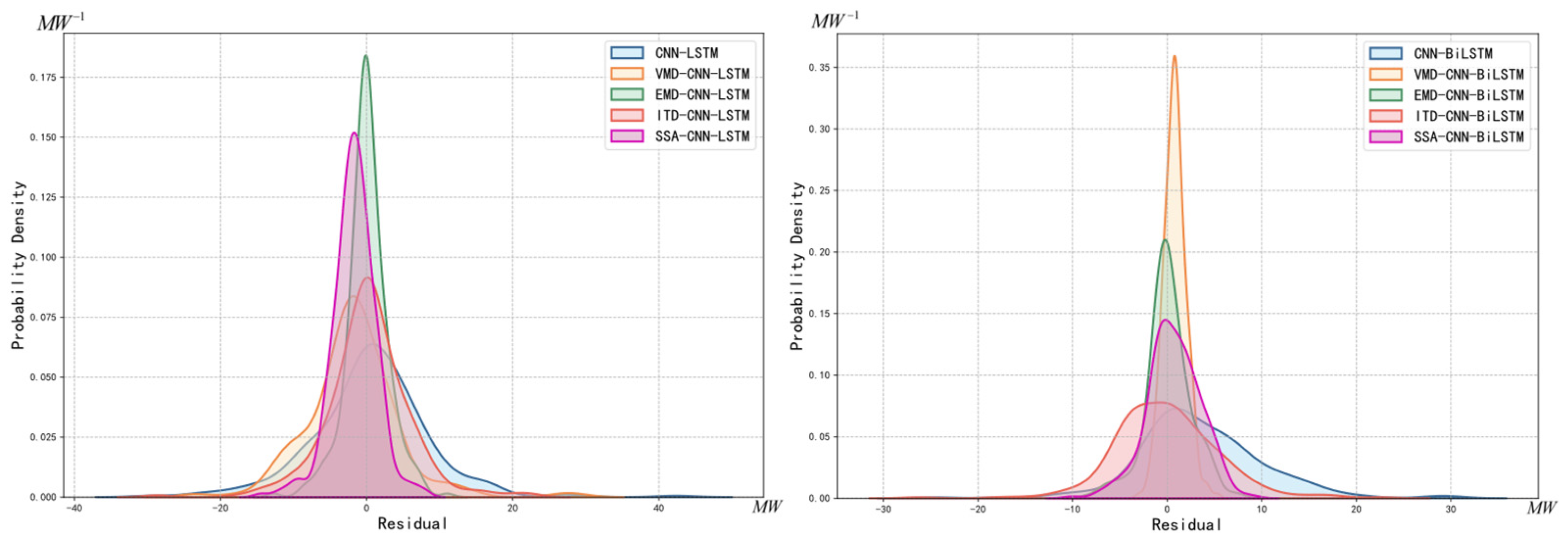
| Method | 90% Error Interval | 100% Error Interval |
|---|---|---|
| VMD-CNN-BiLSTM | [−1.1032,2.7440] | [−2.9589,5.3031] |
| VMD-CNN-LSTM | [−11.4684,8.2913] | [−24.3339,29.1793] |
| EMD-CNN-BiLSTM | [−4.0295,4.2888] | [−8.6179,7.9375] |
| EMD-CNN-LSTM | [−4.9226,4.7180] | [−12.7945,11.0244] |
| ITD-CNN-BiLSTM | [−7.3960,8.5354] | [−26.2526,22.5367] |
| ITD-CNN-LSTM | [−9.3298,8.8566] | [−28.6323,22.4461] |
| SSA-CNN-BiLSTM | [−4.1184,5.1928] | [−10.0490,9.1120] |
| SSA-CNN-LSTM | [−6.2855,2.5584] | [−14.4681,7.8608] |
| CNN-BiLSTM | [−4.8532,14.6923] | [−24.3245,29.5787] |
| CNN-LSTM | [−12.5328,12.3496] | [−29.4859,42.3572] |
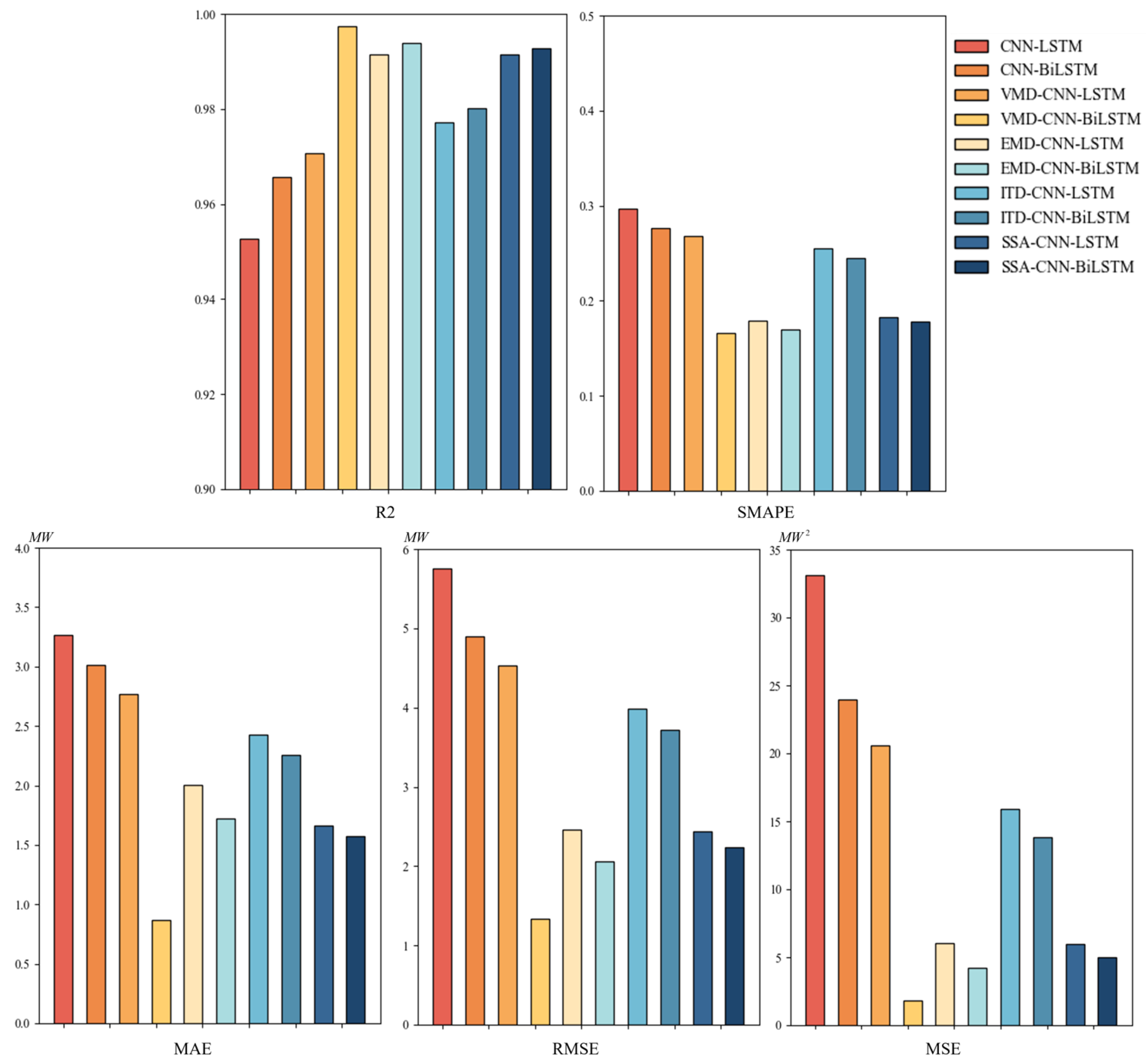
| Method | R2 | MSE | RMSE | MAE | SMAPE |
|---|---|---|---|---|---|
| VMD-CNN-BiLSTM | 0.997436 | 1.7924 | 1.3388 | 0.8691 | 16.63% |
| VMD-CNN-LSTM | 0.970595 | 20.5535 | 4.5336 | 2.7648 | 26.80% |
| ITD-CNN-BiLSTM | 0.980177 | 13.8562 | 3.7224 | 2.2579 | 24.45% |
| ITD-CNN-LSTM | 0.977234 | 15.9133 | 3.9891 | 2.4284 | 25.51% |
| EMD-CNN-BiLSTM | 0.993964 | 4.2189 | 2.054 | 1.7184 | 16.96% |
| EMD-CNN-LSTM | 0.99138 | 6.0251 | 2.4546 | 2.0065 | 17.94% |
| SSA-CNN-BiLSTM | 0.992849 | 4.9988 | 2.2358 | 1.5743 | 17.80% |
| SSA-CNN-LSTM | 0.991464 | 5.9664 | 2.4426 | 1.6608 | 18.28% |
| CNN-BiLSTM | 0.965677 | 23.9912 | 4.8981 | 3.0155 | 27.66% |
| CNN-LSTM | 0.952621 | 33.1168 | 5.7572 | 3.2669 | 29.68% |
| VMD-TCN-Informer [39] | 0.994 | / | / | / | / |
| Transformer [40] | 0.939 | / | / | / | / |
| Data Processing Method | CNN-LSTM | CNN-BiLSTM |
|---|---|---|
| VMD | 143 s | 158 s |
| ITD | 390 s | 455 s |
| EMD | 327 s | 382 s |
| SSA | 171 s | 279 s |
| Do not Decomposition | 127 s | 146 s |
Disclaimer/Publisher’s Note: The statements, opinions and data contained in all publications are solely those of the individual author(s) and contributor(s) and not of MDPI and/or the editor(s). MDPI and/or the editor(s) disclaim responsibility for any injury to people or property resulting from any ideas, methods, instructions or products referred to in the content. |
© 2025 by the authors. Licensee MDPI, Basel, Switzerland. This article is an open access article distributed under the terms and conditions of the Creative Commons Attribution (CC BY) license (https://creativecommons.org/licenses/by/4.0/).
Share and Cite
Liu, Y.; Gu, Y.; Long, Y.; Zhang, Q.; Zhang, Y.; Zhou, X. Research on Physically Constrained VMD-CNN-BiLSTM Wind Power Prediction. Sustainability 2025, 17, 1058. https://doi.org/10.3390/su17031058
Liu Y, Gu Y, Long Y, Zhang Q, Zhang Y, Zhou X. Research on Physically Constrained VMD-CNN-BiLSTM Wind Power Prediction. Sustainability. 2025; 17(3):1058. https://doi.org/10.3390/su17031058
Chicago/Turabian StyleLiu, Yongkang, Yi Gu, Yuwei Long, Qinyu Zhang, Yonggang Zhang, and Xu Zhou. 2025. "Research on Physically Constrained VMD-CNN-BiLSTM Wind Power Prediction" Sustainability 17, no. 3: 1058. https://doi.org/10.3390/su17031058
APA StyleLiu, Y., Gu, Y., Long, Y., Zhang, Q., Zhang, Y., & Zhou, X. (2025). Research on Physically Constrained VMD-CNN-BiLSTM Wind Power Prediction. Sustainability, 17(3), 1058. https://doi.org/10.3390/su17031058