Optimal Operation Strategy of Virtual Power Plant Using Electric Vehicle Agent-Based Model Considering Operational Profitability

Abstract

Growing EV adoption is reshaping how Distributed Energy Resources (DERs) interact with the grid, playing a pivotal role in global decarbonization efforts and the transition towards a sustainable energy future. This study built a Virtual Power Plant (VPP) operation framework centered on EV behavioral dynamics, connecting individual driving and charging behaviors with the physical and economic layers of energy management. The EV behavioral dynamic model quantifies the stochastic travel, parking, and charging behaviors of individual EVs through an Agent-Based Trip and Charging Chain (AB-TCC) simulation, producing a Behavioral Flexibility Trace (BFT) that represents time-resolved EV availability and flexibility. The Forecasting Model employs a Bi-directional Long Short-Term Memory (Bi-LSTM) network trained on historical meteorological data to predict short-term renewable generation and represent physical variability. The two-stage optimization model integrates behavioral and physical information with market price signals to coordinate day-ahead scheduling and real-time operation, minimizing procurement costs and mitigating imbalance penalties. Simulation results indicate that the proposed framework yielded an approximately 15% increase in revenue over 7 days through EV-based flexibility utilization. These findings demonstrate that the proposed approach effectively leverages EV flexibility to manage renewable generation variability, thereby enhancing both the profitability and operational reliability of VPPs in local distribution systems. This facilitates greater penetration of intermittent renewable energy sources, accelerating the transition to a low-carbon energy system.

1. Introduction

The global shift toward low-carbon energy is transforming how modern power systems are built and operated. As centralized generation dominated by fossil fuels gives way to Distributed Energy Resources (DERs) such as solar panels, wind turbines, and Electric Vehicles (EVs), the grid is becoming fragmented and dynamic. While these technologies are essential for decarbonization and fostering an environmentally sustainable future, their variability adds layers of operational complexity. Temporal and spatial fluctuations in their generation and demand profiles complicate real-time coordination and system balancing. In response, the concept of a virtual power plant (VPP) has emerged as a promising mechanism to coordinate and operate DERs as a single controllable entity capable of market participation and grid support provision [1,2].

In the changing energy landscape, electric vehicles (EVs) take on two complementary roles. They increase demand on the grid as a rapidly expanding electrical load, yet they also act as distributed storage that can discharge power to the grid through Vehicle-to-Grid (V2G). When aggregated, EV fleets can charge surplus renewable energy or discharge power during peak demand to the gird, improving reliability and cost efficiency [3]. This dynamic capability enhances resource utilization and contributes to the circular economy principles within the energy sector, fostering a more sustainable and resilient energy infrastructure. The operational use of EV flexibility is still constrained. Unlike stationary energy storage units, EVs are subject to behavioral factors in that when and how long EVs can charge or discharge depends on the driver’s travel routine, parking duration, and range anxiety.

Capturing this uncertainty driven by behavior is essential for integrating EVs into system level decision frameworks such as VPP operation. However, most operational models continue to represent EV behavior through static or deterministic assumptions. Although research on EV integration has expanded rapidly, most operational studies represent EV behavior through static or deterministic assumptions, such as fixed charging times, fixed locations, or uniform driving distances [4]. These simplifications reduce computational complexity but undermine the realism required for short-term operational analysis. Many studies have adopted stochastic or scenario-based models to account for behavioral uncertainty [5], yet they typically depend on home centered parameters such as average departure and arrival times or daily mileage. This approach overlooks spatial diversity, trip chaining, and the interdependence between consecutive charging events. EVs move among various locations, such as home, workplace, shopping area, commercial, and recreational area, and each stop changes the chance of being connected to the grid. When these travel sequences are ignored, inaccurate estimation of available flexibility can be misjudged. The flexibility information is critically needed by VPPs for effective scheduling.

Previous studies have provided valuable insights into the coordination of virtual power plants, yet most existing models still oversimplify the behavioral dynamics of electric vehicles. A multi time scale scheduling framework based on deferrable loads treated EVs merely as shiftable demand and did not account for mobility or behavioral uncertainty [6]. A risk averse scheduling framework for VPP operation under uncertain market conditions failed to capture the real-time connection variability of mobile resources such as EVs [7]. The coordination of wind generation and aggregated EV charging ignored spatial and temporal diversity in charging behavior [8]. Capacity allocation and power dispatching formulations assumed fixed EV availability windows and overlooked the heterogeneity of charging activities across time and location [9,10]. Multi objective dispatching under the V2G mode relied on a static single period formulation that could not represent dynamic EV flexibility [11]. Stochastic robust optimization effectively addressed renewable and price uncertainty but excluded user behavior and mobility variability [12]. Recent advances in EV integration into VPP scheduling incorporated cluster level representations and heuristic algorithms, yet they continued to depend on fixed or nighttime only charging assumptions without probabilistic representations of individual mobility patterns [13,14].

Many studies assume EV flexibility to be a fixed parameter, yet in reality, it depends significantly on the drivers’ travel patterns, parking duration, and charging preferences. The uncertainty arising from these behavioral factors remains a challenge for operational optimization. The absence of behavior dependent input limits the accuracy of flexibility estimation and reduces the practical relevance of optimization outcomes. To address these challenges, this study proposes an EV behavioral dynamic-driven virtual power plant operation framework that integrates behavioral, physical, and economic dimensions within a unified data-driven structure. The proposed framework consists of three interconnected models: (1) an EV Behavioral Dynamics Model that models the stochastic evolution of EV travel, parking, and charging behaviors through an agent-based trip and charging chain (AB-TCC) simulation, and converts the resulting behavioral states into a Behavioral Flexibility Trace (BFT) that quantifies the time-resolved availability and flexibility of individual EVs; (2) a Forecasting Model that employs a Bi-directional Long Short-Term Memory (Bi-LSTM) network trained on historical meteorological data to predict short-term renewable generation, thereby capturing physical variability in wind power; and (3) a Two-stage Optimization Model that coordinates day-ahead scheduling and real-time operation using market price signals, renewable forecasts, and behaviorally derived flexibility information.

In the day-ahead (DA) stage, the optimization model shifts controllable EV charging sessions toward low-price hours to minimize procurement costs while keeping schedules behaviorally and technically feasible. In the real-time (RT) stage, the optimization model updates dispatch every five minutes to correct forecast errors and respond to price fluctuations. The system’s layered coordination improves both cost efficiency and operational stability. By aligning behavioral variability with physical and market uncertainties, it allows the control structure to adapt smoothly to changing conditions. This adaptive capacity is crucial for the long-term viability and sustainability of decentralized energy systems, enabling a more reliable and cost-effective integration of renewables. The integration of BFT data enables the VPP to operate based on the actual temporal and spatial flexibility of EV fleets, rather than relying on static or assumed charging profiles.

The main contributions of this study are summarized as follows.

(1)

It introduces a behavior-aware operational approach that quantifies EV behavioral dynamics and translates them into real-time flexibility indicators via the BFT, establishing a direct connection between human mobility patterns and system operation.

(2)

It develops a unified data-driven framework combining behavioral simulation, renewable forecasting, and two-stage optimization for realistic VPP coordination under uncertainty.

(3)

It demonstrates, through an integrated simulation using empirical travel data, ERA5 meteorological data, and market prices, that the proposed approach enhances both profitability and operational stability by leveraging EV-based flexibility.

The remainder of this paper is organized as follows. Section 2 presents the proposed modeling framework and its three integrated modules. Section 3 provides the case study and numerical results. Finally, Section 4 concludes the study and discusses future research directions.

2. Modeling Framework

The proposed framework, as illustrated in Figure 1, integrates three interconnected models that collectively represent the behavioral, physical, and economic dimensions of VPP operation. The EV Behavioral Dynamics Model quantifies the behavioral uncertainty of EVs through the AB-TCC model, generating a Behavioral Flexibility Trace (BFT) that describes the time-resolved availability and flexibility of individual EVs. The Forecasting Model employs a Bi-LSTM network trained on historical meteorological data to predict short-term renewable generation, thereby modeling the physical variability of the system. The Two-stage Optimization Model integrates behavioral flexibility and renewable forecasts into a unified scheduling structure. It performs day-ahead cost minimization based on predicted wind generation and market prices and real-time re-dispatch using the optimization to mitigate imbalance penalties and operational deviations. Collectively, these three models form a behaviorally and physically informed decision-making architecture that enhances the profitability and operational reliability of VPP under renewable and market uncertainty.

2.1. AB-TCC Model

2.1.1. Trip Data and Probability Distributions

The trip and charging chain (AB-TCC) model was constructed using empirical mobility statistics derived from the 2022 U.S. National Household Travel Survey (NHTS) [15]. The NHTS provides detailed household-level travel diaries that record departure and arrival times, trip purposes, travel distances, durations, and transportation modes for both weekdays and weekends. Based on these data, a set of empirical probability distributions, collectively denoted as $\mathcal{P},$ was developed to represent the stochastic patterns of daily travel behavior. Each probability represents an empirically observed relationship among time of day, location, travel mode, distance, and dwell duration.

The complete parameter set used in the AB-TCC model is defined as:

$$\mathcal{P}=\left\{P\right(T_d,p_d),P(p_e\mid T_d,p_d),P(u\mid T_d,p_d,p_e),f(d\mid p_d,p_e,u),P(t_p\mid T_d,p_e\left)\right\}$$

(1)

where $P(T_d,p_d)$ denotes the joint probability of departure time and origin type, $P(p_e\mid T_d,p_d)$ represents the conditional transition probability from origin $p_d$ to destination $p_e$ given the departure time, $P(u\mid T_d,p_d,p_e)$ is the conditional probability of EV use, reflecting the likelihood that a trip between $(p_d,p_e)$ at time $T_d$ is taken by an EV, $f(d\mid p_d,p_e,u)$ defines the log-normal probability density function of trip distance conditioned on origin, destination, and EV use, and $P(t_p\mid T_d,p_e)$ denotes the conditional dwell time distribution at the destination and time of day.

Each probability component in Equation (1) is directly estimated from the NHTS dataset and stored as a discrete lookup table. During the simulation, each EV agent sequentially selects trip attributes including departure time, origin, destination, trip distance, and dwell duration based on these probability tables, forming individual trip chains without additional parameter estimation. Separate sets of probability tables are constructed for weekdays and weekends to reflect temporal variations in mobility behavior. These empirical distributions constitute the stochastic foundation of the AB-TCC model, enabling each EV agent to generate realistic trip chains that reproduce the observed daily travel patterns while preserving heterogeneity across individuals.

2.1.2. Trip and Charging Chain Generation

Each EV agent generates a chain of travel and charging activities over an entire day, guided by the probabilistic parameters defined in $\mathcal{P}$.

The $n$-th trip of agent $i$ is represented by the state vector

$$S_{i,n}=(p_{d,n},T_{d,n},d_n,t_n,p_{e,n},t_{p,n})$$

(2)

where $p_{d,n}$ and $p_{e,n}$ denote the origin and destination zones, $T_{d,n}$ is the departure time, $d_n$ is the trip distance, $t_n$ is the travel time, and $t_{p,n}$ is the dwell duration at the destination. At each step, these variables are probabilistically chosen from the empirical distributions in Equation (1).

After completing each trip, the next trip starts at

$$T_{d,n+1}=T_{d,n}+t_n+t_{p,n},p_{d,n+1}=p_{e,n}$$

(3)

If no EV use is selected, the agent remains parked for the dwell duration, representing non-driving periods.

During travel, the agent’s SOC, $s_i\left(t\right)$, decreases according to its efficiency $e_i$ and battery capacity $E_{cap,i}$:

$$s_i\left(t+∆t\right)=s_i\left(t\right)-{\displaystyle \frac{e_i{d}_n}{E_{cap,i}}}$$

(4)

Upon arrival, if $s_i\left(t\right)$ falls below the agent’s predefined preferred charging threshold $s_i^{pref}$, charging is initiated. Simply, the model adopts a constant charging rate based on charging power profiles that indicate a stable power level [16].

Charging continues until SOC reaches the upper limit $s_i^{max}$ or the available dwell time expires.

The SOC evolution during charging follows

$$s_i\left(t+∆t\right)=\mathrm{m}\mathrm{i}\mathrm{n}(s_i^{max},s_i\left(t\right)+{\displaystyle \frac{{\eta }^{chg}{P}^{chg}(t)∆t}{E_{cap,i}}}),$$

(5)

where $P^{chg}\left(t\right)$ is the instantaneous charging power bounded by both on board charger and the site’s rated capacity, and ${\eta }^{chg}$ denotes charging efficiency.

Through this recursive process, each EV agent cycles through driving, parking, and charging, forming a complete trip and charging chain across the simulation period.

2.1.3. Aggregated Outputs and Behavioral Flexibility Trace

The simulation records each EV’s driving, parking, and charging status at one minute resolution, from which binary indicators and power limits for V2G usability are derived. Let $\tau$ denote the minute level time index, and define the state of agent $i$ as

$$X_i\left(\tau \right)=\{lo{c}_i\left(\tau \right),s_i\left(\tau \right),ac{t}_i\left(\tau \right)\},$$

(6)

where $lo{c}_i\left(\tau \right)$ denotes the current location, $s_i\left(\tau \right)$ the SOC, and $ac{t}_i\left(\tau \right)\in \{drive,park,charge\}$ the current state.

For each minute $\tau$, a binary availability flag $a_i\left(\tau \right)$ is defined as

$$a_i\left(\tau \right)=\left\{\begin{array}{c}1,iftheEViseligibleforV2Goperations\hfill \\ 0,otherwise\hfill \end{array}\right..$$

(7)

Specifically, $a_i\left(\tau \right)$ is 1 when the EV is parked, charging is possible ($s_i\left(\tau \right)<s_i^{max}$) or, discharging is possible $s_i\left(\tau \right)>s_i^{min}$; and remaining parking time exceeds 5 min ($∆t_{remain}\left(\tau \right)>5)$. The instantaneous charging or discharging power of agent $i$ is constrained within operational limits as

$$\underset{¯}{P_i}\left(\tau \right)\le P_i\left(\tau \right)\le \overline{P_i}\left(\tau \right),$$

(8)

which ensures that the SOC remains within its upper and lower bounds during each time step. These minute-level time series are subsequently aligned with the temporal resolution of the VPP optimization stage, where aggregated behavioral information from all agents is used to define flexibility bounds and availability constraints. The behavioral indicators generated from the AB-TCC simulation offer realistic, data-driven inputs that reflect the spatial, temporal, and behavioral diversity of EV fleets within the integrated VPP framework. BFT reflects two forms of EV flexibility. The first is unidirectional load shifting that is applied in the day-ahead stage, where charging demand can be shifted across time. The second is bidirectional V2G flexibility that is activated in the real-time stage, allowing for both charging and discharging depending on the system and market conditions.

2.2. Wind Forecasting Model

2.2.1. Spatio-Temporal Structure and Dataset

Wind and meteorological variables were obtained from ERA5 reanalysis data provided by the Copernicus Climate Data Store (CDS) [17].

The grid location $l$ is identified by latitude ${\varphi }_l$, and longitude ${\lambda }_l$, and $t$ represents the hourly UTC time index. The ERA 5 single level meteorological variables at each ($t$, $l$) are expressed as

$$x_{t,l}={\left(u10,v10,td2,t2m,sp,ssrd,tcc,cdir,fdir,ssrdc\right)}_{t,l},$$

(9)

where $u10$ and $v10$ are the 10 m wind components, $td2$ and $t2m$ are the 2 m dewpoint and air temperature, $sp$ is surface pressure, $ssrd$ and $ssrdc$ are total and clear-sky downward short-wave radiation, $tcc$ is total cloud cover, and $cdir$ and $fdir$ are direct and diffuse radiation components.

The prediction target is the one hour ahead 10 m wind speed,

$$y_{t,l}=ws{10}_{t,l}=\sqrt{u{10}_{t,l}^2+v{10}_{t,l}^2},$$

(10)

where $ws{10}_{t,l}$ represents the magnitude of the horizontal wind vector at each location and time. The model generates a one-hour-ahead forecast using a sliding input window that includes the most recent observations.

2.2.2. Feature Engineering

The wind direction ${\theta }_{t,l}$ is calculated as

$${\theta }_{t,l}=\mathrm{d}\mathrm{e}\mathrm{g}\left[\arctan 2\left(-u{10}_{t,l},-v{10}_{t,l}\right)\right],$$

(11)

and its cyclic characteristics are represented through sine and cosine transformations:

$$\sin \left({\theta }_{t,l}\right)=\sin ({\theta }_{t,l}\pi /180),\cos \left({\theta }_{t,l}\right)=\cos ({\theta }_{t,l}\pi /180)$$

(12)

where these trigonometric encodings enable the model to capture directional periodicity.

Thermal-humidity and air-density proxies are formulated as

$$td{d}_{t,l}=t2m_{t,l}-td{2}_{t,l},{\rho }_{t,l}^{proxy}={\displaystyle \frac{s{p}_{t,l}}{Rt2m_{t,l}}},$$

(13)

where $td{d}_{t,l}$ is the temperature-dewpoint difference approximating relative humidity, ${\rho }_{t,l}^{proxy}$ is a proxy for air density, and $R$ is the gas constant for dry air that is 287.05.

To represent radiative and sky conditions, the following ratio are defined:

$$clearsk{y}_{t,l}={\displaystyle \frac{ssr{d}_{t,l}}{ssrd{c}_{t,l}+\epsilon }},{dirfrac}_{t,l}={\displaystyle \frac{{fdir}_{t,l}}{{ssrd}_{t,l}+\epsilon }},{dirclr}_{t,l}={\displaystyle \frac{{cdir}_{t,l}}{{ssrdc}_{t,l}+\epsilon }}$$

(14)

where $\epsilon$ prevents division overflow that is ${10}^{-6}$.

$clearsky$ indicates the ratio of observed to clear-sky radiation, $dirfrac$ represents the fraction of direct radiation under total radiation, and $dirclr$ denotes the direct clear-sky ratio.

Hourly and annual periodicity are introduced as

$$\begin{gathered} h_{sin}(t)=\sin \left(2\pi {\displaystyle \frac{h\left(t\right)}{24}}\right),h_{cos}(t)=\cos \left(2\pi {\displaystyle \frac{h\left(t\right)}{24}}\right), \\ {d}_{sin}(t)=\sin \left(2\pi {\displaystyle \frac{d\left(t\right)}{366}}\right),d_{cos}(t)=\cos \left(2\pi {\displaystyle \frac{d\left(t\right)}{366}}\right), \end{gathered}$$

(15)

where $h\left(t\right)$ is the hour of the day and $d\left(t\right)$ is the day of the year.

These cyclic encodings allow the network to recognize daily and seasonal periodicity in wind patterns.

2.2.3. Data Preprocessing and Sequence Formation

The training period covered 2021 to 2023, and the testing period was from 4 June to 10 June in 2024. All input features and target values were standardized with respect to the training period mean and standard deviation to ensure consistent scaling and prevent data leakage:

$${\widehat{x}}_{t,l}={\displaystyle \frac{{\tilde{x}}_{t,l}-{\mu }_{tr}^x}{{\sigma }_{tr}^x}},{\widehat{y}}_{t,l}={\displaystyle \frac{y_{t,l}-{\mu }_{tr}^x}{{\sigma }_{tr}^y}},$$

(16)

A lookback window covering the past 48 h, equivalent to approximately two days, was applied to construct time series samples. For each time step t, the model input and target are defined as:

$$x_{t,l}=[{\widehat{x}}_{t-48,l},{\widehat{x}}_{t-47,l},\dots ,{\widehat{x}}_{t-1,l}],y_{t,l}={\widehat{y}}_{t,l}$$

(17)

The last portion of the training data, corresponding to about 15% of all samples in chronological order, is reserved for validation. To enhance generalization, a correlation-based feature selection was applied using Pearson correlation computed on the training dataset. Variables with a correlation magnitude above 0.15 were retained, while physically significant features such as wind components, temperature difference, and time-based cyclic terms were always included. This selection process minimizes redundancy and improves model interpretability.

2.2.4. Model Architecture and Training Configuration

Each input sequence $x_{t,l}$ is processed by a Bi-LSTM network designed to capture both short-term and long-term dependencies in wind dynamics. The model includes a Gaussian noise layer for regularization, a Bi-LSTM layer that processes temporal context in both directions, a dropout layer to prevent overfitting, and a fully connected dense layer with ReLU activation and $L_2$ regularization. The output layer generates a single continuous prediction of standardized wind speed. The Huber loss function, combined with $L_2$ penalties, is used to balance sensitivity and robustness against outliers. Model optimization is performed using the Adam algorithm with adaptive learning rate scheduling and early stopping based on validation loss. The best-performing model is selected according to minimum validation error while maintaining the chronological order of all training samples.

2.2.5. Forecasting, Evaluation, and Rationale

During testing, the model performs one step ahead rolling forecasts by using the most recent input window for each prediction. Forecasted values are reconstructed from standardized outputs using the training statistics, and negative wind speeds are truncated to zero. This single step rolling design prevents recursive error accumulation and reflects the operational nature of short-term wind forecasting. The predicted 10 m wind speeds were extrapolated to the turbine hub height by applying the logarithmic wind-profile law, which accounts for surface roughness on vertical wind shear:

$${\widehat{v}}_{hub,t,l}={\widehat{ws10}}_{t,l}\times {\displaystyle \frac{\mathrm{l}\mathrm{n}(H_l/z_{0,l})}{\mathrm{l}\mathrm{n}(10/z_{0,l})}}$$

(18)

where $z_{0,l}$ represents the local surface roughness length obtained from ERA5 data, and $H_l$ denotes the hub height of the turbine installed at location $l$. The logarithmic ratio ${\displaystyle \frac{\mathrm{l}\mathrm{n}(H_l/z_{0,l})}{\mathrm{l}\mathrm{n}(10/z_{0,l})}}$ scales the 10 m reference wind speed to the turbine hub height, effectively accounting for terrain-dependent aerodynamic drag. For physical consistency, $z_{0,l}$ is limited to between 0.001 m to 5 m, which represent smooth water surfaces and rough urban terrains, respectively.

Once the hub-height wind speed is determined, the instantaneous power output of each turbine is calculated according to its manufacturer power curve, which defines electrical generation as a function of wind speed. This curve is governed by three characteristics speed thresholds, which are the cut-in speed ($v_{cin,l})$, the rated speed ($v_{rated,l})$ and the cut-out speed ($v_{cout,l})$. A piecewise function can be expressed as follows:

$${\widehat{P}}_{t,l}=\left\{\begin{array}{c}0,v_{hub,t,l}<v_{cin,l},\\ f_l,v_{cin,l}\le {\widehat{v}}_{hub,t,l}<v_{rated,l},\\ P_{rated,l},v_{rated,l}\le {\widehat{v}}_{hub,t,l}\le v_{cout,l},\\ 0,{\widehat{v}}_{hub,t,l}>v_{cout,l},\end{array}\right.$$

(19)

where $f_l$ represents the interpolated power curve obtained from manufacturer data, which is implemented via linear interpolation between measured wind power pairs. When wind speed is below the cut-in threshold, the turbine stays idle. Between the cut-in and rated speeds, its output rises nonlinearly, reaching a cap at the rated capacity $P_{rated,l}$. Beyond the cut-out point, the turbine shuts down automatically to prevent mechanical damage.

The model’s performance is evaluated using mean absolute error (MAE) and normalized mean absolute error (NMAE):

$$MA{E}_l={\displaystyle \frac{1}{T_{test}}}\sum |{\widehat{y}}_{t,l}-y_{t,l}|,NMA{E}_l={\displaystyle \frac{MA{E}_l}{P_{rated,l}}}\times 100\%$$

(20)

where $P_{rated,l}$ denotes the rated capacity of wind turbine installed at location $l$.

The forecasting model combines several design choices intended to balance realism and robustness. Its scale-independent evaluation allows for a fair comparison among locations with different wind patterns, and the single rolling step inference keeps errors from accumulating over time. The bidirectional network captures both daily variations and broader seasonal cycles, while the Huber loss and regularization terms reduce the model’s sensitivity to outliers. By selecting the most informative predictors, the framework remains stable, providing a sound basis for the optimization stage.

2.3. Two-Stage VPP Optimization Model

2.3.1. Day-Ahead Optimization

In the DA stage, the optimization reallocates charging power within each parked session identified by the AB-TCC model. Each session corresponds to a continuous parking period during which charging is physically possible. The objective is to shift the charging load within the session toward hours with lower day-ahead market prices, thereby minimizing total charging cost while ensuring that every EV’s daily power requirement is satisfied. Let the hourly set $T_d=\{1,2,\dots ,24\}$ represent the 24-hourly intervals of day $d$, and $S_d$, denotes the set of all parked sessions available on that day. For each session $(i,s)$ belonging to agent $i$, the decision variable $x_{i,s,t}$ represents the amount of charging power allocated to hour $t$.

The problem is formulated as a linear program:

$$\begin{gathered} \underset{x}{\min }\sum _{t\in T_d}{\pi }_t\sum _{(i,s)\in S_d}{x}_{i,s,t} \\ \mathrm{s}.\mathrm{t}.0\le x_{i,s,t}\le {\overline{C}}_{i,s,t},\forall \left(i,s,t\right)\in S_d\times T_d, \\ \sum _{t\in T_d}{x}_{i,s,t}=P_{i,s}^{req},\forall \left(i,s\right)\in S_d \end{gathered}$$

(21)

where ${\pi }_t$ is the day-ahead LMP trend, ${\overline{C}}_{i,s,t}$ denotes the maximum charging capacity available for session $\left(i,s\right)$ during hour $t$, and $P_{i,s}^{req}$ represents the total power requirement to fully charge the EV at the beginning of the session. The day-ahead LMP trend is constructed using a second-order Fourier series fitted to the 2024 hourly day-ahead LMP historical data. The first constraint ensures that the scheduled charging does not exceed the available capacity during each hour, while the second enforces that the total charging energy per session equals the required power. The model keeps the total daily charging demand unchanged but redistributes power toward lower-priced hours, reshaping its temporal pattern. This shift moves charging events to cheaper periods within each parking window, cutting costs while keeping physical feasibility intact. Any unmet charging amount is carried over to the next day’s session as $∆P_{i,s}=P_{i,s}^{req}-{\sum }_t{x}_{i,s,t}$ ensuring continuity across rolling horizons. The resulting day-ahead schedule forms the baseline for the real-time optimization stage.

2.3.2. Real-Time Optimization

In the RT stage, an optimization model is applied to compensate for renewable generation deviations and to utilize short-term flexibility from EVs. The optimization operates on a five-minute timescale, solving a mixed-integer linear programming (MILP) problem at each control step. At every time step, the most recent wind power deviation and real-time price signals are incorporated as inputs. The first control action is implemented, and the optimization horizon is then shifted forward by one slot in a receding-horizon fashion. In this framework, a slot refers to the basic 5 min control interval, a session represents a continuous parking period while charging or discharging can occur, and a segment denotes a subset of slots within a session used to maintain intra session power neutrality. These concepts link the behavioral layer and the operational layer, allowing the system to preserve individual EV constraints while coordinating aggregate flexibility.

Let the set of 5 min slots within the day be denoted as $T=\{s_0,s_1,\dots ,s_{287}\}$, and at time step $k$ be represented by $T_k=\left\{s_k\right\}$. For each available EV agent $i$ and slot $s\in T_k$ binary decision variables $y_{i,s}^{+}$ and $y_{i,s}^{-}$ indicate whether the agent is charging or discharging, respectively.

The total power contribution from EV agent i at slot s is defined as:

$$H_s={\sum }_i{P}^{slot}(y_{i,s}^{+}-y_{i,s}^{-}),$$

(22)

where $P^{slot}=Q/12$ represents the power corresponding to the rated power $Q$ for a 5-min interval.

The WT forecast and observation at the hourly level are denoted by $P_t$ and $O_t$, respectively. $P_t$ and $O_t$ are expanded to 5-min resolution so that, for each slot $s$, a symmetric $\pm$10% prediction band is obtained.

$$L_s=0.9P_s,U_s=1.1P_s$$

(23)

To allow occasional band violations, a nonnegative slack variable ${\zeta }_s\ge 0$ is introduced, and the EV aggregation $H_s$ is constrained so that the net WT power after controlling EVs,

$${\tilde{O}}_s=O_s-H_s,$$

(24)

remains inside the relaxed band:

$$L_s-{\zeta }_s\le {\tilde{O}}_s\le U_s+{\zeta }_s.$$

(25)

Let $R{T}_s$ and $D{A}_s$ denote the RT and DA LMPs that converted to 5-min resolution and $c^{deg}$ be the battery degradation cost. The battery degradation cost is set at 0.0023 $/kWh, which is derived based on a weighted Ah-throughput model that applies a constant degradation cost factor, as described in [18]. In addition, ${\theta }_s$ represents an activation threshold, which is charged once per charging and discharging action through an activation cost $c_s^{act}={\theta }_s{P}^{slot}$. To encourage neutral power behavior at both the individual and session level, the model includes auxiliary slack variables ${\eta }_i^{+},{\eta }_i^{-}\ge 0$ for in the symmetric band EV agent-level neutrality of charging and discharging power and ${\xi }_s\ge 0$ for tail zone throughput relaxation, with associated penalty weights ${\lambda }_{neu}{\lambda }_{band}$ and ${\lambda }_{tail}$.

The RT stage minimizes the following objective at step $k$ expressed as:

$$\begin{gathered} \min \sum _{s\in T_k}\left(R{T}_s-D{A}_s\right)(-H_s)+c^{deg}\sum _{s\in T_k}{P}^{slot}(y_{i,s}^{+}+y_{i,s}^{-}) \\ +\sum _{s\in T_k}{c}_s^{act}\sum _i(y_{i,s}^{+}+y_{i,s}^{-})+{\lambda }_{band}\sum _{s\in T_k}{\zeta }_s+{\lambda }_{neu}\sum _i({\eta }_i^{+}+{\eta }_i^{-}) \\ +{\lambda }_{tail}\sum _{s\in T_k}{\xi }_s \end{gathered}$$

(26)

where the first term quantifies the settlement impact of using EVs to compensate for wind forecast errors, while the remaining terms penalize battery degradation, activation frequency, band violations, and residual imbalances at both the agent and session levels.

The following constraints are imposed.

Each EV can either charge, discharge, or keep idle in a slot:

$$y_{i,s}^{+}+y_{i,s}^{-}\le 1,y_{i,s}^{+},y_{i,s}^{-}\in \left\{0,1\right\},\forall i,s\in T_k.$$

(27)

To avoid uneconomic actions, charge and discharge are only allowed when the RT LMP is sufficiently above or below a symmetric activation threshold that accounts for degradation:

$$\left\{\begin{array}{c}R{T}_s\le D{A}_s+{\theta }_s+c^{deg}\Rightarrow y_{i,s}^{+}=0,\\ R{T}_s\ge D{A}_s-\left({\theta }_s+c^{deg}\right)\Rightarrow y_{i,s}^{-}=0,\end{array}\right.\forall i,s\in T_k.$$

(28)

The aggregated EV power must keep the wind output within the relaxed prediction band:

$$L_s-O_s-{\zeta }_s\le H_s\le U_s-O_s+{\zeta }_s,{\zeta }_s\ge 0.$$

(29)

The DA optimization allocates a minimum number of usable 5-min slots per EV agent and hour to satisfy the uncontrolled charging requirement. The remaining 5-min positions in that hour can be used for RT flexibility. Let $N_{i,h}^{allow}$ denote the maximum number of RT charging and discharging activations allowed to the DA schedule.

$$\sum _{s\in T_k:h\left(s\right)=h}\left(y_{i,s}^{+}+y_{i,s}^{-}\right)\le N_{i,h}^{allow},\forall i,h.$$

(30)

which preserves the integrity of the DA schedule and avoids excessive cycling in a single hour.

To discourage systematic charging or discharging bias at the individual level, the model considers, for each agent $i$, a subset $T_{i,k}^{neu}\in T_k$ of recent in-band slots in which at least one charge or discharge is activated, and RT capacity remains. Let $c_i^{past}$ denote the net energy previously committed by agent $i$ up to step $k$. The following neutrality constraint is imposed:

$$\sum _{s\in T_{i,k}^{neu}}{h}_{i,s}+c_i^{past}={\eta }_i^{+}+{\eta }_i^{-},{\eta }_i^{+},{\eta }_i^{-}\ge 0,\forall i.$$

(31)

which avoids affecting each EV agent’s trip pattern.

Each continuous parking segment $\sigma$ of agent $i$ is decomposed into consecutive slots, and the last part of the segment is designated as its tail zone. Let $\{s_{\sigma ,1},\dots ,s_{\sigma ,k_{\sigma }}\}$ be the ordered tail slots for segment $\sigma$, and let $c_{\sigma }^{past}$ be the cumulative net energy of that segment up to the start of the tail. For each tail slot, a recursive residual variable is defined:

$$H_{\sigma ,0}=c_{\sigma }^{past},R_{\sigma ,j}=R_{\sigma ,j-1}+\sum _{i\in \sigma }{h}_{i,s_{\sigma },j},j=1,\dots ,k_{\sigma }$$

(32)

A binary sigh variable $z_{\sigma ,j}\in \{0,1\}$ indicates the sign of the previous residual $R_{\sigma ,j-1}$ and enforces that each tail action reduces the magnitude of the residual. Tail actions always push the segment imbalance back toward zero and are bounded by the physical slot capacity.

$$\left\{\begin{array}{c}{z}_{\sigma ,j}=1\Rightarrow R_{\sigma ,j-1}\ge 0,h_{i,s_{\sigma ,j}}\in \left[-P^{slot},0\right],\\ z_{\sigma ,j}=0\Rightarrow R_{\sigma ,j-1}\le 0,h_{i,s_{\sigma ,j}}\in \left[0,P^{slot}\right],\hfill \end{array}\right.j=1,\dots ,k_{\sigma }.$$

(33)

If all tail slots of the segment are contained in the current horizon, the residual is forced to zero at the end of the tail.

At each step $k$, the optimization problem is solved using the latest LMP, wind forecast band, and EV session availability from DA stage. Only the first control action $\{y_{i,s_k}^{+},y_{i,s_k}^{-}\}$ is executed, and the horizon then shifts forward by one slot and cumulative residuals $(c_i^{past},c_{\sigma }^{past})$ are updated. Through this iterative process, the RT optimization continually tracks wind forecast errors within a probabilistic band, exploits profitable price spreads, and maintains both fleet-level and session-level neutrality with the physical constraints of individual EV sessions.

3. Case Study and Numerical Results

This section evaluates the performance of the proposed model through case studies based on simulation experiments. All models were implemented in Python 3.10 using Tensorflow 2.15, mesa 2.1, and Pyomo 6.6 with the Gurobi 12.0.3 solver. The proposed framework was executed on a PC equipped with an Intel Core i9-12900k processor at 3.2 GHz and 128 GB of RAM. The simulation scenario included an aggregation of 10,000 EVs to assess scalability under large-scale operational conditions. Under this setting, the average computation time was 51.3 s, which meets the real-time requirements of a 5 min operational cycle, confirming that the proposed scheduling framework is feasible for practical VPP operation.

3.1. Simulation Setup and Data Description

The AB-TCC model was calibrated using empirical travel statistics from the 2022 NHTS, which provides detailed records of departure and arrival times and locations, travel distance, and dwell duration. Additionally, the distribution of registered EV models in Colorado was incorporated to represent the composition of the simulated fleet [19]. The synthetic EV fleet comprised 24 commercially available models, shown in Figure 2, with battery capacities of 40–170 kWh and efficiencies between 2.0 and 4.1 miles/kWh, proportionally weighted by U.S. market shares to capture realistic fleet-level energy behavior. Furthermore, the preferred SOC threshold for initiating charging was determined based on a survey of EV drivers in South Korea, reflecting real-world charging preferences and behavioral tendencies. Using these parameters, a synthetic fleet of 10,000 EV agents was then simulated over a period of 7 days at one minute resolution, producing time series data of driving, parking, and charging states along with the SOC trajectory for each EV. Fleet level charging and availability profiles aggregated from the AB-TCC simulation were subsequently converted into BFT, which served as flexibility boundaries for the VPP optimization stage.

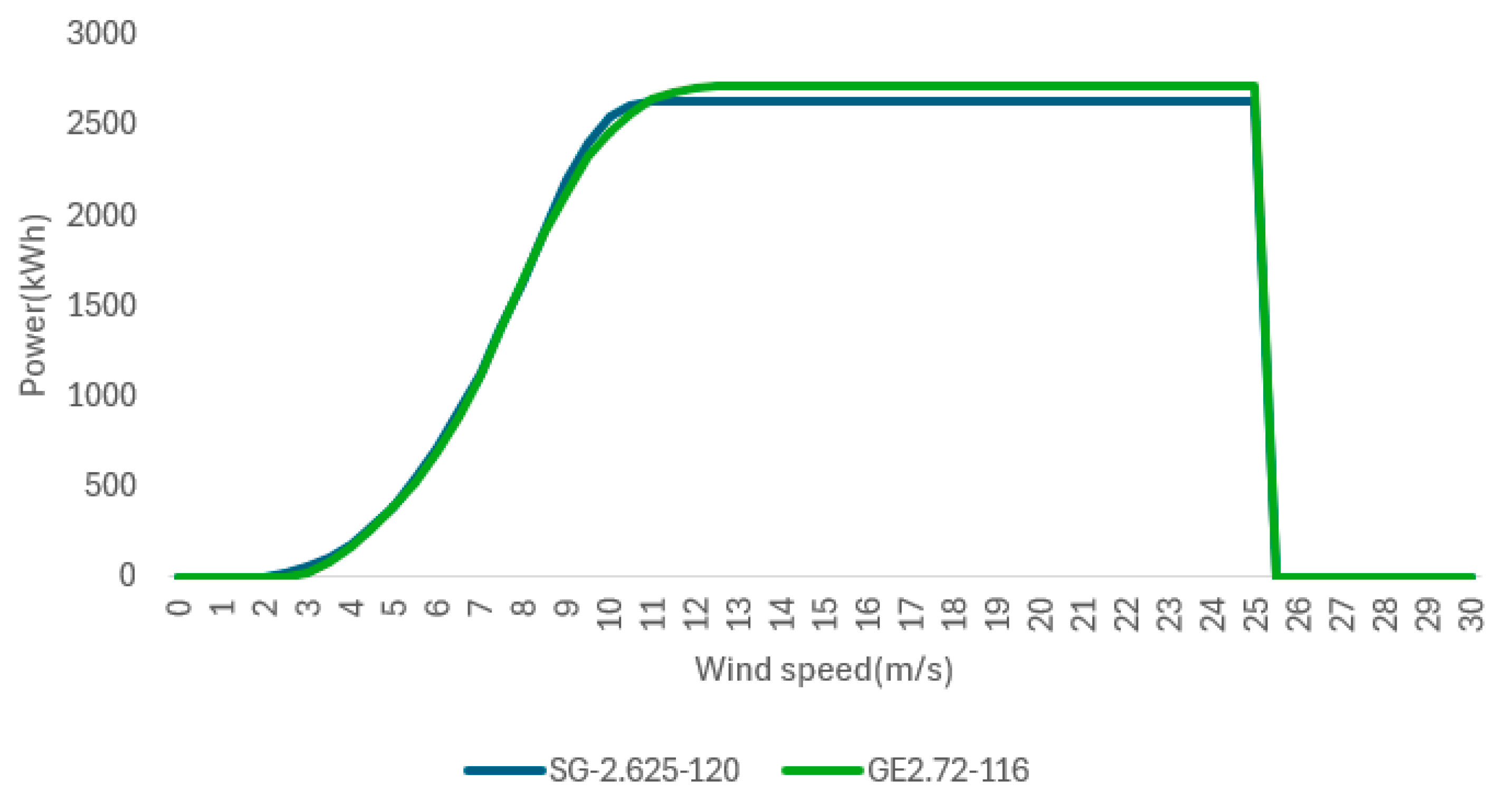
The wind forecasting model was trained using ERA5 hourly reanalysis data from 2021 to 2023, covering the region between 39.0–39.5° N and 101.5–100.9° W, and evaluated on data from 4 June to 10 June in 2024. Wind speeds were converted to equivalent power outputs using turbine specifications from the U.S. Wind Turbine Database (USWTDB) [20]. The representative power curve of the two turbines is shown in Figure 3, while their technical parameters, including rated capacity, hub height, rotor diameter, and swept area, are summarized in

Table 1. Technical specifications of the turbines.

Turbine Model	Capacity (kW)	Hub Heigh (m)t	Rotor Diameter (m)	Rotor Swept Area (m2)	Total Height (m)
SG-2.625-120	2625	85	120	11,309.73	145.1
GE2.72-116	2720	90	116	10,568.32	148.1

. For the case study, the installed wind capacity consists of two SG-2.625-120 turbines and four GE 2.72-116 turbines, resulting in a total installed capacity of 15,940 kW.

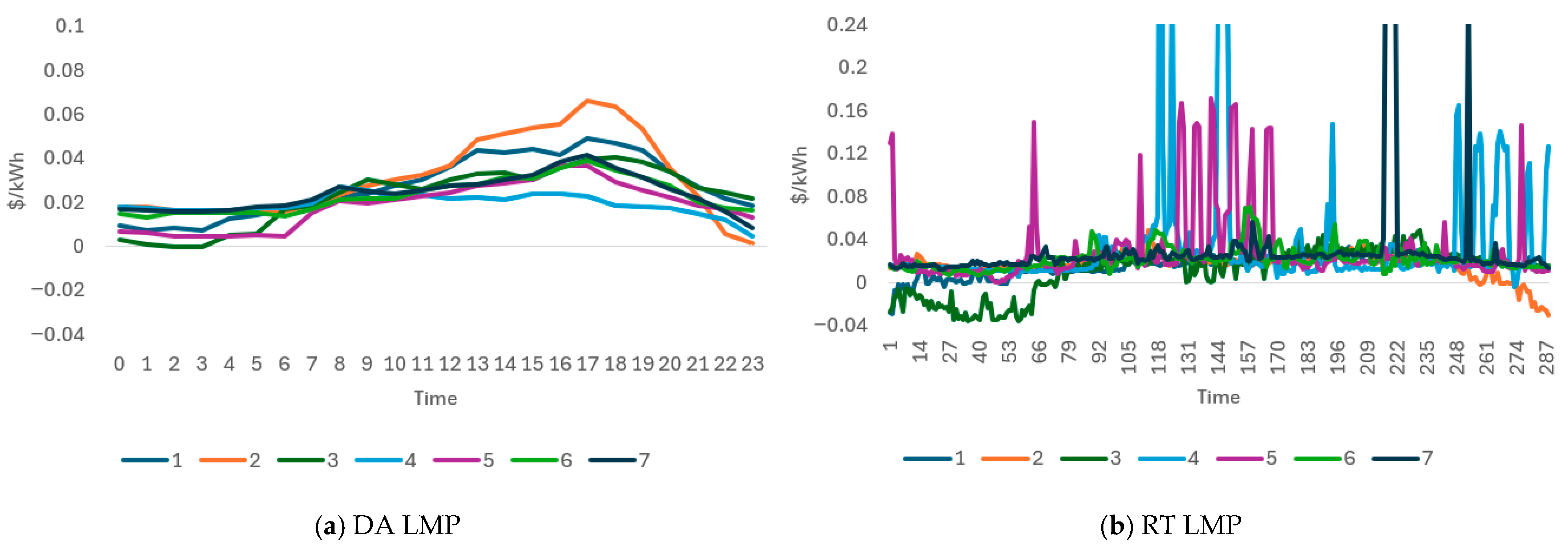
The two-stage VPP optimization was performed for 7 days, using consistent data across all modules. The period from 4 June to 10 June 2024, corresponds to Day 1 through Day 7, respectively. In the DA stage, charging sessions identified by the BFT were rescheduled to minimize expected power procurement costs based on hourly LMPs from the 2024 Southwest Power Pool (SPP) DA market in Figure 4a. In the RT stage, a 5 min interval problem was repeatedly solved to compensate for wind generation deviations and to respond dynamically to 5 min LMPs from the 2024 SPP RT market in Figure 4b. At each control step, only the first control action was implemented, and the optimization horizon was advanced in a receding horizon fashion to emulate RT operation.

Two comparative scenarios were simulated under identical meteorological and market conditions: the baseline scenario, which represents immediate charging without optimization, and the two-stage scenario, which integrates DA scheduling and RT optimization. EVs are charged at the day-ahead LMP during the day ahead scheduling stage, reflecting the settlement applied to scheduled charging. In the real-time stage, both charging and discharging actions use the real-time LMP signal. Furthermore, charging or discharging is allowed only when the expected net benefit, evaluated using the day ahead price, the real-time price, and the degradation cost is positive. Evaluation metrics included forecasting accuracy, behavioral indicators such as EV availability ratio, parking duration, and flexibility range, and operational outcomes including total cost, imbalance penalty, and flexibility utilization. This experimental setup establishes a reproducible, data-driven environment linking renewable forecasting, EV behavioral modeling, and market-based VPP optimization.

3.2. EV Behavioral Dynamics and Flexibility Traces

The daily mobility and charging patterns generated by the AB-TCC model were analyzed to evaluate their consistency with empirically observed travel behaviors from NHTS. Temporal distributions of departures and arrivals and dwell durations for each location were compared with those derived from the NHTS dataset to evaluate the behavioral consistency of the AB-TCC model.

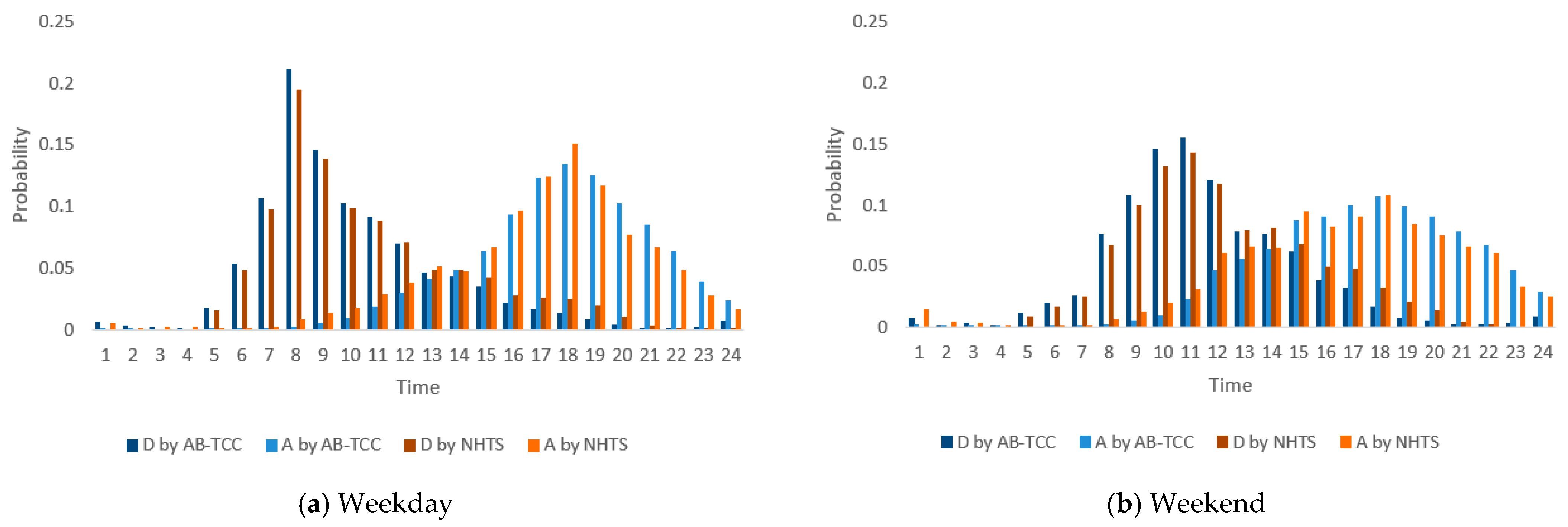
As shown in Figure 5, the departure and arrival time distributions generated by the AB-TCC model closely align with those observed in the NHTS dataset for both weekday and weekend.

Across four cases, the comparison between the AB-TCC model and NHTS data indicates a consistently high level of distributional agreement. The similarity metrics summarized in

Table 2. Distribution similarity metrics between AB-TCC and NHTS for weekday and weekend departure–arrival pairs.

Pair	MAE	RMSE	TVD (0–1)	Hellinger (0–1)	JS Distance (0–1)	Pearson r
Weekday-Departure	0.005	0.007	0.062	0.107	0.118	0.995
Weekday-Arrival	0.007	0.010	0.087	0.106	0.122	0.977
Weekend-Departure	0.006	0.008	0.078	0.132	0.142	0.987
Weekend-Arrival	0.007	0.009	0.084	0.096	0.114	0.978

show that the model closely matches empirical travel patterns across both weekdays and weekends. For weekday trips, both the departure and arrival distributions showed small average errors and low total variation distance, suggesting that the AB-TCC accurately reproduces the timing and shape of empirical commuting patterns. The Hellinger and Jensen-Shannon (JS) distances remained below 0.15, confirming strong similarity in overall probability structures, while the high Pearson correlations indicate nearly identical temporal dynamics between the simulated and observed distributions. For weekend trips, the departure and arrival distributions also exhibited a close correspondence to NHTS patterns. Although slightly larger Hellinger and JS distances for departure imply a broader temporal spread, the overall correlation remained high, showing that the AB-TCC effectively captures weekend behavioral variability as well. Overall, these results confirm that the AB-TCC model reproduces the empirical departure and arrival distributions from the NHTS dataset with high fidelity across both weekdays and weekends.

As shown in Figure 6, the AB-TCC model reproduces the location-specific dwell time patterns observed in the NHTS data for both weekdays and weekends. The simulated dwell durations across activity locations closely follow the empirical trends, demonstrating that the model captures the balance between travel and stay periods throughout the day.

The quantitative evaluation in

Table 3. Distribution similarity metrics between AB-TCC and NHTS for weekday and weekend dwell-time pairs.

Pair	MAE	RMSE	TVD (0–1)	Hellinger (0–1)	JS Distance (0–1)	Pearson r
Weekday-Dwell time	29.3	65.4	0.043	0.029	0.007	0.997
Weekend-Dwell time	44.4	106.5	0.046	0.032	0.009	0.996

shows small errors and RMSE and low divergence measures for both weekdays and weekends. For weekday trips, the AB-TCC showed a small average and RMSE along with low divergence measures, indicating that the AB-TCC closely reproduces the overall empirical dwell time pattern observed in the NHTS data. The high correlation confirms that the simulated dwell times capture the relative variation across destinations. However, the dwell time at home destination, representing TO = 10, appeared slightly shorter in the AB-TCC results than in the NHTS data, since agents incorporate charging behavior while traveling, which extends the overall travel time and consequently reduces the remaining time spent at home. The weekend results also exhibited a close correspondence. Overall, the AB-TCC model reproduces the empirical dwell time distributions with high fidelity while capturing realistic behavioral adjustments associated with EV charging.

As illustrated in Figure 7, the AB-TCC model endogenously generates time-dependent charging probabilities across different activity locations based on each agent’s SOC evolution and individual preferred SOC threshold. Charging is initiated when an agent’s SOC falls below this personalized threshold and continues during the available dwell time, subject to the rated charging power at each site. The resulting aggregated patterns align with typical U.S. charging behavior, showing that most charging events occur at home during evening and nighttime hours, while a smaller portion appears at workplaces and other public destinations during daytime.

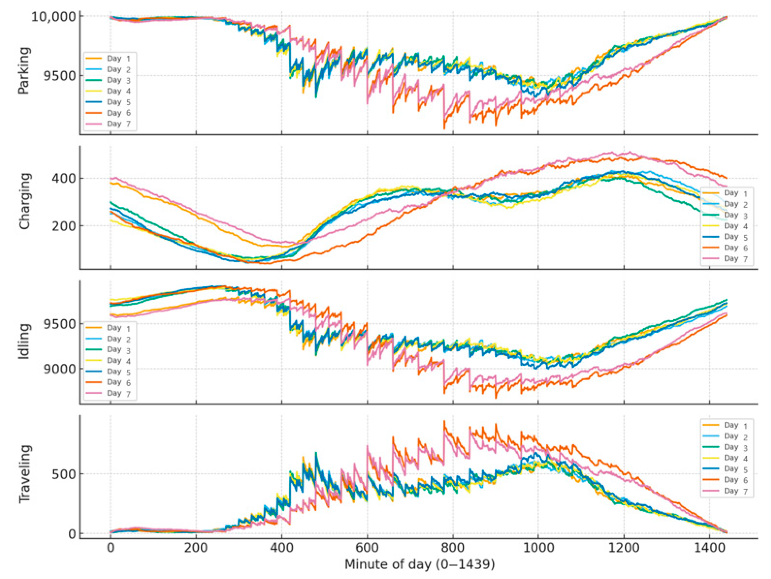
The temporal distribution of four EV states, such as Parking, Charging, Idling, and Traveling, at a one-minute resolution for each day of the simulation period is shown in Figure 8. These distributions were derived from the BFT, which records each EV’s transition between operational modes. Each line represents the number of EVs in a given state at a specific time of day, allowing for the direct observation of behavioral dynamics. The results show that most EVs remain parked or idle during nighttime hours, while traveling activity peaks during morning and evening commute periods. Charging events primarily occur in the late afternoon and evening, reflecting typical residential arrival patterns.

3.3. Wind Power Forecasting Results

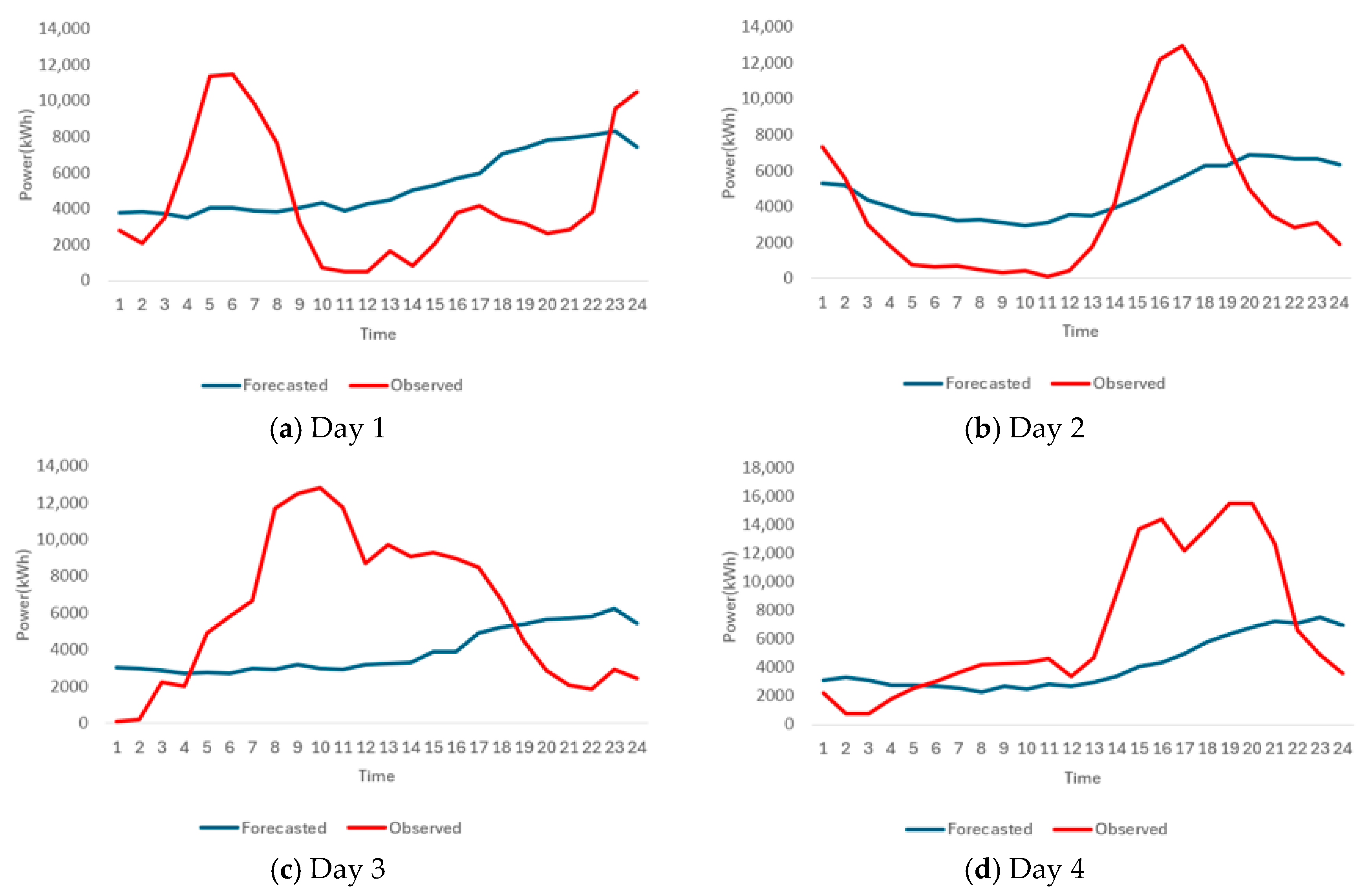
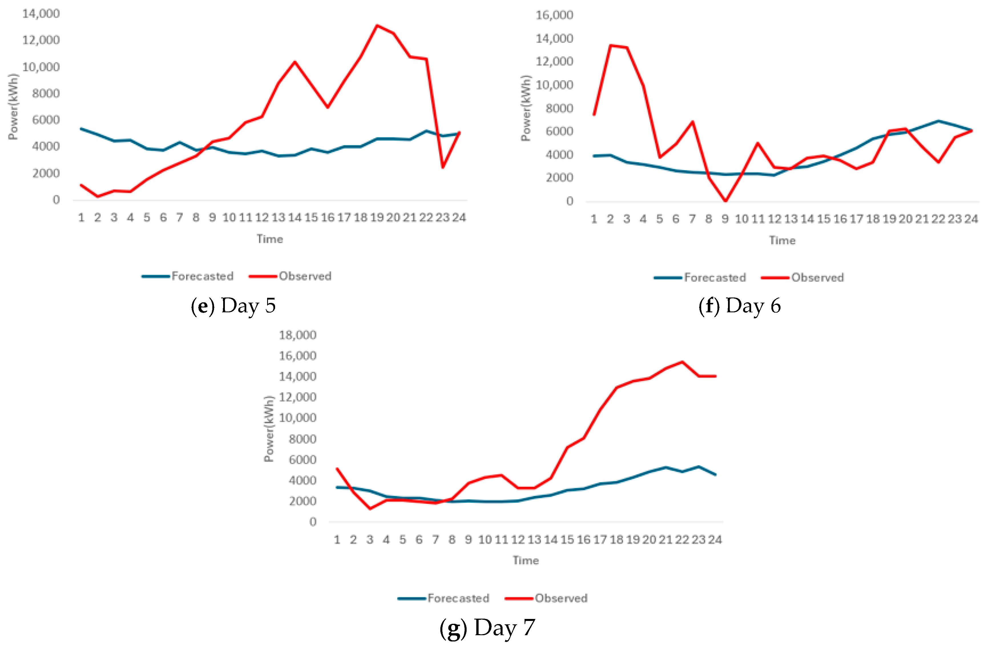
As shown in Figure 9, the predicted curves captured the main diurnal variations and ramping behavior, although slight underestimations and phase shifts appeared during high-output intervals. The corresponding performance metrics summarized in

Table 4. Comparison of total costs and imbalance penalties between baseline and optimized operation.

Day	MAE (kW)	NMAE (%)
1	3473.67	21.7
2	3012.62	18.8
3	4325.56	27.1
4	3689.75	23.1
5	3811.55	23.9
6	2316.14	14.5
7	4075.05	25.5

indicate that the forecasting model achieved stable accuracy, with low NMAE values across the evaluated days.

3.4. Two-Stage Scheduling Plan and Strategy of the VPP Operator

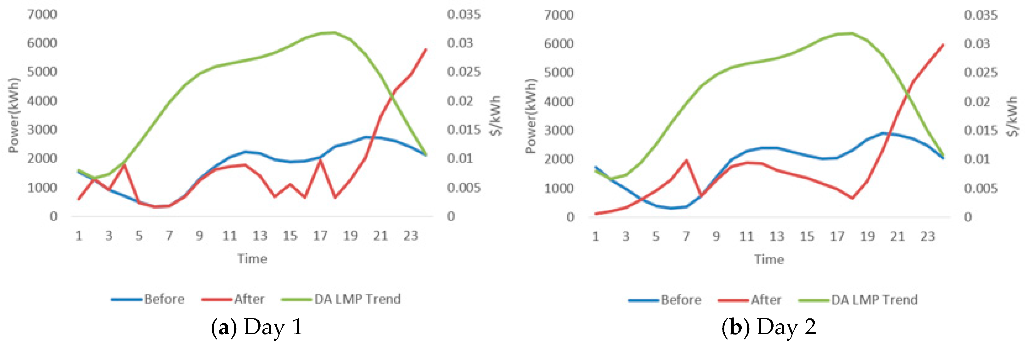
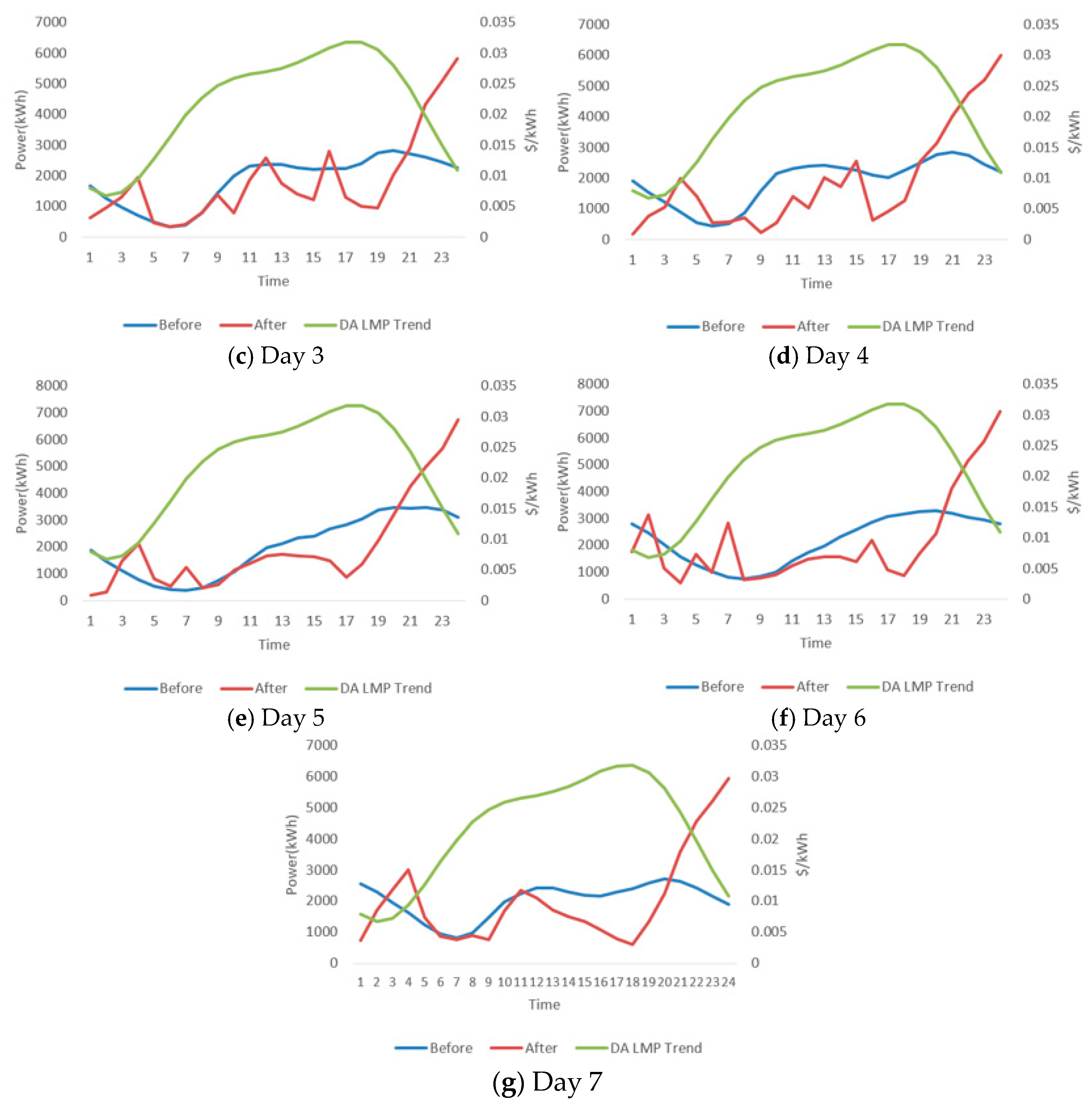
The hourly charging demand profile before and after applying the proposed two-stage optimization framework, is shown alongside the corresponding DA LMP trend in Figure 10. The blue line shows a relatively general EV charging pattern, whereas the red line shifts charging activities toward periods with a lower DA LMP trend, which is the green line.

Table 5. DA charging cost comparison between the baseline case and the proposed model.

Day	Charging Demands (kWh)	Baseline Cost ($)	Cost Saving ($)	DA Optimization Cost ($)	Cost Reduction (%)
1	41,445.9	1307.3	186.7	1120.6	14.3
2	43,616.8	1549.1	403.1	1146.0	26.0
3	44,083.1	1216.0	108.2	1107.8	8.9
4	45,263.2	881.5	136.7	744.8	15.5
5	48,067.5	1072.9	141.0	931.9	13.1
6	52,282.8	1293.9	160.6	1133.3	12.4
7	48,731.5	1230.6	185.5	1045.1	15.1

summarizes the DA charging costs under the baseline case with no coordinated control and under the proposed two-stage optimization framework. The results show that the optimized scheduling strategy for DA reduces daily charging expenditures, yielding cost savings between 8.9% to 26.0% across the 7 simulated days. Also, the result proves the effectiveness in reshaping the charging demand schedule without compromising EV operational feasibility.

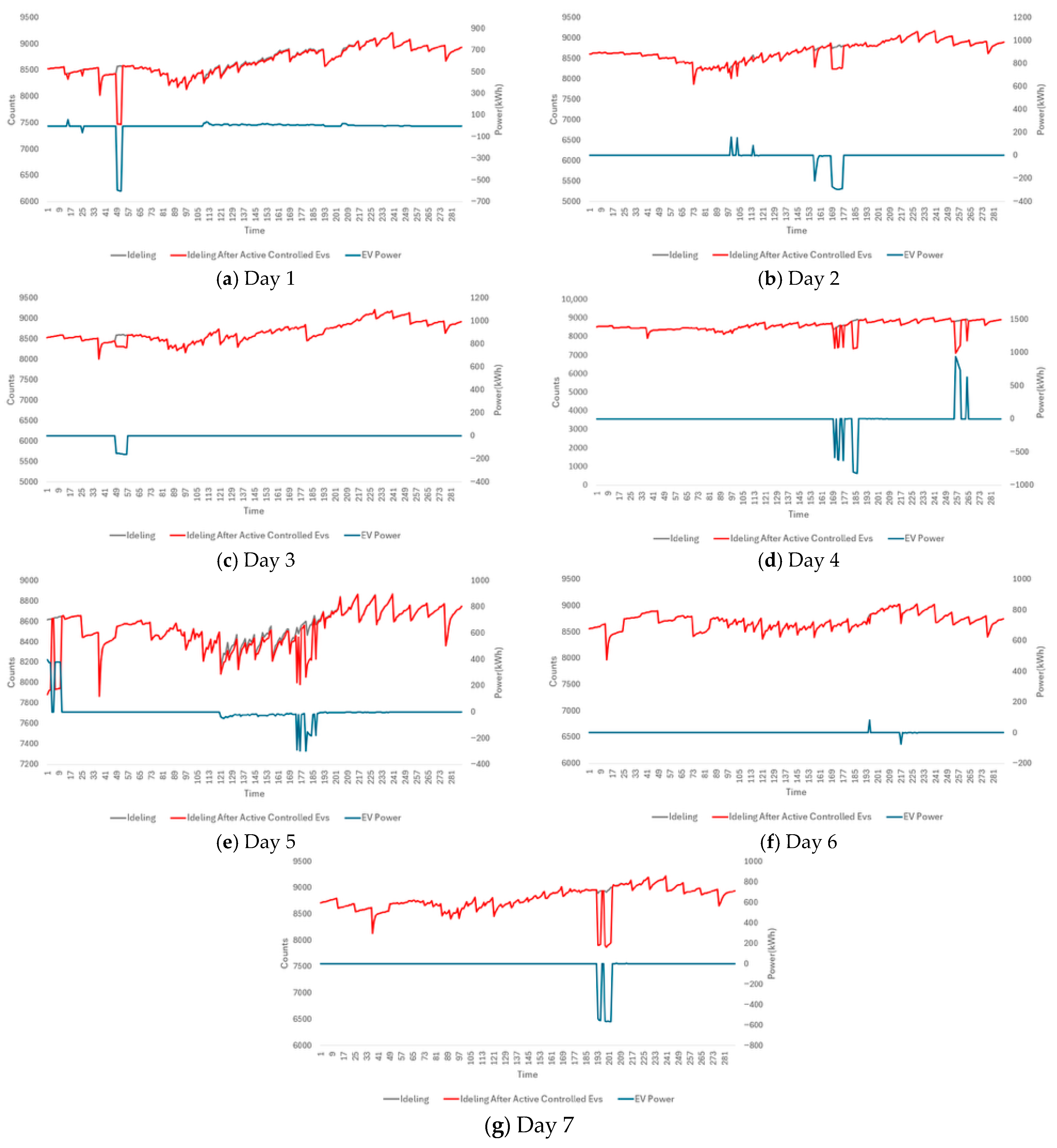
The RT optimization strategy is to control EV charging and discharging to minimize imbalance penalties by maintaining WT forecast deviations within the upper and lower 10% bounds. The results in

Table 6. Daily economic performance of RT optimization by controlling EVs.

Day	Baseline Net Revenue ($)	Net Revenue by Controlling EVs ($)	RT Optimization Net Revenue ($)	Battery Degradation Cost ($)	Discharging Power (kWh)	Charging Power (kWh)
1	651.34	13.46	664.80	8.45	1224.20	2450.03
2	−393.96	88.02	−305.94	7.22	445.81	2694.33
3	−414.70	40.22	−374.48	2.89	11.37	1243.16
4	277.08	492.98	770.06	22.49	4077.79	5702.30
5	165.96	104.05	270.01	14.50	3074.59	3229.51
6	38.08	3.57	41.65	0.38	83.41	81.79
7	2095.95	56.23	2152.18	10.40	54.16	4468.34

show that on days 2 and 3, WT forecast errors led to additional imbalance costs. However, from day 4 to day 7 and day 1, the imbalance adjustment turned into net benefits due to favorable differences between DA and RT market prices. Consequently, during days 4 to 7 and day 1, the optimization reduced WT forecast deviations while steering EV flexibility to maximize these market-driven benefits.

Table 6 reports how EV flexibility modifies daily net revenues by mitigating wind power forecast deviations and participating in RT market transactions. For all days, controlling EVs yielded substantial positive net revenue compared with the baseline, indicating effective compensation of penalties. Specifically, on day 2, the baseline deviation resulted in a $393.96 loss, but a net benefit of $88.02 was converted by controlling EVs. The daily charging and discharging volumes of the aggregated EV resource do not perfectly match because the economic conditions considered in the model, which include the difference between real-time and day ahead prices and battery degradation costs, interact with wind forecast errors in ways that vary across time. Because EVs make myopic decisions without access to future information, the optimal choice at a given time can lead to periods in which charging is selected repeatedly or, conversely, periods in which discharging is preferred. On day 5 and day 6, the constraints related to wind forecast deviations and the economic conditions tended to act in a more balanced manner, which produced relatively small differences between the total charging and discharging volumes. In contrast, on day 1, day 2, day 3, day 4, and day 7, the constraints that favored either charging or discharging became dominant during specific periods, leading to more pronounced directional behavior. Despite these imbalances, the resulting daily energy gap at the individual EV level remained very small. The average ranged from approximately −3.5 kW/h to +1.25 kW/h, which is negligible relative to typical daily driving energy consumption.

The model evaluates the economic viability of charging or discharging at each time step by combining the real-time price signal, the spread relative to the day ahead price, and the degradation cost associated with cycling in Figure 11. At the same time, deviations between forecasted and observed wind generation determine whether the power system requires charging or discharging in that moment. By tracking controllable EVs at 5 min intervals, the identified EVs are dispatched for real-time discharging and charging, and the remaining idle fleet is updated across day 1 to day 7 in Figure 12. This process enables the system to quantify the net power injection or withdrawal resulting from EV participation, as shown by the aggregated discharging and charging power profile.

3.5. Discussion

An important aspect of real-time EV dispatch is the balance between short-term revenue gains and battery degradation. In this study, we incorporated a degradation cost of 0.0023 $/kWh to monetize cycle-related battery wear, and the optimization permits charging or discharging when the expected profit exceeds this cost. This ensures that dispatch actions generate a positive net value while preventing excessive cycling that could undermine long-term battery health. Because the degradation cost reflects an amortized estimate of lifetime value loss, the resulting strategy remains economically sustainable even under extended operation.

For 7 days, the proposed two-stage scheduling model consistently outperformed the baseline strategy. The economic results indicate that the proposed model yielded approximately $145–600 of additional daily revenue, corresponding to a 5–32% improvement over the baseline in

Table 7. Total daily VPP economic performance relative to the baseline.

Day	Baseline Revenue ($)	DA Cost Saving ($)	RT Net Revenue ($)	Total Daily Benefit ($)	Proposed Model Revenue ($)
1	3122.44	186.67	5.01	191.68	3314.12
2	1747.38	403.04	80.80	483.84	2231.22
3	758.37	108.26	37.34	145.60	903.97
4	1244.79	136.72	470.49	607.21	1852.00
5	926.66	140.93	89.55	230.48	1157.14
6	1021.07	160.55	3.19	163.74	1184.81
7	2752.02	185.46	45.80	231.26	2983.28

. This performance improvement stems from effective DA scheduling that captures favorable price differentials, and from RT adjustments that reduce imbalance costs and secure short-term arbitrage opportunities. Combining behaviorally informed EV availability with a receding horizon RT optimization framework leads to robust and economically significant enhancements in VPP operations under a realistic energy market.

The results demonstrate that the proposed framework yields positive VPP operating revenues across a wide range of situations that combine different WT generation profiles with DA and RT LMP conditions. The VPP operator has partial visibility into system-level information, especially in the RT market where LMPs are published only five minutes ahead. Such limited foresight prevents the operator from fully exploiting EV flexibility. Moreover, to avoid interfering with the drivers’ travel behavior, the model enforces energy neutrality by requiring that each EV uses equal amounts of charging and discharging within a parking session. While this constraint helps preserve behavioral feasibility, the controller cannot always reduce wind forecast deviations to within the +10% band. In economically favorable intervals, the model accepts deviation penalties to increase overall revenue, resulting in several instances where deviations remain unmitigated. These patterns underscore the practical challenges arising from incomplete system information and suggest that enhanced information sharing with the system operator could further improve performance.

A key enabler of the proposed framework is the ability to estimate detailed EV states using the AB-TCC model, which makes the real-world EVs’ travelling and charging patterns. Access to individualized information such as parking duration, charging windows, idle time, and SOC proves essential for determining when EVs can be reliably dispatched as flexibility resources. The results illustrate that leveraging the EVs’ state estimates allows the VPP to utilize EV capacity without disrupting the EV drivers’ mobility needs. At the same time, incorporating battery degradation costs ensures that EV deployment remains economically neutral for participants, which is important for motivating EV driver participation.

This study integrates diverse datasets to construct a behaviorally and technically realistic simulation environment. The model uses region specific inputs for wind power generation, local meteorological conditions, and LMPs. Other inputs rely on information that originates from different geographical contexts such as household trip patterns in the United States, vehicle registration data from Colorado, and EV charging behavior observed in Korea. These differences in source materials can create inconsistencies in behavioral assumptions and in the resulting aggregated model outcomes.

Therefore, we recognize this limitation and emphasize that the present analysis serves as a modeling based demonstration of the proposed methodology rather than a study intended for direct policy application within a specific region. Future research should apply the same framework to datasets that share a single spatial context. Such an effort would allow for a more rigorous assessment of the robustness and contextual relevance of the proposed model when it is evaluated under realistic deployment conditions.

4. Conclusions

This study proposed an integrated, data-driven framework that combines wind generation forecasting, agent-based EV behavioral modeling, and two-stage VPP optimization. The framework links the physical dynamics of renewable variability with the behavioral flexibility of EV users and market-based coordination mechanisms. The study advances methodological understanding by employing agent-based modeling to reconstruct minute-level EV mobility and charging patterns and by formalizing these behavioral dynamics into a Behavioral Flexibility Trace that represents the flexibility available for VPP operations. To evaluate its performance, a 7-day experimental implementation was conducted using several data sources, each serving a distinct role in the framework. ERA5 meteorological data were used to generate wind power forecasts. SPP day ahead and real-time market prices provided the price signals required for the two-stage VPP optimization. The mobility patterns of the 10,000 simulated EV agents were produced through the AB-TCC model, which was calibrated using NHTS travel statistics, Colorado EV fleet composition data, and survey based behavioral characteristics collected from South Korean EV drivers. This combination of datasets allowed the case study to capture both the physical variability of renewable generation and the behavioral diversity of EV users. To evaluate its performance, a 7-day experimental implementation was conducted using ERA5 meteorological data, SPP day-ahead and real-time market prices, and mobility patterns derived from 10,000 simulated EV agents calibrated with NHTS statistics, Colorado vehicle composition, and Korean driver survey data. The results demonstrate that the proposed two-stage VPP operation yielded significant economic and operational benefits compared with the baseline scenario. Over the 7-day test horizon, total revenue increased by 15%, driven by cost-efficient charging rescheduling in the day-ahead stage and real-time charging and discharging that adjust deviation outcomes to reduce losses or augment gains. Aggregated EV flexibility improved real-time financial performance by mitigating the cost impacts of wind forecast deviations, effectively functioning as distributed virtual storage. Temporal analysis revealed that the coordinated scheduling aligned charging with low-price, high-wind periods and discharging with evening price peaks, improving load factor and renewable utilization. These findings highlight the dual value of EVs as mobile energy consumers and as distributed flexibility resources when their behavioral characteristics are realistically modeled. By incorporating empirically derived mobility and charging preferences, the framework ensures that optimization results are both economically viable and behaviorally feasible. From a market perspective, the approach demonstrates how short-term, high-resolution coordination between EV fleets and renewable generation can stabilize system operations and reduce settlement costs, even without explicit network-level control. Policy wise, the results suggest that expanding EV participation in real-time markets, supported by data-driven forecasting and aggregator level optimization, can enhance both market efficiency and renewable integration. As electricity markets adopt shorter settlement intervals and EV adoption accelerates, behavior-aware coordination mechanisms such as the one proposed here will become increasingly vital for achieving reliable, low-carbon power systems. Future research should extend this framework to multi region or multi resource settings and examine the interactions between behavioral uncertainty, network constraints, and market design.

References

1. Gao, H.; Wang, Y.; Zhang, H.; Wang, Y. Review of virtual power plant operations: Resource coordination and multidimensional interaction. Appl. Energy 2024, 357, 122284. [Google Scholar] [CrossRef]
2. Feng, J.; Ran, L.; Wang, Z.; Zhang, M. Optimal energy scheduling of virtual power plant integrating electric vehicles and energy storage systems under uncertainty. Energy 2024, 309, 132988. [Google Scholar] [CrossRef]
3. Kumar, P.; Kumar, N.M.; Saha, T.K.; Shukla, A.K.; Sharma, P.; Singh, B. A comprehensive review of vehicle-to-grid integration in electric vehicles: Powering the future. Energy Rep. 2024, 10, 100517. [Google Scholar] [CrossRef]
4. Gerritsma, M.K.; AlSkaif, T.A.; Fidder, H.A.; van Sark, W.G.J.H.M. Flexibility of Electric Vehicle Demand: Analysis of Measured Charging Data and Simulation for the Future. World Electr. Veh. J. 2019, 10, 14. [Google Scholar] [CrossRef]
5. Niu, J.; Li, X.; Tian, Z.; Yang, H. Uncertainty analysis of the electric vehicle potential for a household to enhance robustness in decision on the EV/V2H technologies. Appl. Energy 2024, 365, 123294. [Google Scholar] [CrossRef]
6. Yi, Z.; Xu, Y.; Gu, W.; Yang, L.; Sun, H. Multi-time-scale scheduling strategy for virtual power plants considering uncertainty. IEEE Trans. Sustain. Energy 2020, 11, 4208–4224. [Google Scholar] [CrossRef]
7. Vahedipour-Dahraie, M.; Najafi, H.R.; Anvari-Moghaddam, A.; Guerrero, J.M. Risk-averse scheduling of virtual power plants in energy and reserve markets considering demand response programs. IEEE Trans. Smart Grid 2020, 11, 2964–2976. [Google Scholar]
8. Abbasi, M.H.; Fotuhi-Firuzabad, M.; Rastegar, M. Coordinated operation of electric vehicle charging and wind power generation as a virtual power plant. Appl. Energy 2019, 256, 113961. [Google Scholar]
9. Ren, L.; Wang, Q.; Chen, Y.; Wang, Y.; Zhou, X.; Li, J. Multi-objective dispatching optimization of virtual power plants in vehicle-to-grid mode. Front. Energy Res. 2023, 11, 1178273. [Google Scholar]
10. Fang, F.; Hu, Y.; Li, J.; Xu, Y.; Liu, J. Data-driven stochastic robust optimization for virtual power plant operation under renewable and market uncertainty. IEEE Trans. Power Syst. 2022, 37, 4965–4976. [Google Scholar] [CrossRef]
11. Geng, S.; Zhang, T.; Li, K.; Liu, P. Optimal allocation model of virtual power plant capacity considering electric vehicles. Math. Probl. Eng. 2021, 2021, 6658437. [Google Scholar] [CrossRef]
12. Sun, W.; Li, Q.; Wang, C.; Liu, X.; Zhang, P. Electric power dispatching of virtual power plant with electric vehicles. J. Phys. Conf. Ser. 2022, 2275, 012026. [Google Scholar] [CrossRef]
13. Gao, Y.; Chen, R.; Liu, H.; Zhang, Z. The optimal energy management of virtual power plants with electric vehicles based on information gap decision theory. Processes 2025, 13, 157. [Google Scholar]
14. González-Romera, E.; Amarís Duarte, J.; Romero-Cadaval, E. A genetic algorithm for residential virtual power plants: Optimal day-ahead scheduling of storage and electric vehicles. Electronics 2023, 12, 3717. [Google Scholar] [CrossRef]
15. U.S. Department of Transportation, Federal Highway Administration. National Household Travel Survey. 2022. Available online: http://nhts.ornl.gov (accessed on 17 March 2025).
16. Power Systems Economics Laboratory, Gwangju Institute of Science and Technology. EV Driving and Charging Data Repository for the Converged Charging Station R&D Project. 2024. Available online: http://psel.gist.ac.kr/prog/bbsArticle/BBSMSTR_000000011963/view.do?nttId=B000000069959Np1yY3w&mno=59118 (accessed on 15 May 2025).
17. Hersbach, H.; Bell, B.; Berrisford, P.; Biavati, G.; Horányi, A.; Muñoz Sabater, J.; Nicolas, J.; Peubey, C.; Radu, R.; Rozum, I.; et al. ERA5 Hourly Data on Single Levels from 1940 to Present. Copernicus Climate Change Service (C3S) Climate Data Store (CDS). Available online: https://cds.climate.copernicus.eu (accessed on 23 June 2025).
18. Preis, V.; Biedenbach, F. Assessing the incorporation of battery degradation in vehicle-to-grid optimization models. Energy Inf. 2023, 6, 33. [Google Scholar] [CrossRef]
19. Atlas EV Hub. State EV Registration Data. Available online: http://www.atlasevhub.com/market-data/state-ev-registration-data/ (accessed on 12 May 2025).
20. U.S. Geological Survey (USGS); Lawrence Berkeley National Laboratory (LBNL); American Clean Power Association (ACP). U.S. Wind Turbine Database (USWTDB). Available online: http://eerscmap.usgs.gov/uswtdb/ (accessed on 30 June 2025).
Figure 1. Overall architecture of the proposed framework for VPP operation.
Sustainability 17 11291 g001
Figure 2. Market-weighted composition of the simulated AB-TCC fleet.
Sustainability 17 11291 g002
Figure 3. Power curves of the turbines.
Sustainability 17 11291 g003
Figure 4. Market prices.
Sustainability 17 11291 g004
Figure 5. Departure and arrival distributions (AB-TCC vs. NHTS).
Sustainability 17 11291 g005
Figure 6. Dwell time by location (AB-TCC vs. NHTS).
Sustainability 17 11291 g006
Figure 7. Charging probability by location.
Sustainability 17 11291 g007
Figure 8. EV state counts by day.
Sustainability 17 11291 g008
Figure 9. Actual and forecasted WT power.
Sustainability 17 11291 g009aSustainability 17 11291 g009b
Figure 10. Optimized EV charging load shifting relative to DA LMP trend.
Sustainability 17 11291 g010aSustainability 17 11291 g010b
Figure 11. Coordinated EV flexibility response to WT deviations under RT LMP.
Sustainability 17 11291 g011
Figure 12. EV state transitions and aggregated participation in charging and discharging operations.
Sustainability 17 11291 g012