Article

Do Carbon Emissions Hurt? Novel Insights of Financial Development and Economic Growth Nexus in China

School of Finance, Southwestern University of Finance and Economics, Chengdu 611130, China
*
Author to whom correspondence should be addressed.
Sustainability 2025, 17(24), 11249; https://doi.org/10.3390/su172411249
Submission received: 6 October 2025 / Revised: 3 December 2025 / Accepted: 10 December 2025 / Published: 16 December 2025
(This article belongs to the Section Economic and Business Aspects of Sustainability)

Abstract

This paper examines whether financial development affects economic growth across different levels of carbon emissions in 30 Chinese provinces from 1990 to 2022. We employ a novel partially linear functional-coefficient model with latent factor structure. This approach relaxes the traditional assumptions of linearity and cross-sectional independence, allowing us to capture more flexible growth patterns. Our empirical findings reveal three key insights: (i) the positive effect of financial development on economic growth follows a nonlinear pattern—it initially strengthens as carbon emissions increase but declines rapidly after emissions reach a threshold; (ii) innovation and openness show limited impacts on economic growth; (iii) regional variations exist based on resource endowment. These findings offer important policy implications. Promoting green financial products could extend the beneficial range of carbon emissions for economic growth. Optimizing innovation structures and supervising foreign enterprises may help unlock growth potential while preventing pollution transfer. Regional strategies would benefit from accounting for resource disparities.

1. Introduction

Financial development has been recognized as a pivotal factor in economic performance since its significant impact on economic growth was confirmed [1]. Greater financial resources enhance capital allocation efficiency, encourage investment, and reduce information costs [2,3,4]. However, as global climate change intensifies, economic and financial activities are increasingly influenced by climate and energy factors [5], making economic dynamics more intricate.
Scholars have begun investigating the complex economic implications of financial development in relation to climate and energy [6,7,8,9,10,11]. Carbon emissions have emerged as a foremost environmental concern due to global warming [12,13,14,15,16,17]. For China, achieving peak carbon dioxide emissions (peak carbon dioxide emissions refers to a point in time when carbon dioxide emissions stop growing and reach their peak, after which they gradually decline) and carbon neutrality are critical strategic goals [18]. (Carbon neutrality refers to achieving net-zero greenhouse gas emissions from human activities by maximizing emission reductions through energy conservation and emission reduction measures, combined with anthropogenic atmospheric greenhouse gas removal (negative carbon emissions). Negative emissions offset the remaining emissions that cannot be avoided by existing energy conservation and emission reduction measures, thereby achieving net-zero carbon footprint from human activities and a relatively dynamic balance in the atmospheric carbon cycle.) On 22 September 2020, China announced at the 75th United Nations General Assembly its commitment to achieve peak emissions before 2030 and carbon neutrality before 2060. However, as Figure 1 illustrates, the relationship between carbon emissions and financial development is nonlinear, with financial development appearing constrained when emissions are either very low or very high. This pattern raises questions about the underlying dynamics among carbon emissions, financial development, and economic growth.
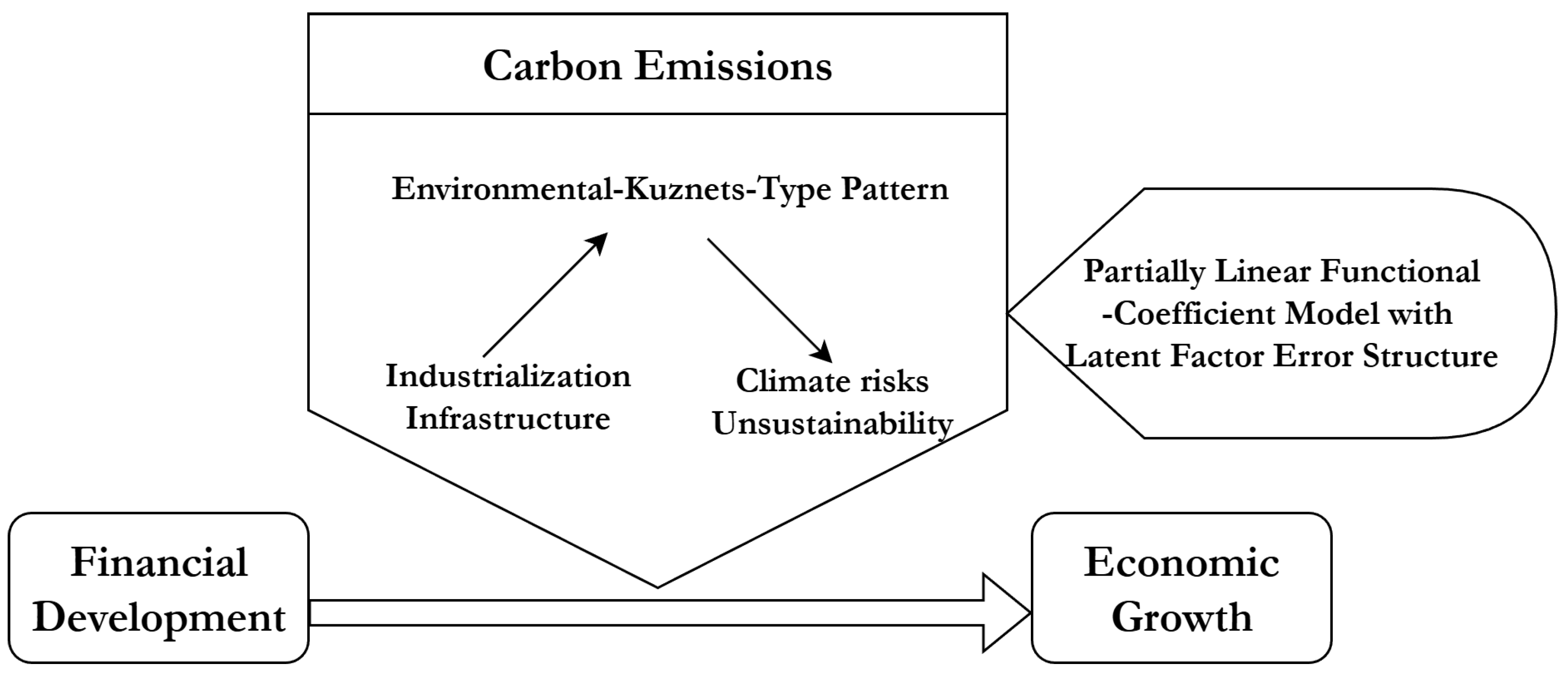
The literature suggests carbon emissions shape financial development’s impact on growth in a nonlinear, environmental-Kuznets-type pattern. At low to moderate emission levels, higher emissions often indicate finance-funded industrialization that reinforces finance’s positive impact on GDP per capita [19,20,21]. Beyond a threshold, emissions reflect an unsustainable carbon-intensive model where finance deepens exposure to fossil fuels and climate risks, weakening or reversing the growth payoff [22].
To investigate the above dynamics, existing studies often employ linear models or nonlinear models such as regime switching [8,23]. However, several issues remain unaddressed. First, these models rarely address endogeneity arising from the bidirectional causality between financial development and economic growth. Second, provincial panel data covering nearly all Chinese provinces cannot be considered a random sample, suggesting potential cross-sectional dependence. Third, regime switching models assume a finite number of regimes, which may not reflect reality. Drawing inspiration from recent methodological advances [24], we propose a partially linear functional-coefficient model with latent factor error structure (Figure 2). This model accommodates endogeneity by allowing explanatory variables, smooth variables, and error terms to share a similar factor structure. The factor error structure captures cross-sectional dependence [25], while the varying coefficient specification enables coefficients to be nonlinear functions of certain variables. We also propose a test statistic for model selection between our approach and regime switching models.
Our methodology offers three key contributions. First, our functional-coefficient model allows for flexible, smooth nonlinear effects rather than discrete structural breaks through limited thresholds. This better reflects reality, as environmental issues arising from long-term accumulations necessitate gradual economic responses.
Second, we account for cross-sectional dependence through a semi-parametric model with common factor structure. While previous studies assume independence among economies, regional economic activities are actually influenced by common factors. This is particularly relevant for Chinese provincial data, which cannot be treated as independent random samples. Accounting for cross-sectional dependence substantially improves accuracy.
Third, we explore regional heterogeneity beyond cardinal directions. Given China’s dispersed distribution of energy resources, we categorize samples by resource abundance to investigate interactive patterns among carbon emissions, financial development, and economic growth. This approach provides more accurate mechanistic understanding and policy recommendations.
The remainder of the paper is structured as follows. Section 2 provides the literature review. The econometric methodology of this study is outlined in Section 3. The data sources and empirical results analysis are presented in Section 4. Section 5 gives the conclusion and policy suggestion.

2. Literature Review

Financial development and various economic factors have long been recognized as drivers of economic growth, though their effects remain debated. Following the foundational work on financial deepening [26,27], numerous studies confirm that financial development promotes growth by improving resource allocation, enhancing corporate governance, and encouraging investment [1,2,4,28,29]. However, recent research challenges this simple positive relationship, revealing weakened links [30] and threshold effects beyond which financial development negatively impacts growth [31,32,33].
Beyond finance, technological innovation and trade openness are widely studied growth determinants. Theoretical and empirical work emphasizes innovation as a primary growth driver [34,35,36], though its benefits may diminish with low technology transfer rates [37,38]. Similarly, while openness can promote growth through technology transfers and comparative advantage [39], its effects vary by income level [40] and may be limited or even negative due to pollution transfer [38,41]. Overall, no consensus exists regarding these factors’ growth effects.
As environmental concerns intensify, research increasingly examines how carbon emissions affect economic growth [12,13,14,15,16,17]. Studies yield mixed findings: some show emissions significantly undermine growth [42], others find short-term negative but no long-term effects [43], while still others document positive impacts in both the short and long run [44]. Recent work reveals that carbon emissions and environmental factors interact with traditional growth determinants, modifying their marginal effects. Research employing threshold models [45] and panel smooth transition regression [8] demonstrates that carbon emissions attenuate the positive effects of financial development, innovation, and other growth factors.
Beyond these direct effects, carbon emissions play a central role in shaping how financial development translates into economic growth, and this moderating influence is inherently nonlinear. At early and intermediate stages of development, rising emissions often reflect industrialization, urbanization, infrastructure construction, and expansion of modern energy use. In this phase, financial development that accompanies higher emissions typically finances factories, transport networks, power plants, and housing—activities that raise productivity and income. Consequently, at low to moderate emission levels, carbon emissions can strengthen the positive effect of financial development on real GDP per capita, serving as a by-product of growth-enhancing structural transformation [19,20,21]. Beyond a certain threshold, however, additional emissions increasingly signal a carbon-intensive and environmentally unsustainable growth model. At high emission levels, particularly in resource-abundant economies, financial development may reinforce over-reliance on fossil fuels, heavy industry, and other high-carbon sectors, exposing the economy and financial system to transition risks—including stricter climate policies, carbon pricing, and global demand shifts away from fossil fuels—as well as physical risks from climate change and local environmental degradation. These risks lower productivity, weaken human capital, and increase the likelihood of stranded assets, thereby attenuating or even reversing the growth benefits of financial development [5,22].
A political economy perspective also helps explain the mechanisms underlying this redirection. Rising emissions reshape the institutional and regulatory environment in which finance and growth interact. As climate damages and mitigation commitments mount, governments and international organizations expand carbon pricing and regulatory interventions—such as domestic carbon taxes, emissions trading systems, and border instruments like the EU Carbon Border Adjustment Mechanism (CBAM)—that effectively tax carbon-intensive production and alter relative prices between “brown” and “green” activities [5,46]. These measures interact with international financial regulation and emerging green finance policies—including climate-related disclosure standards, green taxonomies, and prudential rules that differentiate capital requirements for high-carbon exposures—thereby shifting banks’ and capital markets’ incentives away from carbon-intensive sectors toward low-carbon technologies [47,48]. In coordinated regimes such as the EU, strong state-market relations enable public policy to use financial regulation and carbon pricing jointly to steer private capital, amplifying the redirection effect on financial development’s growth impact. Conversely, in weaker or more fragmented governance systems, lobbying by incumbent fossil fuel and heavy-industry interests can dilute or delay such policies, allowing financial deepening to continue channeling resources into high-emission activities and locking in carbon-intensive capital stock [49].
To empirically identify this nonlinear moderating role of carbon emissions, appropriate methodological considerations are essential. Most studies investigating nonlinear patterns in economic growth mechanisms rely on threshold models, which assume that nonlinearity is discontinuous with structural breaks [32,33,45,50]. Yet the impact of carbon emissions on the finance-growth relationship tends to be gradual rather than abrupt. Recent research applies a smooth transition function to threshold regimes, thereby extending the threshold model into a continuous framework [8]. Nevertheless, this approach still requires pre-setting a finite number of regimes, indicating limited capability to capture complex nonlinear dynamics. The partially linear functional-coefficient model treats the coefficient of renewable energy technology as a function of the income gap to capture more flexible nonlinear relationships among variables [51]. This approach, though more flexible, overlooks cross-sectional dependence among provinces in China, which typically exists for economies influenced by common factors such as national policies, technological spillovers, and macroeconomic shocks. In the existing literature on economic growth processes, consideration of cross-sectional dependence is largely limited to conducting panel cointegration tests aimed at demonstrating the robustness of long-run cointegration relationships among variables [45,52]. For specific nonlinear relationships, the incorporation of cross-sectional dependence in the estimation process remains unexplored.
We summarized the main related studies in Table 1. The existing literature reveals three critical gaps that motivate this study. First, while recent research recognizes that carbon emissions interact with financial development to influence economic growth, the empirical modeling of this interaction remains limited by restrictive parametric assumptions. Threshold models impose discrete structural breaks, and smooth transition regression models require pre-specification of regime numbers, neither of which adequately captures the gradual and continuous nature of carbon emissions’ moderating effect on the finance-growth relationship. Second, methodological approaches have largely neglected cross-sectional dependence in estimating nonlinear growth relationships, despite compelling evidence that economies—particularly those within integrated regions—are subject to common policy shocks, technological spillovers, and macroeconomic conditions that generate correlated outcomes. Third, although theoretical arguments suggest that carbon emissions may nonlinearly moderate financial development’s growth impact through both biophysical constraints and evolving regulatory frameworks, no empirical framework has systematically tested this inverted U-shaped relationship while accounting for both methodological concerns.
The theoretical framework developed in this chapter posits a nonlinear moderating effect of carbon emissions on the finance-growth relationship, driven by both biophysical and political-institutional thresholds. At relatively low emission levels, the marginal effect of financial development on growth tends to increase as emissions rise, because higher emissions capture the scale-up of productive, growth-enhancing activities and precede the most stringent stages of climate policy. After emissions pass a critical level, further increases not only intensify environmental and climate-related risks but also trigger more aggressive carbon pricing, green regulation, and trade measures such as CBAM, which reprice high-carbon assets, distort previous allocation patterns, and raise macro-financial vulnerabilities. Specifically, resource-abundant areas reach this critical threshold at lower emission levels than resource-moderate and resource-scarce areas due to earlier exposure to transition risks and carbon lock-in in fossil fuel-dependent economies. The relationship between financial development, carbon emissions, and economic growth thus resembles an inverted U-shape: finance supports growth more strongly as emissions rise up to a turning point, but beyond that point, the combination of environmental damage, tighter climate policy, and green financial regulation progressively erodes—and may eventually reverse—the growth benefits of financial development for real GDP per capita.
Drawing on the theoretical framework above, we propose a conceptual framework in which carbon emissions nonlinearly moderate the finance-growth relationship through two competing mechanisms. At low-to-moderate emission levels, rising emissions signal industrialization and structural transformation that stimulate green finance development, expanding financial intermediation opportunities and reinforcing finance’s positive growth effect. Beyond a critical threshold, however, elevated emissions reflect unsustainable carbon-intensive models that expose financial systems to transition risks, stranded assets, and climate-related uncertainties, thereby weakening or reversing the growth contribution of financial development.
This framework generates two testable hypotheses:
H1 (Inverted-U Pattern):
The marginal effect of financial development on economic growth follows an inverted-U pattern, initially increasing with carbon emissions but declining after reaching a threshold level.
H2 (Resource Heterogeneity):
The threshold occurs at lower emission levels in resource-abundant provinces compared to resource-moderate and resource-scarce regions.
To empirically test our hypotheses, this paper proposes a partially linear functional-coefficient model with cross-sectional dependence that investigates the flexible nonlinear relationship among carbon emissions, financial development, and economic growth. We model the coefficient of financial development as a smooth, non-parametric function of carbon emissions, allowing the data to reveal the shape of this moderating effect without imposing restrictive functional forms or pre-specified regimes. Other established growth determinants—trade openness, technological innovation, and total capital—are incorporated to form a latent factor error structure that explicitly accounts for cross-sectional dependence arising from common shocks and regional spillovers. Our methodology builds upon and extends recent advances in panel data estimation with interactive fixed effects [24], adapting them to a partially linear framework that enhances interpretability while preserving desirable asymptotic properties. This approach enables us to simultaneously capture the continuous nature of carbon emissions’ threshold effect and the interdependencies among economies, providing a more comprehensive characterization of how environmental factors reshape the finance-growth nexus.

3. Methodology

3.1. The Baseline Model

We build upon the classical endogenous growth literature, specifically the Cobb–Douglas extended production function “AK” model where aggregate output is a linear function of the aggregate capital stock: y = A K [53,54]. This production function has been widely accepted as a reduced form model for empirical testing in the long stream of economic growth and the financial development literature. Thus, we begin with the following Cobb–Douglas extended production function:
Y = A L β K α e ϵ
with
α + β = 1
where Y is the real GDP, A is the total factor productivity, K is the capital stock, L is the labor force, ϵ is the error term, and α and β are the output elasticities of labor and capital, respectively.
Referring to [8,55], we assume that technology evolves endogenously through innovation, financial development, and economic openness and have
Y = θ · F D σ × I N N γ × O P E N ω × L ϕ × K μ × e ϵ
with
σ + γ + ω + ϕ + μ = 1
where F D ,   I N N , and O P E N represent financial development, innovation, and economic openness, respectively.
Dividing Equation (2) by L:
Y L = θ F D L σ I N N L γ O P E N L ω K L μ e ε
Taking logarithms of Equation (3), we then construct the log-linear function:
y i t = β i + β 1 f d i t + β 2 i n n i t + β 3 o p e n i t + β 4 k i t + ε i t
where y ,   f d ,   i n n ,   o p e n , and k represent the logarithms of corresponding per capita variables, i = 1 ,   2 ,   ,   N denote the cross-section unit, and t = 1 ,   2 ,   ,   T are the indices for time.
To explore the heterogeneous effect of financial development regarding the carbon emission levels, we consider models with interactive term. We first consider the absolute carbon emission level:
y i t = β i + β 1 f d i t + γ f d i t × c a r b o n i t + β 2 i n n i t + β 3 o p e n i t + β 4 k i t + ε i t
where c a r b o n i t is the carbon emissions.
Then we consider the relative carbon emission level:
y i t = β i + β 1 f d i t + γ f d i t × c a r b o n g a p i t + β 2 i n n i t + β 3 o p e n i t + β 4 k i t + ε i t
where c a r b o n g a p i t = c a r b o n i t / m a x c a r b o n i t .
Alternatively, we consider the following equation:
y i t = β i + β 1 f d i t + γ f d i t × D i t + β 2 i n n i t + β 3 o p e n i t + β 4 k i t + ε i t
where the dummy variable D i t equals one when the carbon emissions is higher than the median, and zero otherwise.

3.2. The Semi-Parametric Model with Cross-Sectional Dependence

The models from (5) to (7) face misspecification issues due to the linear assumptions on the effect of financial development. Moreover, the estimations may be inconsistent since the possible cross-sectional dependence is ignored. In light of these, Ref. [24] proposed a non-parametric panel data model that accounts for cross-sectional dependence. However, this model assumes that all independent variables have functional coefficients, which is difficult to justify in practice. We extend it to a partially linear framework, where the coefficient of the core explanatory variable is a nonlinear function of carbon emissions, but the coefficients of the remaining explanatory variables remain constant. Using estimation and proof steps similar to those in [24], we can estimate the newly proposed model and demonstrate that the estimator possesses desirable asymptotic properties.
The extended model is as follows:
y i t = β 1 ( U i t ) · f d i t + β 2 · i n n i t + β 3 · o p e n i t + β 4 · k i t + γ 1 i f 1 t + e i t
where β 1 ( · ) is an unknown smooth function defined on R , which has a continuous second derivative, U i t is the smooth variable that represents carbon emissions here, f 1 t is a m 1 × 1 vector of observed common factors, which includes the intercept term, γ 1 i is the factor loading and e i t is the error term with multi-factor structure as below:
e i t = γ 2 i f 2 t + ε i t
where f 2 t is a m 2 × 1 vector of unobserved common factors, γ 2 i is the factor loading, and ε i t is the idiosyncratic error of y i t .
Denote X i t = ( f d i t , i n n i t , o p e n i t , k i t ) . We allow the unobserved common factor f 2 t be correlated with both the independent variable X i t and the smooth variable U i t :
Z i t = X i t U i t = Γ 1 i f 1 t + Γ 2 i f 2 t + v i t
where Γ 1 i is the m 1 × 5 factor loading of observed common factors, Γ 2 i is the m 2 × 5 factor loading of unobserved common factors, and v i t is the idiosyncratic error of Z i t . This structure implies that both explanatory and smoothing variables can be endogenous.
To clarify, this structure could address endogeneity arising from omitted variable bias (common factors) and simultaneous causality operating through common factors. For omitted variable bias, latent factors f 2 t could capture unobserved national-level policy shocks, macroeconomic conditions, and technological spillovers. For example, a national stimulus package in 2009 simultaneously boosted provincial GDP growth ( y i t ), expanded bank lending ( f d i t ), and increased industrial emissions ( c a r b o n i t ). Without controlling for this common shock, we would spuriously attribute the growth-finance correlation to financial development’s causal effect. The factor structure absorbs this f 2 t component. For simultaneous causality, the key mechanism here is that Equation (10) models financial development ( f d i t , part of X i t ) as being driven by the same latent factors f 2 t that appear in the growth equation’s error term. Consider the reverse causality problem: economic growth ( y i t ) may stimulate financial development ( f d i t ) through increased savings, higher credit demand, and greater investment opportunities. However, in our framework, if this reverse causality operates through common macroeconomic channels, it would manifest as follows: (1) Growth y i t responds to national business cycle conditions (captured by f 2 t ). (2) These same business cycle conditions f 2 t drive aggregate credit demand and monetary policy responses. (3) Financial development f d i t responds to these common factors: f d i t = Γ 2 i f 2 t + v i t .
The critical insight is that any correlation between y i t and f d i t arising from their joint response to common factors f 2 t is removed during estimation. The common component method effectively “nets out” the portion of f d i t that is correlated with f 2 t (and hence correlated with e i t in the growth equation) before estimating the coefficient β 1 ( U i t ) .

3.3. Model Specification Test

In empirical analysis, it is crucial to select an appropriate model based on the characteristics of the data. To check the validity of our model in comparison with the PSTR model employed by [8], we conduct a model specification test. The testing problem is as follows:
H 0 : y i t = α i + β 0 X i t + β 1 · f d i t · g U i t ; γ , c + ε i t
with
g U i t ; γ , c = 1 1 + exp γ U i t c ,
where U i t is the transition variable that represents carbon emissions here, γ and c are the slope parameter and threshold parameter, respectively. The alternative hypothesis is given by
H 1 : y i t = β 1 ( U i t ) · f d i t + β 2 · i n n i t + β 3 · o p e n i t + β 4 · k i t + γ 1 i f 1 t + e i t
where e i t and ( f d i t , i n n i t , o p e n i t , k i t , U i t ) have structures defined in (9) and (10).
We can employ the generalized F-type test statistic introduced by [56]. The test statistic is constructed as
J n = R S S 0 / R S S 1 1
where R S S 0 and R S S 1 denote the sum of squared residuals under the null hypothesis and the alternative hypothesis, respectively. Since the PSTR model can be considered a special case of the model proposed in this paper, if the null hypothesis holds, both models can be used to fit the data, and the ratio of the sum of squared residuals obtained should be close to 1. Therefore, if there is a significant difference between J n and 0, it suggests that the data support the use of the model proposed in this paper, rather than the PSTR model.
It is widely recognized that test statistic based on non-parametric estimation tend to exhibit slow convergence towards their asymptotic distributions. Consequently, a resampling method, specifically the bootstrap technique, is introduced to improve its finite sample performance. Specifically, to obtain the bootstrap p-value of J n , we use the following procedure proposed in [57]:
  • Let α ˜ i , β 0 ˜ , β 1 ˜ , γ ˜ , and c ˜ denote the estimators of the corresponding parameters under the null hypothesis. Calculate the residuals { e ˜ i t } for observed data by e ˜ i t = y i t α ˜ i β 0 ˜ X i t β 1 ˜ · f d i t · g ˜ U i t ; γ ˜ , c ˜ .
  • Resample from the empirical distribution of the centered residuals { e ˜ i t e ˜ ¯ i t } to obtain bootstrap residuals { e i t * } , where e ˜ ¯ i t denotes the sample mean of { e ˜ i t } .
  • Generate bootstrap sample { y i t * } by y i t * = α ˜ i β 0 ˜ X i t β 1 ˜ · f d i t · g ˜ U i t ; γ ˜ , c ˜ + e i t * .
  • Based on the sample { y i t * , X i t , U i t } , calculate the test statistic J n * .
  • Compute the bootstrap p-value of J n by the frequency of the event { J n * J n } among the bootstrap sampling.
In empirical analysis, testing whether the data conform to a varying coefficient model or the classic linear model is also an important issue. From a statistical perspective, the incorrect use of a nonlinear model can result in a loss of estimation efficiency. From an economic standpoint, testing whether a model is a varying coefficient model is essentially a test of the economic principles underlying the econometric model. In our case, this economic principle is whether the impact of financial development on economic growth depends on the level of carbon emissions. Therefore, the non-parametric constancy test proposed by [24] is employed to examine the null hypothesis H0: β j ( u ) = β j , j = 1 , 2 , 3 , 4 , in model (8). The test statistic form and the bootstrap procedure are the same as those used in that paper.

3.4. Estimation Procedure

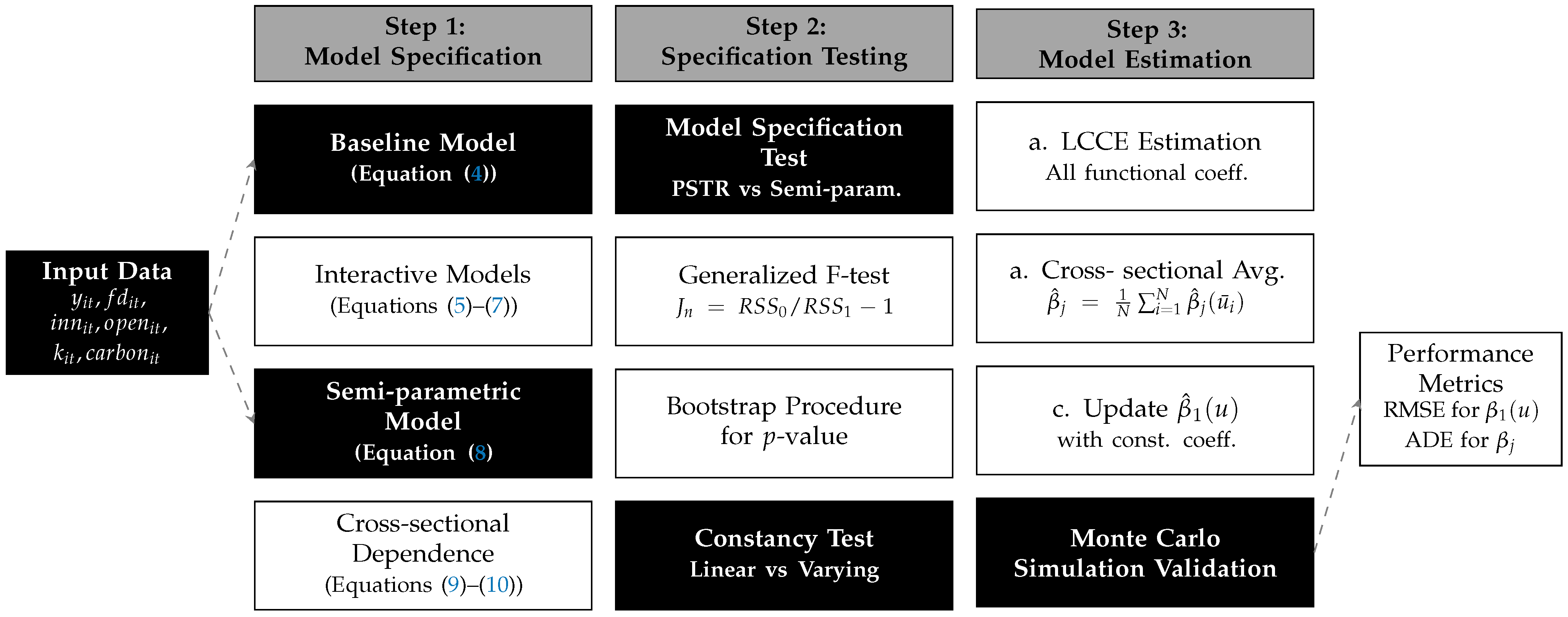
We estimate the semi-parametric model (8) by a three-step procedure. In the first step, we treat all β 1 ( · ) ,   β 2 ,   β 3 ,   β 4 as functional coefficients and employ locally common correlated effects (LCCE) proposed by [24] to get β ^ 1 ( u ) as well as β ^ 2 ( u ) ,   β ^ 3 ( u ) ,   β ^ 4 ( u ) , where u represents a grid point. To achieve parametric convergence rate for the parametric part, in the second step, we choose u ¯ i = 1 T t = 1 T U i t , i = 1 ,   ,   N as grid points, and then calculate the cross-sectional means for the first-step estimators of β 2 to β 4 , which then serve as the final estimates for constant coefficients. That is, we finally get β ^ j = 1 N i = 1 N β ^ j u ¯ i ,   j = 2 ,   3 ,   4 . In the third step, with the help of β ^ j obtained from step 2, we update the estimate of β ^ 1 ( u ) .
We provide a simulation to demonstrate the finite sample performance of the three-step estimation method. The data generating process (DGP) is as follows:
Y i t = β 1 U i t X 1 , i t + β 2 X 2 , i t + γ i + e i t
with
e i t = γ 2 i , 1 f 2 t , 1 + γ 2 i , 2 f 2 t , 2 + ε i t
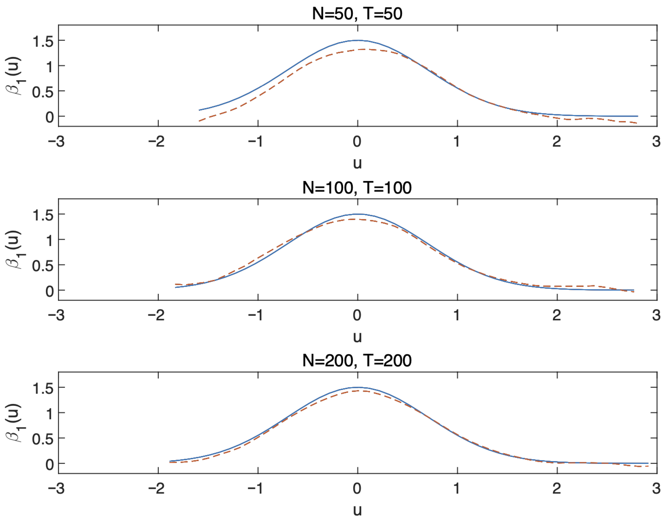
where β 1 U i t = 1.5 exp U i t 2 , Z i t = ( X 1 , i t , X 2 , i t , U i t ) follows (10), and the DGP of factor loadings, common factors and error terms are the same as [58].
We use the same ( N , T ) pairs, kernel function and bandwidth as [24]. The number of Monte Carlo replications is 1000. To evaluate the estimation performance, we use the root mean square error (RMSE):
RMSE = 1 d t = 1 d β ^ 1 u t β 1 u t 2
for the functional coefficient, where ( u 1 , , u d ) are grid points. And for constant coefficients, the absolute deviation error (ADE) is used, and is defined by
ADE = β ^ j β j , j = 2 , 3 , 4 .
Table 2 reports the medians of the RMSE and ADE from 1000 replications for β ^ 1 ( u ) and β ^ 2 . One can observed that the RMSE of the functional-coefficient estimators and the ADE of the constant coefficient estimators decrease rapidly as sample size increases. It shows that the estimators are consistent.
To better demonstrate the estimation performance, we plot the real functional-coefficients (solid line) and the estimated functional-coefficients (dashed line) in Figure 3. We choose ( N , T ) = ( 50 , 50 ) , ( 100 , 100 ) , ( 200 , 200 ) and select the estimation result corresponding to the 500th RMSE value in ascending order among 1000 replications to construct the dashed lines. It can be observed that with an increase in sample size, there is a noticeable improvement in the curve fitting performance.
Figure 4 illustrates the whole methodological steps in the style of [59].

4. Empirical Results and Discussion

4.1. Data and Descriptive Statistics

Given the econometric models, we construct a panel dataset with annual data that contain variables of 30 Chinese mainland provinces (Tibet is excluded) from 1990 to 2022. Following the variable definition in previous influential Chinese study [8], we summarize the data in Table 3. The carbon emissions data are collected from China Emission Accounts and Datasets (CEADs) (part of the CO2 emission data is based on the work of [60,61,62,63,64]), and the rest of the data are from the China statistical Yearbook.

4.2. Results of Baseline Models

We first estimate baseline model (4). Our research focuses mainly on the impact of financial development on economic growth. The first column of Table 4 represents the most restrictive specification. Column (2) through (4) sequentially introduce other primary factors influencing economic growth. All the coefficients of financial development are significantly positive, indicating a discernible facilitative role of financial development in economic growth, consistent with the results of recent Chinese study [8]. For control variables, openness and capital also demonstrate a significant promotion effect on economic growth, whereas innovation exhibits a notable negative impact. This result supports some literature suggesting that innovation plays a double-edged role and may not have a positive impact on the economy [37,38].
To further investigate the impact of financial development on economic growth at different levels of carbon emissions, we estimate the models (5) to (7) with interactive terms. Table 5 displays the results considering the interaction between carbon emissions and financial development. It can be observed that the regressions of the first two interactive terms exhibit an insignificant effect and the third interactive term shows a weakly significant impact, suggesting that the level of carbon emissions does not appear to influence the facilitative role of financial development in economic growth. This contradicts the existing literature [8,65,66]. In fact, relying solely on interactive terms may not accurately capture the genuine relationship between the two variables. For instance, if the interactive effects exhibit non-unidirectional signs, it could lead to the estimated coefficients being rendered insignificant. Therefore, it is necessary to consider a more nuanced model depicting the complex relationship.

4.3. Results of Semi-Parametric Model

We conduct the Pesaran’s Cross-sectional Dependence test on the estimation results of model (4) and find that the test statistic is 29.2557 with a p-value of 0.000 , indicating a highly significant cross-sectional dependence in the dataset.
Next we perform model specification test to compare the PSTR model with our functional-coefficient model. The bootstrap p-value of J n is 0.00 , indicating that we could reject the null hypothesis model, PSTR. This result demonstrates that our model, in addition to being more flexible by not requiring pre-set finite thresholds, also better aligns with real data.
And in order to illustrate the existence of nonlinear relationship in model (8), we conduct a non-parametric constancy test proposed by [24] to examine the null hypothesis H0: β j ( u ) = β j , j = 1 , 2 , 3 , 4 . We vary the bandwidth used in the construction of the test statistic based on the local linear estimation method from 0.4 to 0.8 and the corresponding p-values of the bootstrap test ranging from 0.00 to 0.03. Therefore, we can reject H0 at least at the 5% significance level.
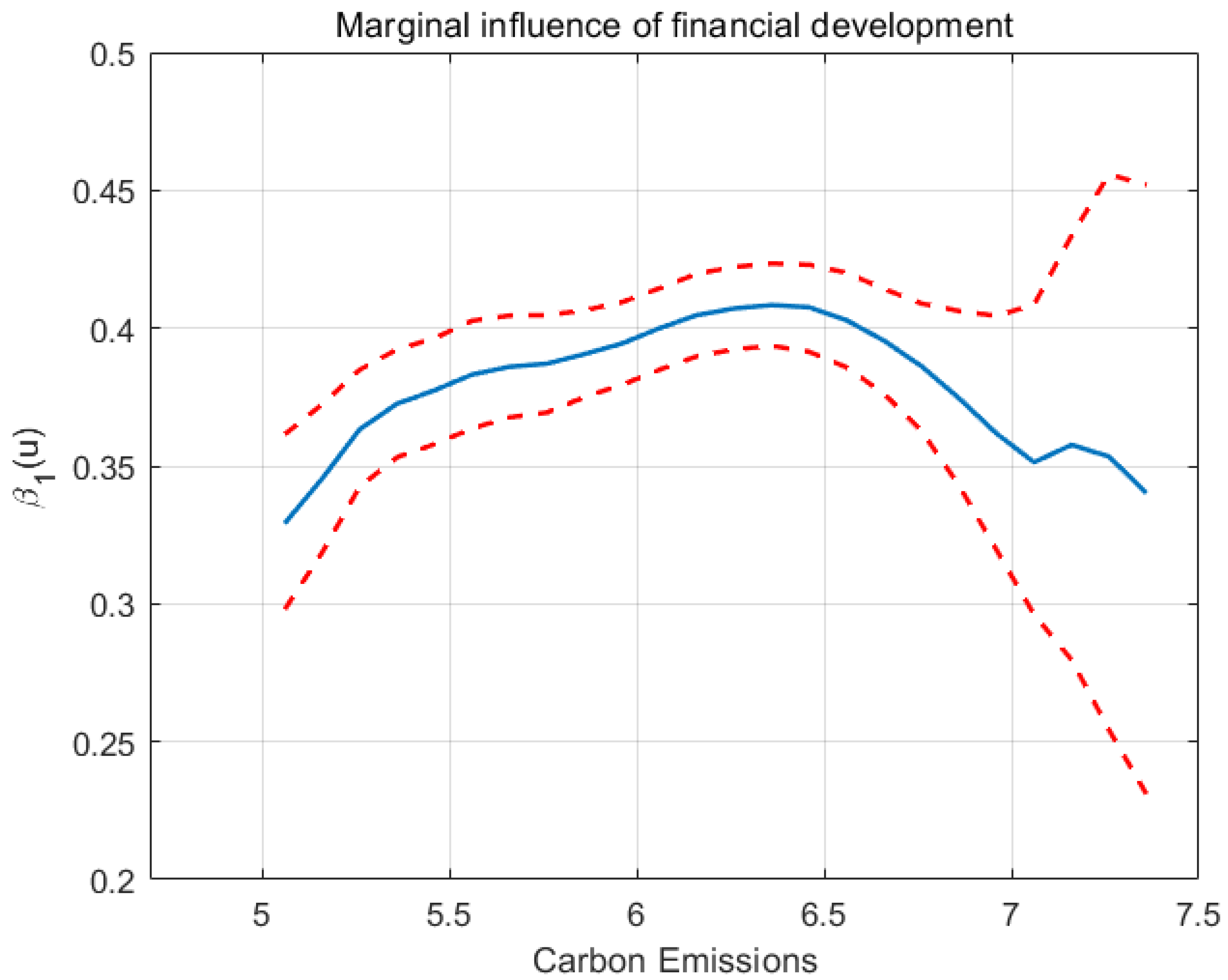
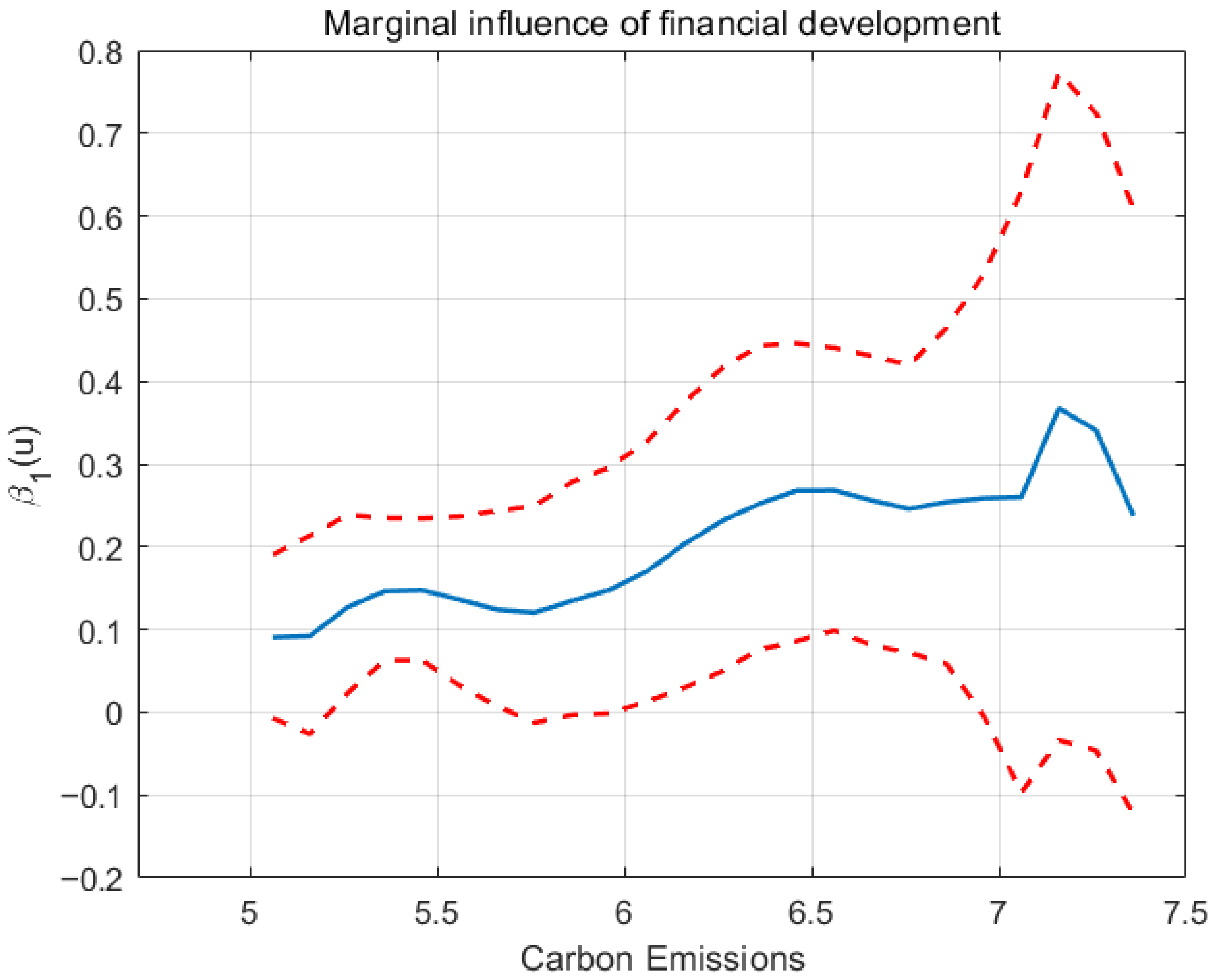
Then, we estimate model (8) and display the estimated results of functional-coefficient and constant coefficient in Figure 5 and Table 6, respectively. The solid line in the figure corresponds to the estimated functional coefficients, while the upper and lower dashed lines represent the 95% confidence intervals. We employ a pointwise bootstrap method to construct the confidence intervals here, considering the slow convergence rate of kernel estimation to its limiting distribution.
Figure 5 provides strong support for H1. It reveals that the growth effect of financial development exhibits a significant nonlinear pattern contingent on carbon emission levels. When carbon emissions remain low, the facilitative impact of financial development on economic growth rises steadily as emissions increase. However, beyond a threshold of approximately 6.4 (in logarithmic terms), the marginal effect of financial development diminishes dramatically with further increases in carbon emissions. This inverted U-shaped relationship can be attributed to the interplay of two competing mechanisms identified in the literature.
On the one hand, rising carbon emissions stimulate green finance development [67], incentivizing greater investment in environmentally sustainable projects and expanding financial intermediation activities that support economic growth. This channel aligns with the theoretical framework of the Environmental Kuznets Curve [19], where initial environmental pressures trigger structural transformation and innovation in the financial sector. On the other hand, elevated carbon emissions exacerbate environmental degradation, increase enterprise-level climate risks, and heighten uncertainty in financial markets [5,22]. These transition and physical risks diminish the effectiveness of financial development in promoting growth by raising the cost of capital and redirecting resources toward risk mitigation rather than productive investment [46].
When carbon emissions are relatively low, the green finance channel predominates, amplifying the positive growth effects of financial development. Conversely, at high emission levels, climate-related risks and market uncertainties dominate, weakening or even reversing this positive relationship. This nonlinear pattern also explains why the estimated coefficients of the interactive terms in models (5) to (7) are not statistically significant: the opposing signs of the interaction effect before and after the turning point cancel each other out in linear specifications, masking the underlying nonlinearity that emerges only through the functional-coefficient approach.
In the results of Table 6, one can observe that the capital has a positive effect on economic growth, while the openness and innovation have no significant positive influence. The reason for the negligible impact of openness may be the transfer of foreign polluting industries to the domestic market, and for innovation, the unreasonable structure of R&D would cause low use efficiency and weak spillover effect on economy [38].
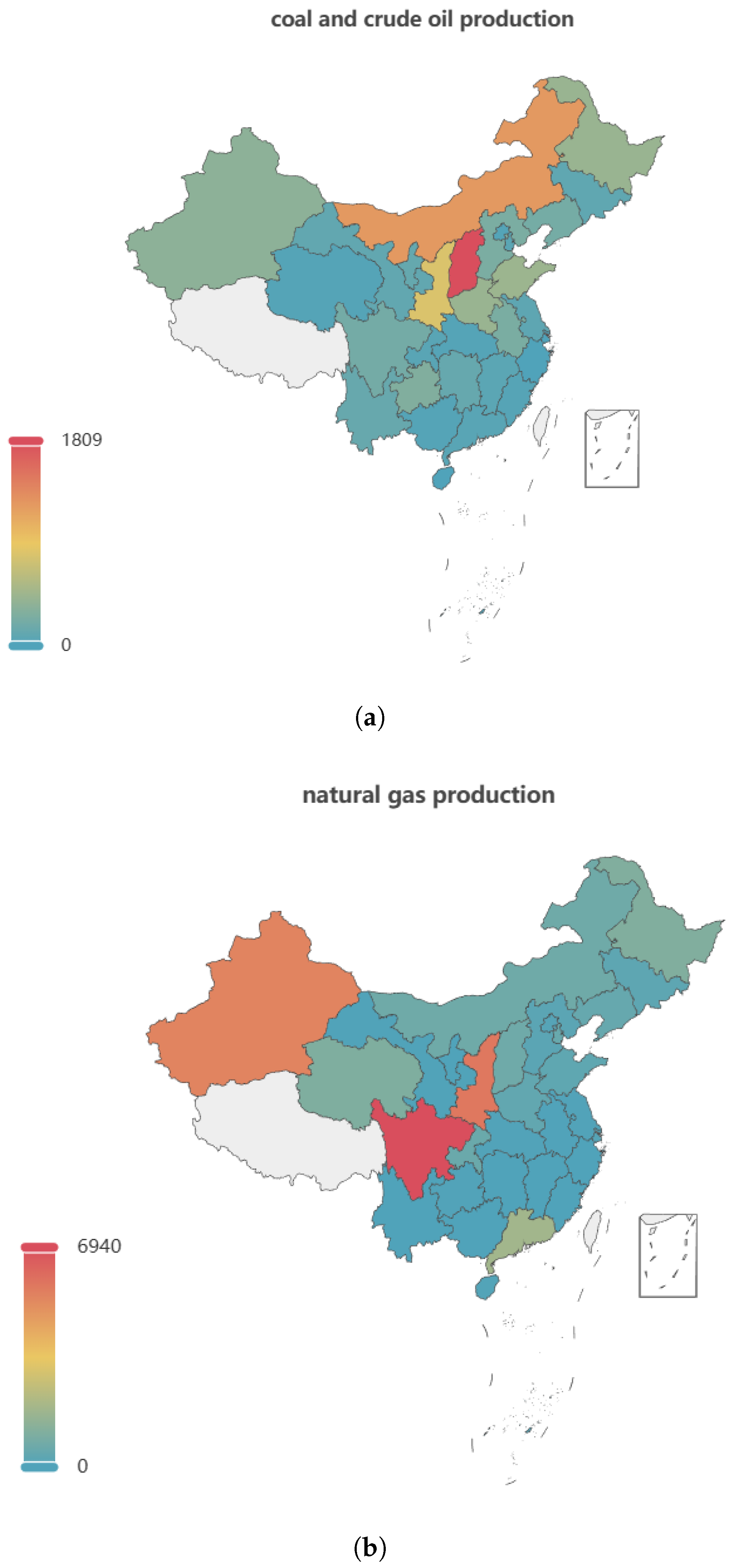
In the following research, in order to examine the heterogeneous characteristics of different regions concerning the impact of financial development on economic growth, we perform group analysis. Considering the disparities in resource allocation among different regions in China, as Figure 6 depicts (data are collected from the Chinese Research Data Service (CNRDS)), it is conceivable that these variations could impact the nonlinear dynamics of financial development effects. According to the ranking of production for coal, crude oil, and natural gas from 1990 to 2020, we divide the regions into three parts: resource-abundant region (Shaanxi, Xinjiang, Heilongjiang, Shandong, Henan, Liaoning, Sichuan, Inner Mongolia, Hebei, Shanxi), resource-moderate region (Guangdong, Jilin, Tianjin, Gansu, Jiangsu, Guizhou, Hubei, Anhui, Chongqing, Ningxia), resource-scarce region (Fujian, Jiangxi, Qinghai, Zhejiang, Beijing, Hainan, Shanghai, Hunan, Guangxi, Yunnan).
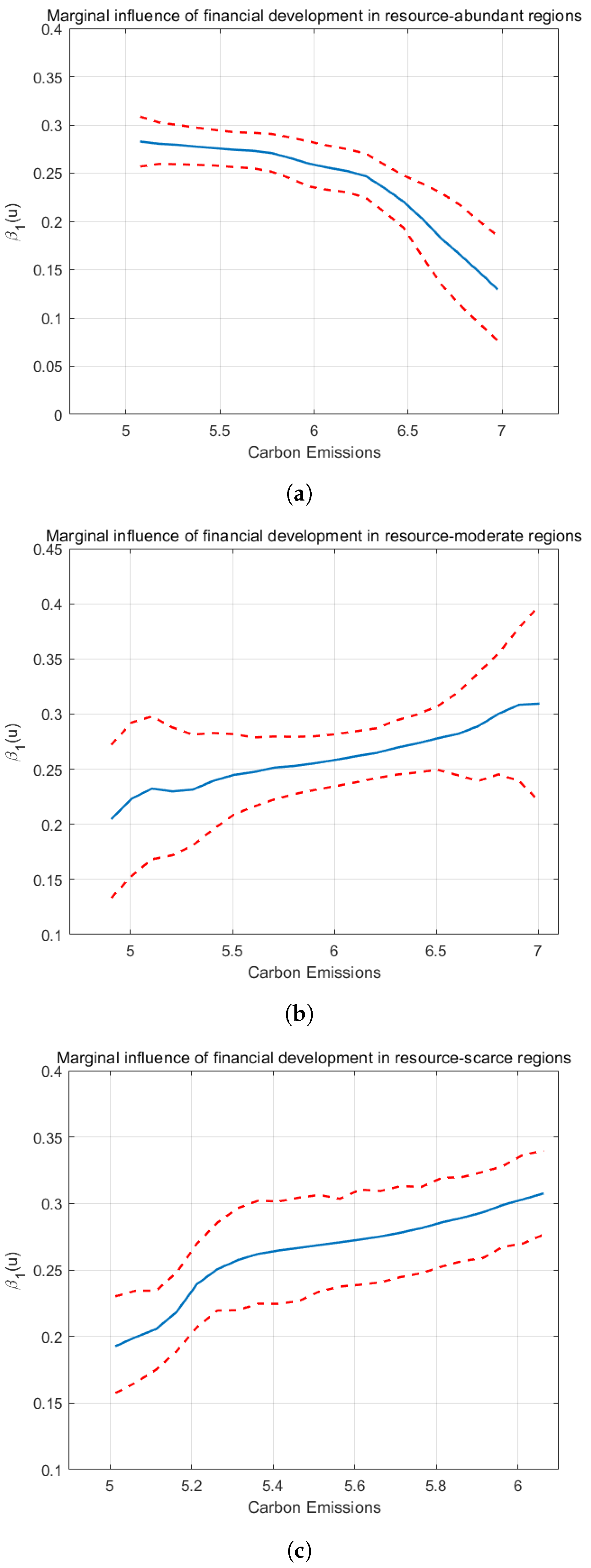
The functional coefficient estimates from the grouped regression are illustrated in Figure 7, revealing that the marginal effect of financial development on economic growth varies substantially across regions with different resource endowments. These results provide strong support for H2. In resource-abundant regions, the marginal effect declines continuously as carbon emissions increase, suggesting that these regions have already surpassed the turning point identified in the aggregate analysis. Nevertheless, financial development maintains a significantly positive growth effect throughout the observed emission range. In contrast, for resource-moderate and resource-scarce provinces, the marginal effect of financial development initially increases with rising carbon emissions, indicating that these regions have yet to reach the threshold beyond which climate-related risks begin to dominate.
These divergent patterns can be attributed to fundamental differences in economic structure, environmental conditions, and policy incentives across resource groups. Resource-abundant regions, heavily reliant on fossil fuel extraction and carbon-intensive industries, face earlier and more severe climate-related risks as emissions accumulate [22]. Their financial systems are disproportionately exposed to transition risks—particularly the threat of stranded assets and declining profitability in carbon-intensive sectors as climate policies tighten [46,48]. Consequently, the negative effects of rising emissions on financial sector effectiveness materialize at lower emission levels, causing the marginal growth impact of financial development to decline even as emissions remain relatively moderate. Moreover, the entrenched political economy of resource extraction in these regions may impede the reallocation of financial capital toward green investments [49], further weakening the green finance channel that could otherwise offset climate risks.
In contrast, resource-moderate and resource-scarce regions exhibit more diversified economic structures with lower baseline carbon intensity. In these regions, the initial increase in emissions may reflect structural transformation and industrialization rather than entrenched dependence on fossil fuels [19,21]. The rise in carbon emissions signals expanding economic activity that stimulates financial deepening and creates demand for green finance solutions [47,67]. Financial institutions in these regions face relatively lower exposure to stranded asset risks and possess greater flexibility to redirect capital toward sustainable investments. Additionally, these provinces may benefit more from national green finance policies and carbon pricing mechanisms, as their economic structures are more amenable to low-carbon transitions [46]. As a result, the green finance channel dominates over climate risk effects at moderate emission levels, amplifying rather than diminishing the growth contribution of financial development.
The contrasting trajectories across resource groups underscore the importance of context-specific policies. Resource-abundant regions require accelerated financial sector reforms to manage transition risks and facilitate capital reallocation away from carbon-intensive activities. Meanwhile, resource-moderate and resource-scarce regions should leverage their structural advantages by strengthening green finance infrastructure before reaching emission thresholds that trigger the negative phase of the nonlinear relationship.

4.4. Robust Test

As the variables used to measure the level of financial development have yet to reach consensus, we replace the measure from domestic credit to the private sector with domestic credit provided by the banking sector (data come from the Statistical Yearbook of each province), following previous related studies [7,41]. We then repeat the estimation process described above to test robustness.
Figure 8 demonstrates that the marginal impact of financial development in China follows a pattern consistent with that observed in Figure 5. Both exhibit an inverted U-shaped trajectory, with the marginal effect initially rising and subsequently declining as carbon emissions increase, although the turning point in Figure 8 occurs at a higher emission level. The estimated constant coefficients presented in Table 7 likewise align with those in Table 6, showing only minor numerical variations. Specifically, both specifications indicate limited impact of trade openness, insignificant effects of innovation, and significantly positive contributions of capital to economic growth. However, to be noticed, financial development causally affects growth through capital allocation efficiency [53,54], though our estimates may still reflect some unresolved reverse causality through province-specific channels.

4.5. Further Discussion

4.5.1. Cross-Country Comparison

While our functional-coefficient model contributes methodologically to understanding the nonlinear relationship among carbon emissions, financial development, and economic growth, our empirical analysis focuses exclusively on China’s provincial data. This approach illuminates China’s internal heterogeneity but leaves questions regarding external validity unresolved. As long as panel data and baseline model assumptions align with those employed in our study, the methodological framework should theoretically hold across contexts. However, systematic comparison with other major emitters—particularly the European Union, the United States, and India—reveals substantial differences in institutional structures, policy environments, and economic characteristics that may fundamentally alter how carbon emissions mediate the finance-growth relationship.
Financial system structure and carbon exposure. China’s bank-dominated financial system, with state-owned commercial banks controlling most of total financial assets, enables rapid capital mobilization but perpetuates financing for carbon-intensive state-owned enterprises [68,69]. The United States operates a market-based system where capital markets account for most of corporate funding, facilitating more flexible reallocation away from high-carbon investments [70,71]. The EU combines strong banking sectors with the world’s most comprehensive green finance taxonomy and mandatory climate disclosure requirements, systematically redirecting capital toward low-carbon activities [72]. India’s bank-dominated system operates at lower financial depth, potentially limiting both green finance benefits and climate risk effects. These structural differences suggest varying magnitudes and timing of the nonlinear patterns observed in China.
Emission trajectories and energy transitions. China remains the world’s largest emitter, driven by coal-fired power and heavy manufacturing, creating substantial stranded asset risks but also strong green finance demand toward its 2060 carbon neutrality target [73]. U.S. emissions have declined since 2007 through natural gas substitution and renewables deployment, reducing legacy financial risks but potentially diminishing green finance urgency [74]. The EU has achieved absolute decoupling with emissions 32% below 1990 levels while GDP grew 70% in 2023, reflecting comprehensive carbon pricing and renewable investments that intensify constraints on residual emissions [75]. India’s rapidly rising emissions from coal-based development, with per capita emissions (1.9 tonnes) below global averages, suggest positioning in the early ascending phase where emissions stimulate green finance without yet triggering substantial climate risks [76].
Climate policy architecture and market incentives. China’s national emissions trading system, launched in 2021, covers only the power sector with carbon prices below USD 20 per ton, a level significantly lower than in Western markets, providing limited reallocation signals. The U.S. lacks federal carbon pricing, relying on fragmented state-level programs that complicate financial risk assessment [77]. The EU operates the most mature carbon market with prices exceeding EUR 100 per ton and comprehensive sectoral coverage, reinforced by the 2023 Carbon Border Adjustment Mechanism, creating strong incentives for financial institutions to internalize climate risks and redirect capital [46]. India has no national carbon pricing, instead using renewable mandates and coal taxation, which may attenuate both green finance stimulus and climate risk channels. China has emerged as the global leader in green finance scale with over USD 4 trillion in green loans and comprehensive central bank guidelines, though definitional inconsistencies persist [78,79]. The EU’s mandatory climate disclosure framework and EU Green Bond Standard create the most systematic institutional support for green finance [80], while U.S. markets operate through voluntary ESG frameworks and India’s initiatives remain nascent [81,82].
Implications for external validity. These cross-country differences suggest that while our methodology provides a generalizable analytical framework, the specific shape and turning points of the nonlinear relationship likely vary substantially across contexts. The EU’s comprehensive policies and integrated green finance architecture may produce sharper nonlinearities with earlier turning points. The U.S.’s fragmented policy landscape may generate more gradual transitions with greater regional variation. India’s lower financial development and nascent climate policies suggest the ascending phase may dominate, with turning points occurring at higher emission levels than China. Rigorous cross-country empirical analysis using comparable data would be necessary to validate these hypotheses and establish boundary conditions for our findings’ external validity.

4.5.2. Other Econometrics Methodology

While our partially linear functional-coefficient model offers a comprehensive framework for analyzing nonlinear relationships among carbon emissions, financial development, and economic growth, alternative panel data approaches provide distinct insights. This section discusses these methodologies and justifies our chosen approach.
Traditional nonlinear models. Threshold regression models [83,84] identify discrete regime switches at endogenously determined emission levels, providing clear policy thresholds where the finance-growth relationship changes. However, they impose abrupt transitions rather than gradual adjustments and struggle with endogeneity when threshold variables correlate with errors [85]. Quantile regression [86,87] reveals heterogeneous effects across growth distributions—whether high-growth provinces respond differently than low-growth ones—but captures distributional rather than structural nonlinearities and typically ignores cross-sectional dependence [88].
Advanced nonlinear models. Panel smooth transition regression (PSTR) [8,89] allows smooth coefficient transitions between regimes via logistic functions, avoiding threshold discontinuities. Yet PSTR assumes homogeneous transitions across provinces and predetermined transition variables, obscuring province-specific paths and endogeneity. Dynamic panel GMM estimators [90,91,92] address simultaneity through lagged instruments, standard for growth regressions with persistent variables. While handling endogeneity and dynamics, the GMM treats endogeneity through instruments rather than modeling its structural source and typically imposes linear or simple polynomial specifications inadequate for complex nonlinearities [93].
Causal inference approaches. Difference-in-differences (DiD) methods [94,95] exploit staggered policy adoption—such as carbon trading pilots or emission regulations—to estimate causal effects by comparing treated and control provinces. Recent advances accommodate heterogeneous treatment effects and dynamic responses [96,97]. However, DiD requires parallel trends assumptions that may fail when provinces follow divergent growth trajectories [98], and China’s overlapping environmental policies create complex treatment patterns violating clean identification [99,100]. Regression discontinuity design (RDD) [101,102] exploits policy thresholds—such as emission-based regulations—to identify local causal effects with minimal assumptions. However, RDD estimates apply only near discontinuities, limiting generalizability [103], and China’s gradualist policies rarely create sharp thresholds suitable for panel RDD [100,104,105]. Geographic thresholds [106,107] are widely used in China’s environmental studies, such as the Qinling Mountains–Huai River line, nearest hydrological monitoring stations, nearest air pollution monitoring stations, and upstream river boundaries. Geographic RD is particularly valuable when policies are assigned based on administrative geography rather than economic characteristics, making the assignment as-good-as-random near boundaries [108]. However, geographic RD faces critical limitations: Chinese regional boundaries often reflect historical economic and institutional differences violating continuity assumptions [109,110]; carbon and financial policies rarely follow sharp geographic boundaries as pilots were implemented in scattered cities rather than contiguous regions; estimates are highly local to boundary areas limiting generalizability [103]; cross-border spillovers through trade and capital flows violate SUTVA [111]; and multiple policies changing simultaneously at boundaries confound attribution [108].
Spatial econometrics. Spatial panel models [112,113], which are widely used in China’s environmental economics studies [114], incorporate geographic spillovers through weight matrices, revealing whether one region’s emissions or finance affects neighbors’ growth via trade, technology, or policy externalities. While addressing geographic correlation, spatial models require pre-specified weights that introduce specification uncertainty [115] and capture only geographic dependence, missing national policies, supply chains, and financial integration that generate non-spatial correlation [116].
Our methodological choice. Our functional-coefficient model addresses these limitations simultaneously. The varying coefficient specification allows smooth, flexible nonlinear functions of emissions without threshold discontinuities or restrictive PSTR forms. Modeling endogeneity through shared factor structures addresses simultaneity without relying on potentially weak external instruments [117], assuming common unobserved forces—national policies, macroeconomic shocks—drive correlated movements in emissions, finance, and growth. The latent factor error structure captures general cross-sectional dependence beyond spatial correlation [25,58], suitable for China’s complex institutional channels. Our test statistic enables formal model selection between functional-coefficient and regime-switching specifications.
However, our approach has limitations: it requires large cross-sections for consistent estimation limiting applicability to regional subsamples [118], assumes endogeneity arises from common shocks rather than province-specific confounders potentially missing local feedback effects [119], and estimates conditional associations adjusted for common factors rather than strict causal treatment effects [120]. While alternatives offer valuable insights—threshold models provide policy cutoffs, DiD identifies treatment effects, spatial models reveal geographic externalities—our framework balances flexibility, endogeneity treatment, and dependence modeling in a unified specification suitable for examining smooth nonlinear relationships across China’s heterogeneous provincial development patterns.
To specify, our model has a strong comparative advantage compared to above methodology. Among methodologies capable of testing the continuous, nonlinear moderating effect of carbon emissions, the interactive fixed effects structure provides the strongest control for endogeneity arising from common shocks and factor-mediated reverse causality. While we cannot achieve the clean causal identification possible with IV/DID/natural experiments, we can rigorously test whether and how the finance-growth relationship varies smoothly across the emissions distribution while controlling for multidimensional unobserved heterogeneity that simpler nonlinear models ignore. This represents a methodological trade-off. We prioritize the ability to document nonlinear moderation mechanisms while maintaining stronger endogeneity controls than alternative nonlinear panel methods, recognizing that we cannot fully resolve all sources of endogeneity. Our factor structure addresses endogeneity from common shocks and factor-mediated reverse causality, but cannot resolve province-specific simultaneity where local growth directly stimulates local financial development through idiosyncratic channels. Readers should interpret our results as conditional on this limitation.

4.5.3. Connections to Frontier Environmental Studies

Our examination of how carbon emissions mediate the finance-growth nexus may engage three emerging research frontiers: carbon finance mechanisms, sustainable investment norms, and the political economy of climate governance.
Carbon finance and green capital allocation. Recent scholarship emphasizes that financial development’s growth effects increasingly depend on environmental performance as carbon pricing and green finance frameworks reshape capital allocation [22,121]. Regulatory frameworks create differentiated capital access based on emissions: low-carbon firms access green bonds and ESG funds at favorable terms while carbon-intensive sectors face divestment pressures [71]. Our functional-coefficient specification captures these dynamics—financial development may accelerate growth in low-emission provinces while constraining high-emission regions facing capital flight and regulatory costs [47].
Sustainable investment norms. ESG integration requires financial actors to price carbon externalities alongside traditional risk-return metrics [122]. This normative shift implies nonlinear effects: emission reductions may unlock green finance premiums and technology spillovers, while crossing thresholds triggers stranded asset risks and reputation penalties [123,124]. Our flexible functional form accommodates such complexity without imposing arbitrary regime boundaries.
Political economy of climate governance. China’s fragmented carbon governance—provincial variation in enforcement stringency and pilot participation—generates heterogeneous finance-growth relationships our model estimates [125,126]. However, political economy critiques caution that financial interests may capture green finance mechanisms, prioritizing profitable carbon markets over genuine emission reductions [127], and North-South tensions constrain developing regions’ finance access under stringent standards [128]. Our findings could imply whether carbon-conditioned finance operates as governance frameworks predict or whether institutional reforms—stricter enforcement, broader carbon pricing, targeted industrial policies—are necessary for finance to serve environmental objectives [129,130].

5. Conclusions and Policy Implications

This paper examines how carbon emissions moderate the finance-growth relationship using a partially linear functional-coefficient model. Our findings reveal nonlinear patterns: financial development’s growth effect initially strengthens as emissions rise but diminishes beyond critical thresholds. Regional heterogeneity emerges across resource endowments—resource-rich provinces exhibit monotonically declining finance-growth effects with emissions, while resource-poor regions show initial intensification before reversal. These patterns suggest carbon emissions exert dual influences: environmental degradation increases uncertainty dampening financial intermediation, while simultaneously stimulating green finance expansion that augments financial scale.
China’s environmental governance has evolved substantially since 2011, encompassing national carbon market pilots (launched 2013, unified 2021), green finance guidelines (2016), and ecological civilization targets in successive Five-Year Plans. Our estimated thresholds likely reflect these institutional shifts—the turning points where finance-growth effects reverse may correspond to pilot carbon market implementation triggering capital reallocation from carbon-intensive sectors, or green credit policies (2012 Green Credit Guidelines) altering bank lending structures. Political economy considerations matter: local government fiscal pressures create incentives to prioritize GDP growth over emission controls, generating enforcement heterogeneity that provincial-level estimates capture.
Based on these findings and institutional realities, we propose targeted policies. First, deepen green financial product innovation—expand green bond markets, environmental rights trading, and climate risk insurance—to channel financial development toward low-carbon growth paths, effectively shifting thresholds rightward. Second, strengthen carbon pricing enforcement and reduce local discretion in implementation to mitigate negative emission externalities that undermine financial intermediation efficiency. Third, design differentiated regional strategies: resource-rich provinces should accelerate industrial restructuring and fossil fuel exit mechanisms, while resource-poor regions prioritize clean technology deployment and green infrastructure finance. Fourth, reform innovation policies to redirect R&D from pollution-intensive process improvements toward genuine green technologies, and enhance FDI screening to prevent the pollution haven effects that our openness coefficients suggest.
Several limitations qualify our conclusions. Conceptually, competing explanations exist for the observed nonlinearities: threshold effects may reflect institutional regime changes rather than emission-driven financial mechanisms, or omitted variables such as energy price shocks could confound the estimated relationships. Methodologically, our identification strategy relies on the baseline Cobb–Douglas extended production function and the latent factor structure. If these assumptions are violated, potential endogeneity problems could arise. For example, province-specific reverse causality remains plausible—economic growth may simultaneously drive both emissions and financial deepening through income effects. Time-sequencing issues emerge because financial development exhibits persistence while emission impacts may operate with lags that our static framework cannot capture. Additionally, the large-N asymptotics required for consistent estimation preclude analyzing shorter panels or smaller regional subsamples. Empirically, provincial aggregation masks within-province heterogeneity across cities and firms where finance-emission dynamics likely operate. Prefecture-level or firm-level data would provide finer resolution but pose measurement challenges for constructing comparable financial development indicators. Externally, China’s unique institutional context—a state-owned financial system, centralized environmental enforcement mechanisms, and export-oriented industrialization patterns—limits the generalizability of our findings to market economies with different governance structures and development stages.
These limitations suggest several future research avenues. While the interactive fixed effects framework provides stronger endogeneity controls than standard nonlinear panel methods, future research could combine our approach with System GMM or identify exogenous policy shocks (e.g., staggered carbon trading pilot rollouts) to further isolate causal mechanisms. Cross-country studies could test whether our findings generalize to other developing economies or reflect China-specific institutional features such as state-owned finance and centralized enforcement. Disaggregated analyses using prefecture-level or firm-level data could identify spatial spillovers and micro-mechanisms masked by provincial aggregation—for instance, how emission regulations alter corporate financing constraints or whether green-certified firms maintain capital cost advantages across emission thresholds.

Author Contributions

Conceptualization, Y.Q. and Z.S.; methodology, Y.Q. and Z.S.; software, Y.Q. and Z.S.; validation, Y.Q. and Z.S.; formal analysis, Y.Q. and Z.S.; investigation, Y.Q. and Z.S.; resources, Y.Q. and Z.S.; data curation, Y.Q. and Z.S.; writing—original draft preparation, Y.Q. and Z.S.; writing—review and editing, Y.Q. and Z.S.; visualization, Y.Q. and Z.S.; supervision, Y.Q.; project administration, Y.Q. and Z.S.; funding acquisition, Y.Q. and Z.S. All authors have read and agreed to the published version of the manuscript.

Funding

This research was funded by the Key Research and Development Program of Sichuan Province, China (Grant No. 2024YFHZ0161).

Institutional Review Board Statement

Not applicable.

Informed Consent Statement

Not applicable.

Data Availability Statement

The data that support the findings of this study are available from the corresponding author upon reasonable request.

Conflicts of Interest

The authors declare no conflicts of interest.

References

  1. King, R.G.; Levine, R. Finance and growth: Schumpeter might be right. Q. J. Econ. 1993, 108, 717–737. [Google Scholar] [CrossRef]
  2. Benhabib, J.; Spiegel, M.M. The role of financial development in growth and investment. J. Econ. Growth 2000, 5, 341–360. [Google Scholar] [CrossRef]
  3. Levine, R. Finance and growth: Theory and evidence. Handb. Econ. Growth 2005, 1, 865–934. [Google Scholar]
  4. Galindo, A.; Schiantarelli, F.; Weiss, A. Does financial liberalization improve the allocation of investment?: Micro-evidence from developing countries. J. Dev. Econ. 2007, 83, 562–587. [Google Scholar] [CrossRef]
  5. Nordhaus, W.D. A review of the Stern review on the economics of climate change. J. Econ. Lit. 2007, 45, 686–702. [Google Scholar] [CrossRef]
  6. Shahbaz, M.; Van Hoang, T.H.; Mahalik, M.K.; Roubaud, D. Energy consumption, financial development and economic growth in India: New evidence from a nonlinear and asymmetric analysis. Energy Econ. 2017, 63, 199–212. [Google Scholar] [CrossRef]
  7. Botev, J.; Égert, B.; Jawadi, F. The nonlinear relationship between economic growth and financial development: Evidence from developing, emerging and advanced economies. Int. Econ. 2019, 160, 3–13. [Google Scholar] [CrossRef]
  8. Li, G.; Wei, W. Financial development, openness, innovation, carbon emissions, and economic growth in China. Energy Econ. 2021, 97, 105194. [Google Scholar] [CrossRef]
  9. Xie, Q.; Bai, D.; Cong, X. Modeling the dynamic influences of economic growth and financial development on energy consumption in emerging economies: Insights from dynamic nonlinear approaches. Energy Econ. 2022, 116, 106404. [Google Scholar] [CrossRef]
  10. Usman, M.; Jahanger, A.; Makhdum, M.S.A.; Balsalobre-Lorente, D.; Bashir, A. How do financial development, energy consumption, natural resources, and globalization affect Arctic countries’ economic growth and environmental quality? An advanced panel data simulation. Energy 2022, 241, 122515. [Google Scholar] [CrossRef]
  11. Ajeigbe, K.B.; Ganda, F. The impact of pollution and carbon emission control on financial development, environmental quality, and economic growth: A global analysis. Sustainability 2024, 16, 8748. [Google Scholar] [CrossRef]
  12. Lashof, D.A.; Ahuja, D.R. Relative contributions of greenhouse gas emissions to global warming. Nature 1990, 344, 529–531. [Google Scholar] [CrossRef]
  13. Matthews, H.D.; Gillett, N.P.; Stott, P.A.; Zickfeld, K. The proportionality of global warming to cumulative carbon emissions. Nature 2009, 459, 829–832. [Google Scholar] [CrossRef]
  14. Khalfaoui, R.; Tiwari, A.K.; Khalid, U.; Shahbaz, M. Nexus between carbon dioxide emissions and economic growth in G7 countries: Fresh insights via wavelet coherence analysis. J. Environ. Plan. Manag. 2023, 66, 31–66. [Google Scholar] [CrossRef]
  15. Choudhury, T.; Kayani, U.N.; Gul, A.; Haider, S.A.; Ahmad, S. Carbon emissions, environmental distortions, and impact on growth. Energy Econ. 2023, 126, 107040. [Google Scholar] [CrossRef]
  16. Freire-González, J.; Vivanco, D.F.; Jin, Y. World economies’ progress in decoupling from CO2 emissions. Sci. Rep. 2024, 14, 71101. [Google Scholar] [CrossRef]
  17. Rigas, A. The impact of CO2 emissions and climate on economic growth and productivity: International evidence. Rev. Dev. Econ. 2024, 28, e13075. [Google Scholar] [CrossRef]
  18. Guo, C.; Yi, X. China’s Economic Growth under the “Dual Carbon” Target: Influencing Mechanisms, Trend Characteristics and Countermeasures Suggestions. Economist 2022, 7, 24–33. [Google Scholar] [CrossRef]
  19. Grossman, G.M.; Krueger, A.B. Economic growth and the environment. Q. J. Econ. 1995, 110, 353–377. [Google Scholar] [CrossRef]
  20. Cole, M.A. Trade, the pollution haven hypothesis and the environmental Kuznets curve: Examining the linkages. Ecol. Econ. 2004, 48, 71–81. [Google Scholar] [CrossRef]
  21. Dinda, S. Environmental Kuznets curve hypothesis: A survey. Ecol. Econ. 2004, 49, 431–455. [Google Scholar] [CrossRef]
  22. Battiston, S.; Mandel, A.; Monasterolo, I.; Schütze, F.; Visentin, G. A climate stress-test of the financial system. Nat. Clim. Change 2017, 7, 283–288. [Google Scholar] [CrossRef]
  23. Jiang, Y. Understanding openness and productivity growth in China: An empirical study of the Chinese provinces. China Econ. Rev. 2011, 22, 290–298. [Google Scholar] [CrossRef]
  24. Cai, Z.; Fang, Y.; Xu, Q. Testing capital asset pricing models using functional-coefficient panel data models with cross-sectional dependence. J. Econom. 2022, 227, 114–133. [Google Scholar] [CrossRef]
  25. Bai, J. Panel data models with interactive fixed effects. Econometrica 2009, 77, 1229–1279. [Google Scholar] [CrossRef]
  26. Shaw, E.S. Financial Deepening in Economic Development; Oxford University Press: Oxford, UK, 1973. [Google Scholar]
  27. Fry, M.J. Money and Capital or Financial Deepening in Economic Development? J. Money Credit. Bank. 1978, 10, 464–475. [Google Scholar] [CrossRef]
  28. Jung, W.S. Financial development and economic growth: International evidence. Econ. Dev. Cult. Change 1986, 34, 333–346. [Google Scholar] [CrossRef]
  29. Levine, R. Financial development and economic growth: Views and agenda. J. Econ. Lit. 1997, 35, 688–726. [Google Scholar]
  30. Rousseau, P.L.; Wachtel, P. What is happening to the impact of financial deepening on economic growth? Econ. Inq. 2011, 49, 276–288. [Google Scholar] [CrossRef]
  31. Beck, R.; Georgiadis, G.; Straub, R. The finance and growth nexus revisited. Econ. Lett. 2014, 124, 382–385. [Google Scholar] [CrossRef]
  32. Law, S.H.; Singh, N. Does too much finance harm economic growth? J. Bank. Financ. 2014, 41, 36–44. [Google Scholar] [CrossRef]
  33. Ibrahim, M.; Alagidede, P. Nonlinearities in financial development–economic growth nexus: Evidence from sub-Saharan Africa. Res. Int. Bus. Financ. 2018, 46, 95–104. [Google Scholar] [CrossRef]
  34. Romer, P.M. Endogenous technological change. J. Political Econ. 1990, 98, S71–S102. [Google Scholar] [CrossRef]
  35. Eaton, J.; Kortum, S. Trade in ideas Patenting and productivity in the OECD. J. Int. Econ. 1996, 40, 251–278. [Google Scholar] [CrossRef]
  36. Lebel, P. The role of creative innovation in economic growth: Some international comparisons. J. Asian Econ. 2008, 19, 334–347. [Google Scholar] [CrossRef]
  37. Zhang, J.; Chang, Y.; Zhang, L.; Li, D. Do technological innovations promote urban green development?–A spatial econometric analysis of 105 cities in China. J. Clean. Prod. 2018, 182, 395–403. [Google Scholar] [CrossRef]
  38. Song, X.; Zhou, Y.; Jia, W. How do economic openness and R&D investment affect green economic growth?–Evidence from China. Resour. Conserv. Recycl. 2019, 146, 405–415. [Google Scholar]
  39. Yanikkaya, H. Trade openness and economic growth: A cross-country empirical investigation. J. Dev. Econ. 2003, 72, 57–89. [Google Scholar] [CrossRef]
  40. Papageorgiou, C. Trade as a threshold variable for multiple regimes. Econ. Lett. 2002, 77, 85–91. [Google Scholar] [CrossRef]
  41. Menyah, K.; Nazlioglu, S.; Wolde-Rufael, Y. Financial development, trade openness and economic growth in African countries: New insights from a panel causality approach. Econ. Model. 2014, 37, 386–394. [Google Scholar] [CrossRef]
  42. Azam, M. Does environmental degradation shackle economic growth? A panel data investigation on 11 Asian countries. Renew. Sustain. Energy Rev. 2016, 65, 175–182. [Google Scholar] [CrossRef]
  43. Ghosh, S. Examining carbon emissions economic growth nexus for India: A multivariate cointegration approach. Energy Policy 2010, 38, 3008–3014. [Google Scholar] [CrossRef]
  44. Zhai, S.; Song, G. Exploring carbon emissions, economic growth, energy and R&D investment in China by ARDL approach. In Proceedings of the 2013 21st International Conference on Geoinformatics, Kaifeng, China, 20–22 June 2013; pp. 1–6. [Google Scholar]
  45. Chen, C.; Pinar, M.; Stengos, T. Renewable energy consumption and economic growth nexus: Evidence from a threshold model. Energy Policy 2020, 139, 111295. [Google Scholar] [CrossRef]
  46. European Commission. Proposal for a Regulation of the European Parliament and of the Council Establishing a Carbon Border Adjustment Mechanism (CBAM); COM (2021) 564 Final; European Commission: Brussels, Belgium, 2021. [Google Scholar]
  47. Carney, M. Breaking the Tragedy of the Horizon—Climate Change and Financial Stability; Speech at Lloyd’s of London; Bank of England: London, UK, 2015. [Google Scholar]
  48. Campiglio, E.; Dafermos, Y.; Monnin, P.; Ryan-Collins, J.; Schotten, G.; Tanaka, M. Climate change challenges for central banks and financial regulators. Nat. Clim. Change 2018, 8, 462–468. [Google Scholar] [CrossRef]
  49. Carbon Pricing Leadership Coalition. Report of the High-Level Commission on Carbon Pricing and Competitiveness. World Bank, 2019. License: CC BY-NC-ND 3.0 IGO. Available online: http://hdl.handle.net/10986/32419 (accessed on 1 December 2025).
  50. Lu, W.; Huang, J.; Musshoff, O. Climate threshold, financial hoarding and economic growth. Appl. Econ. 2015, 47, 4535–4548. [Google Scholar] [CrossRef]
  51. Yan, Z.; Zou, B.; Du, K.; Li, K. Do renewable energy technology innovations promote China’s green productivity growth? Fresh evidence from partially linear functional-coefficient models. Energy Econ. 2020, 90, 104842. [Google Scholar] [CrossRef]
  52. Munir, Q.; Lean, H.H.; Smyth, R. CO2 emissions, energy consumption and economic growth in the ASEAN-5 countries: A cross-sectional dependence approach. Energy Econ. 2020, 85, 104571. [Google Scholar] [CrossRef]
  53. Lucas, R.E., Jr. On the mechanics of economic development. J. Monet. Econ. 1988, 22, 3–42. [Google Scholar] [CrossRef]
  54. Romer, P.M. Capital Accumulation in the Theory of Long Run Growth; Working Paper No. 123; University of Rochester—Center for Economic Research (RCER): Rochester, NY, USA, 1988. [Google Scholar]
  55. Belazreg, W.; Mtar, K. Modelling the causal linkages between trade openness, innovation, financial development and economic growth in OECD Countries. Appl. Econ. Lett. 2020, 27, 5–8. [Google Scholar] [CrossRef]
  56. Cai, Z.; Tiwari, R.C. Application of a local linear autoregressive model to BOD time series. Environmetrics 2000, 11, 341–350. [Google Scholar] [CrossRef]
  57. Cai, Z.; Fan, J.; Yao, Q. Functional-coefficient regression models for nonlinear time series. J. Am. Stat. Assoc. 2000, 95, 941–956. [Google Scholar] [CrossRef]
  58. Pesaran, M.H. Estimation and inference in large heterogeneous panels with a multifactor error structure. Econometrica 2006, 74, 967–1012. [Google Scholar] [CrossRef]
  59. de Melo, G.A.; Peixoto, M.G.M.; Barbosa, S.B.; Mendonça, M.C.A.; Nogueira, T.H.; Guerra, J.B.S.O.D.A.; de Castro Júnior, L.G.; Serrano, A.L.M.; Ferreira, L.O.G. Fuel flow logistics: An empirical analysis of performance in a network of gas stations using principal component analysis and data envelopment analysis. J. Adv. Manag. Res. 2024, 21, 605–626. [Google Scholar] [CrossRef]
  60. Shan, Y.; Guan, D.; Zheng, H.; Ou, J.; Li, Y.; Meng, J.; Mi, Z.; Liu, Z.; Zhang, Q. China CO2 emission accounts 1997–2015. Sci. Data 2018, 5, 170201. [Google Scholar] [CrossRef]
  61. Shan, Y.; Liu, J.; Liu, Z.; Xu, X.; Shao, S.; Wang, P.; Guan, D. New provincial CO2 emission inventories in China based on apparent energy consumption data and updated emission factors. Appl. Energy 2016, 184, 742–750. [Google Scholar] [CrossRef]
  62. Shan, Y.; Huang, Q.; Guan, D.; Hubacek, K. China CO2 emission accounts 2016–2017. Sci. Data 2020, 7, 54. [Google Scholar] [CrossRef]
  63. Guan, Y.; Shan, Y.; Huang, Q.; Chen, H.; Wang, D.; Hubacek, K. Assessment to China’s recent emission pattern shifts. Earth’s Future 2021, 9, e2021EF002241. [Google Scholar] [CrossRef]
  64. Xu, J.; Guan, Y.; Oldfield, J.; Guan, D.; Shan, Y. China carbon emission accounts 2020–2021. Appl. Energy 2024, 360, 122837. [Google Scholar] [CrossRef]
  65. Narayan, P.K.; Saboori, B.; Soleymani, A. Economic growth and carbon emissions. Econ. Model. 2016, 53, 388–397. [Google Scholar] [CrossRef]
  66. Rajpurohit, S.S.; Sharma, R. Impact of economic and financial development on carbon emissions: Evidence from emerging Asian economies. Manag. Environ. Qual. Int. J. 2021, 32, 145–159. [Google Scholar] [CrossRef]
  67. Cogan, D.G. Corporate Governance and Climate Change: The Banking Sector; Ceres Report; Ceres: Boston, MA, USA, 2008. [Google Scholar]
  68. Allen, F.; Qian, J.; Qian, M. Law, finance, and economic growth in China. J. Financ. Econ. 2005, 77, 57–116. [Google Scholar] [CrossRef]
  69. Song, Z.; Storesletten, K.; Zilibotti, F. Growing like China. Am. Econ. Rev. 2011, 101, 196–233. [Google Scholar] [CrossRef]
  70. Levine, R. Bank-based or market-based financial systems: Which is better? J. Financ. Intermediat. 2002, 11, 398–428. [Google Scholar] [CrossRef]
  71. Krueger, P.; Sautner, Z.; Starks, L.T. The importance of climate risks for institutional investors. Rev. Financ. Stud. 2020, 33, 1067–1111. [Google Scholar] [CrossRef]
  72. European Commission. EU Taxonomy for Sustainable Activities. 2020. Available online: https://finance.ec.europa.eu/sustainable-finance/tools-and-standards/eu-taxonomy-sustainable-activities_en (accessed on 1 December 2025).
  73. He, G.; Lin, J.; Sifuentes, F.; Liu, X.; Abhyankar, N.; Phadke, A. Rapid cost decrease of renewables and storage accelerates the decarbonization of China’s power system. Nat. Commun. 2020, 11, 2486. [Google Scholar] [CrossRef] [PubMed]
  74. U.S. Environmental Protection Agency. Inventory of U.S. Greenhouse Gas Emissions and Sinks: 1990–2022. 2024. Available online: https://www.epa.gov/ghgemissions/inventory-us-greenhouse-gas-emissions-and-sinks (accessed on 1 December 2025).
  75. European Environment Agency. Trends and Projections in Europe 2025. 2025. Available online: https://www.eea.europa.eu/en/analysis/publications/trends-and-projections-in-europe-2025 (accessed on 1 December 2025).
  76. Gupta, N.C.; Tanwar, R.; Dipesh; Kaushik, A.; Singh, R.; Patra, A.K.; Sar, P.; Khakharia, P. Perspectives on CCUS deployment on large scale in India: Insights for low carbon pathways. Carbon Capture Sci. Technol. 2024, 12, 100195. [Google Scholar] [CrossRef]
  77. Rabe, B.G. Can We Price Carbon? MIT Press: Cambridge, MA, USA, 2018. [Google Scholar]
  78. International Institute of Green Finance. China Green Finance Research Report 2024. Central University of Finance and Economics, 2024. Available online: https://iigf.cufe.edu.cn/info/1014/9340.htm (accessed on 1 December 2025).
  79. Nedopil, C.; Dordi, T.; Weber, O. The nature of global green finance standards—Evolution, differences, and three models. Sustainability 2021, 13, 3723. [Google Scholar] [CrossRef]
  80. European Commission. Strategy for Financing the Transition to a Sustainable Economy. 2021. Available online: https://finance.ec.europa.eu/publications/strategy-financing-transition-sustainable-economy_en (accessed on 1 December 2025).
  81. Bos, K.; Gupta, J. Stranded assets and stranded resources: Implications for climate change mitigation and global sustainable development. Energy Res. Soc. Sci. 2021, 56, 101215. [Google Scholar] [CrossRef]
  82. Bhattacharya, A.; Meltzer, J.P.; Oppenheim, J.; Qureshi, Z.; Stern, N. Delivering on Sustainable Infrastructure for Better Development and Better Climate. Brookings Institution. 2016. Available online: https://www.brookings.edu/articles/delivering-on-sustainable-infrastructure-for-better-development-and-better-climate/ (accessed on 1 December 2025).
  83. Hansen, B.E. Threshold effects in non-dynamic panels: Estimation, testing, and inference. J. Econom. 1999, 93, 345–368. [Google Scholar] [CrossRef]
  84. Hansen, B.E. Sample splitting and threshold estimation. Econometrica 2000, 68, 575–603. [Google Scholar] [CrossRef]
  85. Caner, M.; Hansen, B.E. Instrumental variable estimation of a threshold model. Econom. Theory 2004, 20, 813–843. [Google Scholar] [CrossRef]
  86. Koenker, R. Quantile regression for longitudinal data. J. Multivar. Anal. 2004, 91, 74–89. [Google Scholar] [CrossRef]
  87. Canay, I.A. A simple approach to quantile regression for panel data. Econom. J. 2011, 14, 368–386. [Google Scholar] [CrossRef]
  88. Galvao, A.F.; Kato, K. Smoothed quantile regression for panel data. J. Econom. 2016, 193, 92–112. [Google Scholar] [CrossRef]
  89. Fok, D.; Van Dijk, D.; Franses, P.H. A multi-level panel STAR model for US manufacturing sectors. J. Appl. Econom. 2005, 20, 811–827. [Google Scholar] [CrossRef]
  90. Arellano, M.; Bond, S. Some tests of specification for panel data: Monte Carlo evidence and an application to employment equations. Rev. Econ. Stud. 1991, 58, 277–297. [Google Scholar] [CrossRef]
  91. Blundell, R.; Bond, S. Initial conditions and moment restrictions in dynamic panel data models. J. Econom. 1998, 87, 115–143. [Google Scholar] [CrossRef]
  92. Levine, R.; Loayza, N.; Beck, T. Financial intermediation and growth: Causality and causes. J. Monet. Econ. 2000, 46, 31–77. [Google Scholar] [CrossRef]
  93. Eberhardt, M.; Presbitero, A.F. This Time They’re Different: Heterogeneity and Nonlinearity in the Relationship between Debt and Growth; IMF Working Paper; IMF: Washington, DC, USA, 2013. [Google Scholar]
  94. Athey, S.; Imbens, G.W. Design-based analysis in difference-in-differences settings with staggered adoption. J. Econom. 2022, 226, 62–79. [Google Scholar] [CrossRef]
  95. Callaway, B.; Sant’Anna, P.H. Difference-in-differences with multiple time periods. J. Econom. 2021, 225, 200–230. [Google Scholar] [CrossRef]
  96. Sun, L.; Abraham, S. Estimating dynamic treatment effects in event studies with heterogeneous treatment effects. J. Econom. 2021, 225, 175–199. [Google Scholar] [CrossRef]
  97. de Chaisemartin, C.; D’Haultfœuille, X. Two-way fixed effects estimators with heterogeneous treatment effects. Am. Econ. Rev. 2020, 110, 2964–2996. [Google Scholar] [CrossRef]
  98. Roth, J.; Sant’Anna, P.H.C.; Bilinski, A.; Poe, J. What’s trending in difference-in-differences? A synthesis of the recent econometrics literature. J. Econom. 2023, 235, 2218–2244. [Google Scholar] [CrossRef]
  99. Goodman-Bacon, A. Difference-in-differences with variation in treatment timing. J. Econom. 2021, 225, 254–277. [Google Scholar] [CrossRef]
  100. Wen, S.; Wang, Z.; Zhang, L.; Liu, X. The Green Function of Finance: From Doctrinal History to Theoretical Modelling. Manag. World 2025, 41, 175–197. [Google Scholar] [CrossRef]
  101. Lee, D.S.; Lemieux, T. Regression discontinuity designs in economics. J. Econ. Lit. 2010, 48, 281–355. [Google Scholar] [CrossRef]
  102. Cattaneo, M.D.; Idrobo, N.; Titiunik, R. A Practical Introduction to Regression Discontinuity Designs; Cambridge University Press: Cambridge, UK, 2019. [Google Scholar]
  103. Angrist, J.D.; Pischke, J.S. Mostly Harmless Econometrics; Princeton University Press: Princeton, NJ, USA, 2009. [Google Scholar]
  104. Hausman, C.; Rapson, D.S. Regression discontinuity in time: Considerations for empirical applications. Annu. Rev. Resour. Econ. 2018, 10, 533–552. [Google Scholar] [CrossRef]
  105. Xiao, Q.; Yin, J. Research on the Impact of ESG Informal Institutions on the Financial Sustainable Development of Manufacturing Enterprises—Based on Regression Discontinuity Design. Stat. Manag. 2025, 40, 4–14. [Google Scholar]
  106. Chen, Y.; Li, X.; Zhang, X. Does the Increase in Pollution Levy Hinder Enterprise Exports—A Study Based on Geographic Regression Discontinuity Method. China Econ. Q. 2025, 25, 121–136. [Google Scholar]
  107. Luo, Y.; Liu, S.; Zhang, Y. Taking Responsibility or Free-Riding: How Does Air Pollution Affect Corporate ESG Performance? Account. Res. 2025, 1, 44–58. [Google Scholar]
  108. Keele, L.J.; Titiunik, R. Geographic boundaries as regression discontinuities. Political Anal. 2015, 23, 127–155. [Google Scholar] [CrossRef]
  109. Baum-Snow, N.; Brandt, L.; Henderson, J.V.; Turner, M.A.; Zhang, Q. Roads, railroads, and decentralization of Chinese cities. Rev. Econ. Stat. 2017, 99, 435–448. [Google Scholar] [CrossRef]
  110. Dell, M. The persistent effects of Peru’s mining mita. Econometrica 2010, 78, 1863–1903. [Google Scholar] [CrossRef]
  111. Barreca, A.I.; Lindo, J.M.; Waddell, G.R. Heaping-induced bias in regression-discontinuity designs. Econ. Inq. 2016, 54, 268–293. [Google Scholar] [CrossRef]
  112. Elhorst, J.P. Spatial Econometrics: From Cross-Sectional Data to Spatial Panels; Springer: Cham, Switzerland, 2014. [Google Scholar]
  113. LeSage, J.; Pace, R.K. Introduction to Spatial Econometrics; CRC Press: Boca Raton, FL, USA, 2009. [Google Scholar]
  114. Li, J.; Wu, Y. A Review of Frontier Theories, Methods and Applied Research in Spatial Econometrics. Contemp. Econ. Manag. 2024, 46, 30–41. [Google Scholar]
  115. LeSage, J.P.; Pace, R.K. The biggest myth in spatial econometrics. Econometrics 2014, 2, 217–249. [Google Scholar] [CrossRef]
  116. Yu, J.; De Jong, R.; Lee, L.F. Estimation for spatial dynamic panel data with fixed effects. J. Econom. 2015, 167, 16–37. [Google Scholar] [CrossRef]
  117. Bazzi, S.; Clemens, M.A. Blunt instruments: Avoiding common pitfalls in identifying the causes of economic growth. Am. Econ. J. Macroecon. 2013, 5, 152–186. [Google Scholar] [CrossRef]
  118. Su, L.; Jin, S. Sieve estimation of panel data models with cross section dependence. J. Econom. 2012, 169, 34–47. [Google Scholar] [CrossRef]
  119. Moon, H.R.; Weidner, M. Linear regression for panel with unknown number of factors as interactive fixed effects. Econometrica 2015, 83, 1543–1579. [Google Scholar] [CrossRef]
  120. Imbens, G.W.; Rubin, D.B. Causal Inference in Statistics, Social, and Biomedical Sciences; Cambridge University Press: Cambridge, UK, 2015. [Google Scholar]
  121. Bolton, P.; Kacperczyk, M. Do investors care about carbon risk? J. Financ. Econ. 2021, 142, 517–549. [Google Scholar] [CrossRef]
  122. Schoenmaker, D.; Schramade, W. Principles of Sustainable Finance; Oxford University Press: Oxford, UK, 2019. [Google Scholar]
  123. Semieniuk, G.; Campiglio, E.; Mercure, J.F.; Volz, U.; Edwards, N.R. Low-carbon transition risks for finance. Wiley Interdiscip. Rev. Clim. Change 2021, 12, e678. [Google Scholar] [CrossRef]
  124. Mercure, J.F.; Pollitt, H.; Viñuales, J.E.; Edwards, N.R.; Holden, P.B.; Chewpreecha, U.; Salas, P.; Sognnaes, I.; Lam, A.; Knobloch, F. Macroeconomic impact of stranded fossil fuel assets. Nat. Clim. Change 2018, 8, 588–593. [Google Scholar] [CrossRef]
  125. Lo, A.Y. Challenges to the development of carbon markets in China. Clim. Policy 2016, 16, 109–124. [Google Scholar] [CrossRef]
  126. Wang, P.; Wu, W.; Zhu, B.; Wei, Y. Examining the impact factors of energy-related CO2 emissions using the STIRPAT model in Guangdong Province, China. Appl. Energy 2013, 106, 65–71. [Google Scholar] [CrossRef]
  127. Newell, P.; Paterson, M. Climate Capitalism: Global Warming and the Transformation of the Global Economy; Cambridge University Press: Cambridge, UK, 2010. [Google Scholar]
  128. Ciplet, D.; Roberts, J.T.; Khan, M.R. Power in a Warming World: The New Global Politics of Climate Change and the Remaking of Environmental Inequality; MIT Press: Cambridge, MA, USA, 2015. [Google Scholar]
  129. Mazzucato, M. Mission Economy: A Moonshot Guide to Changing Capitalism; Harper Business: New York, NY, USA, 2021. [Google Scholar]
  130. Stern, N. A time for action on climate change and a time for change in economics. Econ. J. 2022, 132, 1259–1289. [Google Scholar] [CrossRef]
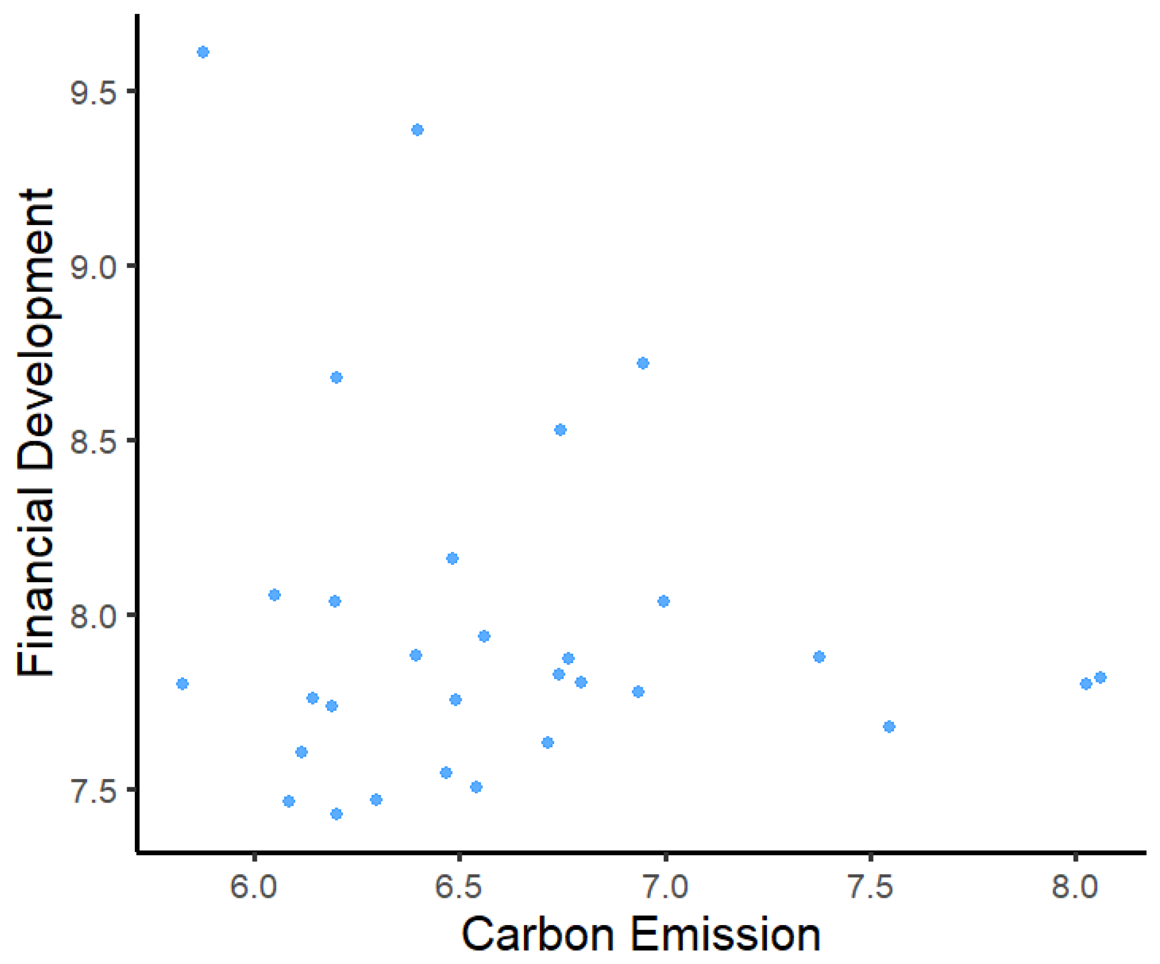
Figure 1. The scatter plot of provincial carbon emissions and financial development in 2022. Specific variable definitions and data sources can be found in Section 4.
Sustainability 17 11249 g001
Figure 2. Conceptual figure for theory and methodology foundation.
Sustainability 17 11249 g002
Figure 3. Estimation results of functional coefficient. Solid lines represent the true function curve, while dashed lines depict the estimated curves of the functional-coefficient. To construct the dashed lines, we select the estimation results corresponding to the 500th RMSE value in ascending order among 1000 replications.
Sustainability 17 11249 g003
Figure 4. Methodological framework for semi-parametric panel data analysis with cross-sectional dependence. The framework consists of three main steps: (Step 1) Model specification, progressing from baseline linear models to semi-parametric models with cross-sectional dependence. (Step 2) Specification testing, including model comparison tests and constancy tests. (Step 3) Model estimation using a three-step LCCE procedure and Monte Carlo validation.
Sustainability 17 11249 g004
Figure 5. Estimation results of functional-coefficient in semi-parametric model (8). The X-axis represents carbon emissions (log of CO2 emissions in million tons). The Y-axis represents the marginal effect of financial development on economic growth. Solid lines represent estimation of functional-coefficient in model (8), and the upper and lower dashed lines represent the 95% bootstrap confidence intervals. The figure illustrates the nonlinear inverted-U shape relation between carbon emissions and the impact of financial development on economic growth.
Sustainability 17 11249 g005
Figure 6. Distribution of total coal, crude oil, and natural gas production in China from 1990 to 2022. (a) Distribution of total raw coal and crude oil production in China from 1990 to 2022 (unit: 10 million tons). (b) Distribution of total natural gas production in China from 1990 to 2022 (unit: billion cubic meters).The closer the color is to the top of the spectrum, the higher the total output of that province; conversely, the lower the total output.The figure shows that the total output of oil, gas, and coal is higher in central China, northern China, and western regions, while the total output is lower in eastern regions.
Sustainability 17 11249 g006
Figure 7. Marginal influence of financial development in different regions. The X-axis represents carbon emissions (log of CO2 emissions in million tons). The Y-axis represents the marginal effect of financial development on economic growth. Solid lines represent estimation of functional-coefficient in model (8), and the upper and lower dashed lines represent the 95% bootstrap confidence intervals. (a) Resource-abundant region. (b) Resource-moderate region. (c) Resource-scarce region. The figures illustrate that the marginal effect of financial development on economic growth declines as carbon emissions increase in resource-abundant regions, while it increases with rising carbon emissions in resource-moderate and resource-scarce regions.
Sustainability 17 11249 g007
Figure 8. Estimation results of functional-coefficient in semi-parametric model (8) after changing measure method of financial development. The X-axis represents carbon emissions (log of CO2 emissions in million tons). The Y-axis represents the marginal effect of financial development on economic growth. Solid lines represent estimation of functional-coefficient in model (8), and the upper and lower dashed lines represent the 95% bootstrap confidence intervals. The robust analysis figure also illustrates the nonlinear inverted-U shape relation between carbon emissions and the impact of financial development on economic growth.
Sustainability 17 11249 g008
Table 1. Summary of main studies on financial development, carbon emissions and economic growth.
Research ThemeRepresentative StudiesMethodologyKey Findings
Financial Development and Growth
Classical positive view[1,26,29]Regression analysisFinancial development promotes growth through improved resource allocation
and investment
Challenged relationships[30,31,32]Threshold modelsFinance-growth linkage has weakened; negative impacts beyond certain thresholds
Carbon Emissions and Growth
Mixed direct effects[42,43,44]Panel/time-series analysisNegative, neutral, or positive effects depending on context and time horizon
Interaction Effects: Carbon Emissions, Finance, and Growth
Theoretical mechanisms[5,19,22]Theoretical modelsEmissions reflect structural transformation but create transition and physical risks at high levels
Policy factors[46,47,48]Policy/regulatory analysisCarbon pricing and green finance policies redirect capital away from high-carbon sectors
Methodological Approaches to Nonlinearity
Nonlinear models[8,32,45,51]Threshold/smooth transition/functional-
coefficient models
Nonlinear relationships exist but cross-sectional dependence
often ignored
Note: This table summarizes key empirical and theoretical studies, highlighting the evolution from linear finance-growth models to complex nonlinear frameworks incorporating environmental factors.
Table 2. Median of RMSE and ADE of estimator.
N / T 50100200
β ^ 1 ( u ) β ^ 2 β ^ 1 ( u ) β ^ 2 β ^ 1 ( u ) β ^ 2
500.11440.04360.08670.03230.06710.0274
1000.08940.02860.06450.02140.05150.0200
2000.06790.02170.05030.01610.03890.0136
Table 3. Definitions and descriptive statistics of variables.
VariableDefinitionMinMeanMaxS.D.Obs
c a r b o n CO2 emissions in million tons3.57946.01968.06150.7252990
yReal GDP per capita6.67979.606112.13921.2492990
o p e n Deposits and loans per capita1.91945.886710.12391.8590990
f d Imports and exports per capita2.30735.93299.61081.5251990
i n n Number of patents per 1,000,000 people−0.97502.60716.83331.7825990
kCapital stock per capita1.57335.73348.77371.7668990
Note: All data are logarithmized.
Table 4. Estimation results for the baseline model (4) (dependent variable: y).
Variable(1)(2)(3)(4)
f d 0.8297 ***0.7532 ***0.7765 ***0.5079 ***
(0.0028)(0.0090)(0.0122)(0.0199)
o p e n 0.0859 ***0.0886 ***0.0702 ***
(0.0097)(0.0097)(0.0087)
i n n −0.0241 **−0.0247 **
(0.0085)(0.0075)
k 0.2350 ***
(0.0145)
Note: Standard errors are in parentheses; *** and **, denote p < 0.01 and p < 0.05 , respectively.
Table 5. Estimation results for models with interactive term (dependent variable: y).
Variable(5)(6)(7)
f d i t × c a r b o n i t 0.0024
(0.0021)
f d i t × c a r b o n g a p i t 0.0191
(0.0173)
f d i t × D i t −0.0037 *
(0.0018)
f d 0.4969 ***0.4969 ***0.4998 ***
(0.0222)(0.0222)(0.0202)
o p e n 0.0694 ***0.0694 ***0.0735 ***
(0.0087)(0.0087)(0.0088)
i n n −0.0260 ***−0.0260 ***−0.0215 **
(0.0076)(0.0076)(0.0076)
k0.2301 ***0.2301 ***0.2417 ***
(0.0152)(0.0152)(0.0149)
Note: Standard errors are in parentheses; ***, **, * denote p < 0.01 , p < 0.05 , p < 0.10 , respectively.
Table 6. Estimation results of constant coefficient in semi-parametric model (8).
VariableCoefficient Estimation95% Confidence Interval
o p e n 0.0647( 0.0143 , 0.1443 )
i n n 0.0126 ( 0.1099 , 0.0847 )
k0.3375( 0.0645 , 0.6104 )
Note: The confidence intervals here are obtained by averaging the upper and lower bounds of the bootstrap confidence intervals across grid points u.
Table 7. Estimation results of constant coefficient in semi-parametric model (8) after changing measure method of financial development.
VariableCoefficient Estimation95% Confidence Interval
o p e n 0.1338(0.0004, 0.2668)
i n n 0.0372( 0.1051 , 0.1787)
k0.5113(0.3549, 0.6689)
Note: The confidence intervals here are obtained by averaging the upper and lower bounds of the bootstrap confidence intervals across grid points u.
Disclaimer/Publisher’s Note: The statements, opinions and data contained in all publications are solely those of the individual author(s) and contributor(s) and not of MDPI and/or the editor(s). MDPI and/or the editor(s) disclaim responsibility for any injury to people or property resulting from any ideas, methods, instructions or products referred to in the content.