Article

Economic Dynamics of Informal Output in Romania: An ARDL Approach to Policy, Growth, and Institutional Sustainability

1
Department of Economic Informatics and Cybernetics, Bucharest University of Economic Studies, 010552 Bucharest, Romania
2
Department of Information Systems, Åbo Akademi University, Tuomiokirkontori 3, 20500 Turku, Finland
*
Author to whom correspondence should be addressed.
Sustainability 2025, 17(24), 10920; https://doi.org/10.3390/su172410920 (registering DOI)
Submission received: 8 November 2025 / Revised: 24 November 2025 / Accepted: 4 December 2025 / Published: 6 December 2025

Abstract

In this paper we investigate the short-run and long-run determinants of the informal economy in Romania using Dynamic General Equilibrium (DGE)-based estimates of informal output as the dependent variable. An ARDL model is used to analyze macroeconomic and institutional variables for Romania during the period of 1995–2023, including inflation (INF), primary net lending/borrowing (NLB), the political stability index (PSI), interest payments (INTPAY), gross domestic product per capita (GDP), and self-employment (SEMP). The findings show that inflation, fiscal balance, political stability, interest payments, and GDP per capita have a short- and long-run impact on informal output. In the long run, a 1% increase in inflation raises informal output by 0.03%, while a 1% rise in GDP per capita reduces it by 0.29%. The error correction term suggests a rapid adjustment speed of 79% toward the long-run equilibrium. These findings suggest that institutional reforms, sustained economic growth, and stable macroeconomic policies play an important role in reducing informality and promoting sustainable economic resilience in Romania.

1. Introduction

Many developing and emerging markets have a sizable informal economy, which poses problems for fiscal sustainability, labor market dynamics, and overall economic development [1,2]. The informal sector has persisted in Romania due to institutional factors, labor market structures, and macroeconomic fluctuations [3,4]. To understand the determinants of informal output is important for designing policies aimed at formalization, enhancing tax compliance, and promoting inclusive growth [5,6].
In the context of financial studies, the informal economy directly affects fiscal sustainability. The shrinking tax base, increase in deficits, and distortion of fiscal policies contribute to its impact on fiscal sustainability. According to recent literature, a high share of the market being vested in the informal economy reduces the efficiency of public revenue collection and constrains the government’s ability to implement countercyclical policies [7,8]. Consequently, understanding informal dynamics has become essential, not only for economic growth but also for fiscal stability and long-term financial resilience.
Economic research has given the shadow economy and the informal economy plenty of attention due to their complex relationships with fiscal policy, economic development, and institutional governance [9,10]. Despite their frequent interchangeability, there is a minor distinction between these terms.
Any legal, market-based production of goods and services that is deliberately concealed from public authorities in order to avoid paying taxes, following rules, or abiding by labor standards is referred to as the “shadow economy”. Unregistered economic activity is part of the informal economy and is driven more by a lack of access to institutions and markets than by law disobedience [11]. Understanding the difference in these concepts is important because of their impact on social justice and macroeconomic stability.
The study of the informal economy is important due to its implications for economic growth, government revenue, and labor market dynamics. The informal sector represents a significant share of economic activities in many developing and emerging economies, including Romania. During a recession, the informal economy sector acts as a buffer, offering income opportunities for the unemployed. At the same time, it lowers labor protection standards and limits the efficiency of monetary and fiscal policies. Government incomes are undermined through tax evasion. In the same way, similar difficulties arise from the shadow economy, which further distorts official economic data. To create policies that promote formalization and simultaneously foster inclusive growth, a deeper understanding of the dynamics of informality is important for policymakers. Another relevant channel is that of monetary and fiscal policies. A large informal economy weakens monetary transmission mechanisms through an increased preference for cash and reduced participation in the formal financial system. From a fiscal policy perspective, the need for loan financing increases, which is reflected in the evolution of the primary balance (NLB) and interest payments (INTPAY). These complex interactions define the risk profile of emerging economies, such as Romania, and justify a dedicated econometric analysis.
The originality of our research lies in our understanding of the determinants, consequences, and policy implications of the informal and shadow economies. Previous research has focused specifically on tax evasion or labor market informality. Recent studies have acknowledged that informality is a complex social phenomenon impacted by macroeconomic volatility, institutional weaknesses, and socio-political factors [1,12]. Romania’s post-transition structure, EU integration, and its institutional history influence its informal economy. By means of the Autoregressive Distributed Lag (ARDL) model, we examine both short-term fluctuations and long-term equilibrium relationships. We study how inflation, fiscal balance, political stability, interest payments, GDP per capita, and self-employment influence informality.
The main contribution of this study addresses the integration of the formal economy into a sustainable macroeconomic framework. This framework connects fiscal balance, institutional quality, and social inclusion. Combining the ARDL Model with dynamic simulations through Local Projections, our research captures both the short-term and long-term effects of macroeconomic and institutional variables on informality. The results of our study can provide an empirical basis for the creation of policies that formalize economic resilience and institutional trust. These are closely linked to Sustainable Development Goals 8 (Decent work and economic growth) and 16 (Peace, justice and strong institutions).
Specifically, our research develops a unified framework that details how macroeconomic stability, institutional quality, and labor market structure affect the size of the informal economy in Romania. Unlike previous research, which has analyzed these connections individually or in international contexts, our study offers an integrated approach, using an ARDL model together with local projections to capture both short-term adjustment dynamics and long-term equilibria. Also, the application of an informality indicator based on the DGE model is an essential contribution, as it allows for a more precise estimation of uncontrolled activities than the usual techniques, which are based on cash demand. This integrated approach offers a new vision of how fiscal policies, political and institutional stability, and the post-accession structural context in relation to the European Union influence informality in Romania.
Understanding the determinants of the shadow economy is important to understand the economic dynamics of emerging nations, such as Romania. The shadow economy has a big impact on fiscal sustainability, labor market structures, and institutional trust. There are still research gaps in how institutional and macroeconomic factors interact to shape informal economic activities. Given its economic transition, EU membership, and its integration into global markets, Romania makes an interesting case for such a study. Its varying levels of political stability and macroeconomic performance create an appropriate context for investigating the determinants of informal output. Inflation, GDP per capita, and interest payments are well-known drivers of informal output.
Businesses can function informally to avoid higher expenses brought on by inflation, which reduces purchasing power. A higher GDP per capita encourages formalization by increasing the associated returns. By influencing borrowing and spending patterns, interest payments can also influence informality. The size of the informal sector is determined by institutional quality, namely, political stability and fiscal balance. Uncertainty caused by political unrest can push economic activities underground. Primary net lending/borrowing as a measure of fiscal balance points to the credibility of a government. Institutional trust and compliance with the formal economy can be enhanced by a positive fiscal balance. Another factor essential for understanding the informal economy is self-employment. Self-employment can be associated with informality, since it indicates financial vulnerability. In modern economies, self-employment symbolizes entrepreneurial activity.
Another aspect to be studied is how quickly Romania’s informal economy responds to macroeconomic shocks. Slower responses might point to more serious structural issues, while rapid adjustments suggest a productive policy environment. The study of this behavior can reveal the Romanian economy’s resilience and how efficient measures to reduce informality are.
In this study, we pose the following research questions.
RQ1: How do macroeconomic variables such as inflation, GDP per capita, and interest payments influence the informal economy in Romania in both the short and long run?
RQ2: Can institutional factors, such as political stability and fiscal balance, determine the size of Romania’s informal economy?
RQ3: Does self-employment contribute to the reduction in informality, and how does it reflect broader labor market transformations?
RQ4: What is the speed of adjustment of Romania’s informal economy toward long-run equilibrium following macroeconomic shocks?
The empirical analysis is guided by these four research questions. We use a Dynamic General Equilibrium (DGE)-based measure of informal output. By means of an ARDL model, we study its determinants in both short- and long-run equilibrium relationships.
In a broader context, the analysis provides insight into how fiscal discipline, political stability, and inflation can act synergistically to reduce pressure on government revenues and ensure a sustainable path for public finances. For this reason, the study has direct relevance for the development of strategies for formalization, fiscal consolidation, and a reduction in macroeconomic vulnerabilities.
This study is structured as follows. Section 2 reviews the relevant literature and highlights the research gap regarding Romania’s informal economy. Section 3 presents the data and variable structure, and the methodological framework, including the ARDL specification and cointegration approach. Section 4 presents the empirical results concerning the dynamics of Romania’s informal economy within a sustainable development framework. Section 5 discusses the empirical findings in relation to the formulated research questions (RQ1–RQ4) and interprets the short-run, long-run, and dynamic effects of macroeconomic and institutional factors on the informal economy. Section 6 concludes with policy implications and recommendations for reducing informality in Romania.

2. Research Gap and Literature Review

The literature review discusses the main theoretical perspectives and empirical findings on the informal economy, establishing the context for our results.

2.1. Recent Contributions to the Study of Informality

2.1.1. Institutional Quality and Informality

Recent research highlights the fundamental role of institutions in shaping the size of the informal economy. Gillanders and Parviainen [13] show that, in European economies, corruption and weak control institutions generate an environment in which undeclared activities proliferate, suggesting that informality functions as an adaptive response to the inadequacy of governance mechanisms. Their results highlight the importance of administrative transparency and institutional quality in reducing incentives for evasion.
Another direction is provided by Alm and Embaye [14], who use the cash demand approach to estimate the size of the underground economy in over 100 countries. They highlight that the persistence of cash demand is strongly influenced by institutional variables such as tax law enforcement efforts. Their study confirms that informality is present in all economies analyzed, with high values in countries with weak institutions and insufficient sanctioning mechanisms.
Medina and Schneider [7] make a cross-country analysis and prove that a decrease in the informal sector corresponds to improvements in the rule of law and governance quality. In line with Kaufmann and Kraay [15], their results imply that institutional trust is a main driver of informal economic activity.
An institutional channel increasingly discussed in the recent literature is the digitalization of public administration. Elbahnasawy [16] shows that e-government initiatives—by reducing bureaucracy, increasing transparency, and simplifying the interaction between citizens and the administration—significantly limit the space for informal activities. These results are relevant for emerging economies such as Romania, where institutional modernization and fiscal digitalization are determinant factors for formalization.

2.1.2. Macroeconomic Volatility and Informal Economy

Macroeconomic volatility is one of the main structural factors that stimulate informal activities in emerging economies. Nedić et al. [17] emphasized the importance of macroeconomic stability and discovered that inflation volatility leads to higher levels of informality in developing economies. Periods of inflation deter formal sector participation because of the higher associated operational costs and regulatory burdens.
Dabla-Norris and Koeda [18] make an important contribution to this framework, demonstrating that the implementation of credible inflation targeting strategies significantly reduces the motivation for informal activities. Monetary stability improves the predictability of the economic environment and encourages transactions through formal channels, reducing reliance on informal mechanisms. This direction is consistent with the perspective of Schneider and Enste [11]. In their work, they argue that macroeconomic uncertainty—whether it stems from price volatility, output shocks, or fiscal imbalances—amplifies agents’ preference for parallel activities that are less exposed to regulation.
At the intersection of macroeconomic instability and institutional weakness, Huynh and Nguyen [19] show that developing Asian economies experience a sharp increase in the shadow economy when corruption overlaps with ineffective fiscal policies. The combination of macroeconomic uncertainty and poor governance creates an environment in which tax compliance is perceived as costly and of little benefit, and informality becomes an adaptive strategy.

2.1.3. Fiscal Policy and Informality

Recent literature emphasizes the importance of fiscal policy in influencing informality. According to Torgler and Schneider [20], credible fiscal policies improve institutional trust and formal sector participation. The types of government decentralization and their impact on institutional quality are analyzed by Goel and Saunoris [21]. A better institutional quality and some forms of decentralization can reduce the size of the informal economy.

2.1.4. Labor Market Dynamics and Self-Employment

Oviedo et al. [22] analyze in detail the role of self-employment in the informal economy. They believe that self-employment represents formal entrepreneurial activity rather than informal subsistence work in economies experiencing structural changes. Better credit availability, simplified company registration procedures, and institutional frameworks are the main forces behind this change. These results agree with Williams and Round [23], who claim that formal entrepreneurship is a major factor in the decline of informality.

2.1.5. Technological Advancement and Informality

In recent years, the effect of digitalization on informality has become recognized. Nguyen et al. [24] found that increased internet use corresponds to a decrease in the shadow economy, according to data from 114 economies between 2002 and 2015. It follows that formal economic participation is encouraged when internet penetration rises, transparency improves, and transaction costs drop. This trend is influenced by digital payment systems. Frost et al. [25] examined 101 economies from 2014 to 2019. A 1% increase in digital payment use is associated with a 0.1% rise in per capita GDP growth over two years and a 0.06% reduction in informal employment. Digital payments increase financial inclusion and provide secure transaction methods, reducing informal cash-based activities.
Digital platforms have a role in formalizing labor markets. Digital labor market platforms can lower search frictions in both formal and informal labor, improve employer–worker matching, and create job opportunities, according to Krichewsky-Wegener [26]. E-government initiatives reduce informality by facilitating access to information and administrative processes. The adoption of e-government services implies a reduction in informal employment and the shadow economy’s GDP share [27].
Significant research gaps exist with regard to the dynamic interactions between macroeconomic policies and informal economic activities in Romania. Sometimes, the role of institutional variables like political stability has been neglected in such studies. There is a lack of research that reflects the distinct economic and institutional characteristics of Romania. This study addresses these gaps by using DGE-based estimates of informal output and applying the ARDL model to differentiate short-term dynamics from long-term trends.

2.1.6. Informality, Economic Sustainability, and Institutional Resilience

The informal economy is increasingly being analyzed from the perspective of economic sustainability and resilience. Reducing informality directly contributes to fiscal sustainability, decent work (SDG 8), and institutional integrity (SDG 16). A sustainable economic system requires the efficient allocation of resources between the formal and informal sectors, preventing tax base erosion and social inequalities. In emerging economies such as Romania, combating informality becomes not only a matter of economic efficiency but also an essential condition for sustainable and inclusive growth. Recent studies provide a complex perspective on how the informal economy interacts with sustainability, the environment, and institutional resilience.
Sarkar, Hasan, and Saha [28] examine the economic resilience of street vendors in Dhaka during the COVID-19 pandemic and highlight that the informal economy plays a crucial role in securing livelihoods during times of crisis. The authors identify four dimensions of resilience—prevention, protection, response, and recovery—emphasizing that public policies should target skills development, access to finance, and gradual formalization to strengthen socio-economic resilience.
In a similar manner, Fridayani et al. [29] demonstrate that digitalization and environmental practices can strengthen the resilience of the informal sector. The study, which was conducted in Yogyakarta, Indonesia, shows that digital platforms and recycling initiatives support informal entrepreneurs to increase their productivity and become more sustainable, while also providing relevant lessons for economic inclusion policies.
The link between the informal economy and energy sustainability is explored further by Yazdanie et al. [30], who show that the expansion of the informal economy, climate migration, and rising temperatures can significantly influence urban energy planning, especially in developing economies. The results for Accra, Ghana, confirm that an expanded informal economy can amplify energy demand and make it more difficult to achieve decarbonization goals, suggesting the need for integrated environmental, energy, and informal economy policies. Cartwright and Igudia [31] argue, from a methodological perspective, that the study of the informal economy must combine quantitative and qualitative methods. The lack of consistent statistical data reduces the ability to fully understand the complexity of the phenomenon, and qualitative approaches can complement econometric analysis by providing a more nuanced view of the adaptation and behavior of informal economic agents. Regarding the interaction between environmental regulations and the informal economy, Abid et al. [32] show, for a sample of 25 countries in Sub-Saharan Africa, that weak environmental regulation favors both the expansion of the informal economy and an increase in pollution. These results confirm the existence of an environmental Kuznets curve and highlight that strengthening the regulatory framework is a necessary condition for reducing both pollution and informality. Nica et al. [33] analyzed the effects of financial contagion on human well-being in Romania, revealing that financial instability can undermine the progress toward sustainable development by exacerbating economic inequalities and reducing social welfare. Their findings highlight the necessity of integrating financial resilience into regional development policies to enhance overall sustainability and societal well-being.

2.2. Research Gap, Conceptual Framework, and Contribution

Although recent literature provides a broad understanding of the relationship between institutional quality, fiscal policy, and the informal economy, most studies remain focused on developed countries or on cross-country samples. In the case of Romania, research is limited and rarely captures the macroeconomic and institutional dimensions simultaneously. For example, indicators such as political stability or primary net lending/borrowing are often omitted from empirical models, although they directly reflect fiscal sustainability and the degree of institutional trust. Thus, there is a gap in the specialized literature on the dynamic analysis of the interaction between fiscal policy, macroeconomic stability, and the dimension of informality in emerging economies in Eastern Europe.
From a methodological point of view, many studies have used static models (Ordinary Least Square [34,35,36], structural equation model [37], panel fixed effects [32,38]) that do not capture short-term adjustment and long-term equilibrium behaviors. However, the Autoregressive Distributed Lag (ARDL) model allows for a clear separation of these effects and the analysis of their cointegration in a dynamic framework [39,40]. In addition, estimating informality through Dynamic General Equilibrium (DGE)-based output provides a more precise measure of informal activity than traditional indicators (such as cash demand) [41,42]. Thus, the study proposes a more robust methodological perspective on the dynamics of informality in Romania.
A key contribution of the research is the simultaneous integration of the fiscal (through NLB and INTPAY) and institutional (through PSI) dimensions in the analysis of the informal economy. This approach allows us to understand how fiscal sustainability and political stability influence the degree of economic formalization. Therefore, the study provides an empirical basis for designing fiscal consolidation and inclusive growth policies, with an impact on Romania’s macroeconomic resilience.
Overall, these recent contributions suggest that economic informality, sustainability, and institutional resilience are interdependent phenomena. Digitalization, environmental policies, and financial inclusion can strengthen the capacity of emerging economies to transform the informal sector into a vector of sustainable growth. In this context, the present study extends the literature by analyzing the dynamics of the informal economy in Romania through the lens of macroeconomic and institutional sustainability, offering an original perspective on the mechanisms of adaptation and formalization in the long term.
In summary, the main contribution of the paper is threefold: (1) it provides a dynamic assessment of the determinants of the informal economy in Romania, in the short and long term; (2) it uses a more comprehensive set of macroeconomic and institutional variables than previous studies; and (3) it provides relevant empirical evidence for the formulation of fiscal and institutional policies aimed at reducing informality. Through this approach, the research extends the specialized literature and provides an integrated perspective on the links between the informal economy, fiscal balance, and sustainable economic growth.

2.3. Conceptual Framework and Theoretical Mechanisms of Informal Output Dynamics

In Figure 1, we have designed the conceptual architecture that describes the mechanisms through which institutional, macroeconomic, fiscal, and structural variables influence the size of the informal economy in Romania. On the left, institutional quality, measured by the Political Stability Index (PSI), affects governance, trust in institutions, and the level of fiscal compliance, reducing incentives for informal activities. In the central area, macroeconomic stability (INF, GDP per capita) and fiscal sustainability (NLB, INTPAY) determine the cost of living and operating costs of firms, respectively, as well as fiscal pressure and budgetary constraints. These effects converge towards decreasing participation in the formal sector and increasing the motivation for evasion and undeclared activities. On the right, structural labor market conditions, through self-employment (SEMP), generate forms of informality related to micro-activities and subsistence work. All these channels together lead to variations in Informal Output, measured by DGE estimates, which represents the cumulative result of the interaction between institutions, macro-fiscal policies, and the structure of the labor market.
Our conceptual framework from Figure 1 explicitly focuses on informal output (DGE-based), referring exclusively to legal but unreported productive activities. This distinction is essential because the shadow economy also includes illegal activities, which are not relevant for macro-institutional transmission channels such as inflation, fiscal policy, or political stability [43,44]. Therefore, our empirical model correctly isolates the formal–informal margin of legal production, consistent with institutional and macroeconomic mechanisms.

3. Data Collection and Methodology

The data in Table 1 have been collected from various sources for the period of 1995–2023. The variables presented in Table 1 capture the multidimensional nature of sustainable economic development. This is made possible by correlating macroeconomic stability, institutional quality, and labor market dynamics. The inclusion of the DGE shows the structural dimension of economic sustainability. A high level of the informal economy undermines fiscal revenues, social protection, and fair competition. The INF, INTPAY, and NLB indicators describe macro-fiscal sustainability, determining the capacity of an economy to maintain stable and inclusive growth. GDP captures the economic pillar of sustainability. PSI shows the institutional dimension and reinforces the idea that trust, governance, and security help achieve long-term sustainable development goals. SEMP encompasses the social and entrepreneurial dimension of sustainability. It highlights labor market flexibility, but also the transition to formalized activities based on innovation. Variable selection follows standard criteria in the informality literature, emphasizing macroeconomic, fiscal, institutional, and labor market determinants. In constructing the database, differences in measurement units (percentages, index scores, and level variables) and in the methodological background of each indicator were harmonized through logarithmic transformation and alignment to a common annual frequency. The data construction process also involved verifying consistency across sources, especially for fiscal indicators (NLB, INTPAY) and institutional measures (PSI), which may undergo periodic methodological revisions. As noted in the literature, DGE-based estimates of informal output inherently involve model-based uncertainty, while PSI relies on perception-based assessments. These aspects were taken into account when interpreting the empirical results.
Based on these variables, the analysis employs an ARDL model to examine both short- and long-term relationships, complemented by Local Projections [51] to assess the dynamic effects of macroeconomic and institutional shocks over time.
The dependent variable in the study is the DGE-based estimate of informal output, expressed as a share of official GDP. The DGE time series is extracted from the World Bank Informal Economy Database, which contains data for over 160 economies using the framework developed by Elgin and Oztunali [52], Ihrig and Moe [53], and updated by Elgin et al. [45]. The DGE model assumes that households allocate labor between formal and informal production. Informal output is derived from equilibrium conditions of productivity, taxation, and institutional characteristics [54].
The DGE indicator is obtained using a structural model applied identically for all years, to allow comparability [55]. There is some degree of uncertainty in the estimates that depend on sectoral productivity, taxation, and behavioral responses. The DGE values should be seen as theoretically supported proxies rather than precise observations of informal activity, as stated in World Bank documentation. Despite these drawbacks, survey-based informal economy indicators usually lack the long-term coverage and solid methodology that the DGE indicator offers.
The dependence relation is specified by Equation (1):
DGE = f(INF, NLB, PSI, INTPAY, GDP, SEMP),
To ensure comparability among indicators measured in different units (percentages, index scores, levels), all variables were converted to natural logarithms before estimation. Log-transformation, as a standard econometric practice [56,57], reduces heteroskedasticity, stabilizes variance, and supports more linear relationships, consistent with the ARDL model.
The model specification used in this study is based on Pesaran et al. [58] and is outlined as follows:
Δ D G E t = a 0 + k = 1 n a 1 Δ D G E t k + k = 1 p a 2 Δ I N F t k + k = 1 q a 3 Δ N L B t k + k = 1 r a 4 Δ P S I t k + k = 1 s a 5 Δ I N T P A Y t k + k = 1 ν a 6 Δ G D P t k + k = 1 μ a 7 Δ S E M P t k + λ 1 D G E t 1 + λ 2 I N F t 1 + λ 3 N L B t 1 + λ 4 P S I t 1 + λ 5 I N T P A Y t 1 + λ 6 G D P t 1 + λ 7 S E M P t 1 + ε t ,
In Equation (2), a 0 is the constant term, a i ,   i = 1 , , 7 are short-run coefficients, λ i , i = 1 , , 7 are long-term coefficients.
The choice of the ARDL model proposed by Pesaran et al. [58,59] was made based on several advantages, as follows. ARDL is suitable for small samples and it allows variables with mixed orders of integration I (0) and I (1) [60]. Each variable can have its own optimal lag [61], which is important when macroeconomic and institutional variables have different speeds of adjustment.
The ARDL-ECM specification captures short-run changes by including the error correction term (ECT). This term measures how fast deviations from the long-run equilibrium are corrected.
In our case, the ARDL-ECM Equation (3) is
Δ D G E t = a 0 + k = 1 n a 1 Δ D G E t k + k = 1 p a 2 Δ I N F t k + k = 1 q a 3 Δ N L B t k + k = 1 r a 4 Δ P S I t k + k = 1 s a 5 Δ I N T P A Y t k + k = 1 ν a 6 Δ G D P t k + k = 1 μ a 7 Δ S E M P t k + γ E C T t 1 + ε t  
where E C T t 1 from Equation (3) is defined as described in relation (4):
E C T t 1 = D G E t 1 λ 2 I N F t 1 λ 3 N L B t 1 λ 4 P S I t 1 λ 5 I N T P A Y t 1 λ 6 G D P t 1 λ 7 E M P t 1
In Equations (2) and (4), the λ -parameters are the long-run coefficients, reflecting the equilibrium relationship between informal output and its determinants. a i ,   i = 1 , , 7 represent short-run coefficients, and they represent immediate responses that occur before the system converges to long-run equilibrium.
γ E C T t 1 is the ECT, representing the deviation from the long-run equilibrium in the previous period. The coefficient γ reflects the speed of adjustment. If γ [ 1,0 ] and is statistically significant, it confirms that informal output corrects toward a long-run equilibrium. The ECM term ensures that the model’s means revert. If informal output deviates from its long-run path, it will correct over time, driven by structural relationships.
Basically, the ARDL model estimation procedure follows the standard steps recommended in the literature [58,59,62,63], which we describe below:
Step 1—Unit root testing: We test whether the variables are stationary (I (0)) or become stationary after differentiation (I (1)), using ADF. ARDL can only be applied if none of them are I (2).
Step 2—Selecting optimal lags: We determine the optimal number of lags using the VAR criteria to ensure the correct dynamics of the model.
Step 3—Choosing ARDL model: Based on the selected lags, the ARDL structure is specified ( p ,   q 1 ,   ,   q k ) , where p is the lag of the dependent variable, and q k are the lags of the explanatory variables.
Step 4—Estimating the ARDL model with selected lags: We estimate the ARDL model through OLS, which allows us to obtain the short-run coefficients and the preliminary long-run relationship.
Step 5—Performing the Bounds Test for cointegration: We apply the cointegration test to check whether there is a long-run equilibrium relationship between the variables.
Step 6—Extracting the long-run coefficients: In the case of confirmation of cointegration, long-run coefficients are extracted from the levels of the variables in the ARDL model.
Step 7—Constructing the error-correction model (ECM): We construct the ECM based on the lagged error term, which measures the speed of adjustment towards the long-run equilibrium.
Step 8—Estimating short-run dynamics: We estimate the short-term coefficients of the variables, which capture transient effects and immediate adjustments.
Step 9—Running diagnostic tests: We apply standard validation tests—autocorrelation, heteroscedasticity, normality of residuals, and parameter stability (CUSUM, CUSUMSQ).
In addition to the ARDL model, the study applies the Local Projection methodological framework, developed by Jordà [51]. This approach helps us estimate dynamic impulse responses (Dynamic Responses) without imposing restrictive assumptions on the data generative process. Unlike the traditional Vector Autoregressive (VAR) analysis, this approach directly estimates the reaction of the dependent variable to a unit shock of each explanatory variable over a specified time horizon. For this purpose, the dependent variable is the logarithmic change in the DGE, and the shocks are applied to macroeconomic and institutional variables. The regression includes lagged differences in the dependent and independent variables to ensure the robustness of the results against autocorrelation and omitted variables. For statistical validation, bootstrap confidence bands at the 95% level were generated in Python (version 3.12.12), based on 1000 replications of the regression residuals.
The Local Projection approach can be formally written for each forecast horizon h = 0 ,   1 ,   ,   H , according to Equation (5):
y t + h = α h + β h x t + j = 1 p ϕ h , j Δ y t j + j = 1 p γ h , j Δ x t j + k = 1 K δ h , k Δ z t , k + ε t + h
where y t + h represents the variation in the dependent variable at horizon h , Δ x t is the shock variable, Δ z t , k is the control variable, β h represents the dynamic response of the dependent variable to a unit shock in x after h periods, p represents the number of lags included and ε t + h is the residual term.
The estimated coefficient series { β h } h = 0 H describes the dynamic response function, and the cumulative effect (EF) is defined according to relation (6):
E F H = h = 0 H β h
For statistical inference, bootstrap confidence bands (95%) were constructed, based on 1000 replications of the residuals for each horizon h .
This approach was implemented in Google Colab, using the Python language. The applied methodological flow is as follows:
Step 1—Data preparation: the series were logarithmized, and we worked with ordinal variations first, which approximated the percentage rates.
Step 2—Local Projection specification for each horizon h : For h = 0 ,   1 ,   ,   5 we estimated equations of the type expressed in relation (4), with p = 1 . The coefficient β h was the dynamic response to a unit shock in x .
Step 3—Ordinary Least Square (OLS) estimation: we built the regressor matrix [ 1 ,   Δ x t , Δ log D G E t 1 ,   Δ x t 1 ,   Δ z t ] and used numpy.linalg.lstsq for OLS. We repeated for each h and for each shock variable.
Step 4—Bootstrap inference (95% Confidence Interval): for each h, we resampled the regression residuals and re-estimated β h on bootstrap samples, building confidence bands. The 5-year cumulative effects were obtained by applying relation (5).
This approach complements ARDL estimations, providing short-term adjustment trajectories and 5-year cumulative impacts without imposing a rigid multivariable model.
To verify the stability of the ARDL long-run relationship, we apply the following cointegration estimators: the Canonical Cointegrating Regression (CCR) by Park [64], the Fully Modified OLS (FMOLS) by Phillips and Hansen [65] and the Dynamic OLS (DOLS) by Stock and Watson [66]. The three estimators correct for potential endogeneity, serial correlation, and small-sample distortions in different ways, making them complements to the baseline ARDL approach.

4. Results

This section presents the empirical results concerning the dynamics of Romania’s informal economy within a sustainable development framework. The analysis explores how macroeconomic and institutional variables interact to influence the size of the informal sector, with implications for economic resilience, fiscal sustainability, and policy design aligned with the Sustainable Development Goals.
A database was compiled for the period of 1995–2023 using annual data extracted from the World Bank and IMF to ensure comparability (according to Table 1). To reduce scale differences, all variables were transformed into natural logarithms. Variable selection followed standard criteria in the informality literature regarding macroeconomic, fiscal, institutional, and labor-market variables. Diagnostic tools (according to Table 2 and Figure 2, Figure 3 and Figure 4) were used to characterize the distributions and to identify potential anomalies. There was no evidence of outliers. Observed peaks correspond to macroeconomic events (inflation in the late 1990s or fiscal deficits during the 2008–2010 crisis). No observations have been removed.
Figure 2 illustrates the time evolution of all log-transformed variables included in the analysis. Since all variables are displayed in natural logarithms, the following discussion of trends refers to their logged values. DGE exhibits a decreasing trend over the analyzed period. The sharpest drop occurred between 2005 and 2015, likely due to Romania’s EU accession and the resulting reforms. After 2015, DGE stabilized, meaning that the informal economy reached an equilibrium that has been maintained until the present. INF was very volatile in the late 1990s. The inflation spike and subsequent drop around 1997–2000 are linked to Romania’s post-transition stabilization program. After 2000, INF declined due to monetary stabilization and the EU accession criteria. INF reached its lowest levels around 2015. Its fluctuations after 2015 suggest the impact of external or internal shocks like energy prices and fiscal imbalances. NLB has persistent volatility. In 2010, it displayed sharp deficits, reflecting the global financial crisis. Fiscal consolidation efforts were noticed during the post-2015 recovery. Repeated deficits indicate difficulties in achieving fiscal sustainability. PSI exhibits moderate fluctuations. The declines in the late 1990s and early 2000s point to a period of political transition. After EU accession in 2007, the trend became stable. The post-2015 rise indicates stronger governance. Postponements in the rule of law and corruption issues are marked by occasional drops in the PSI trend. INTPAY has a decreasing trend during 2005–2010, reflecting lower borrowing costs and better fiscal credibility after EU accession. The post-2010 fluctuations reveal higher public borrowing. After 2015, one can see a stabilization, a sign of better debt management in spite of fiscal problems. GDP per capita has had a consistent growth over the period of 1995–2023, with some declines during the 2008–2009 financial and 2012–2013 debt crises. This increasing trend is due to structural improvements, higher productivity, and EU convergence. Since 2015, the GDP trend has shown accelerating growth as a result of FDI, EU funds, and internal reforms. The slowdown in GDP and fiscal variables around 2009 reflects the global financial crisis. SEMP declined from the mid-1990s, marking a transition from informal work to formal private-sector employment. The post-2010 drop suggests labor market reforms, foreign investment inflows, and structural changes that led to formal job creation. The improvement in PSI and SEMP after 2015 corresponds to EU integration effects and stronger labor markets.
Table 2 reports summary statistics of the considered variables. DGE has an almost symmetrical and stable distribution. Its shape is flatter than the normal distribution. The normality test shows no significant deviation from normality. The near-normal GDP shape and low volatility agree with the trend of EU member states having stable and slow-moving informal sector trajectories. Also, Elgin & Oztunali [34] report that countries with moderate institutional quality have smooth informal output values.
INF has a positive skew and a close to normal distribution. The relatively high standard deviation suggests moderate variability. The normality test confirms no significant deviation from normality. Nedić et al. [17] underline the impor tance of institutional reform in supporting economic growth in Western Balkan countries. While their findings do not directly address inflation, stronger institutional frameworks may influence informality through improved governance and economic efficiency [7,67]. The right skewness corresponds to post-transition INF spikes (late 1990s). Similar patterns have been reported by Schneider and Enste [11] for emerging European countries.
NLB has a negative skew and a high variability. The NLB distribution is platykurtic, with thinner tails. The normality test confirms no significant deviation from normality. A high NLB variability is reported by Huynh & Nguyen [19,68] for developing economies, where fiscal stress contributes to informal expansion. The NLB distribution shape aligns with Torgler & Schneider [20] who said that fiscal instability could generate asymmetric shocks but not necessarily heavy tails.
PSI is negatively skewed, with lower variability and leptokurtic. A deviation from normality is confirmed. Kaufmann and Kraay [15] think that PSI often has right skewness and leptokurtosis in emerging economies, since periods of stability consolidate institutional trajectories. Shocks, such as the political crisis faced by Romania during 2009–2010, produce isolated deviations from these paths. Gillanders and Parviainen [13] think that several governance indicators often have abnormal distributions.
The INTPAY distribution is close to normal; it has a right skew and moderate variability. INTPAY’s moderate variability corresponds to Romania’s post-EU accession debt consolidation. By Schneider & Enste [11], fiscal expenditure variables such as INTPAY behave as near-normal processes in stable economies.
GDP has a left skew and limited variability, being close to normal. Limited GDP volatility coincides with EU convergence trends [35].
SEMP has a negative skew and low variability, with fewer extreme values than a normal distribution. The Jarque–Bera test confirms its normality. Oviedo et al. [22] show that in modern economies, the SEMP distribution is near-normal and stable, due to formalization.
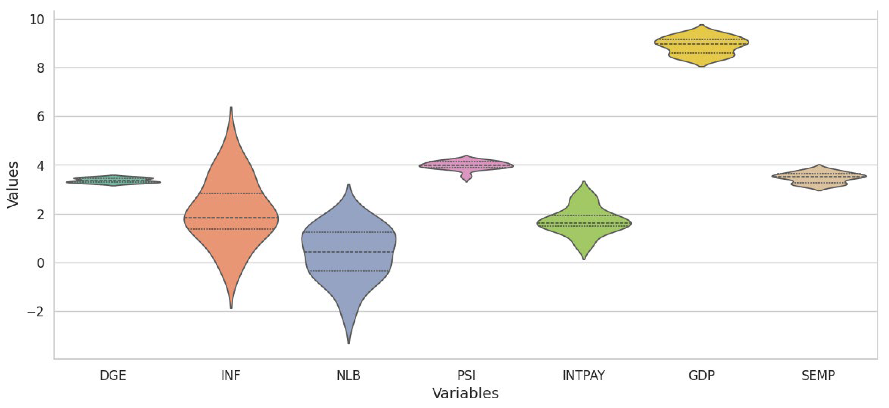
The violin plots in Figure 3 characterize the distribution, density, and central tendency of the variables. The width of each violin reflects the density of data values. The solid line represents the median, while the dashed lines indicate the interquartile range of each distribution. The DGE plot is symmetric, with low variability and stable values. The narrow tail confirms a consistent informal sector. The INF plot is broad, reflecting periods of volatility corresponding to economic transitions. NLB plot tapering reflects lower density at the extremes. The PSI plot is sharply peaked, indicating low variability and political stability. The slight asymmetry points to periods of instability. The INTPAY plot shows high density at lower values, signifying that interest payments have declined. This shape suggests the idea that fiscal sustainability has improved. The GDP plot has a uniform density, indicating limited variability. The SEMP plot has its density concentrated toward lower values, indicating a decline in self-employment.
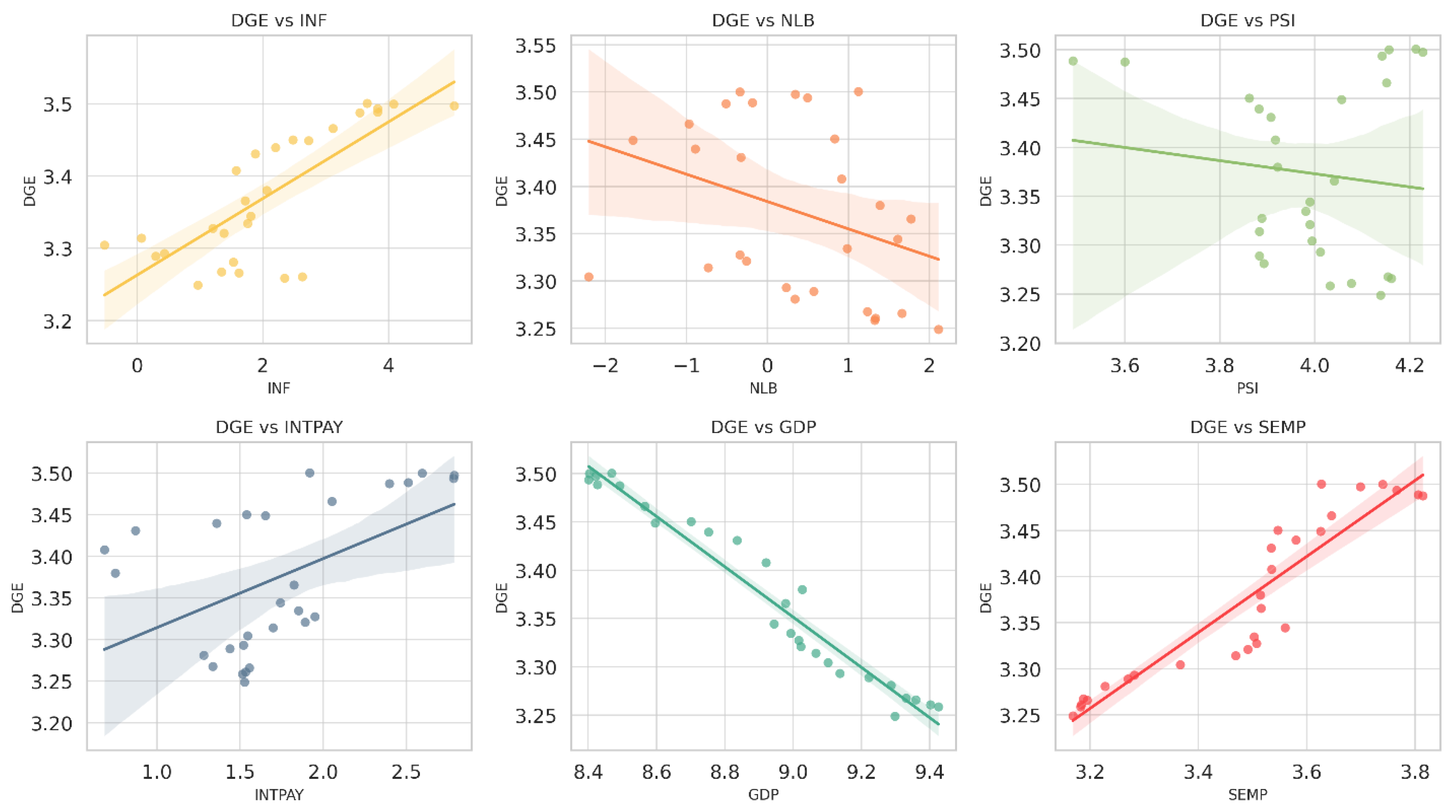
Figure 4 illustrates the relationship between DGE and its determinants. INF, INTPAY, and SEMP are positively associated with DGE, suggesting that higher values of these indicators coincide with greater participation in the shadow economy. GDP and NLB show negative relationships with DGE, implying that stronger economic performance and reduced fiscal pressure tend to diminish shadow economic activity.
PSI has a weak negative link with DGE, which indicates that government institutions may have a limited direct impact on informal economic activities.
These preliminary relationships suggest that Romania’s informal economy is strongly connected to the country’s macroeconomic resilience and institutional stability. Variables such as inflation, fiscal balance, and governance quality represent not only economic indicators but also sustainability dimensions. They reflect SDG 8—Decent Work and Economic Growth—through employment and productivity, and SDG 16—Peace, Justice and Strong Institutions—through institutional credibility. Understanding these linkages is very important for designing sustainable formalization policies that stabilize fiscal revenues and promote inclusive growth.
The Augmented Dickey–Fuller (ADF) method by Dickey and Fuller [69] is used to test data stationarity. The probabilities are shown in parentheses in Table 3. From Table 3, it follows that all variables have an order of integration of one. The results of the ADF test show that only PSI is stationary in level; the rest of the variables become stationary after the first differentiation, thus being first-order integrated (I (1)). Verifying stationarity is very important from a methodological and practical point of view because the ARDL model works with integrated mixed series I (0) and I (1), but assumes the absence of second-order integration (I (2)) [70,71].
According to Table 4, all five criteria suggest that a lag length of 2 is the most favorable selection for the ARDL model. In Table 4, “*” indicates the lag order selected by the criterion. LR represents the sequential modified LR test statistic (each test at 5% level), FPE means Final Prediction Error, AIC is the Akaike Information Criterion, SC means Schwarz information criterion, and HQ is the Hannan–Quinn information criterion. This convergence between the criteria suggests a high level of robustness in determining the length of lags, since, in small or medium samples, the criteria can sometimes produce divergent results. The choice of two lags is also economically coherent: in emerging economies, adjustments to macroeconomic shocks—such as inflation variations, fiscal changes, and institutional changes—rarely propagate instantaneously, but require several periods to be reflected in the transient variables [72,73]. Therefore, the selection of lag 2 confirms both the statistical foundation and the logical connection to Romania’s economic dynamics.
The first step before estimating an ARDL model is to conduct a cointegration analysis using the bounds testing approach. This test aims to either reject or confirm the null hypothesis, which states that there is no cointegration among the variables. The chosen model is ARDL (2,2,1,2,2,2,1). Table 5 reveals that the calculated F-statistic is 5.76, surpassing the upper critical bound for I (1), signifying cointegration among the variables.
We observe that the F-statistic value exceeds the critical upper limits at the thresholds of 1%, 5%, and 10%. Thus, the null hypothesis of the absence of cointegration is rejected, which confirms the existence of a long-term equilibrium relationship between the analyzed variables. Therefore, these results, together with the results in Table 3, fully justify the use of the ARDL model, considering that the variables are integrated I (0) and I (1) and there is a cointegration vector. Moreover, the approach is consistent with sustainability-oriented analyses, as it captures both the short-term shocks and long-term equilibrium adjustments that characterize adaptive economic systems. This is particularly relevant for Romania’s transition economy, where structural reforms and EU convergence create dynamic feedback between fiscal balance, institutional quality, and informal activities.
The estimated long-term coefficients are presented in Table 6. A 1% increase in INF leads to a 0.03% long-term increase in DGE. The size of the informal economy becomes higher when INF increases. Consumers’ purchasing power is diminished by INF while the operational expenses of businesses increase. Then, companies may evade taxes or underreport earnings to preserve profit margins. The informal sector becomes an attractive alternative due to lower compliance costs and fewer regulatory obligations. Informal activities can act as a buffer against economic uncertainty, characterized by monetary policy changes, economic reforms, and external shocks. All these factors cause fluctuations in INF. During times of high INF, workers may prefer informal employment with negotiable wages. It follows that monetary stability is important to reduce informality. Central banks play an essential role by having permanent inflation control, which assists in formalizing the economy. A 1% increase in NLB corresponds to a 0.02% long-term decrease in DGE. This implies that a decline in the formal sector is linked to fiscal restraint and better government finances. A higher NLB reflects sound fiscal management and that a government can finance expenditures without excessive debt. Efficient fiscal policies that produce budget surpluses or lower deficits have the potential to improve public trust in institutions. People are more inclined to observe tax laws when they believe that the government is financially responsible. Business support initiatives and infrastructure development can be financed from fiscal surplus. Healthy fiscal situations in governments can lower taxes, making the formal sector more appealing. A 1-point improvement in the PSI (on a 0–100 scale) reduces DGE by 0.12%. The size of the informal sector is influenced by political stability. The inverse relationship implies that the prevalence of DGE declines with political stability. Political instability raises economic risks by discouraging foreign investments and encouraging informal transactions. Companies may choose to work in the informal sector to reduce the risks associated with policy uncertainty. This relationship is relevant for Romania, which has seen political unrest in recent decades. Better governance, robust institutional quality, and a solid justice system reduce the likelihood of corruption and informal activity. Therefore, better political stability would reduce informality in Romania.
A 1% increase in INTPAY leads to a 0.07% long-term decrease in DGE. Higher government interest obligations are linked with a reduction in informal activity. This outcome might seem counterintuitive, but it reflects the fiscal discipline imposed by debt servicing requirements. In the long run, the negative effect of INTPAY is consistent with economic theory and the literature on fiscal consolidation. The high interest burden forces the state to adopt structural measures to increase collection efficiency, reduce evasion, and modernize tax administration. In Romania, this process was visible with the digitalization of the National Agency for Fiscal Administration (SAF-T, e-Invoice, Virtual Private Space) [74,75,76] and the consolidation of the fiscal framework after EU accession. These measures, together with the pressure to align with European fiscal rules, gradually reduced the space for informal activities and strengthened voluntary compliance, which explains the negative trend in the long run [77,78,79]. Authorities must be forced to increase tax collection to guarantee sufficient revenue when a significant share of government revenue is used for interest payments. This can mean better auditing practices and more rigorous application of tax laws. Fiscal credibility should be maintained, as is expected of an EU member, leading to the formalization of the economy. Debt management and fiscal discipline indirectly curb informality. The most significant factor influencing DGE is GDP. A 1% increase in GDP leads to a 0.29% reduction in DGE. When GDP increases, formalization yields higher revenue; therefore, more businesses are drawn to the formal sector. Higher income, better job prospects in the formal sector, and higher living standards are the results of economic growth. In a prosperous economy, the opportunity cost of informality increases and institutional quality improves. Companies outside the formal sector lose access to credit, contracts, and public goods. Due to higher productivity, the benefits of formality outweigh the costs.
The shift from informality to formality in Romania can be quickened by FDI, EU integration, and structural reforms. This result indicates that measures to increase economic development should be a priority.
A 1% increase in SEMP reduces DGE by 0.18%, which may seem unexpected if self-employment is viewed as a proxy for informal work. However, Romania has undergone major structural changes in the composition of self-employment over the past decade. The decline of agricultural subsistence work and the rapid growth of registered freelancers, individual/family enterprises, and micro-enterprises in urban and professional sectors indicate a shift from informal to formal self-employment. This transformation has been supported by simplified registration procedures, digitalized reporting, and several legislative initiatives stimulating entrepreneurship and innovation [75,80]. Consequently, higher self-employment is associated with greater formal sector engagement, better compliance incentives, and reduced reliance on informal activities [81]. The negative long-run coefficient is therefore consistent with Romania’s gradual structural shift toward formalized freelance and entrepreneurial activity.
The long-run results confirm that sustainable development requires both macroeconomic stability and institutional quality. Inflation control, fiscal responsibility, and effective governance are mutually reinforcing components of a sustainable economic system. Higher GDP per capita and self-employment contribute to inclusive growth when supported by transparent institutions. These findings align with the concept of economic sustainability, where fiscal discipline, productivity, and institutional trust reduce the incentives for informal activity. Consequently, formalization policies should not focus solely on enforcement but also on strengthening the enabling conditions for formal entrepreneurship, innovation, and social protection—the core of SDG 8 and SDG 16.
Table 7 reports the short-run estimated ARDL model. The R-squared (0.93) and Durbin–Watson statistics (2.55) indicate a well-fitted model with no autocorrelation issues. The positive coefficient of the lagged dependent variable indicates strong persistence in the informal sector. 70% of past changes in DGE persist in the current period. This represents the inertia associated with informal activities. It implies that companies continue to operate informally if institutional and economic conditions do not change. In Romania, the informal sector does not adapt immediately to policy changes.
A 1% increase in INF leads to a 0.011% increase in DGE in the same period. Businesses move to the informal sector to avoid higher taxes and wage adjustments, which has an immediate impact. This effect reverses in the subsequent period. This could reflect reactive behavior if the INF becomes stable or if economic agents adapt to inflationary pressures. In Romania, inflationary pressures have been related to external shocks or economic reforms. Reducing the short-term volatility of the informal sector through inflation control can lead to an improvement in formal activities.
A 1% improvement in NLB leads to a 0.0144% reduction in DGE in the short run. This prompt reaction implies that financial restraint increases trust in formal institutions and supports the transition of companies from the informal to the formal sectors. Improvements in fiscal performance mean lower deficits, which creates macroeconomic stability and a decrease in economic risks. Governments lower tax rates and make investments in public services that encourage involvement in the public sector.
A 1-point increase in PSI results in a 0.048% decrease in DGE. A stable political climate deters informal activities. The positive coefficient for lagged PSI suggests that the effect partially reverses in the following period, likely due to the changes in expectations. In Romania, political changes can cause economic disruptions.
A 1% rise in INTPAY leads to a 0.0397% immediate increase in DGE, with a further 0.0212% increase in the following period. Rising INTPAY reflects higher borrowing costs. The increase in interest payments reduces fiscal space and heightens uncertainty about future tax measures. This creates short-term financial pressure on firms, especially small businesses, which may respond by temporarily shifting part of their activity into the informal sector as a coping mechanism. So, in the short term, the positive coefficient associated with INTPAY does not reflect a favorable economic effect on informality, but a behavioral reaction of firms and households to the budgetary pressure generated by the increase in the cost of public debt [11,82,83]. When the state allocates an increasing share of revenues to interest payments, fiscal space is reduced, which often leads to rapid adjustments such as tax increases, increased controls, or postponement of public spending. In Romania, such pressures were visible in the period of 2009–2012 and after 2021, when the increase in the cost of debt coincided with additional fiscal measures [84,85,86]. In such contexts, some small firms and self-employed workers may temporarily resort to undeclared activities as a mechanism for adapting to fiscal uncertainty and deteriorating economic conditions, which translates into a positive coefficient in the short term.
In the short term, DGE is positively impacted by current GDP, likely as a result of a higher demand for informal labor. After one period, economic growth results in a 0.31% reduction in DGE. Both the formal and informal economies are first stimulated by economic growth; formal economies are encouraged later by longer-term gains in income and institutional development.
Short-run innovations in SEMP do not exert a statistically meaningful impact on DGE. This result is expected, given that self-employment in Romania is structurally persistent and does not fluctuate rapidly in response to short-term economic shocks. Most changes in the composition of self-employment occur gradually—through shifts between agricultural, professional, and service sectors—rather than through abrupt quarterly or annual adjustments. Therefore, the insignificant short-run coefficient reflects the slow-moving nature of self-employment dynamics, which limits its relevance in explaining short-term variations in informal output.
ECT measures the speed of adjustment back to the long-run equilibrium after a short-term shock. About 79% of any deviation from the long-run equilibrium is corrected within one year. Such a quick speed points to the efficient underlying mechanisms that stabilize the informal sector.
The short-run responses reveal the adaptive behavior of the informal economy to macroeconomic disturbances. Inflationary shocks, fiscal pressures, and political instability immediately affect informal activity, highlighting the system’s sensitivity to policy shifts. However, the ECT ( 0.79) indicates that almost 80% of these disturbances are corrected within a year, suggesting a high degree of resilience and adaptability. It reflects a fast convergence process. Such a high adjustment speed suggests that Romania’s informal economy responds quite fast to macroeconomic and institutional signals. Temporary shocks in inflation, fiscal balance, governance, or economic activity do not persist but are quickly absorbed by structural mechanisms that restore long-run equilibrium. This result is in line with the findings of Horodnic et al. [5] who argue that informal economic activity in Romania is sensitive to changes in governance quality and fiscal pressures, and that it adapts quickly to changes in institutional incentives.
Table 8 presents the diagnostic and stability tests applied to the ARDL model. All results are statistically insignificant (p-value > 0.05), which means that the null hypotheses are not rejected. Thus, the Serial test confirms the absence of autocorrelation in the residuals, which indicates the independence of the errors. The ARCH test shows that there is no conditional heteroscedasticity, so the error variance is constant. The Jarque–Bera test confirms the normality of the residuals, a sign that the error distribution is appropriate. The Ramsey RESET test indicates the correct specification of the model, without major functional omissions. Therefore, the estimated ARDL model is robust, stable, and correctly specified, fulfilling the main regression assumptions.
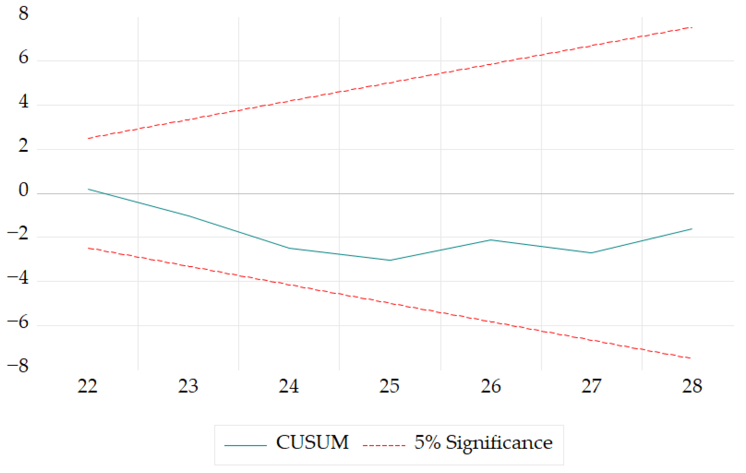
The model’s stability is evaluated using the CUSUM and CUSUM of Squares tests, and the findings are illustrated in Figure 5 and Figure 6. Both tests indicate that the model parameters remain stable, as shown by their trajectories staying within the 5% significance level marked by a red dashed line. Additional robustness checks using CCR, FMOLS, and DOLS are reported in Table A1 (Appendix A), confirming the consistency of the long-run estimates.

5. Discussion

This section discusses how the research questions formulated earlier were addressed through empirical analysis.
RQ1 regards how DGE was affected by macroeconomic factors: INF, GDP, and INTPAY. Both in the short and long run, INF has a positive influence on DGE. Inflationary pressures drive businesses toward informality as a means to cut costs. This finding aligns with the literature, such as Schneider and Enste [11], who emphasize INF’s role in increasing compliance costs and fostering informality. GDP showed a negative relationship with DGE. In line with Loayza [87], economic growth encourages participation in the formal sector by increasing returns to formality. INTPAY has mixed effects. Higher INTPAY increased informality in the short run due to fiscal pressures. In the long run, INTPAY was associated with reduced DGE, reflecting improved fiscal discipline.
RQ2 focused on the role of institutional factors, particularly PSI and NLB. PSI reduced DGE, indicating the importance of stable political environments in promoting formal economic activities, also emphasized by Kaufmann and Kraay [15]. NLB had a negative association with DGE. A better fiscal balance improved confidence in formal institutions, reducing the incentive for informal activities. The same aspect is remarked by Torgler and Schneider [20], who argue that credible fiscal policies enhance institutional trust, thereby encouraging formalization.
RQ3 explored whether SEMP contributes to the reduction in DGE. The ARDL analysis found a negative relationship between SEMP and DGE. This counterintuitive result suggests that in Romania, SEMP increasingly represents formal entrepreneurial activities rather than informal subsistence work. This result agrees with Williams and Round [23], who argue that formal entrepreneurship, supported by institutional frameworks and access to credit reduces informality.
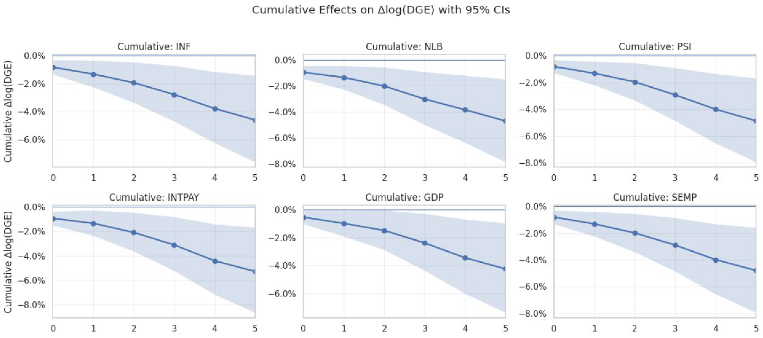
In addition to the statistical relationships resulting from the application of the ARDL model, it is important to understand the dynamic behavior of the informal economy in response to public policy or macroeconomic shocks. Thus, we estimated the Local Projection impulse responses for each variable. The purpose of this analysis was to investigate their effects over a five-year horizon. As can be seen in Figure 6 and Figure 7, the dynamic responses and cumulative effects offer a much more complex perspective on the mechanisms that form regarding the temporal persistence, but also the adjustment of informal production in Romania.
Figure 6 projects the annual short-term effect of a one-unit shock in each exogenous variable on the logarithmic change in the informal economy. We observe that for all variables, a shock causes a decrease in the DGE in the following years. The maximum magnitude is around 1–1.5%, followed by an attenuation. Regarding INF, we observe that it produces a negative short-term response. This means that inflation initially causes an increase in informality, as we observed from the ARDL Model, but the effect gradually dissipates. GDP and PSI confirm that economic growth and political stability reduce informality. INTPAY shows a transitory effect. Increasing interest payments amplifies informality in the short term, but the effect diminishes after 3–4 years. SEMP has a modest and temporarily negative effect.
Figure 8 shows the total cumulative effect over the 5-year horizon, i.e., the duration impact of a shock. We note that all curves are negative and decreasing. This confirms that, in the long run, macroeconomic and institutional factors reduce informality. The largest observed contribution is made by GDP, PSI and NLB. Therefore, economic growth, political stability and fiscal balance have structural effects on the formalization of the economy.
In conclusion, the results of our study provide consistent directions and answers to the four stability research questions. Regarding RQ1, we observe that inflation and interest payments stimulate informal activity in the short term. On the other hand, GDP per capita shows a persistent formalization effect. This confirms the role of macroeconomic stability in supporting inclusive growth. From the perspective of RQ2, institutional quality, described by political stability and fiscal balance, is a decisive factor in reducing informality. This happens because it increases trust in formal structures. Moreover, it strengthens incentives for compliance. Regarding RQ3, self-employment no longer appears as a factor of informality. On the other hand, self-employment represents more of a transition towards formal entrepreneurship and labor market modernization. Last but not least, RQ4 is addressed by the high adjustment coefficient in the ARDL error correction term ( 0.79), but also by the dynamics of the Local Projection. Both highlight the fact that Romania’s informal economy moves relatively quickly, within two to three years, towards long-term equilibrium following macroeconomic shocks. Therefore, these results reinforce the need for sustainable formalization. This, in turn, requires a stable macroeconomic environment, credible institutions, but also policies to support entrepreneurship and fiscal transparency. From this point of view, Romania’s direction towards reducing informality aligns with the broader Sustainable Development Goals (SDGs): SDG8—decent work and economic growth, as well as SDG16—peace, justice and strong institutions. For example, by strengthening institutions and improving fiscal discipline, informal activities can be reduced. This direction is consistent with SDG16 because both political stability and governance quality improve voluntary compliance and reduce undeclared activities. Also, introducing macroeconomic policies, reducing fiscal pressure, and stimulating productivity to avoid informal activities are in line with SDG8. This aspect is reinforced by the institutional and fiscal reforms implemented in Romania, such as the digitalization of tax administration through e-Invoice, SAF-T, or Virtual Private Space.

6. Conclusions

The empirical analysis of Romania’s informal economy reveals several aspects. INF exerts a positive influence on DFE in both the short and long term. Price instability drives businesses to operate informally to overcome inflation-induced costs. NLB exhibits a negative relationship with DGE. Prudent fiscal management stimulates confidence in formal institutions, thereby diminishing the inclination for informal economic activities. PSI contributes to a reduction in DGE by creating an environment that encourages formal economic activity. The presence of short-term fluctuations implies that continuous political stability is essential to achieve lasting formalization. INTPAY has mixed effects; higher INTPAY correlates with a rise in DGE in the short run, while long-term effects reflect a better fiscal discipline. GDP has a role in curbing informality. Economic expansion increases the advantages of formalization, raises living standards, and deters participation in the informal sector. SEMP has a negative correlation with DGE over the long term; entrepreneurship bolsters formal sector involvement. The error correction mechanism indicates a swift adjustment rate of 79%, signifying that Romania’s informal economy is responsive to policy interventions and macroeconomic fluctuations.
Although the empirical results have been validated as robust and supported by diagnostic tests and additional checks, it is important to acknowledge the limitations of our study. First, the informality indicator (DGE) is a model derived from a general equilibrium model and does not capture a directly observed value. Although this aspect may introduce some uncertainty in the magnitude of the coefficients, the specialized literature uses DGE analysis in various ways. Although the ARDL framework partially mitigates the endogeneity problem through dynamic structure and the use of the error correction mechanism, the existence of inverse relationships cannot be completely ruled out. For example, GDP per capita, the fiscal balance, or political stability can influence informality, but can also be influenced by it. In this sense, the CCR, FMOLS, and DOLS estimates confirm the robustness of the coefficients in the long run. Another limitation could be generated by the fact that the model, although it includes the main macroeconomic, fiscal, and institutional determinants of informality, other factors could also be relevant. Future research directions could include factors such as labor market segmentation, degree of digitalization, and sectoral informality.
Several policy recommendations are proposed to mitigate informality in Romania. First, inflation-targeting measures diminish the short-term volatility that causes informal activities. Second, balanced budgets and reducing public debt strengthen institutional credibility and promote participation in the formal sector. Third, reinforcing political institutions and stable governance alleviates uncertainty and attracts formal investments. Fourth, public debt management, which lowers interest obligations mitigates immediate pressures that drive economic agents toward informality. Fifth, economic growth driven by structural reforms, innovation, and infrastructure development facilitates formalization. Sixth, supporting entrepreneurship can encourage formal SEMP. The transition from informal to formal activity can be encouraged by improving tax administration and reforming tax policies to reduce the fiscal burden

Author Contributions

Conceptualization, I.G. and I.N.; methodology, I.G. and I.N.; software, I.G. and I.N.; validation, I.G., I.N., N.C. and J.K.; formal analysis, I.G.; investigation, I.G. and I.N.; resources, I.N. and J.K.; data curation, I.G., I.N., N.C. and J.K.; writing—original draft preparation, I.G. and I.N.; writing—review and editing, I.G., I.N., N.C. and J.K.; visualization, I.G., I.N., N.C. and J.K.; supervision, I.G. and I.N.; project administration, I.N.; funding acquisition, I.N. All authors have read and agreed to the published version of the manuscript.

Funding

This work was funded by the EU’s NextGenerationEU instrument through the National Recovery and Resilience Plan of Romania—Pillar III-C9-I8, managed by the Ministry of Research, Innovation and Digitization, within the project entitled “Place-based Economic Policy in EU’s Periphery—fundamental research in collaborative development and local resilience. Projections for Romania and Moldova (PEPER)”, contract No. 760045/23.05.2023, code CF 275/30.11.2022.

Institutional Review Board Statement

Not applicable.

Informed Consent Statement

Not applicable.

Data Availability Statement

Data are available upon request.

Conflicts of Interest

The authors declare no conflicts of interest.

Appendix A. Robustness Checks Using CCR, FMOLS, and DOLS

The long-run coefficients obtained from CCR, FMOLS, and DOLS, reported in Table A1, are generally consistent with the ARDL results. For all three estimators, INF is stable, positive, and statistically significant. This convergence is important, since the INF–informality relationship is known to be sensitive to endogeneity and dynamic feedback effects, according to Schneider and Enste (2000) [11]. The fact that INF has about the same coefficient for CCR, FMOLS, and DOLS indicates that the effect of INF is structural. INTPAY has a negative and significant coefficient, with similar values. It follows that high-interest payment burdens, representing fiscal pressures, reduce informal activity [20,87]. GDP has the strongest and most stable effect, about the same size as the ARDL coefficient. It implies that economic development reduces informal activities, in agreement with the literature stating that institutional capacity is strengthened [88]. PSI, NLB, and SEMP retain their expected signs, but they are not statistically significant. This result is common when applying conservative long-run variance corrections in small-sample annual data. The ARDL findings are not contradicted. PSI, NLB, and SEMP influence informal activity by a short-run adjustment mechanism, captured by the ARDL-ECM [58]. Their weak statistical significance in CCR, FMOLS, and DOLS reflect methodological differences rather than theoretical inconsistency.
Table A1. Robustness results using CCR, FMOLS, and DOLS estimators.
VariableCCR
Coefficient
CCR
t-Statistic
FMOLS
Coefficient
FMOLS
t-Statistic
DOLS
Coefficient
DOLS
t-Statistic
INF0.014023 ***5.78210.013830 ***7.44480.013568 ***6.6748
NLB 0.001292 0.5875 0.000861 0.5308 0.000443 0.2585
PSI 0.003473 0.2849 0.004644 0.4879 0.007482 0.7141
INTPAY 0.039803 *** 11.407 0.039751 *** 12.3239 0.039030 *** 11.0481
GDP 0.253100 *** 12.4026 0.256734 *** 14.1033 0.253516 *** 13.8757
SEMP0.0087060.30190.0054410.16980.0108040.3927
C5.652873 ***18.5255.705108 ***21.4765.664736 ***20.478
*** indicates the significance of variables at 1% level.
The model diagnostics in Table A2 reinforce the stability of the results. The R-squared values are close to 0.99, the standard errors of regression are similar, and the long-run variance value is small. This points to a strong cointegration relation.
Table A2. Model diagnostics for CCR, FMOLS, and DOLS estimators.
StatisticCCRFMOLSDOLS
R-squared0.98970.98970.9906
Adjusted R-squared0.98660.98660.9879
S.E. of regression0.0102290.0102130.009922
Long-run variance 4.31 × 10 5 4.31 × 10 5 5.28 × 10 5

References

  1. Ameer, W.; Sohag, K.; Zhan, Q.; Shah, S.H.; Yongjia, Z. Do Financial Development and Institutional Quality Impede or Stimulate the Shadow Economy? A Comparative Analysis of Developed and Developing Countries. Humanit. Soc. Sci. Commun. 2025, 12, 17. [Google Scholar] [CrossRef]
  2. Mara, E.R.; Maran, R. Are Fiscal Rules Efficient on Public Debt Restraint in the Presence of Shadow Economy? Financ. Res. Lett. 2024, 64, 105495. [Google Scholar] [CrossRef]
  3. Horodnic, I.A.; Williams, C.C.; Apetrei, A.; Mațcu, M.; Horodnic, A.V. Services Purchase from the Informal Economy Using Digital Platforms. Serv. Ind. J. 2023, 43, 854–874. [Google Scholar] [CrossRef]
  4. Ivan, A.-D.; Davidescu, A.A.; Agafiţei, M.-D.; Geambaşu, M.C. Applying Machine Learning Techniques to Estimate the Size of the Romanian Shadow Economy. Proc. Int. Conf. Bus. Excell. 2025, 19, 2525–2541. [Google Scholar] [CrossRef]
  5. Horodnic, I.A.; Williams, C.C.; Țugulea, O.; Stoian Bobâlcă, I.C. Exploring the Demand-Side of the Informal Economy during the COVID-19 Restrictions: Lessons from Iași, Romania. Sustainability 2022, 14, 7228. [Google Scholar] [CrossRef]
  6. Ackrill, R.; Igudia, E. Analysing the Informal Economy: Data Challenges, Research Design, and Research Transparency. Rev. Dev. Econ. 2024, 28, 1971–1993. [Google Scholar] [CrossRef]
  7. Medina, L.; Schneider, F. Shadow Economies Around the World: What Did We Learn over the Last 20 Years? IMF Working Papers; International Monetary Fund: Washington, DC, USA, 2018; Volume 18, p. 1. [Google Scholar] [CrossRef]
  8. Buehn, A.; Schneider, F. Shadow Economies around the World: Novel Insights, Accepted Knowledge, and New Estimates. Int. Tax. Public Financ. 2012, 19, 139–171. [Google Scholar] [CrossRef]
  9. Sultana, N.; Rahman, M.M.; Murad, S.M.W. Asymmetric Role of the Informal Sector on Economic Growth: Empirical Investigation on a Developing Country. Struct. Change Econ. Dyn. 2024, 69, 96–107. [Google Scholar] [CrossRef]
  10. Taheri, E.; Katircioğlu, S.; Tecel, A. Gender Differences in the Impact of the Informal Economy on the Labor Market: Evidence From Middle Eastern Countries. Eval. Rev. 2024, 48, 865–892. [Google Scholar] [CrossRef] [PubMed]
  11. Schneider, F.; Enste, D.H. Shadow Economies: Size, Causes, and Consequences. J. Econ. Lit. 2000, 38, 77–114. [Google Scholar] [CrossRef]
  12. Ștefoni, S.E.; Brașoveanu, I.V.; Butu, I. Social Aspects of the Informal Economy: Evidence from EU Countries. Theor. Appl. Econ. 2024, 31, 197–210. [Google Scholar]
  13. Gillanders, R.; Parviainen, S. Corruption and the Shadow Economy at the Regional Level. Rev. Dev. Econ. 2018, 22, 1729–1743. [Google Scholar] [CrossRef]
  14. Alm, J.; Embaye, A. Using Dynamic Panel Methods to Estimate Shadow Economies Around the World, 1984–2006. Public Financ. Rev. 2013, 41, 510–543. [Google Scholar] [CrossRef]
  15. Kaufmann, D.; Kraay, A. Growth without Governance. Economía 2002, 3, 169–229. [Google Scholar] [CrossRef]
  16. Elbahnasawy, N.G. Can E-Government Limit the Scope of the Informal Economy? World Dev. 2021, 139, 105341. [Google Scholar] [CrossRef]
  17. Nedić, V.; Despotović, D.; Cvetanović, S.; Djukić, T.; Petrović, D. Institutional Reforms for Economic Growth in the Western Balkan Countries. J. Policy Model. 2020, 42, 933–952. [Google Scholar] [CrossRef]
  18. International Monetary Fund; Dabla-Norris, E.; Koeda, J. Informality and Macroeconomic Fluctuations. In IMF Research Bulletin, December 2008; IMF Research Bulletin; International Monetary Fund: Washington, DC, USA, 2008; Volume 8, p. 1. [Google Scholar] [CrossRef]
  19. Huynh, C.M.; Nguyen, T.L. Fiscal Policy and Shadow Economy in Asian Developing Countries: Does Corruption Matter? Empir. Econ. 2020, 59, 1745–1761. [Google Scholar] [CrossRef]
  20. Torgler, B.; Schneider, F.G. Shadow Economy, Tax Morale, Governance and Institutional Quality: A Panel Analysis. SSRN J. 2007. [Google Scholar] [CrossRef]
  21. Goel, R.; Saunoris, J. Forms of Government Decentralization and Institutional Quality: Evidence from a Large Sample of Nations. In Central and Local. Government Relations in Asia; Yoshino, N., Morgan, P.J., Eds.; Edward Elgar Publishing: Cheltenham, UK, 2017; pp. 395–420. [Google Scholar]
  22. Oviedo, A.M.; Thomas, M.; Karakurum-Ozdemir, K. Economic Informality: Causes, Costs, and Policies—A Literature Survey; World Bank Working Paper; 2009. [Google Scholar] [CrossRef]
  23. Williams, C.C.; Round, J. Evaluating Informal Entrepreneurs’ Motives: Evidence from Moscow. Int. J. Entrep. Behav. Res. 2009, 15, 94–107. [Google Scholar] [CrossRef]
  24. Nguyen, C.P.; Schinckus, C.; Nguyen, Q.B.; Le Tran, D.T. Digitalization and Informal Economy: A Global Evidence of Internet Usage. J. Ind. Bus. Econ. 2024, 51, 1–37. [Google Scholar] [CrossRef]
  25. Frost, J.; Kamin, S.; Aguilar, A.; Guerra, R.; Tombini, A. Digital Payments, Informality and Economic Growth 2024. Available online: https://www.bis.org/publ/work1196.pdf (accessed on 24 October 2025).
  26. Krichewsky-Wegener, L. Digital Transformation in the Informal Economy: Opportunities and Challenges for Technical and Vocational Education and Training in Development Cooperation. Available online: https://www.govet.international/en/129448.php (accessed on 24 October 2025).
  27. Chacaltana Janampa, J.; Mattos, F.B.D.; García, J.M.; International Labour Organization. Employment Policy Department. In New Technologies, e-Government and Informality; ILO: Geneva, Switzerland, 2024; ISBN 978-92-2-040568-0. [Google Scholar]
  28. Sarkar, O.T.; Hasan, M.A.; Saha, S.K. Resilience in the Informal Economy amidst the COVID-19 Crisis: The Experience of Street Vendors in Dhaka, Bangladesh. Urban Plan. Transp. Res. 2025, 13, 2502001. [Google Scholar] [CrossRef]
  29. Fridayani, H.D.; Chiang, L.-C.; Atmojo, M.E.; Tai, K.-T. Empowering Resilience: How Digital Tools and Environmental Practices Can Foster Growth in the Informal Business Sector. IOP Conf. Ser. Earth Environ. Sci. 2025, 1475, 012001. [Google Scholar] [CrossRef]
  30. Yazdanie, M.; Frimpong, P.B.; Dramani, J.B.; Orehounig, K. The Impacts of the Informal Economy, Climate Migration, and Rising Temperatures on Energy System Planning. Energy Rep. 2024, 11, 165–178. [Google Scholar] [CrossRef]
  31. Cartwright, E.; Igudia, E. The Case for Mixed Methods Research: Embracing Qualitative Research to Understand the (Informal) Economy. Rev. Dev. Econ. 2024, 28, 1947–1970. [Google Scholar] [CrossRef]
  32. Abid, M.; Sekrafi, H.; Gheraia, Z.; Abdelli, H. Regulating the Unobservable: The Impact of the Environmental Regulation on Informal Economy and Pollution. Energy Environ. 2024, 35, 3463–3482. [Google Scholar] [CrossRef]
  33. Nica, I.; Georgescu, I.; Delcea, C.; Chiriță, N. Toward Sustainable Development: Assessing the Effects of Financial Contagion on Human Well-Being in Romania. Risks 2023, 11, 204. [Google Scholar] [CrossRef]
  34. Elgin, C.; Oztunali, O. Institutions, Informal Economy, and Economic Development. Emerg. Mark. Financ. Trade 2014, 50, 145–162. [Google Scholar] [CrossRef]
  35. Khuong, N.V.; Shabbir, M.S.; Sial, M.S.; Khanh, T.H.T. Does Informal Economy Impede Economic Growth? Evidence from an Emerging Economy. J. Sustain. Financ. Invest. 2021, 11, 103–122. [Google Scholar] [CrossRef]
  36. Nouhessèwa Hounyonou, Q. How Does the Informal Economy Affect SDGs in Developing Countries? Int. J. Sustain. Dev. World Ecol. 2025, 32, 589–617. [Google Scholar] [CrossRef]
  37. Salinas, A.; Ortiz, C. Exploring the Relationship between Productive Structure and the Informal Economy: Evidence from Latin American Countries. JEPP 2024, 13, 306–332. [Google Scholar] [CrossRef]
  38. Lyeonov, S.; Moroz, A.; Dudziuk, I.; Chuluunbaatar, E. Green Rules & Grey Markets: Do Environmental Policies Influence the Informal Economy? Econ. Sociol. 2025, 18, 313–338. [Google Scholar] [CrossRef]
  39. Abdulkadr, A.A.; Asnakew, Y.W.; Sendkie, F.B.; Workineh, E.B.; Asfaw, D.M. Analyzing the Dynamics of Monetary Policy and Economic Growth in Ethiopia: An Autoregressive Distributed Lag (ARDL) Approach. Discov. Sustain. 2024, 5, 90. [Google Scholar] [CrossRef]
  40. Kanayo, O.; Maponya, L.; Semenya, D. Evaluating the Dynamic Effects of Environmental Taxation and Energy Transition on Greenhouse Gas Emissions in South Africa: An Autoregressive Distributed Lag (ARDL) Approach. Sustainability 2025, 17, 5531. [Google Scholar] [CrossRef]
  41. Gwaindepi, A. Taxation in the Context of High Informality: Conceptual Challenges and Evidence from Sub-Saharan Africa. Rev. Dev. Econ. 2025, 29, 1228–1249. [Google Scholar] [CrossRef]
  42. Dell’Anno, R. Integrating National Accounting and Macroeconomic Approaches to Estimate the Underground, Informal, and Illegal Economy in European Countries. Int. Tax. Public Financ. 2025, 32, 526–565. [Google Scholar] [CrossRef]
  43. Wiafe, P.A.; Armah, M.; Ahiakpor, F.; Tuffour, K.A. The Underground Economy and Tax Evasion in Ghana: Implications for Economic Growth. Cogent Econ. Financ. 2024, 12, 2292918. [Google Scholar] [CrossRef]
  44. Polese, A.; Moisé, G.M.; Tokyzhanova, T.; Aguzzi, T.; Kerikmäe, T.; Sagynbaeva, A.; Sauka, A.; Seliverstova, O. Informality versus Shadow Economy: Reflecting on the First Results of a Manager’s Survey in Kyrgyzstan. Cent. Asian Surv. 2023, 42, 149–170. [Google Scholar] [CrossRef]
  45. Elgin, C.; Kose, A.; Ohnsorge, F.; Yu, S. Understanding Informality. 2021. Available online: https://cepr.org/publications/dp16497 (accessed on 24 October 2025).
  46. World Bank Inflation, Consumer Prices (Annual %) 2025. Available online: https://data.worldbank.org/indicator/FP.CPI.TOTL.ZG (accessed on 20 August 2025).
  47. International Monetary Fund Primary Net Lending/Borrowing (Also Referred as Primary Balance) % of GDP 2025. Available online: https://www.imf.org/external/datamapper/GGXONLB_G01_GDP_PT@FM/ADVEC/FM_EMG/FM_LIDC/ROU (accessed on 20 August 2025).
  48. World Bank Political Stability and Absence of Violence/Terrorism: Percentile Rank 2025. Available online: https://data.worldbank.org/indicator/PV.PER.RNK (accessed on 20 August 2025).
  49. World Bank Interest Payments (% of Revenue) 2025. Available online: https://data.worldbank.org/indicator/GC.XPN.INTP.RV.ZS (accessed on 20 August 2025).
  50. World Bank GDP per Capita (Constant 2015 US$) 2025. Available online: https://data.worldbank.org/indicator/NY.GDP.PCAP.KD (accessed on 20 August 2025).
  51. Jordà, Ò. Estimation and Inference of Impulse Responses by Local Projections. Am. Econ. Rev. 2005, 95, 161–182. [Google Scholar] [CrossRef]
  52. Elgin, C.; Oztunali, O. Shadow Economies around the World: Model Based Estimates 2012. Available online: https://EconPapers.repec.org/RePEc:bou:wpaper:2012/05 (accessed on 15 September 2025).
  53. Ihrig, J.; Moe, K.S. Lurking in the Shadows: The Informal Sector and Government Policy. J. Dev. Econ. 2004, 73, 541–557. [Google Scholar] [CrossRef]
  54. Elgin, C.; Kose, A.; Ohnsorge, F.; Yu, S. Shades of Grey: Measuring the Informal Economy Business Cycles 2019. Available online: https://www.imf.org/-/media/files/conferences/2019/7th-statistics-forum/session-ii-yu.pdf (accessed on 15 September 2025).
  55. Copaciu, M.; Nalban, V.; Bulete, C. REM, 2.0, An Estimated DSGE Model for Romania. In Proceedings of the 11th Dynare Conference, Brussels, Belgium, 28–29 September 2015. [Google Scholar]
  56. Lütkepohl, H.; Xu, F. The Role of the Log Transformation in Forecasting Economic Variables. Empir. Econ. 2012, 42, 619–638. [Google Scholar] [CrossRef]
  57. Lütkepohl, H. New Introduction to Multiple Time Series Analysis; Springer: Berlin/Heidelberg, Germany, 2005; ISBN 978-3-540-40172-8. [Google Scholar]
  58. Pesaran, M.H.; Shin, Y.; Smith, R.J. Bounds Testing Approaches to the Analysis of Level Relationships. J. Appl. Econom. 2001, 16, 289–326. [Google Scholar] [CrossRef]
  59. Pesaran, M.H. An Autoregressive Distributed-Lag Modelling Approach to Cointegration Analysis. In Econometrics and Economic Theory in the 20th Century: The Ragnar Frisch Centennial Symposium; Strøm, S., Ed.; Cambridge University Press: New York, NY, USA, 1998; pp. 371–413. ISBN 978-0-521-63323-9. [Google Scholar]
  60. Xuan, V.N. An ARDL Approach to Investigating the Relationship between FDI, Renewable Energy, Economic Growth, Trade Openness, and CO2 Emissions in Australia. Results Eng. 2025, 27, 105668. [Google Scholar] [CrossRef]
  61. Nkoro, E.; Uko, K. Autoregressive Distributed Lag (ARDL) Cointegration Technique: Application and Interpretation. J. Stat. Econom. Methods 2016, 5, 63–91. [Google Scholar]
  62. Delcea, C.; Nica, I.; Georgescu, I.; Chiriță, N.; Ciurea, C. Integrating Fuzzy MCDM Methods and ARDL Approach for Circular Economy Strategy Analysis in Romania. Mathematics 2024, 12, 2997. [Google Scholar] [CrossRef]
  63. Georgescu, I.; Nica, I.; Delcea, C.; Chiriță, N.; Ionescu, Ș. Assessing Regional Economic Performance in Romania Through Panel ARDL and Panel Quantile Regression Models. Sustainability 2024, 16, 9287. [Google Scholar] [CrossRef]
  64. Park, J.Y. Canonical Cointegrating Regressions. Econometrica 1992, 60, 119. [Google Scholar] [CrossRef]
  65. Phillips, P.C.B.; Hansen, B.E. Statistical Inference in Instrumental Variables Regression with I(1) Processes. Rev. Econ. Stud. 1990, 57, 99. [Google Scholar] [CrossRef]
  66. Stock, J.H.; Watson, M.W. A Simple Estimator of Cointegrating Vectors in Higher Order Integrated Systems. Econometrica 1993, 61, 783. [Google Scholar] [CrossRef]
  67. International Monetary Fund. IMF Research Bulletin, December 2008; IMF Research Bulletin; International Monetary Fund: Washington, DC, USA, 2008; Volume 9, p. 1. [Google Scholar] [CrossRef]
  68. Huynh, C.M.; Nguyen, T.L. Shadow Economy and Income Inequality: New Empirical Evidence from Asian Developing Countries. J. Asia Pac. Econ. 2020, 25, 175–192. [Google Scholar] [CrossRef]
  69. Dickey, D.A.; Fuller, W.A. Distribution of the Estimators for Autoregressive Time Series with a Unit Root. J. Am. Stat. Assoc. 1979, 74, 427–431. [Google Scholar] [CrossRef]
  70. Ngoc, X.V. Determinants of Open Innovation in United State of America: New Evidence from ARDL Method. Innov. Green. Dev. 2025, 4, 100228. [Google Scholar] [CrossRef]
  71. Nica, I.; Georgescu, I.; Kinnunen, J. Evaluating Renewable Energy’s Role in Mitigating CO2 Emissions: A Case Study of Solar Power in Finland Using the ARDL Approach. Energies 2024, 17, 4152. [Google Scholar] [CrossRef]
  72. Cevik, S.; Miryugin, F. It’s Never Different: Fiscal Policy Shocks and Inflation; IMF Working Papers; International Monetary Fund: Washington, DC, USA, 2023; ISBN 979-8-4002-4287-8. [Google Scholar]
  73. Sungurtekin Hallam, B. Emerging Market Responses to External Shocks: A Cross-Country Analysis. Econ. Model. 2022, 115, 105948. [Google Scholar] [CrossRef]
  74. Deloitte The Digitalization Marathon: Implementing SAF-T in Romania. Available online: https://www.deloitte.com/ro/ro/services/tax/services/maratonul-digitalizarii-implementarea-saf-t-in-romania.html (accessed on 22 November 2025).
  75. European Commission eInvoicing in Romania. Available online: https://ec.europa.eu/digital-building-blocks/sites/spaces/DIGITAL/pages/467108898/eInvoicing+in+Romania (accessed on 22 November 2025).
  76. PricewaterhouseCoopers Romania: Corporate—Tax Administration. Available online: https://taxsummaries.pwc.com/romania/corporate/tax-administration (accessed on 22 October 2025).
  77. OECD. Tax Administration 2025: Comparative Information on OECD and Other Advanced and Emerging Economies; OECD Publishing: Paris, France, 2025; ISBN 978-92-64-55706-2. [Google Scholar]
  78. International Monetary Fund ROMANIA—TECHNICAL ASSISTANCE REPORT ON IMPROVING REVENUES FROM THE RECURRENT PROPERTY TAX 2022. Available online: https://www.imf.org/-/media/Files/Publications/CR/2022/English/1ROUEA2022001.ashx (accessed on 22 October 2025).
  79. Kommission, E. (Ed.) 2023 Country Report Romania; Publications Office of the European Union: Luxembourg, 2023; ISBN 978-92-68-03214-5. Available online: https://data.europa.eu/doi/10.2765/34357 (accessed on 22 October 2025).
  80. Kinnunen, J.; Georgescu, I.; Hosseini, Z.; Androniceanu, A.-M. Dynamic Indexing and Clustering of Government Strategies to Mitigate COVID-19. EBER 2021, 9, 7–20. [Google Scholar] [CrossRef]
  81. Laing, E.; Van Stel, A.; Storey, D.J. Formal and Informal Entrepreneurship: A Cross-Country Policy Perspective. Small Bus. Econ. 2022, 59, 807–826. [Google Scholar] [CrossRef]
  82. Loayza, N.; Serven, L.; Sugawara, N. Informality in Latin America and the Caribbean. World Bank Policy Res. Work. Pap. 2010. [Google Scholar]
  83. Enste, D. The Shadow Economy in Industrial Countries. IZA World Labor 2015. [Google Scholar] [CrossRef]
  84. Williams, C.C.; Horodnic, I.A. Explaining the Informal Economy in Post-Communist Societies: A Study of the Asymmetry Between Formal and Informal Institutions in Romania. In The Informal Economy in Global Perspective; Polese, A., Williams, C.C., Horodnic, I.A., Bejakovic, P., Eds.; Springer International Publishing: Cham, Switzerland, 2017; pp. 117–140. ISBN 978-3-319-40930-6. [Google Scholar]
  85. Asllani, A.; Schneider, F. A Review of the Driving Forces of the Informal Economy and Policy Measures for Mitigation: An Analysis of Six EU Countries. Int. Tax. Public Financ. 2025, 32, 310–344. [Google Scholar] [CrossRef]
  86. Si, C.; Hassan, F.A.; Antohi, V.M.; Ahmad, W.; Fortea, C.; Cristache, N.; Alshammari, F.; Zlati, M.L. Informal Economy and Environmental Degradation in Developing Countries: The Conditioning Role of Institutional Quality. Front. Environ. Sci. 2025, 13, 1645194. [Google Scholar] [CrossRef]
  87. Loayza, N.V. The Economics of the Informal Sector: A Simple Model and Some Empirical Evidence from Latin America. Carnegie-Rochester. Conf. Ser. Public Policy 1996, 45, 129–162. [Google Scholar] [CrossRef]
  88. Williams, C.C.; Schneider, F. Measuring the Global Shadow Economy: The Prevalence of Informal Work and Labour; Edward Elgar Publishing: Cheltenham, UK, 2016. [Google Scholar]
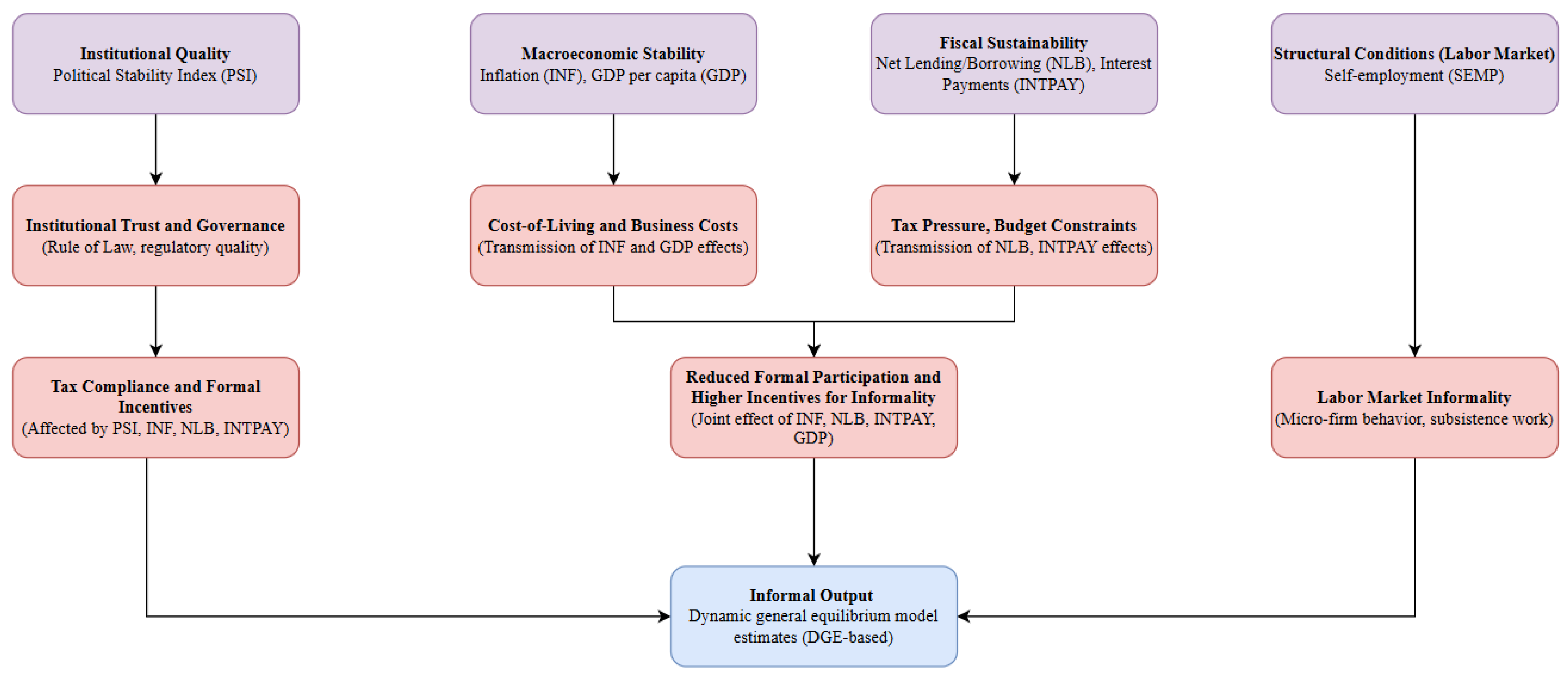
Figure 1. Conceptual framework linking institutional quality, macroeconomic stability, fiscal sustainability, and labor-market conditions to informal output.
Sustainability 17 10920 g001
Figure 2. Time evolution of log-transformed variables for Romania (1995–2023).
Sustainability 17 10920 g002
Figure 3. Violin plots for DGE, INF, NLB, PSI, INTPAY, GDP, SEMP.
Sustainability 17 10920 g003
Figure 4. Scatterplots with fitted lines between DGE and explanatory variables.
Sustainability 17 10920 g004
Figure 5. Stability of ARDL model parameters based on the CUSUM test.
Sustainability 17 10920 g005
Figure 6. Stability of ARDL model parameters based on the CUSUM of Squares test.
Sustainability 17 10920 g006
Figure 7. Dynamic responses of informal output to macroeconomic and institutional shocks. Dynamic responses of the logarithmic change in informal output ( log D G E ) to one-unit shocks in inflation (INF), fiscal balance (NLB), political stability (PSI), interest payments (INTPAY), GDP per capita (GDP), and self-employment (SEMP). Shaded areas represent 95% bootstrap confidence intervals obtained through Local Projections over a 5-year horizon.
Sustainability 17 10920 g007
Figure 8. Cumulative effects of macroeconomic and institutional variables on informal output. Cumulative long-term effects of one-unit shocks in macroeconomic and institutional variables on the logarithmic change in informal output ( log D G E ) , based on Local Projections [51]. The results show the total impact accumulated over a 5-year horizon, with 95% bootstrap confidence intervals.
Sustainability 17 10920 g008
Table 1. Variables specification.
VariableAcronymMeasurement UnitSource
Dynamic general equilibrium model-based (DGE) estimates of informal outputDGE% of official GDPWorld Bank [45]
Inflation, consumer prices, annualINF%World Bank [46]
Primary net lending/borrowing (also referred as primary balance)NLB% of GDPInternational Monetary Fund [47]
Political Stability and Absence of Violence/TerrorismPSI[0, 100]World Bank [48]
Interest payments (% of revenue)INTPAY%World Bank [49]
Gross domestic product per capitaGDPConstant 2015 USDWorld Bank [50]
Self-employment (% of total employment)SEMP%World Bank [45]
Table 2. Summary statistics.
DGEINFNLBPSIINTPAYGDPSEMP
Mean3.373862.0917250.3504453.9872861.7178558.914073.48348
Median3.3549711.8438220.4191433.9918861.6031578.9852573.514817
Maximum3.5005895.0418982.1102134.227612.7879129.4253713.813962
Minimum3.248898−0.520613−2.2072753.4905580.6833528.4015093.168301
Std. Dev.0.0901061.3104091.0828610.1685410.5417860.3379540.20327
Skewness0.133380.207701−0.449477−1.0721220.263207−0.17715−0.185139
Kurtosis1.4722872.6781192.5343454.5035942.8781141.7643631.938325
Jarque–Bera2.8059120.3221941.1957798.0016740.340631.9277161.474971
Probability0.2458690.8512090.5499710.01830.8433990.3814190.478315
Table 3. ADF unit root test results.
VariablesLevelFirst DifferenceOrder of Integration at 5% L.O.S.
T-StatisticsT-Statistics
DGE−0.60 (0.854)−4.05 *** (0.004)I (1)
INF−1.54 (0.497)−6.23 *** (0.000)I (1)
NLB−2.60 (0.103)−6.35 *** (0.000)I (1)
PSI−3.61 ** (0.012)−5.93 *** (0.00))I (0)
INTPAY−2.41 (0.148)−5.39 *** (0.000)I (1)
GDP0.10 (0.960)−4.05 *** (0.004)I (1)
SEMP0.03 (0.954)−4.66 *** (0.001)I (1)
** and *** Indicate the significance of variables at 5% and 1% levels, respectively.
Table 4. VAR lag order selection criteria.
LagLogLLRFPEAICSCHQ
056.43N/A 5.27 × 10 11 3.80 3.46 3.70
1212.78216.48 1.58 × 10 14 12.06 9.35 11.28
2301.1974.80 * 2.04 × 10 15   * 15.09 * 10.01 * 13.62 *
“*” indicates the lag order selected by the criterion.
Table 5. Results of ARDL cointegration bound test.
Test StatisticValueK (Number of Regressors)
F-Statistic5.766
Critical value bounds
SignificanceI (0)I (1)
10%1.992.94
5%2.273.28
1%2.883.99
Table 6. Long-run estimated results of the ARDL (2,2,1,2,2,2,1) model.
VariablesCoefficientT-StatisticsProb.
INF0.034.010.005 ***
NLB 0.02 2.500.040 **
PSI 0.12 2.310.053 *
INTPAY 0.07 5.390.001 ***
GDP 0.29 10.420.000 ***
SEMP 0.18 2.190.064 *
C7.1910.580.00 ***
*, **, and *** indicate the significance of variables at 10%, 5%, and 1% levels, respectively.
Table 7. Short-run estimated results of the ARDL (2,2,1,2,2,2,1) model.
VariablesCoefficientT-StatisticsProb.
D (DGE (−1))0.706.290.00 ***
D (INF)0.017.190.00 ***
D (INF (−1))−0.01−4.230.00 ***
D (NLB)−0.01−9.590.00 ***
D (PSI)−0.05−7.730.00 ***
D (PSI (−1))0.035.020.00 ***
D (INTPAY)0.046.870.00 ***
D (INTPAY (−1))0.024.300.00 ***
D (GDP)0.072.090.07 *
D (GDP (−1))−0.31−13.390.00 ***
D (SEMP)−0.02−1.220.26
CointEq (−1)−0.79−9.600.00 ***
Validation Metrics
R-squared0.93
Adjusted R-squared0.88
Durbin–Watson stat2.55
Akaike info criterion−8.30
Schwarz criterion−7.72
Hannan–Quinn criterion−8.13
* and *** indicate the significance of variables at the 10% and 1% levels, respectively.
Table 8. Results of diagnostic and stability tests.
Diagnostic Test H 0 Decision Statistics
[p-Value]
χ 2 SERIALThere is no serial correlation in the residuals. Accept   H 0
2.52 [0.175]
χ 2 ARCHThere is no autoregressive conditional heteroscedasticity. Accept   H 0
0.001 [0.971]
χ 2 Jarque–BeraNormal distribution Accept   H 0
0.76 [0.683]
χ 2 RamseyAbsence of model misspecification. Accept   H 0
1.21 [0.263]
Disclaimer/Publisher’s Note: The statements, opinions and data contained in all publications are solely those of the individual author(s) and contributor(s) and not of MDPI and/or the editor(s). MDPI and/or the editor(s) disclaim responsibility for any injury to people or property resulting from any ideas, methods, instructions or products referred to in the content.