County-Level Climate Governance in China: Lessons from a Quasi-Experimental Evaluation of Low-Carbon Pilot Policies

Abstract

Understanding how climate policies shape local emissions, population dynamics, and consumption patterns is essential for achieving carbon peaking and neutrality goals. As the climate change governance regime evolves, it is inevitable that, in addition to the central government, county-level regulatory actors will be involved in decision-making. This study utilizes a quasi-natural experiment to analyze county-level panel data from 2007 to 2017 as research objects. The nationwide low-carbon pilot policies established in 2010 and 2012 serve as the primary focus of this study. We employ a staggered Difference-in-Differences model to empirically analyze the impact of these pilot programs on carbon emission reductions. The results show that the policy significantly reduces carbon emissions by 30.52% on average, with pronounced spatial heterogeneity across central, suburban, and remote counties. Population redistribution contributes to emission reductions but raises equity concerns in remote counties. Meanwhile, residents remain in a high-carbon consumption phase, revealing the limitations of production-focused policies. These findings highlight the importance of integrating demand-side measures and spatially differentiated strategies into China’s climate governance framework.

1. Introduction

The problems posed by global warming are causing widespread environmental impacts and have drawn significant media attention. Diversified emission measures are being implemented globally in accordance with international agreements, such as the Paris Agreement of 2015. Under such an environmental governance framework, regulatory options generally include carbon emissions trading [1,2], carbon taxes [3], and low-carbon pilots [4]. Implementing relevant environmental regulations based on economic growth rates and carbon emissions growth rates is crucial for advancing a low-carbon economy [5]. Among all the environmental regulation tools implemented by the Chinese government, the low-carbon pilot policy (LPP) was among the first to be proposed [6]. The policy aims to overcome obstacles to the global low-carbon economy transition and reflects China’s commitment to peak carbon dioxide emissions before 2030 and achieving carbon neutrality by 2060. The pilot provinces and cities are located in various regions with different development levels, making them highly representative of the nation’s diverse economic landscape.

As the climate change governance regime evolves, it is inevitable that, in addition to the central government, other regulatory actors will also need to be involved in decision-making [7]. In 2010, the National Development and Reform Commission issued Notice No. 1587 (2010), which established the initial group of low-carbon pilot projects in selected provinces, regions, and cities. With the announcement of the second batch of low-carbon pilot projects (No. 3760 [2012] of the National Development and Reform Commission) in 2012, the number of pilots increased from five provinces and eight cities to one province and twenty-eight cities. The latest batch of low-carbon pilot projects (No. 66 [2017] of the National Development and Reform Commission) identifies 45 cities, including Sunke County in Heilongjiang Province, to expand the scope of the low-carbon pilots. This shift in initiative from provincial pilots to prefecture-level and eventually county-level city pilots aims to encourage more cities to explore and share their experiences of low-carbon development. China has promoted low-carbon cities for over a decade, sparking extensive academic discussion on the LPP’s design and its effects during this period. In the literature on the LPP, some studies have confirmed its effectiveness in reducing carbon emissions [8,9] or improving carbon emissions efficiency [10,11]. However, some studies have found that the LPP actually increases the carbon intensity or has no effect on it [12,13].

The effects of the LPP vary significantly across different regions [13]. The impact on carbon emission efficiency is particularly notable in cities located in the eastern and western regions of China that are not reliant on mineral resources and have high levels of innovation [11]. However, cities with higher administrative authority or those in the western and central regions have not demonstrated the desired effects of the pilot policy [13].

In summary, under intense pressure for emission reductions, a scientific understanding of regional carbon emissions is fundamental to advancing carbon emission reduction research. Specifically, analyzing the carbon emission characteristics of regional units with different functional positions is essential for developing strategies that effectively reduce carbon emissions based on each region’s unique role [14]. While the existing research has produced significant findings on the carbon efficiency of the LLP, notable gaps in the literature remain.

The objectives of this study are twofold. First, it addresses a significant gap in the existing literature, which predominantly relies on prefecture-level data to evaluate the impact of China’s LPP. This approach overlooks county-level cities, which play essential functional roles in regional economic and demographic systems. Counties are the basic units where industrial relocation, population redistribution, and local policy implementation occur. Analyzing at this finer spatial scale allows us to detect mechanisms and heterogeneities that are averaged out in more aggregated studies.

Second, this study employs a staggered Difference-in-Differences (DID) model with county-level panel data to improve the precision and credibility of the effect estimation. While increased estimator flexibility can raise variance and reduce statistical power [15], using micro-level data helps to mitigate aggregation bias and enhances the ability to identify both large and subtle policy effects. This methodological choice also allows us to investigate the policy’s diffusion dynamics “from point to surface” [16], capturing how the impacts spread across counties within prefectures over time. Prior studies have documented significant regional heterogeneity in the effects of the LPP across east, central, and western China [13]. By extension, our county-level analysis reveals the intra-prefectural mechanisms that drive this broader regional heterogeneity. By pursuing these two objectives, this study contributes new empirical evidence and analytical perspectives to the literature on China’s subnational climate governance.

The primary reason for regional differences between the eastern, central, and western regions lies in disparities in factors such as economic growth rates [5], digitalization levels [17], energy patterns [13], social habits [18], governmental standards [19], and the availability of resources [18] within the same indicator framework. The Yangtze River Delta city cluster is crucial to China’s efforts to reduce carbon emissions, accounting for approximately 16% of the total emissions. Additionally, it is characterized by high overall development and small urban–rural development gaps [20]. Thus, the selection of the Yangtze River Delta region, a representative economic hub in the eastern region, enables the formulation of tailored recommendations for the pilot policy to align with specific developmental modes and stages. These recommendations are based on controlling for key factors such as energy and industrial structures, which substantially impacts the low-carbon city pilot policy. Furthermore, the Yangtze River Delta’s inclusion of the first two pilot cities provides a robust time span for examining the effects of the carbon emissions reduction at the county level.

This study also makes a theoretical contribution. The DID theory has undergone substantial development in the academic literature since the 2010s. A notable issue in the extant literature pertains to the utilization of biased estimation techniques. The current research on theoretical econometrics suggests that the two-way fixed effects method for estimating DID can produce biased results when policy implementation times differ [21,22]. The LPP initiative, implemented in various cities at distinct periods, utilized a pilot list approach, wherein a city selected for the program is remained on the pilot list permanently. Prior research using the two-way fixed effects DID model to estimate the effect may exhibit bias due to differences in treatment scheduling and varying treatment effects over time or between treatment cohorts, despite assuming random parallel trends [21]. Furthermore, as Sun and Abraham demonstrated, the problem of heterogeneous treatment effects cannot be solved by two-way fixed effects dynamic effect estimates, commonly known as event study designs [23]. This paper addresses this gap by using the staggered DID model and the most recent placebo test, thereby providing a more precise and comprehensive analysis of the LPP’s impact on carbon emissions and its dynamic effects.

This study goes beyond existing prefectural- or provincial-level evaluations by adopting county-level data and a staggered DID design. These methodological choices are not merely technical refinements. County-level data provide finer spatial granularity, which is critical for detecting heterogeneities and mechanisms that are masked in more aggregated analyses. Prefectural and provincial averages often dilute the effects of the population redistribution occurring on the sub-prefectural scale. In contrast, county-level data allow us to detect differentiated responses between central, suburban, and remote counties, as well as between treatment cohorts. In addition, the staggered DID framework accommodates the heterogeneity in the policy rollout timing across counties, enabling a more accurate estimation of dynamic treatment effects. Together, these approaches offer new empirical insights into how low-carbon pilot policies function at the local level and reveal mechanisms that are crucial for designing effective county-level climate governance policies in China.

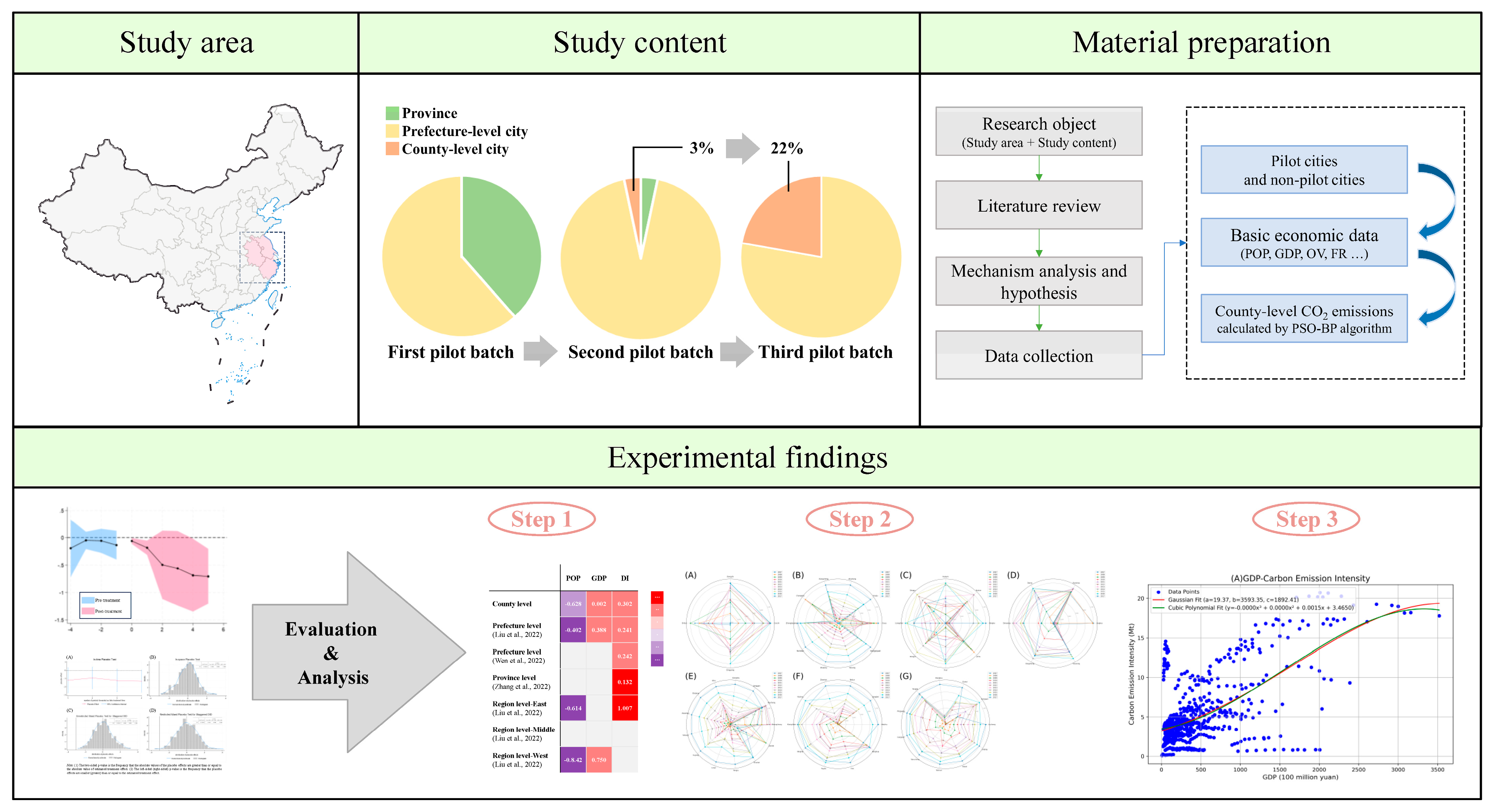
Figure 1 depicts the research framework for this paper. The remainder of this paper is structured as follows. Section 2 introduces the analytical framework and hypotheses. Section 3 outlines the data and the staggered DID methodology. Section 4 presents the empirical results and explores the mechanisms through which the LPP influences emissions, including spatial population dynamics, industrial restructuring, and household consumption patterns. Section 5 discusses the findings in light of the existing literature and derives policy implications.

2. Mechanism Analysis

This study addresses the aforementioned methodological and spatial gap by utilizing county-level carbon emissions data measured with the most recent methodology alongside data from the China City Statistical Yearbook. By employing the staggered DID methodology, this study provides a more accurate and comprehensive assessment of the effects and mechanisms of low-carbon pilot policies on carbon emissions in county-level cities within the Yangtze River Delta region.

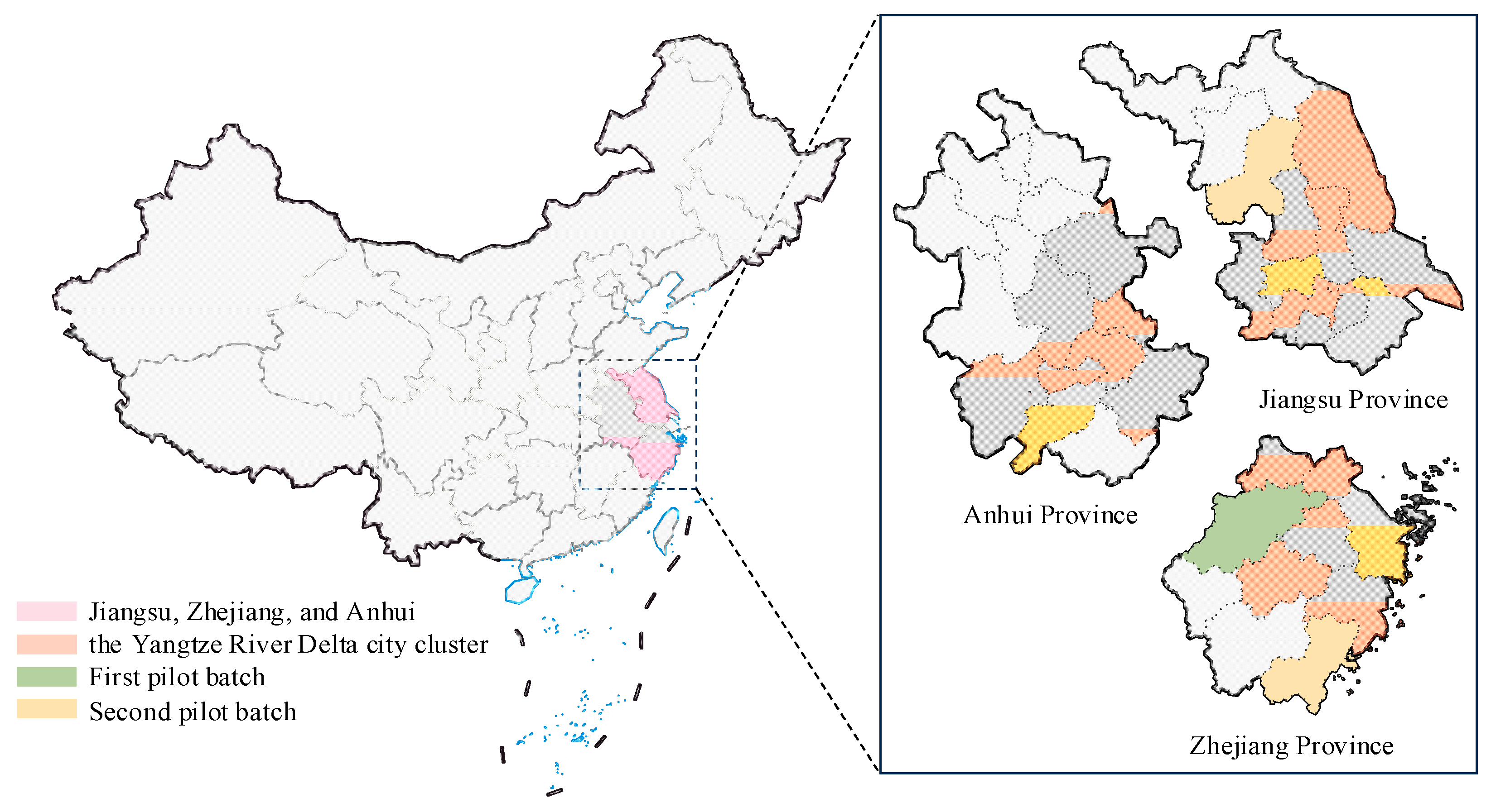
The effect of the LPP on carbon emissions was investigated using the DID model for causal analysis. The model is based on the low-carbon pilot project notices issued by the National Development and Reform Commission in 2010 and 2012. As shown in Figure 2, the treatment group consists of 51 county-level cities from the 7 prefecture-level cities designated as low-carbon pilot cities, while the control group comprises 57 other county-level cities within the Yangtze River Delta city clusters.

LPP initiatives have prompted local governments to create implementation plans tailored to their regional economy and distinct characteristics. These plans include setting up environmentally friendly systems in industry, energy, construction, and transportation contexts; developing supportive rules for green growth; instituting systems for collecting and managing greenhouse gas emissions data; and vigorously promoting pro-environmental lifestyles and behavior. The LPP is extensive and varied, integrating both financial incentives and regulations pertaining to the environment [8]. For example, the Zhenjiang government utilized CNY 158 million from the central government’s fiscal funds. It also employed other financial tools, such as tax incentives and favorable financing, to steer companies towards environmentally friendly transformations. As part of its low-carbon strategy, Suzhou aimed to implement several key regulatory measures. These included launching a greenhouse gas emissions management platform, a low-carbon product certification system, and a carbon reporting system for major enterprises. The city’s ultimate goal was to launch a carbon emissions trading platform by 2025.

Based on the aforementioned points, we argue that in principle, the LPP should effectively reduce emissions in county-level cities. Therefore, this study proposes the following hypothesis: the implementation of the LPP reduces carbon emissions.

3. Methodology

3.1. Model Development

We employ a staggered DID model to estimate the impact of the LPP on county-level emissions. This approach is particularly suitable because the policy was implemented at different times across counties, allowing us to exploit the temporal and cross-sectional variation simultaneously. Compared with a standard two-period DID, the staggered design enables a more accurate estimation of dynamic treatment effects and heterogeneity in policy timing, which are central to our research question. The model utilized, shown in Equation (1) below, is a staggered DID regression equation that includes both time and individual fixed effects and treatment and event time indicators. As Goodman-Bacon illustrates, the static staggered DID two-way fixed effects treatment effect estimate represents a weighted average of all potential two-group and two-period DID estimators (2 × 2 DIDs) in the dataset [21]. In some of these 2 × 2 DIDs, units that have already received treatment can act as comparison units for those receiving treatment later, leading to a “bad comparisons” problem when treatment effects vary across cohorts or over time. Additionally, Sun and Abraham emphasize that in two-way fixed effects dynamic effect estimation, the estimator for one relative time period can be affected by causal effects from other periods [23]. This indicates that event study designs cannot adequately address the issue of heterogeneous treatment effects.

The formula for estimating the effect, referencing Goodman-Bacon and Sun and Abraham [21,23], is given by Equation (1):

$$Y_{it}=\mathrm{\alpha }+{\mathrm{\lambda }}_t+{\theta }_i+\sum _{g\ne c}{\beta }_g\ast D_{it}^g+\sum _{k=-K}^K{\gamma }_k\ast L_{it}^k+{\epsilon }_{it}$$

(1)

The following provides a detailed explanation of the components and their roles in the model: Explained variable $Y_{it}$ represents the carbon emissions for individual county-level city (i) at time (t). Time fixed effect ${\mathrm{\lambda }}_t$ captures the overall changes that occur at each time point, controlling for common shocks to all individuals at t. Individual fixed effect ${\theta }_i$ accounts for time-invariant characteristics of each county-level city, capturing fixed differences across individuals. Treatment group indicator $D_{it}^g$ equals 1 if individual county-level city is in treatment group g at time t and 0 otherwise. Treatment group g refers to the group of individuals that receive the treatment at the same time. Treatment effect ${\beta }_g$ measures the effect of being in treatment group g. Different treatment groups can have different effects. Event time indicator $L_{it}^k$ equals 1 if the distance between t and the time of treatment for individual i is k periods. Here, k can be negative (before treatment), zero (during treatment), or positive (after treatment). Event Time Effect ${\gamma }_k$ captures the dynamic effects of the treatment at different time points relative to the treatment time. ${\epsilon }_{it}$ denotes the random disturbance term.

3.2. Variable Description

Explained variable is carbon emissions. Chen calculates carbon emissions by combining energy-related CO₂ emissions with the carbon sequestration values of terrestrial vegetation [25]. It employs three sets of satellite data, including nighttime light data from Defense Meteorological Satellite Program Operational Linescan System and National Polar-Orbiting Partnership Visible Infrared Imaging Radiometer Suite (data provided by NASA and NOAA), as well as net primary productivity data from Moderate Resolution Imaging Spectroradiometer (data provided by NASA-MOD17A3). The formula for estimating CO₂ emissions is given by Equation (2):

$$C_E^t=\sum _{i=1}^{30}{C}_{Direct,1}^t=\sum _{i=1}^{30}\sum _{j=1}^{17}\left[E_{ij}^t\ast {LCV}_{ij}^t\ast {CC}_{ij}^t\ast {COF}_{ij}^t\ast {\displaystyle \frac{44}{12}}\right]$$

(2)

where $C_{E,i}^t$ represents the provincial emissions from energy use (measured in million tons); $E_{ij}^t$ is the amount of the jth type of energy used in province i. ${LCV}_{ij}^t$ is the low calorific value of the jth type of energy consumed. ${CC}_{ij}^t$ is the carbon content of the jth type of energy source. ${COF}_{ij}^t$ is the carbon oxidation factor of the jth type of energy source. The factor $44/12$ is the ratio of the molecular weight of CO₂ to carbon.

These data were preprocessed to address issues such as discontinuities and noise. This study employed a Particle Swarm Optimization–Backpropagation (PSO-BP) algorithm to downscale provincial energy-related carbon emissions to the county level, using nighttime light data as a proxy for human activities. Furthermore, it calculates the carbon sequestration of various vegetation types, such as forests and grasslands, using established conversion coefficients. The PSO-BP algorithm integrated the different satellite data sources, generating accurate county-level estimates of CO₂ emissions and sequestration. These high-resolution estimates are crucial for developing effective, localized emission reduction policies in China.

Following Liu [13], city-level control variables include city’s economic development level, population size, industry structure, consumption patterns, and general public financial revenue. Proxy indicators for all these variables are listed in

Table 1. Descriptive statistics for the sample cities.

	Obs (% Missing)	Total (N = 1188)				Pilot Cities (N = 561)				Non-Pilot Cities (N = 627)
		Mean	SD	Min	Max	Mean	SD	Min	Max	Mean	SD	Min	Max
Explained variable
CE Carbon emissions	1188 (0)	5.34	4.23	0.09	20.73	5.46	4.60	0.09	20.73	5.18	3.63	0.19	19.08
City-level control variables
POP Population	1166 (1.9)	61.72	31.89	10.83	143.69	58.36	30.61	10.83	134.83	66.46	33.05	14.94	143.69
GDP Gross domestic product per capita of cities	1089 (8.3)	440.03	488.52	6.7	3250.35	500.67	566.71	6.7	3250.35	364.22	354.42	13.33	2260.27
OV Output value of industrial enterprises above designated size	1078 (9.3)	825.03	1141.95	5.48	8481.92	899.72	1346.52	5.73	8481.92	733.35	816.38	5.48	4982.92
FR Financial revenue	1088 (8.4)	39.18	51.34	0.58	325.51	47.44	62.28	0.633	352.51	28.88	30.73	0.58	226.46
TRS Total retail sales of consumer goods	1078 (9.3)	141.28	146.91	3.63	945.85	156.56	165.24	3.63	945.85	122.52	118.16	5.42	653.79
DI Disposable income of urban residents	1078 (9.3)	2.69	1.18	0.24	6.61	2.81	1.29	0.24	6.05	2.54	1.02	0.93	6.61

Notes: The sample size (N), mean, and standard deviation (SD) of each variable are included in this table together with other descriptive statistics of the estimation sample. Million tons is the unit of carbon emissions. The Gross Domestic Product per capita of cities (GDP), output value of industrial enterprises above designated size (OV), financial revenue (FR), and total retail sales of consumer goods (TRS) are reported in CNY 100 million Chinese (CNY), whereas the unit of disposable income of urban residents (DI) is ten thousand CNY per person, and the unit of urban population is 10,000 persons.

. Data for county-level control variables were sourced from the China City Statistical Yearbook, published by the National Bureau of Statistics.

3.3. Descriptive Statistics

Table 1 provides summary statistics for the sample cities. We have divided our sample into three categories: all cities, pilot cities (the treatment group), and non-pilot cities (the control group). As shown in Table 1, disparities exist between treatment group and control group. Specifically, pilot cities exhibit slightly higher average level of carbon emissions but a marginally lower average population level than non-pilot cities do. To ensure the validity of our causal inference, we subsequently conduct a parallel trend test to assess whether the treatment and control groups follow similar trends prior to policy implementation.

3.4. Bacon Decomposition

As discussed in the model development section, heterogenous treatments and variation in treatment timings complicate the definition of pre- and post-treatment periods. They also make it challenging to define the average treatment effect on the treated (ATT), as simply averaging treatment sizes, as is performed in standard two-way fixed effects models, is no longer valid. A key insight of new DID methodologies is that the relative grouping of treated and untreated units, as well as early- and late-treated units, matters significantly. Each combination of these groups contributes uniquely to the overall average treatment effect, denoted as β. This is precisely what the Bacon decomposition elucidates. It breaks down the β coefficient into a weighted average of β coefficients calculated from 3 different 2 × 2 combos below:

(1)

Treated (T) vs. never treated (U);

(2)

Early treated (T^e) vs. late control (C^l);

(3)

Late treated (T^l) vs. early control (C^e).

Figure 3A displays the results of the Bacon decomposition for our sample, where each plotted point represents one of the three types of 2 × 2 comparisons: The treated versus never treated (T vs. U) is shown as a triangle. Crosses represent late versus early treated (T^l vs. T^e) combinations. The hollow circle represents the timing groups or early versus late treatment groups (T^e vs. T^l).

The table in Figure 3A shows that the overall coefficient of β = −0.368 is derived from the weighted average total of the various 2 × 2 comparisons among the early-treated, late-treated, and never-treated groups. This decomposition is the fundamental principle of the Bacon method.

In 2 × 2 DIDs, units that have already received treatment can act as comparison units for those receiving treatment later, leading to a negative comparisons problem if treatment effects vary during time or among cohorts. Because each city enters the low-carbon pilot program at different times, the research design of this paper includes three types of controls below:

(1)

Two pilot batches (the treatment group) versus non-pilot cities (the never-treated group).

(2)

The first pilot batch (the earlier treated group) versus the second pilot batch that has not yet entered the low-carbon pilot program (the later treated group).

(3)

The second pilot batch (the later treated group) versus the first pilot batch that has already entered the low-carbon pilot program (the earlier treated group).

Of these three controls, the first two are robust controls as they compare the effect of entering the low-carbon pilot program on carbon emissions. However, the treatment effect for the third control is not necessarily homogeneous. If the average control estimate for the third group is weighted more heavily, it can affect the results of the two-way fixed effects estimator and introduce bias. Figure 3B shows that the average control estimate for the third group is 0.36, and since its weight in the comparison is only 8.56%, it has a minimal impact on the overall estimation results.

3.5. Min–Max Scaling

Data normalization is the core principle for eliminating the influence of differing numerical magnitudes. In this study, the Min–Max Scaling method was applied to linearly transform the data into a fixed range. By assigning equal weight to all data points, this method ensures that values across different features or years are on a common scale. This facilitates the comparisons of trends rather than a focus on absolute values.

The mathematical formula for Min–Max Scaling is as follows:

$$X_{scaled}={\displaystyle \frac{X-X_{min}}{X_{max}-X_{min}}},X_{scaled}\in [0,1]$$

(3)

where

X: Original data value.

X_min: Minimum value in the current feature column.

X_max: Maximum value in the current feature column.

X_scaled: Scaled data value.

4. Empirical Results

4.1. Benchmark Regression

This regression output provides insights into the effects of various predictors on the dependent variable y. Significant predictors (DID, POP, GDP, and DI) highlight key relationships, whereas non-significant ones (OV, FR, and TRS) indicate areas with no evident impact. The model appears robust, as indicated by the high R-squared values and significant overall F-statistics.

The results of the benchmark regression analyses, which evaluate the effect of the LPP on carbon emissions, are presented in

Table 2. The impact of low-carbon pilot policy on carbon emissions.

	Carbon Emissions	T-Value	Carbon Emissions	T-Value
DID	−0.3681 ** (0.1456)	−2.51	−0.3052 ** (0.0920)	−3.32
POP			−0.6278 ** (0.0190)	−3.30
GDP			0.0021 ** (0.0006)	3.33
OV			0.0006 (0.0001)	0.45
FR			0.0058 (0.0037)	1.56
TRS			−0.0005 (0.0013)	−0.39
DI			0.3022 ** (0.1334)	2.26
City fixed effect	Yes		Yes
Year fixed effect	Yes		Yes
Observation	1188		1078
R-squared	0.9826		0.9914
Adjusted R-squared	0.9807		0.9903
F	6.31		16.06

Note: ** p < 0.05.

. County and time fixed effects were included in both models. Group (2) builds on Group (1) by incorporating city-level controls. As shown in Table 2, the coefficients for the DID terms in both groups are negative and statistically significant at the 5% level, indicating that the low-carbon policy significantly reduces carbon emissions in the pilot counties.

In Group 2, with the inclusion of city-level control variables, the magnitudes of the coefficient change, highlighting how these additional factors influence carbon emissions. This underscores the importance of including such control factors in the baseline model to better represent the overall policy’s impact. The results from Group (2) demonstrate that the adoption of the LPP effectively reduces carbon emissions. After accounting for these potential confounding variables, the LPP is associated with a 30.52% decrease in emissions for the pilot counties. Therefore, Hypothesis 1 is verified.

To test whether the marginal effect of the population differs between treated and control counties, we employed a model specification that includes an interaction term between POP and the treatment indicator. The coefficient of this interaction term measures the differential effect of population changes on emissions in pilot counties relative to non-pilot counties. The coefficient of POP reported in Table 2 should be interpreted as the average within-county association: after controlling for county and year fixed effects and other covariates, a one-unit increase in POP is associated with a 0.6278 unit decrease in county-level carbon emissions on average. Conversely, the positive coefficient for the GDP indicates that counties with a higher per capita GDP tend to have higher emissions.

4.2. Heterogeneous Treatment Effects

Callaway and Sant’Anna argued that there are four types of ATTs that can be calculated using different weighting methods: a simple weighted summation of equal weights named Simple ATT, a weighted summation grouped according to the distance from the time of the first treatment named Dynamic ATT, a weighted summation of the average treatment effect grouped by the calendar year named Calendar Time ATT, and a weighted summation of the average treatment effect grouped according to the time of the first treatment named Group ATT [22]. It is important to note that Dynamic ATT processing requires that the Pre_avg is not statistically significant while the Post_avg is significant. As shown in

Table 3. Impact of low-carbon pilot policy on county-level carbon emissions.

	Simple ATT	Dynamic ATT	Calendar Time ATT	Group ATT
ATT	−0.512 ** (0.251)
Pre_avg		−1.090 (0.137)
Post_avg		−0.448 ** (0.207)
CAverage			−0.460 ** (0.205)
GAverage				−0.470 ** (0.202)

Note: ** p < 0.05.

, the results of this study satisfy these requirements. Furthermore, the data also show significant results when estimated using the other three weighting methods.

4.3. Parallel Trend

The validity of the DID method in the benchmark regression model relies on the parallel trend assumption. This assumption requires that, prior to policy implementation, the trends in carbon emissions between county-level cities in the LPP program and those in non-pilot cities were not significantly different.

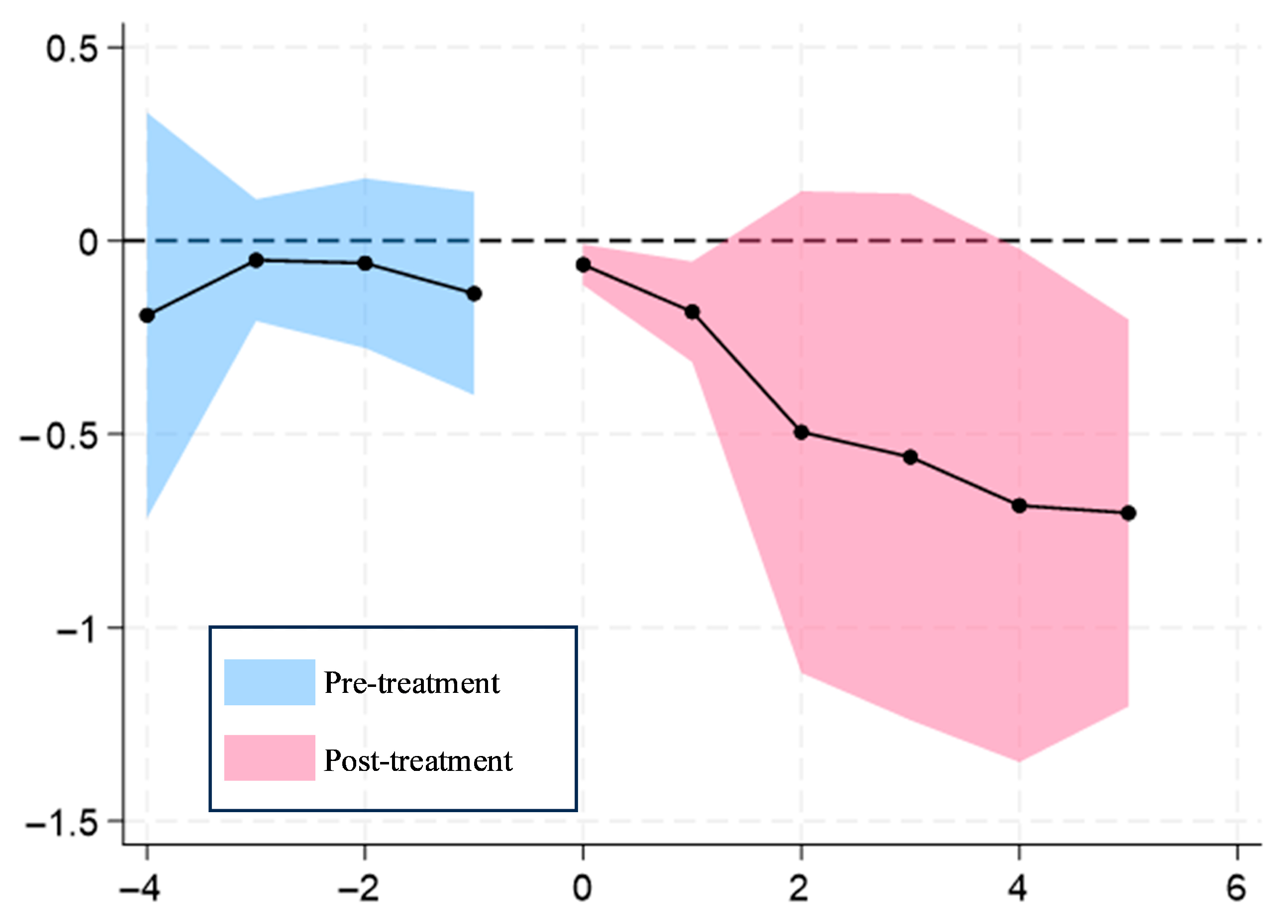
As illustrated in Figure 4, the horizontal axis represents the relative period of the LPP implementation in the target country. The year before the LPP implementation is designated as the policy base timing point, and the year of adoption is marked as 0. The vertical axis indicates LPP impact coefficients for the low-carbon pilot regions. All coefficients in Figure 4 at each time point are significant at the 95% confidence level.

Figure 4 shows that the policy impact coefficient on carbon emissions was not statistically significant before the adoption of the LPP but became significant afterward. This confirms that the carbon emission trends between pilot and non-pilot cities were similar prior to the policy’s introduction, thereby validating the parallel trend assumption. The results also indicate that the LPP had a significant reducing effect on emissions. Figure 4 also illustrates that the policy effect on reducing county-level carbon emissions reductions is sustainable and tends to stabilize over time.

4.4. Placebo Tests

Chen et al. recommend implementing placebo tests when estimating DID models, particularly in cases of synchronized or staggered policy adoption [26]. In this study, we conducted several placebo tests to ensure robustness. These include the following:

In-time placebo tests, which use fake treatment times.

In-space placebo tests, which use randomly selected fake treatment units.

Mixed placebo tests, which use both randomly selected fake treatment units and times.

We also produced corresponding graphs for visualizing the results of these tests.

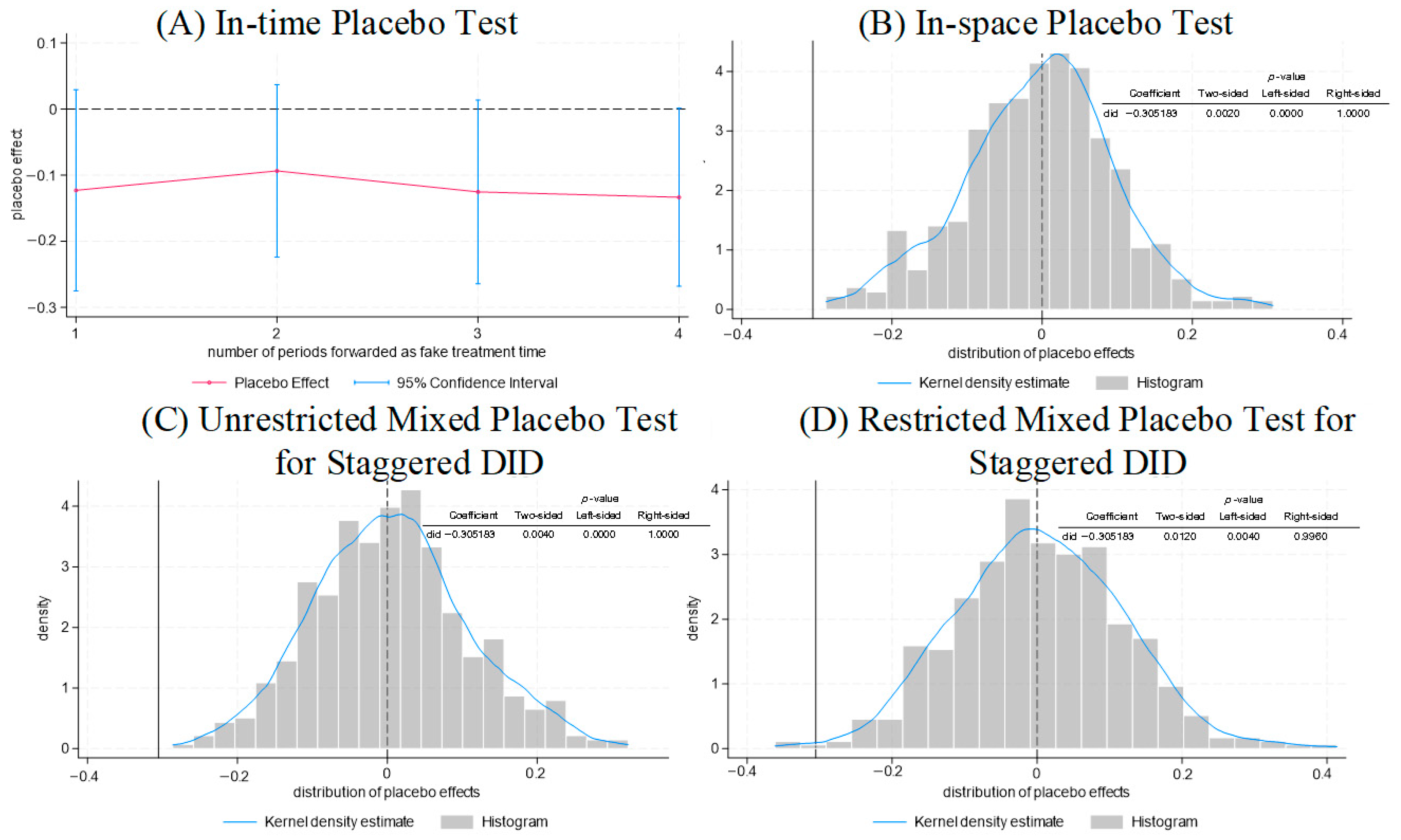
Figure 5A presents the results of the placebo test by shifting the treatment time forward by one to four periods, and it also plots the 95% confidence intervals for the time placebo effect. The results indicate that all placebo effects were not significant.

Figure 5B displays the two-sided, left-sided, and right-sided p-values for the spatial placebo test. The two-sided p-value is 0.002 (significant at the 5% level), and the left p-value is 0.000 (significant at the 1% level), leading to the rejection of the null hypothesis that the treatment effect is 0. For a more intuitive interpretation, a kernel density plot and a histogram of the placebo effect are included. These show that the treatment effect estimate (the solid vertical line in the plots) falls in the left tail of the placebo effect distribution, indicating it is an extreme outlier.

Figure 5C illustrates the results of an unrestricted mixed placebo test, which employs both pseudo treatment units and pseudo treatment times. Specifically, the pseudo treatment times for each city were randomly selected from a uniform distribution spanning the earliest and latest times of the low-carbon pilot projects in the sample. Two-way fixed effects estimations were conducted over 500 repetitions to generate the distribution of the placebo effects. Figure 5C shows the p-values, with a two-sided p-value of 0.004 and a left p-value of 0.000, again strongly rejecting the null hypothesis of no treatment effect. For a visual representation, the analysis includes kernel density plots and histograms of the placebo effects. The estimated treatment effect (the solid vertical line in the plots) is located at the extreme left tail of the placebo effect distribution, confirming its status as a significant outlier.

It is evident that conducting an unrestricted mixed placebo test disrupts the original grouping structure of staggered DID models (i.e., the number of units within each group). To address this, we proceed with a restricted mixed placebo test to maintain the grouping structure of the staggered DID (i.e., keeping the number of units within each group the same as in the original sample). The table in Figure 5D above presents the two-sided, left-sided, and right-sided p-values from the restricted mixed placebo test. The two-sided p-value is 0.012, and the left-sided p-value is 0.004, decisively rejecting the null hypothesis that the treatment effect is 0. For visual clarity, the analysis includes kernel density plots and histograms of the placebo effects. The estimated treatment effect, depicted by the vertical solid line in the plots, is positioned in the left tail of the placebo effect distribution, indicating that the observed treatment effect is extreme.

4.5. Additional Analyses

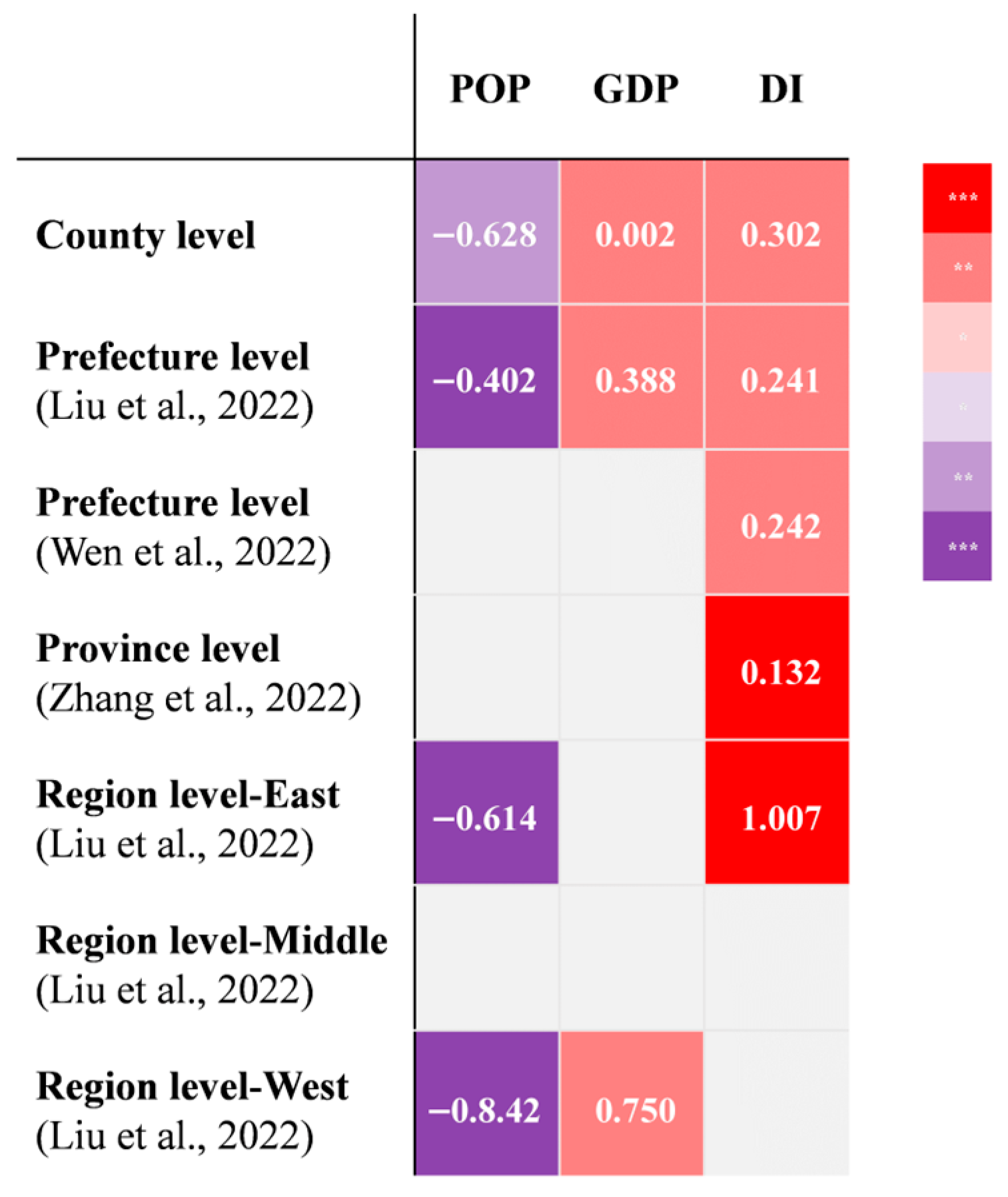
To further examine the mechanisms underlying emission changes, we compare the relative influence of key control variables at different county levels. Figure 6 shows the standardized regression coefficients for the main control variables across these levels, which allow for a direct comparison of their magnitudes. This analysis underscores the distinctive role of county-level dynamics in shaping carbon emissions.

In particular, the impact of the population density is consistently negative and relatively larger in magnitude at the county and pilot county levels. This suggests that population shifts associated with industrial upgrading in suburban counties contribute more significantly to emission reductions at finer administrative scales. In contrast, the coefficients at regional and prefecture levels are smaller in magnitude, reflecting more aggregated effects that obscure these localized dynamics.

This multiscale comparison provides additional evidence supporting our main argument that county-level governance captures emission drivers that are often masked at higher administrative levels.

Unlike the United States, where federal policy drives carbon reductions through a bottom-up approach, China’s central government initially took a leading role in its low-carbon pilot programs. Drawing on the practical experience of the United States, a lack of local government capacity typically results in less effective emission reductions compared to uniform national regulation [27,28]. Therefore, by comparing the influence of different control variables on policy outcomes across various administrative scales in the benchmark regression results, we can identify the key factors that support the implementation of carbon emission reduction policies by county governments.

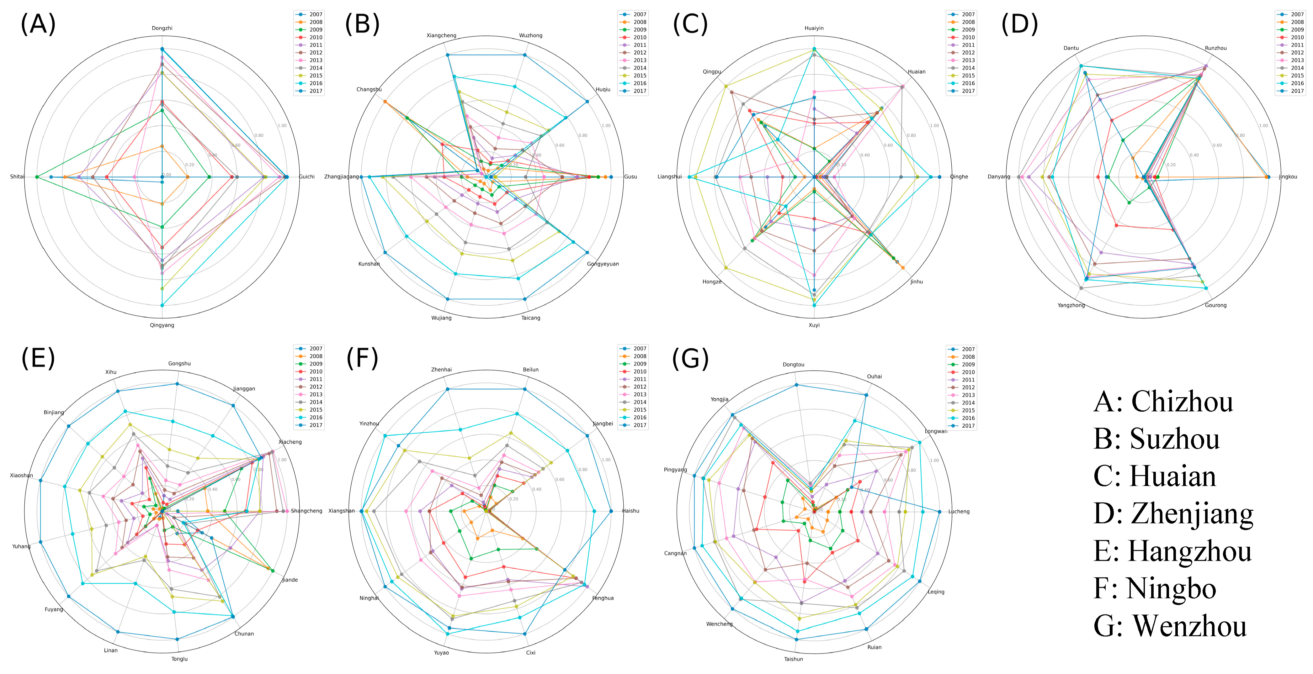
As shown in Figure 6, population density plays an important role in reducing carbon emissions at the regional, prefecture, and county levels. The radar charts of the normalized data from the pilot cities reveal a strong similarity in the regional population distribution: stable population levels in the central counties of prefecture-level cities, rapid growth in surrounding counties, and stagnation in distant suburbs.

In this figure, different colored lines represent different years, while the radius (R) from the center indicates the normalized population proportion at different scales. By plotting the population data in a radial coordinate system, Figure 7 illustrates the evolution of county populations over time. In low-carbon pilot cities in the Yangtze River Delta, central counties (e.g., Shangcheng in Hangzhou, Dantu in Zhenjiang, and Guichi in Chizhou) exhibit low variability and minimal deviation after normalization. This indicates stable population growth in these counties, which serve as economic, cultural, and transportation hubs of the state.

Counties surrounding the central areas show larger fluctuations in the normalized data, reflecting rapid population growth, especially within industrial clusters and high-tech industrial parks. These areas act as engines of industrial upgrading, attracting populations without imposing additional pressure on carbon emissions.

Conversely, distant suburban counties, such as Changshu in Suzhou, exhibit negative deviations in population growth, indicating relative stagnation or even decline. This is largely attributable to the withdrawal of traditional high-emission industries.

This pattern carries significant distributional and equity implications. While the withdrawal of high-emission firms contributes to overall emission reductions, it can also lead to population stagnation and economic decline in remote counties that were dependent on these industries. Without complementary development policies, these areas risk being marginalized in the low-carbon transition. These dynamics highlight a potential spatial inequality induced by the LPP: emission reductions are achieved partly through the geographic shift in economic activity. This shift tends to benefit central and suburban counties while imposing adjustment costs on more remote areas. Addressing these uneven impacts requires targeted regional development strategies to ensure a just transition to net-zero emissions.

To better understand the mechanism through which the LPP affects county-level carbon emissions, we examine the relationship between economic development and emissions using the Environmental Kuznets Curve (EKC) framework. If pilot counties are moving toward or beyond the EKC turning point, it indicates that the LPP may accelerate the decoupling of economic growth from emissions. Conversely, if counties remain on the upward sloping segment of the curve, it suggests that economic growth continues to drive emissions upward, despite the policy implementation. Figure 8 shows the empirical basis for this assessment.

The GDP also has a significant effect on carbon emission reductions, particularly in areas with lower levels of carbon emissions or where the speed of economic development is prioritized over its quality [29]. Focusing on the pilot counties in the Yangtze River Delta, we observe that while GDP growth generally increases carbon emissions, the rate of the increase at the county level is markedly smaller than that at the prefecture level. Both the Gaussian and cubic polynomial fits suggest that county-level cities in the Yangtze River Delta align with the EKC hypothesis. Figure 8A indicates that the Yangtze River Delta is approaching a turning point where environmental pollution stabilizes or declines with further GDP growth. In contrast, Figure 8B suggests that at the county level, the relationship between income and emissions remains on the upward trajectory, associating a higher income with higher emissions. This pattern is consistent with a high-carbon consumption phase, although additional micro-level evidence on household energy use and consumption behavior is needed for confirmation. The analysis reveals a key limitation of the low-carbon pilot program (LPP): while it has successfully reduced production-side emissions, it has not yet decoupled household consumption from carbon-intensive patterns. This underscores the need for the current policy framework to evolve its current focus on industrial and energy structures. To sustain emission reductions in the long run, policies must go beyond production to influence household consumption patterns through information campaigns, incentives for low-carbon lifestyles, and green product promotion. Integrating these demand-side measures into the LPP framework could significantly enhance its overall effectiveness.

5. Conclusions and Policy Implications

5.1. Conclusions

China’s Low-Carbon City Pilot Program has been operational for over a decade. This study provides a retrospective analysis of its effects on carbon emissions in county-level cities within the Yangtze River Delta, employing a staggered Difference-in-Differences (DID) approach.

This study empirically investigates the impact of low-carbon pilot city policies on carbon emissions using a quasi-natural experiment approach with county-level carbon emissions data measured by the latest methodology. After controlling for city-level variables, the baseline model estimates a statistically significant policy effect coefficient of −0.3052 at the 5% level, indicating that the policy significantly stimulates emissions reductions. This finding is robustly validated through a series of tests, including Bacon decomposition, heterogeneous treatment effects, parallel trend tests, and placebo tests.

Compared with earlier studies, which report moderate effects across China, the Yangtze River Delta shows a notably stronger policy impact, reflecting the higher responsiveness of economically developed regions [13]. The program also generates spatial spillovers to neighboring non-pilot cities, although these effects diminish over time, consistent with the temporal decay pattern of spatial diffusion [6,30].

Overall, the analysis reveals that the LPP in the Yangtze River Delta exhibits the following characteristics: a rapid response speed, an effective emission reduction, and a demonstrative effect on neighboring non-pilot cities. Nevertheless, significant abatement potential remains in the residential sector [31], which contributes over 30% of China’s total and more than half of its indirect emissions [32]. As economic growth and living standards rise, consumption-based emissions are expected to increase. Therefore, in addition to industrial upgrading, policies should also emphasize green consumption. Understanding household behavioral mechanisms is essential for advancing demand-side emission reduction and achieving net-zero targets. Expanding the empirical scope to diverse regions and populations will enhance the generalizability of findings and provide a stronger basis for designing targeted low-carbon policies.

5.2. Policy Implications

Based on the findings of this study, we highlight several implications in formulating pro-environmental regulations and promoting a national green growth trajectory.

First, the Chinese government should expand and refine the LPP framework to sustain and scale up its proven effectiveness. National coordination mechanisms can facilitate the diffusion of best practices from pilot regions and strengthen interregional cooperation.

Second, to prolong policy effects, supportive measures should accompany emission control initiatives. These include optimizing urban population distribution, addressing income inequality [33], and promoting green innovation to sustain long-term low-carbon development. Inter-jurisdictional collaboration can also enhance spillover benefits across administrative boundaries.

Third, public participation remains crucial. Strengthening environmental awareness through education, incentive mechanisms, and communication via digital media can motivate behavioral change and foster low-carbon lifestyles.

Finally, when devolving policy responsibilities from prefecture to county levels, potential inconsistencies and carbon leakage risks must be addressed [34,35]. The relocation of carbon-intensive industries and uneven entrepreneurial responses highlight the need for coordinated regional planning to ensure balanced and inclusive low-carbon transitions.

As global environmental governance increasingly emphasizes local action [7], this study provides a critical foundation for evaluating low-carbon policies within the specific political context of county-level governments.