Article

Vegetation Coverage Evolution Mechanism and Driving Factors in Dongting Lake Basin (China), 2000 to 2020

1
School of Geographical Sciences and Tourism, Jilin Normal University, Siping 136000, China
2
College of Resources and Environment, Fujian Agriculture and Forestry University, Fuzhou 350002, China
*
Author to whom correspondence should be addressed.
Sustainability 2025, 17(23), 10543; https://doi.org/10.3390/su172310543
Submission received: 3 October 2025 / Revised: 17 November 2025 / Accepted: 18 November 2025 / Published: 25 November 2025
(This article belongs to the Section Sustainable Forestry)

Abstract

The Dongting Lake Basin (DLB), a region of key importance in the national project of the Yangtze River Protection and Economic Belt Construction, experienced dramatic land use changes caused by anthropogenic disturbances and climate change. Understanding vegetation dynamics is crucial for improving ecosystem structure and function and environmental sustainability. Here, a long-term (2000–2020) Normalized Difference Vegetation Index (NDVI) dataset, integrated with multiple statistical methods, was applied to investigate the spatiotemporal characteristics of vegetation coverage in the DLB. The Geodetector model and partial correlation analysis were then applied to determine the main factors affecting spatial and temporal vegetation coverage change. The results showed the following: (1) The DLB showed an overall increasing NDVI at a rate of 0.37% per year from 2000 to 2020; NDVI dynamics shifted in 2010, changing from a slow to a significant increase. The seasonal average NDVI increased differently among the four seasons, in the following descending order: winter (0.56%) > spring (0.22%) > summer (0.17%) > autumn (0.05%). (2) The area with an upward NDVI trend was primarily distributed in the forest zones in the eastern and western parts, accounting for 87.55% of the total area, whereas the area with a decreasing trend was mainly clustered in the northern plains of the DLB, accounting for 6.27% of the total area. (3) The annual variation rate of the NDVI during 2010–2020 was faster than that from 2000 to 2010; the gains and losses of the transmission area were varied among different vegetation levels. (4) The DEM and slope comprised a stronger influence on the NDVI spatial variation, while the annual average temperature was the controlling climate factor, with a q-value of 26.09%. The interaction of each independent factor showed a strengthening effect for explaining the spatial variability of the NDVI. (5) Climatic factors exerted a positive correlation with the NDVI, and the temperature had a stronger influence on vegetation coverage change than that of precipitation. These results can guide the development of ecosystem models to enhance their predictive accuracy, which can provide a scientific basis for the sustainable management of vegetation resources.

1. Introduction

As a fundamental component of terrestrial ecosystems, vegetation connects the soil, atmosphere, water, and other elements in the biosphere through respiration and photosynthesis [1,2]. The awareness of vegetation dynamics attracted international environmental attention because scientists further illustrated the relationship between vegetation changes and global warming, forest degradation, and biodiversity loss [3]. Vegetation change is a complex process significantly affected by multiple variables, including topographical factors, climate change, and human activities [4], and is especially sensitive to environmental changes. The spatiotemporal characteristics of vegetation can directly reflect the health of the regional ecological environment to a certain extent [5], and monitoring dynamic changes in vegetation coverage is crucial for understanding ecological processes and formulating effective strategies for sustainable environmental management [6,7].
Remote sensing technology and satellite data have become a powerful tool for continuously monitoring land surface changes and an indispensable resource for environmental evaluation, respectively [8]. This makes it possible to globally monitor vegetation dynamics on a temporal scale [9]. The Normalized Difference Vegetation Index (NDVI), an important indicator reflecting the growth of surface vegetation, is based on the spectral information that the high reflection and strong absorption of vegetation lie in the near-infrared band and red bands. To date, it has been proven to be a successful indicator of the inter-annual attributes of vegetation coverage at regional and global scales [10,11,12]. Alternatively, long NDVI time series data were widely utilized to monitor long-term vegetation dynamics [13,14], among which the NDVI derived from the Moderate Resolution Imaging Spectroradiometer (MODIS) is favorable for monitoring the long-term variations in vegetation coverage over a long-term period due to its high temporal resolution [15].
To protect the local environment, significant efforts were undertaken to increase vegetation coverage and improve ecosystem conditions. Particularly, the catastrophic flood in 1998 prompted the awareness of ecological security imperatives by the government, leading to the implementation of a series of vegetation-related improvement strategies, including the “Grain to Green Program,” “Yangtze River Basin (YRB) Shelterbelt Construction Project”, and “Natural Forest Protection Project (NFPP),” which collectively cover the majority of central and southern China [16]. These anthropogenic activities and natural climate change may have direct or indirect influences on the terrestrial ecosystems in the YRB area. A significant increase in vegetation coverage was detected in most parts of China using long-term NDVI data. However, as highlighted by Cao [17], large-scale afforestation may increase environmental degradation in semiarid regions because planting trees in these areas influences hydrology and soil moisture. Therefore, a comprehensive understanding of vegetation coverage dynamics is a crucial endeavor for decision-makers (e.g., ecologists, policy-makers, and natural resource managers) when they develop strategies for sustainable environmental construction based on future vegetation growth trends and environmental changes [18].
The Dongting Lake is considered the second largest freshwater lake in China [19] and contributes significantly to maintaining the ecological security of the YRB area and to the agricultural product supply [20]. Currently, numerous studies exist deriving many important achievements on vegetation coverage dynamics based on NDVI time series data in the Yellow [15], Haihe [21], and Huai [22] River Basins. As an important storage lake in the Yangtze River Basin, Dongting Lake performs indispensable ecological regulation functions such as flood storage and biodiversity maintenance, with environmental benefits. However, the combined influence of global climate change and the intensification of human activities [23] caused this area to experience dramatic land use and land cover changes, leading to vegetation fluctuations over a large temporal and spatial scale, particularly following the construction of the Three Gorges Reservoir. Vegetation coverage in this basin underwent a significant change [15]. Some studies were conducted to investigate the vegetation coverage in Dongting Lake, mainly focusing on the wetland vegetation dynamics [24] and a brief analysis of the driving mechanism of vegetation coverage change [25]; however, further research on the conversion mechanisms between different vegetation coverage levels and the key drivers of their spatial and temporal evolution remains limited. Therefore, it is necessary to accurately analyze the spatiotemporal dynamic changes in vegetation coverage and their main driving factors for regional vegetation restoration and sustainable environmental management.
Since a series of environmental protection strategies was implemented between 2000 and 2020, we use long-term NDVI data (2000–2020) to quantitatively analyze the spatial pattern characteristics and temporal variations in vegetation coverage in the DLB. The Theil–Sen median method was combined with the Mann–Kendall test to determine the long-term trends and periodic changes in the NDVI. The intensity analysis method, which differs from that of earlier quantitative methods, was then employed to reveal the change process and conversion pattern of different NDVI levels. Our study objective is threefold: (1) to clarify the spatial pattern and multi-year variation trends of vegetation coverage in the DLB; (2) to elucidate the dominant transformation pattern in the mutual transformation process; and (3) to investigate the main driving mechanism of vegetation coverage dynamics.

2. Materials and Methods

2.1. Study Area

The Dongting Lake Basin (DLB), located south of the Jingjiang section in the middle reaches of the Yangtze River (107°16′–114°17′ E and 24°38′–30°26′ N) [26], extends over 28.26 × 10⁴ km2 and occupies ~14% of the total territory of the Yangtze River Basin. Its administrative scope covers the majority of Hunan and parts of Guizhou, Hubei, the Guangxi Autonomous Region, and Chongqing City (Figure 1). A subtropical monsoon humid climate influences the area, with an annual average temperature of 15.6–17.5 °C and a total annual precipitation of ~1429 mm; more than 70% of the rainfall occurs between April and July [27]. The abundant hydrothermal conditions make the vegetation coverage in this area luxuriant, which is significant for regional climate regulation [28]. As a key component of the mid-Yangtze hydrological system, the study area significantly affects flood disaster mitigation [29] and biodiversity conservation [30].
Its topography is complex, and includes mountains, hills, and plains. As one of the main forest areas in southern China, vegetation in the basin is dominated by subtropical humid forests, such as evergreen needleleaf, deciduous broadleaf, and deciduous needleleaf forests. In the context of accelerating urban growth and demographic expansion, land cover changed significantly [16]. Particularly, beach reclamation in the late 1950s and artificial afforestation due to the implementation of ecological projects in the 1980s resulted in the vegetation coverage in the DLB experiencing obvious temporal and spatial changes [31], while the ecological environmental functions were also greatly degraded.

2.2. Data Source and Processing

NDVI time series data covering the entire DLB, which were freely acquired from MODIS vegetation index products (MOD13A1; https://lpdaac.usgs.gov/products/mod13a1v006/ (accessed on 20 November 2024)), were selected here, with a spatial resolution of 500 m and a 16-day temporal resolution for the period 2000–2020. This product reduces the influence of water, clouds, and heavy aerosols during data pre-processing [2]. A total of 1449 images (path/row: h28v06, h27v05, and h27v06) were originally saved in hierarchy data format (HDF). The MODIS Re-projection Tool (MRT), provided by the US Geological Survey (USGS) at http://glovis.usgs.gov/ (accessed on 21 November 2024) was employed to re-project the raw MODIS-NDVI dataset to the Albers equal-area conic projection [32]. Subsequently, the dataset was mosaicked and extracted to obtain the NDVI data for the study area [33]. The Maximum Value Composite (MVC) method [34], which eliminates the influence of the atmosphere, cloud cover, solar elevation, and scan angle, was employed to derive the monthly NDVI from 2000 to 2020 and reduce the cloud-contaminated pixels [35,36]. The harmonic analysis of time series (HANTS) was then used to smooth the raw NDVI curve to a series of sinusoidal waves [37]. Subsequently, the monthly NDVI was classified according to year and season, and the seasons were divided into spring (March, April, and May), summer (June, July, and August), autumn (September, October, and November), and winter (December, January, and February), based on the seasonal classification standard of meteorology [2].
As NDVI change is a comprehensive process influenced by several factors, 12 indicators were chosen from aspects of climate, topographical features, human activity, and soil and vegetation types. The climate data included annual precipitation, mean temperature, sunshine hours, and relative humidity, which were obtained based on daily observation data from meteorological stations across the region (http://data.cma.cn (accessed on 12 December 2024)). Then, the ANUSPLIN interpolation method was applied to interpolate the meteorological data at a spatial resolution of 500 m, setting the 250m digital elevation models (DEMs) as co-variables. Elevation, aspect, and slope were calculated using ArcGIS 10.3 based on a digital elevation model with 250 m resolution freely downloaded from the Geospatial Data Cloud (http://www.gscloud.cn/ (accessed on 12 December 2024)). The soil and vegetation type data with a 1 km resolution were obtained from the Resource and Environmental Science Data Platform (https://www.resdc.cn/data.aspx (accessed on 15 December 2024)). The population density, GDP per capita, and reforested area were selected to reflect the intensity of human activity and were acquired from the county-level Chinese Statistical Yearbook.

2.3. Methods

2.3.1. Trend Analysis

To explore the trend of the NDVI time series, Theil–Sen median analysis [38] was adopted to analyze the dynamic changes in spatially averaged NDVI, which reduces the influence of abnormal or missing data and provides a more accurate change trend for time series data [34,39]. The slope can be represented as follows:
S n d v i = Median N D V I i N D V I j j i , i < j
where the S n d v i is the dynamic trend of NDVI, i and j are the serial year numbers, with j being larger than i, and N D V I i and N D V I j represent the sequence values of NDVI at years i and j, respectively. When S n d v i > 0, an upward trend in the NDVI is implied, and vice versa, and S n d v i = 0 shows an unchanged trend. The Mann–Kendall trend test was then employed to investigate the significance of the NDVI change trend.
The Mann–Kendall test (MK), a non-parametric statistical test [40], was employed to test the significance of Sen’s Slope, in which the sample is not required to follow a certain distribution and is less affected by abnormal values. Two hypotheses, H0 and H1, were tested by using the MK test. Under H0, no significant trend was detected when the samples in the series data were randomly arranged, whereas, under H1, a monotonic tendency of ascending or declining existed in the sequences. The formulas of statistic S and Z values can be found in Geng et al. [41].
The Z value reflects the significance level of the variation in the NDVI time series. Under a given significance level α, the null hypothesis can be rejected when the absolute value of Z is greater than that of Z 1 α / 2 , which indicates that the NDVI change has a significant trend, and vice versa. In the current study, a significance level α = 0.05 was selected [8], and the Z 1 α / 2 = Z 0.975 = 1.96 .

2.3.2. Mann–Kendall Mutation Test

Here, the Mann–Kendall mutation test was adopted to identify the change point of the NDVI time series [16]. For the NDVI sequence data x n (n is the length of the sequence data), the cumulative number of x i > x j , is denoted by r i , and the statistic S k can be defined as follows:
S k = i = 0 k r i ,       ( k = 2 , 3 , 4 , , n )               r i = 1 ,       x i > x j 0 ,         e l s e                     j = 1 , 2 , ,   i
The statistic S k has a mean of E S k and a variance of v a r S k , which can be computed using the following equations:
E S k = k k 1 4
v a r S k = n n 1 2 n + 5 72
The sequential values of U F k are defined as follows:
U F k = [ S k E ( S k ) ] / v a r S k
where U F k is the forward sequence statistic estimated using the original NDVI time series data. Similarly, the inverse order of U F k is calculated as U B k . Here, the confidential level was set as α = 0.05. The intersection point of the U F k and U B k curves is the potential changing point of the trend, and it was considered significant if the intersection point passed the threshold value for a 95% significance level (±1.96). A decrease and an increase in U F k imply a negative and positive trend in the sequence data, respectively [42].

2.3.3. Coefficient of Variation

The stability and inter-annual volatility of the NDVI were analyzed using the coefficient of variation (CV), which is used to describe the relative fluctuation in geographical data [43]. The equation for CV is as follows:
C v = 1 N D V I ¯ i = 1 n ( N D V I i N D V I ¯ ) 2 n 1
where C v , N D V I ¯ , n, and N D V I i are the coefficient of variation in the NDVI time series data, mean NDVI during 2000–2020, length of the time series (21), and NDVI value at time i , respectively. A high C v value demonstrates the instability of the time series in which a large fluctuation can be found; the higher the C v , the greater the volatility in the NDVI change; otherwise, it indicates the stable status of the time series [44].

2.3.4. Intensity Analysis

Intensity analysis, as proposed by Aldwaik and Pontius [45], offers a hierarchical approach for quantitatively analyzing land use and land cover change. It is suitable for analyzing two or more categories at different levels in two or more periods. Using a transfer matrix, land use change intensity was analyzed with time, category, and transition level, with each level offering a more detailed examination [45]. Similarly, the distribution of different NDVI level changes in a region during different time periods can be similarly investigated.
The time interval level assesses whether the overall rate of NDVI changes in each time interval (St) is faster or slower than a hypothetical uniform intensity (U) across the entire study period. If St > U, then St is fast, implying that the NDVI changes faster during the time interval [Yt−1,Yt] than that if the NDVI changes were distributed uniformly during all time intervals to a temporal extent [Y1,Yt], and vice versa. Equations (7) and (8) define the change in intensity St and the uniform intensity U, respectively:
S t = c h a n g e   a r e a   d u r i n g   Y t 1 , Y t ( t o t a l   a r e a ) ( d u r a t i o n   o f   Y t 1 , Y t ) × 100 % = j = 1 J i = 1 J C t i j C t i j / j = 1 J i = 1 J C t i j Y t Y t 1 × 100 %
U = ( c h a n g e   a r e a   d u r i n g   a l l   i n t e r v a l s ) / ( t o t a l   a r e a ) d u r a t i o n   o f   a l l   i n t e r v a l s = t = 1 T 1 j = 1 J i = 1 J C t i j C t i j / j = 1 J i = 1 J C t i j Y T Y 1
The category level investigates which specific categories (e.g., land use types or NDVI levels) were particularly active or dormant in terms of gains and losses during each time interval, compared with those of a uniform intensity St during each time interval. Equations (9) and (10) provide the intensities of the gain ( G t j ) and loss ( L t i ), respectively:
G t j = s i z e   o f   g a i n   o f   j   d u r i n g   Y t 1 , Y t ( s i z e   o f   j   a t   t i m e   Y t ) ( d u r a t i o n   o f   Y t 1 , Y t ) × 100 % = i = 1 J C t i j C t j j / Y t Y t 1 i = 1 J C t i j × 100 %
L t i   = s i z e   o f   l o s s   o f   i   d u r i n g Y t 1 , Y t s i z e   o f   i   a t   t i m e   Y t 1 d u r a t i o n   o f   Y t 1 , Y t × 100 % = j = 1 J C t i j C t i i / Y t Y t 1 j = 1 J C t i j × 100 %
Then, the transition level answers the question “which level is dormant in the process of mutual transformation among different categories of NDVI?” by comparing the annual transition intensity ( R t i n ) from category i to n (n   i ) with a uniform transition intensity ( W t n ) of the transition to category n from non-n category at time Y t 1 during the time interval [ Y t 1 , Y t ] . The formulas for the transition intensity are as follows:
W t n = s i z e   o f   g a i n   o f   n   d u r i n g   Y t 1 , Y t s i z e   o f   n o t   n   a t   t i m e   Y t 1 d u r a t i o n   o f   Y t 1 , Y t = i = 1 J C t i n C t n n / ( Y t Y t 1 ) j = 1 J i = 1 J C t i j C t n j × 100 %
R t i n = s i z e   o f   t r a n s i t i o n   f r o m   i   t o   n   d u r i n g   Y t 1 , Y t ( s i z e   o f   i   a t   t i m e   Y t 1 ) ( d r u a t i o n   o f   Y t 1 , Y t ) = C t i n / ( Y t Y t 1 ) j = 1 J C t i j × 100 %
If R t i n   >   W t n , then the gain of n targets i, implying that the gain of n transitions from non-n categories more intensively during the time interval Y t 1 , Y t than that if the gain of n transitioned uniformly from non-n categories at time Y t 1 , and vice versa [46].
V t m = s i z e   o f   l o s s   o f   m   d u r i n g   Y t 1 , Y t s i z e   o f   n o t   m   a t   t i m e   Y t d u r a t i o n   o f   Y t 1 , Y t = j = 1 J C t m j C t m m / ( Y t Y t 1 ) i = 1 J j = 1 J C t i j C t i m × 100 %
Q t m j = s i z e   o f   t r a n s i t i o n   f r o m   m   t o   j   d u r i n g   Y t 1 , Y t ( s i z e   o f   j   a t   t i m e   Y t ) ( d r u a t i o n   o f   Y t 1 , Y t ) × 100 % = C t m j i = 1 J C t i j × 100 %
where V t m is the uniform intensity of the transition from category m to all non-m categories at time point Y t during time interval Y t 1 , Y t and m is the NDVI categories converted to other categories. Q t m j is the annual intensity of transition from category m to category j (j ≠ m) during Y t 1 , Y t .
Intensity analysis is based on the distribution of categories at different time points and makes the best use of the transition matrix. Therefore, it requires the classification criteria of the NDVI at each time point to be consistent. Thus, according to the spatial distribution of NDVI in the DLB during 2000–2020, we defined the years 2000, 2010, and 2020 as the three time points and classified the NDVI into five levels by natural breaks [47]: low (NDVI ≤ 0.417), low–medium (0.417 < NDVI ≤ 0.652), medium (0.652 < NDVI ≤ 0.724), medium–high (0.724 < NDVI ≤ 0.808), and high (NDVI > 0.808). ArcGIS 10.3 was employed to obtain the transition matrix of different NDVI levels at two time intervals (2000–2010 and 2010–2020) (Table 1).

2.3.5. Spatial Autocorrelation Analysis

The spatial autocorrelation analysis was utilized to investigate the spatial distribution patterns of vegetation coverage in the DLB. Using ArcGIS 10.3, spatial heterogeneity and spatial clustering characteristics of vegetation coverage in 2000, 2010, and 2020 were analyzed, respectively. Through the local indicator of spatial association (LISA) map, five different clusters of vegetation coverage can be identified in the DLB region, namely High–High (HH), High–Low (HL), Low–High (LH), Low–Low (LL), and not significant [48].

2.3.6. Geodetector

The Geodetector model constituted a suite of statistical tools including factor, interaction, risk, and ecological detectors to investigate the influencing factors and their interaction relation for specific phenomena, and it is an open source model (http://www.GeoDetector.cn/ (accessed on 28 December 2024)). This model considers spatial heterogeneity rather than correlation to detect the impact of multiple factors on vegetation coverage spatial distribution; thus, the multicollinearity among independent variables does not affect the result of the factor detector.
Utilizing ArcGIS 10.6, 5000 sample points were generated across the study area. The NDVI values for 2020 were extracted to these points and used as the dependent variables for the Geodetector (GD) analysis. As the GD model requires categorical independent variables, and following the relevant literature [49,50] as well as the actual situation of the study area, the meteorological data (annual precipitation, mean annual temperature, sunshine hours, relative humidity) were discretized into eight grades using the natural breaks classification method [50]. Topographic factors including elevation, slope, and aspect were classified into nine grades, while population density, per capita GDP, and reforested area were divided into five grades. Soil and vegetation types were categorized into eight and seven grades, respectively. After removing outliers, the GD model was applied to the remaining 3280 samples.
A factor detector was employed to measure the explanatory power of each factor on the spatial variability of NDVI by calculating the q-value. The formula is as follows:
q = 1 h L N h σ h 2 N σ 2
where L represents the number of categories for a given variable X; N h and N express the number of cells in the h-th category and the entire area; and σ h 2 and σ 2 signify the variance of the NDVI in the h-th category and the whole area, respectively. q denotes the explanatory power of a given variable over the NDVI, which takes a value from 0 to 1; the greater the value, the stronger the explanatory power of the variable. In the GD model, a p value was used to determine the statistical significance of the relationship between explanatory factors and the dependent variable [47]. If the p value is less than 0.05, the factor is considered to significantly impact the spatial variation in the dependent variable.
An interaction detector was utilized to determine whether the interaction of two dependent variables increased or decreased the interpretation power of the dependent variable. The interaction types are listed in Table 2.

2.3.7. Partial Correlation Analysis

Partial correlation analysis is a statistical tool based on geolocation that measures the strength and direction of the linear relationship between two variables [21]. When the strengths between specified variables were examined, one variable is treated as a constant to independently investigate the relationship between dependent and intendent variables. Unlike that of simple correlation analysis, partial correlation statistically controls for the effects of other climatic factors. This method produces more accurate and reliable results, making it broadly utilized in regional vegetation climate research. Therefore, partial correlation analysis was employed to analyze the effect of climatic variables on NDVI temporal change. Considering the significant influence of temperature and precipitation on vegetation growth, annual average temperature and annual precipitation were selected to obtain the partial correlation coefficients through the following equation:
r x y · z = r x y r x z r y z ( 1 r x z 2 ) ( 1 r y z 2 )
where r x y · z represents the partial correlation coefficient between factors x and y after removing factor z.  r x y , r x z , and r y z are the partial correlation coefficients between x and y, x and z, and y and z, respectively. r x y · z > 0 indicates a positive correlation between x and y, and vice versa. The greater the r x y · z , the stronger the correlation between x and y.
In the partial correlation analysis, a t-test was used to test the significance of the partial correlation coefficient. By checking the t distribution table, if the t is greater than that of the critical value of a different significance level, the partial correlation is significant.

2.3.8. Validation and Accuracy Assessment

A total of 1500 validation samples were collected using the TimeSync plus 3.0 tool from Landsat TM5 (path: 123, row: 39 and 40) and Google Earth (https://earth.google.co.uk (accessed on 18 October 2025)) images according to random principle. TimeSync plus tool is designed to evaluate the quality of change maps derived from Landsat time series data [50]. The location of the samples and their changes were documented by TimeSync plus. Among 1500 validation samples, 1278 change plots and 222 stable plots were recorded to assess the accuracy of vegetation change detection. The overall accuracy for vegetation coverage change is 85.2%, which implies that the proposed method is effective for detecting vegetation coverage change.

3. Results

3.1. Spatial Distribution and Characteristic of Changing Trends of NDVI

From the annual characteristics, the vegetation coverage in the DLB was in good condition, with the highest NDVI value of 0.887, owing to its highly developed agricultural civilization. The NDVI exhibited spatial differentiation (Figure 2a), and high values of the NDVI occurred in the mountainous areas in the eastern and western parts of the DLB, whereas low values of the NDVI appeared in the central part due to intense human activities. Regions with high values (NDVI > 0.8) accounted for approximately 46% of the total area, whereas regions with low NDVI values (NDVI < 0.6) occupied only 2% of the total area and were sporadically distributed in the central plains (Figure 2b). From a vertical perspective, the NDVI in the DLB demonstrated an obvious increase in altitude from 0 to 500 m and maintained abundant vegetation coverage in the high-altitude areas (Figure 2c).
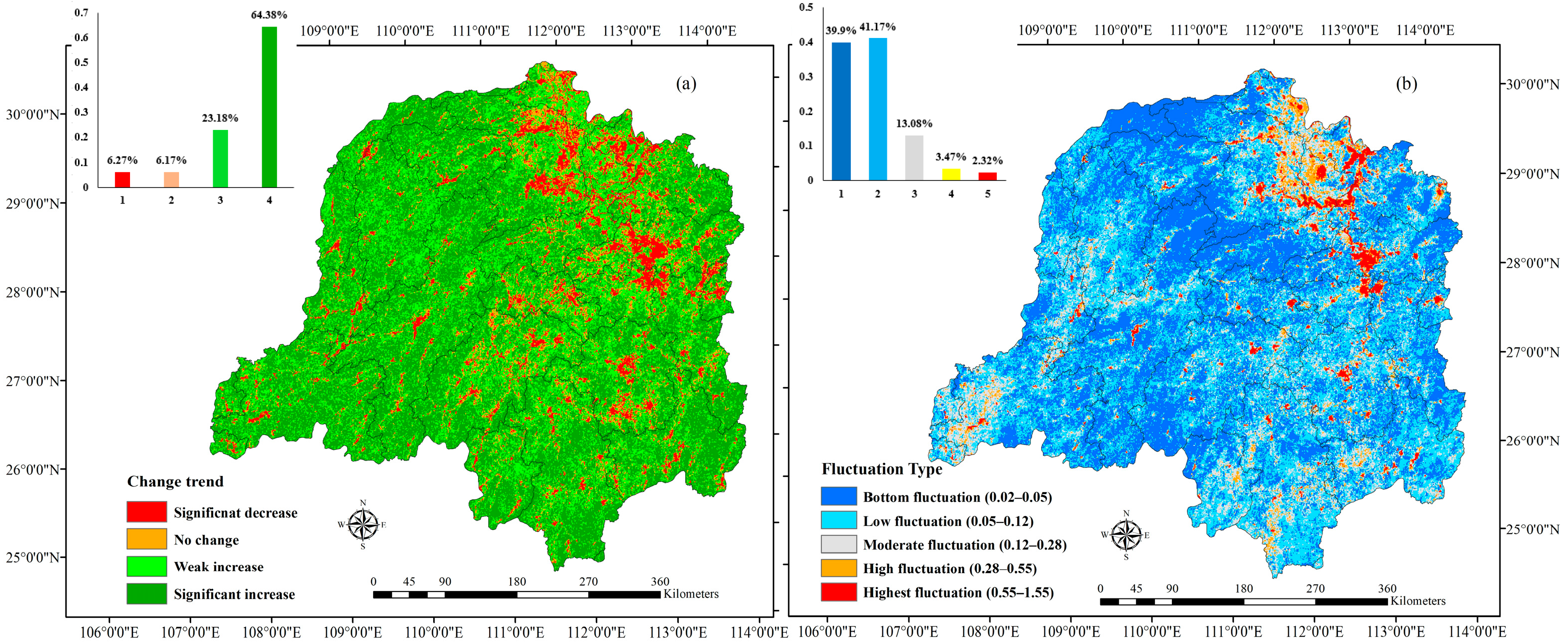
The overall trend of NDVI change from 2000 to 2020 was examined using Sen’s Slope and the M-K test at the pixel scale. With reference to the relevant research, areas with an Sndvi value between −0.0008 and 0.0008 were set as stable and unchanged. Areas with an Sndvi value greater than 0.0008 were defined as improvement zones, whereas those less than −0.0008 were designated as degradation zones. By integrating the results of the Mann–Kendall test, a spatial distribution map of NDVI trends at a pixel scale was obtained (Figure 3a). As observed from Figure 3a, the areas in which the NDVI showed an upward trend accounted for 87.55% (23.08 × 10⁴ km2) of the total study area, with areas showing a weak and significant increase occupying 23.17% and 64.38%, respectively, and being widely distributed in the forest zones covered by deciduous broadleaf forests in the eastern and western parts. Areas with significant downward trends accounted for 6.27% (1.65 × 10⁴ km2) of the total area and were mainly distributed in the northern plains of the DLB, which were dominated by wetlands and construction. Summarily, the spatial dynamic characteristics of vegetation coverage change were dominated by improvements, including weak and significant increases, whereas the downward change and no-change areas accounted for only 6.27% and 6.18% of the total area, respectively.
The coefficient of variation (CV), obtained from Equation (6), was divided into five grades using the natural breakpoint method. As illustrated in Figure 3b, the vegetation of the forested areas in the eastern and western regions showed the highest stability, with CV values ranging from 0.02 to 0.05. Comparatively, the fluctuation of the vegetation coverage of wetlands in the northern plain was considerably the highest, with the CV values ranging from 0.55 to 1.15, while lower fluctuations in vegetation were sporadically observed in the southern and southwestern regions. Overall, the vegetation dynamics differ markedly across the DLB, with the northern plains exhibiting pronounced disturbances compared to the stable conditions in the mountain regions. Seasonal variations in the water level were the primary reasons, as flood season submergence inhibits plant growth and lowers vegetation indices. Conversely, the dry season recession marks an optimal growth phase, thereby facilitating a gradual recovery in vegetation coverage.

3.2. Temproal Change of NDVI

3.2.1. Inter-Annual Changes in NDVI

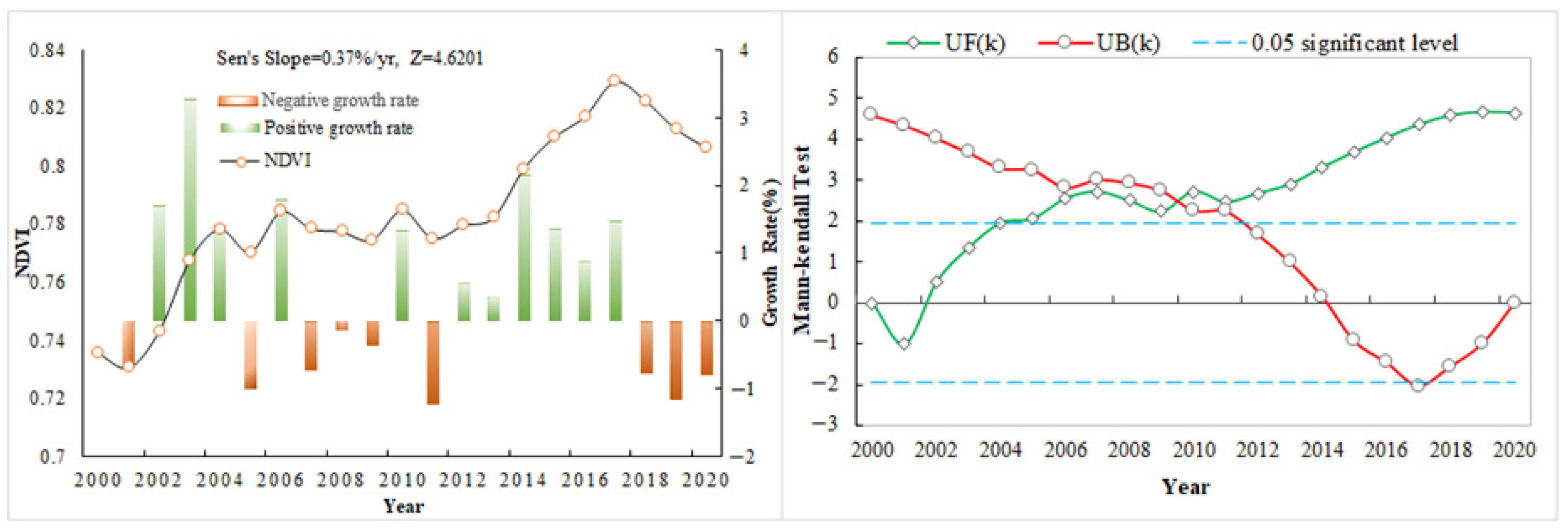
To investigate the characteristics of vegetation growth over time in the DLB, a spatial analysis in ArcGIS 10.3 was conducted to obtain the annual average NDVI, which represents the normal state of vegetation growth in that year (Figure 4). The minimum and maximum NDVI values were 0.7306 and 0.8291 in 2001 and 2017, respectively. As shown in Figure 4, the annual NDVI showed an upward trend from 2000 to 2020, with a growth rate of 0.37% per year, and passed the significance test at a level of 0.05 (Z = 4.6021 > 1.96). The changing trend in annual average NDVI values featured clear stages. The Mann–Kendall mutation test was employed to detect the characteristics of these changes. The UF statistics after 2005 exceeded the threshold value of 1.96 (at a significance level of 0.05), indicating that the NDVI showed a significant increasing trend. During this period, the upward trends in NDVI between 2005 and 2008 and 2011 and 2019 increased significantly. This may be likely due to human activities. The operation of the Three Gorges Dam in 2003 changed the hydrological regime and, coupled with ecological protection policies such as NFPP and Grain to Green, led to an uptrend in vegetation coverage. The two curves, UF and UB, intersected in 2010; therefore, the NDVI exhibited an obvious abrupt change in 2010.

3.2.2. Intra-Annual Variations in NDVI

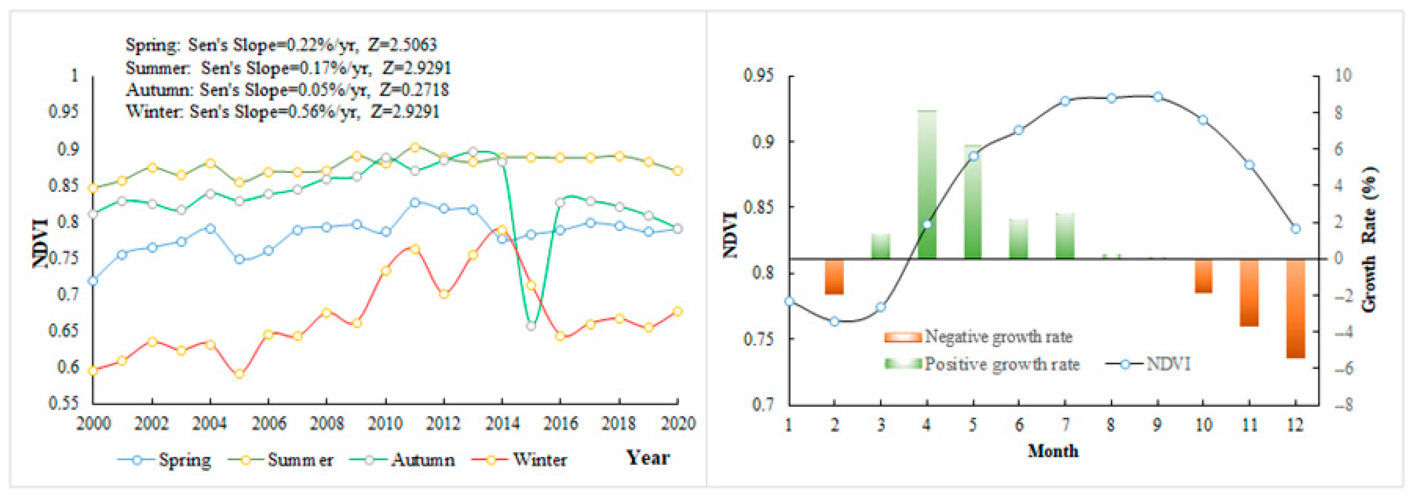
Figure 5 shows the change characteristics of the seasonal average NDVI, with the ranking features of summer (0.8772), autumn (0.8334), spring (0.7833), and winter (0.6698). Throughout the study period, the NDVI increased at rates of ~0.22% per year, ~0.17% per year, ~0.05% per year, and ~0.56% per year in spring, summer, autumn, and winter, respectively (Figure 5). The monthly average NDVI ranged from 0.7638 to 0.9338, and, consistent with the features of seasonal changes, the NDVI was relatively high during the rainy season (from May to October), with the highest value of 0.9338 appearing in September. Contrarily, a low NDVI was observed during the dry season (November–April), with the lowest value of 0.7638 in February.
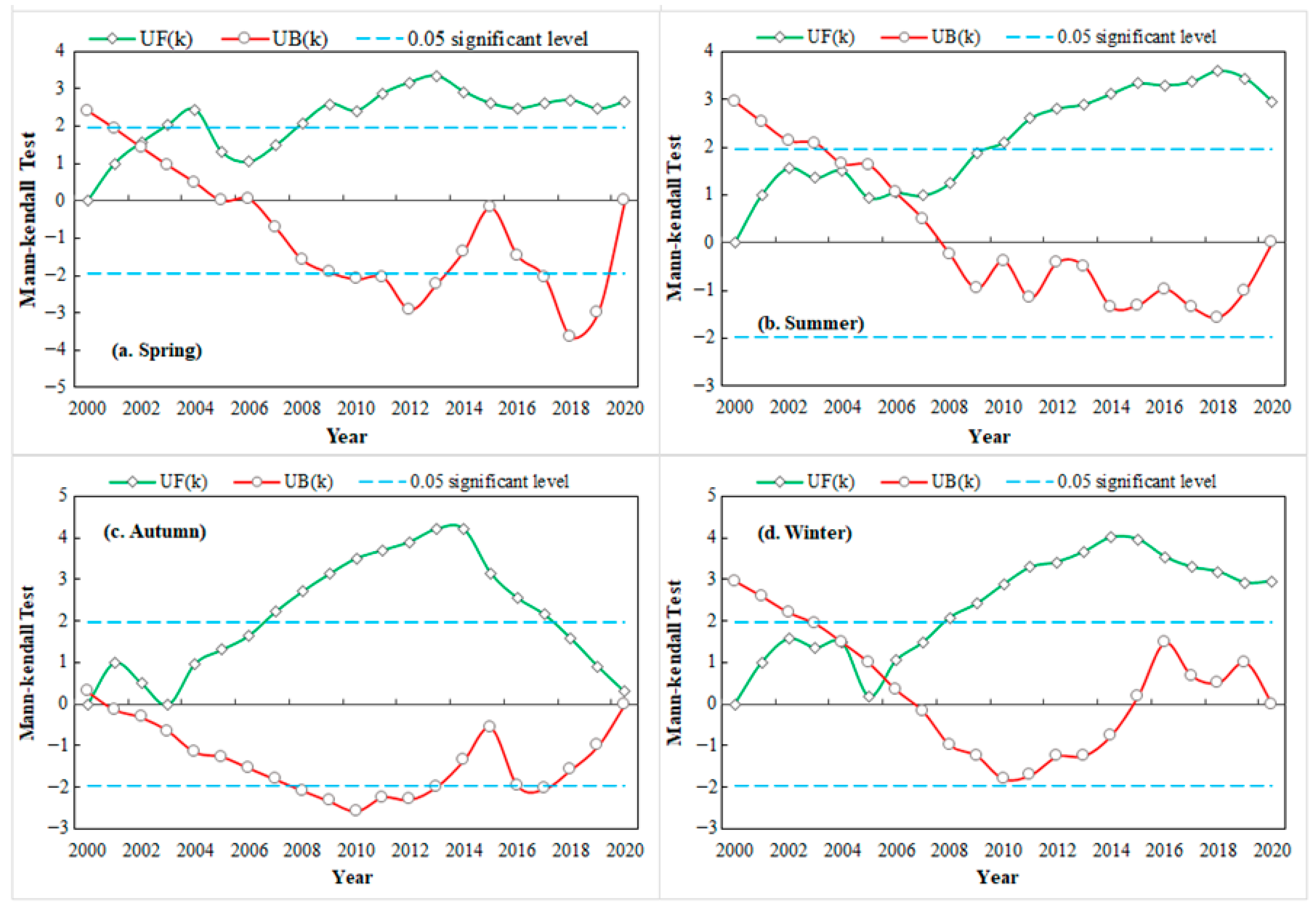
From the mutation test for each season shown in Figure 6, the NDVI in spring showed an upward trend during the time periods 2000–2004 and 2006–2013, while that during 2000–2003 was insignificant because it did not pass the critical confidence coefficient of 1.96. The NDVI in summer showed an insignificant short-term decreasing trend from 2002 to 2008. After 2010, the UF(k) value was greater than 1.96, indicating that the NDVI increased significantly, with no abrupt change after 2010, and maintained an increasing trend. The NDVI in autumn and winter comprised the same change characteristics: an insignificant declining trend from 2001 to 2005, and a change from a slow (2005–2008) to a significant (2008–2015) increase. Thereafter, the NDVI in winter decreased significantly after 2015, and the NDVI in autumn decreased significantly from 2015 to 2018 and declined non-significantly from 2018 to 2020. Abrupt changes in the NDVI in spring, summer, autumn, and winter occurred in 2003, 2006, 2000, and 2006, respectively. An abrupt change in the NDVI in spring occurred in 2003. This may be due to the construction of the Three Gorge Dam affecting the local hydrological context [51], which indirectly changed the vegetation growth. The NDVI in summer abruptly changed in 2006, possibly due to the extreme high temperature that occurred in summer [20].

3.3. Results of the Intensity Analysis

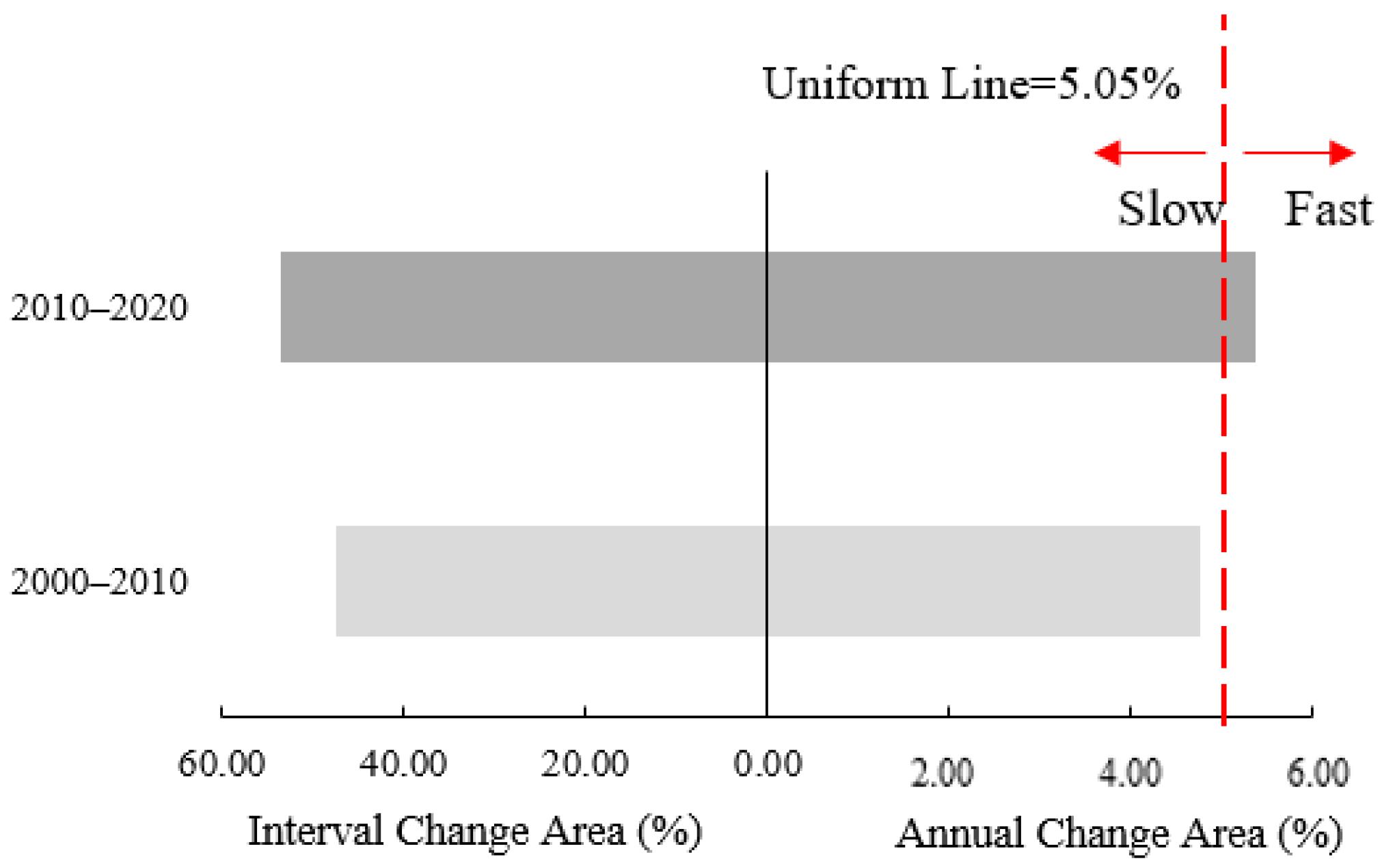
Figure 7 shows the results of the time interval intensity analysis for the two time periods 2000–2010 and 2010–2020, in which the horizontal bars on the right and the left describe the time intensity of the NDVI changes derived using Equation (7) and the overall size of the NDVI changes for each time interval, respectively. Furthermore, the dotted line indicates the uniform intensity obtained using Equation (8). If the bar exceeds the uniform intensity line, the change in NDVI during that time period is relatively fast; otherwise, it is relatively slow. As shown in Figure 7, the NDVI increased from 47.43 to 53.65% of the total area from 2000 to 2020, and the annual variation rate from 2010 to 2020 was faster than that from 2000 to 2010.
Figure 8 and Figure 9 show the results of the category-level intensity analysis, which demonstrates the size of gain and loss of each category in each time interval, indicating whether the change in each category is dormant or active. The bars on the left of the middle axis represent the gross annual changed area of each NDVI level obtained from Equations (9) and (10), whereas the bars on the right show the annual change in the intensity of gain/loss for each NDVI level. If a bar extends beyond the dashed line, then the change in the NDVI level is relatively active in the given period; if a bar stops before the dashed line, the change is relatively dormant.
From Figure 8, it is inferred that, during the time interval of 2000–2010, the annual transition changes in medium, low–medium, and low levels of NDVI gains and losses were both active, and the changing area of gains was larger than that of the losses in medium and low–medium NDVIs. The change in high-level NDVIs was dormant in terms of gain and loss, whereas the transition areas of losses were greater than those of gains. The losses in areas with high vegetation coverage were larger than those of the gains, although both were dormant. Medium–high gains were active, whereas the losses were dormant. The annual change areas of medium–high NDVI losses were greater than those of the gains and were relatively active, indicating that the medium–high vegetation coverage decreased to some extent during 2000–2010.
Figure 9 shows the results for the category intensity from 2010 to 2020. The gains and losses of the medium and low–medium NDVIs were active, and the increased areas were greater than those of the losses. The gains and losses for high NDVI levels were both dormant, and the increased and decreased areas with a high NDVI were equivalent, indicating that high vegetation coverage changed stably. The losses of the medium–high NDVIs were active and greater than those of their gains. The gains of low NDVIs were active and the losses were dormant, whereas the increasing areas were larger than those of the decreasing areas.
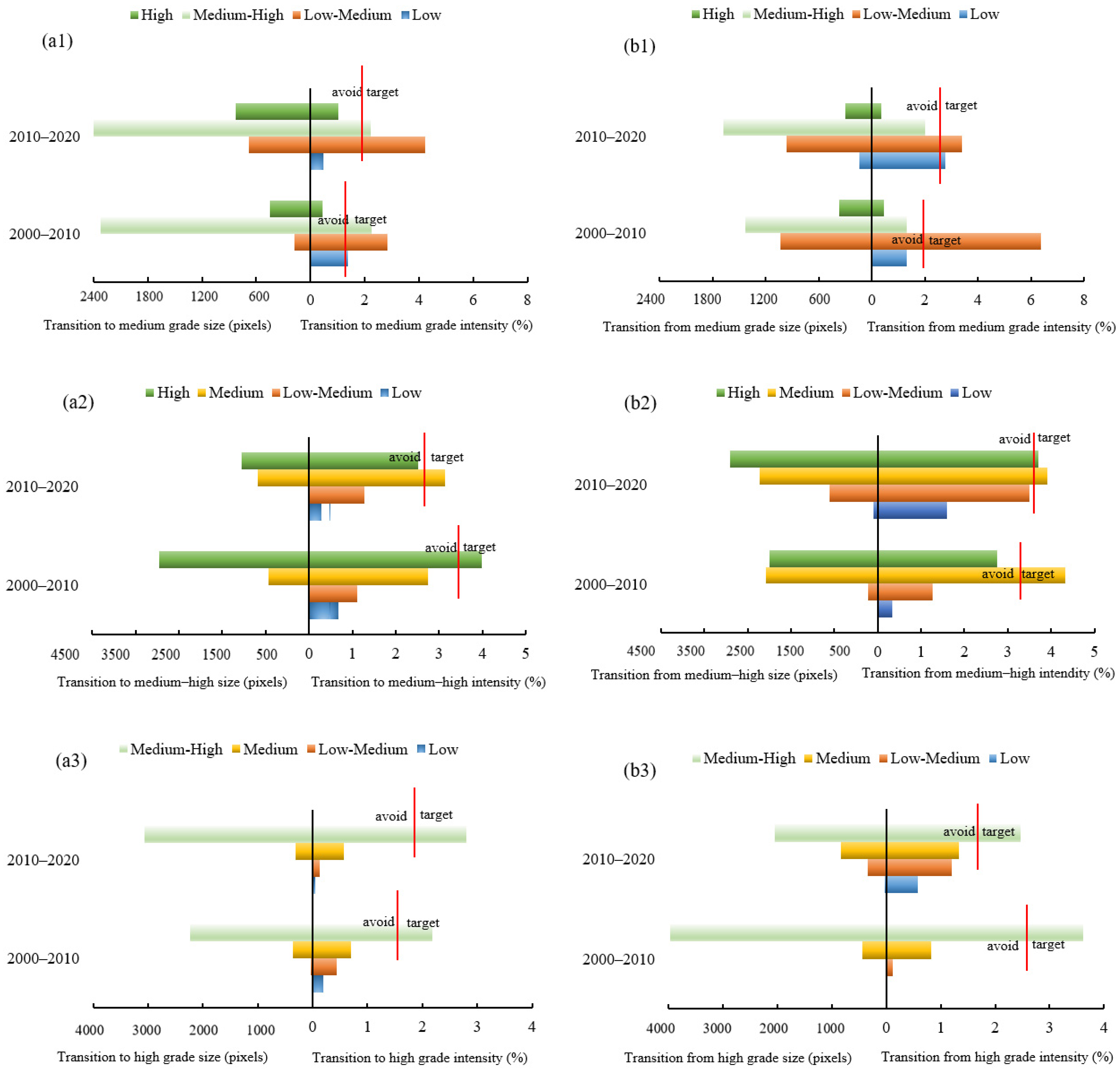
Considering the importance of vegetation coverage for carbon storage, soil conservation, and flood regulation, improving the vegetation condition is crucial. Therefore, in the transition intensity analysis, we mainly focused on transitions among the medium, medium–high, and high NDVI areas. To clarify the transition patterns among each NDVI grade, a transition level analysis was conducted, addressing the question, “Which grade was dominant in the transition process among the different grades of NDVI?” (Figure 10). Figure 10(a1,b1) show the transition to and from medium NDVI areas, from which we inferred that most of the largest transitions are from low–medium and medium–high NDVI areas in terms of size. The transition intensity indicated that the gain of medium NDVI areas targets low–medium and medium–high NDVI areas during the two periods. The transitions from medium NDVI areas were also primarily low–medium NDVI areas, indicating that mutual transitions between medium and low–medium NDVI areas were relatively frequent during the study period.
Similarly to those of the trends observed in the gain and loss of medium NDVI areas shown in Figure 10(a2), Figure 10(b2) shows the transition intensity for medium–high NDVI area gain and loss. Medium–high NDVIs lose more to medium and high NDVI areas than those to other NDVI grades during the two time periods because the gains of medium and high NDVIs target medium–high NDVI areas, whereas those of other NDVI grades avoid medium–high NDVI areas. Figure 10(a3,b3) show the transition intensity for the gain and loss of high NDVI areas. The high NDVI areas were mainly transferred to medium–high NDVI areas, and also mainly from medium–high NDVI areas.
To reveal the transition pattern for each NDVI grade, the dominant conversion forms are summarized in Table 3. We infer from the table that, in 2000–2010, low NDVI areas decreased and were mainly caused by the transition to low–medium NDVI areas; in 2010–2020, areas with low NDVI grades increased, which was the result of conversions from low–medium and medium NDVI areas. Low–medium NDVI areas increased during the two time periods and were mainly dominated by the transitions of low and medium NDVIs. Medium NDVI areas were mainly transferred from low–medium and medium–high NDVI areas, which caused an increase during the two time intervals. The medium–high NDVI areas declined in 2000–2010 and 2010–2020, resulting in the transformation of medium and high NDVI areas. High NDVI areas came from medium–high NDVI areas during 2000–2010, and were then transferred to medium–high and medium NDVI areas during 2010–2020.

3.4. Spatial Distribution Characteristic in DLB

Moran’s I value for vegetation coverage in 2000, 2010, and 2020 was 0.2264, 0.2003, and 0.2127 (where the z scores were all over 35), respectively, which indicated that the vegetation coverage is positively correlated in space and agglomerated. The overall cluster tendency decreased slightly from 2000 to 2020. From the LISA map (Figure 11), it can be seen that the spatial outliers, including the High–Low outlier and Low–High outlier, were not easily discernible, while the HH cluster and LL cluster covered the greater part of the area. From 2000 to 2020, the DLB mainly exhibited three types of non-significant HH clusters and LL clusters. The HL outlier only occurred in 2000, scattered on the northern DLB. Compared to 2000, Moran’s I value in 2020 decreased to 0.2127, implying that the spatial agglomeration of vegetation coverage was of less significance than in 2000. The spatial autocorrelation from 2000 to 2020 expressed an analogous distribution, where the HH areas were mainly distributed in the western mountain area of the DLB, and the LL areas were concentrated in the southern part of the DLB, with a tendency of extending to the northern wetland of the DLB.

3.5. Influencing Factors of NDVI Spatial Variations

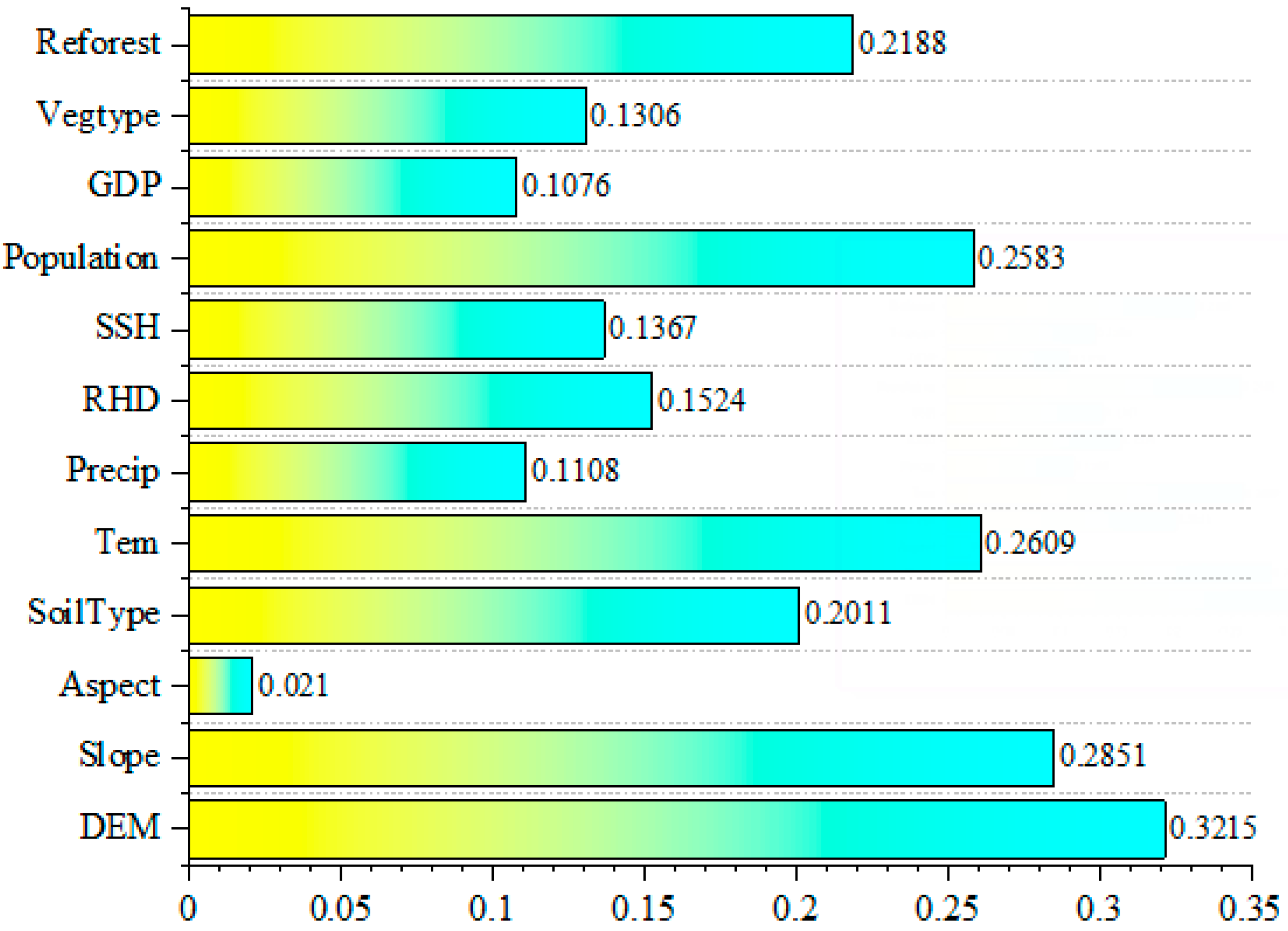
Factor detection was utilized to explore the explanatory power of various factors on the spatial differentiation of the NDVI distribution in the DLB, and the results are shown in Figure 12. The p value of all indicators is less than 0.05, which implied that the explanatory power for each indicator was significant to the spatial variation in vegetation coverage. Among these impact factors, the DEM had > 30% explanatory power (32.15%). Therefore, the DEM emerged as the primary impact factor of the spatial variation in vegetation coverage. The three factors with the highest explanatory power were DEM, slope, and population density. The factors were ranked from high- to low-power as follows: DEM > slope > population density > annual average temperature > reforested area > soil type > relative humidity degree (RHD) > vegetation type > sunshine hours (SSH) > GDP > annual precipitation > aspect. The slope, population density, annual average temperature, and reforested area, possessing q-values ranging from 0.2 to 0.3, served as secondary impact factors on spatial variation in vegetation coverage. Conversely, aspect, which had a q-value below 0.1, exerted a lower impact on vegetation coverage distribution. Overall, topographic factors were the dominant factors influencing the spatial distribution of vegetation coverage in the DLB, while anthropogenic activity also significantly affected the vegetation coverage distribution. Human activities have both a positive and negative impact on vegetation succession. Ecological protection strategies such as the Grain to Green policy converted farmland with slopes greater than 25 degrees into forest land, which led to the conversion from farmland to forest. Contrarily, rapid urbanization due to a high population density led to a conversion from vegetation cover to construction land, which caused a reduction in vegetation coverage [19].
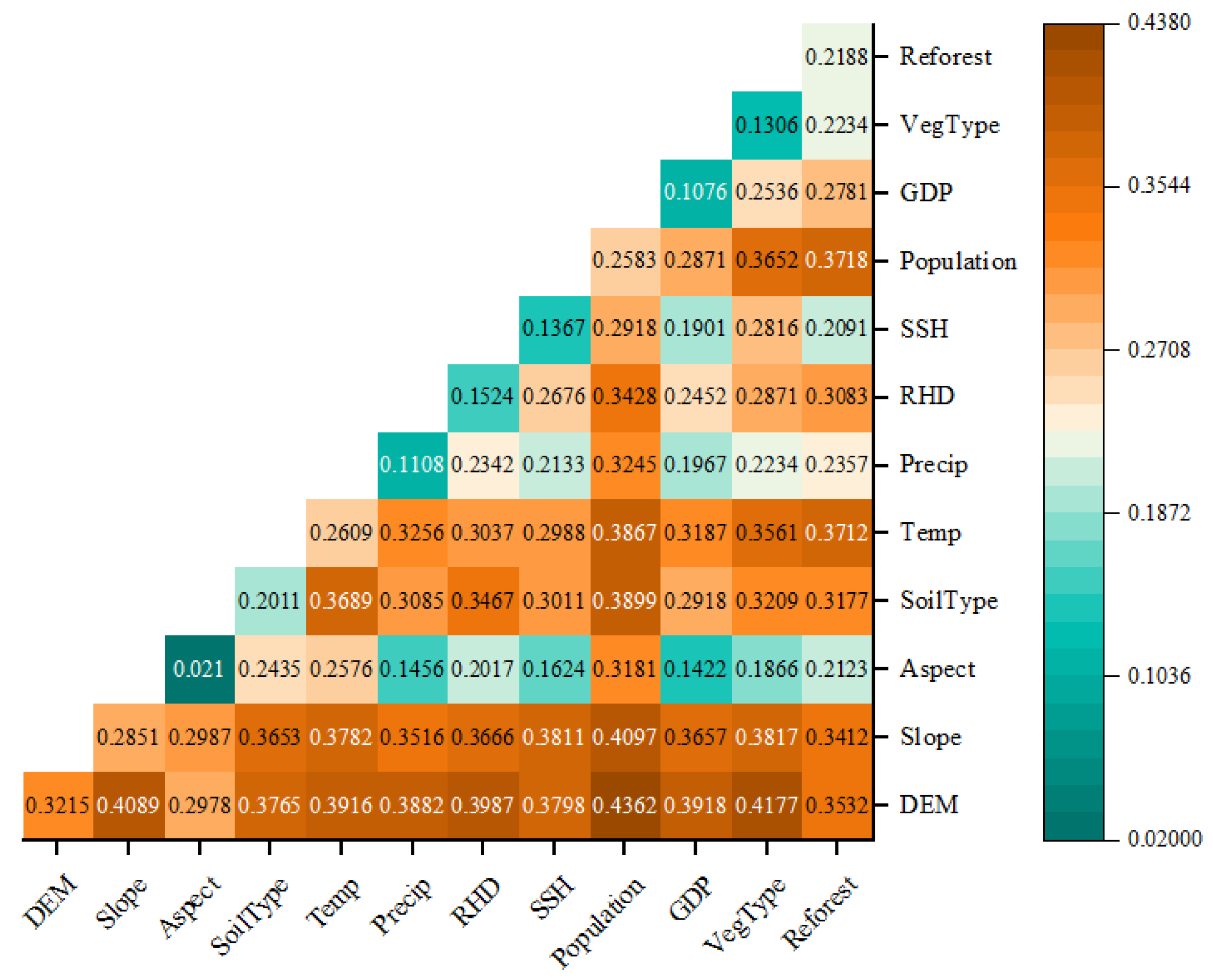
We further analyzed the interactions between each factor by employing an interaction detector for the DLB (Figure 13). The results revealed that the interaction q-value of each pair of factors was greater than that of a single factor, indicating that a dual-factor or non-linear enhancement occurred between any two factors. Specifically, the strongest interaction effects were DEM ∩ population density (0.4362) > DEM ∩ vegetation type (0.4177) > slope ∩ population density (0.4097) > DEM ∩ slope (0.4089) > DEM ∩ RHD (0.3987).
These findings demonstrate that the spatial distribution of vegetation coverage is associated with multiple interacting factors, with significant interactive and strengthening effects. The q-value for the independent aspect factor was 0.021, whereas the interactive explanatory power of aspect and population density was 0.3181, which implies that aspect did not affect vegetation coverage distribution unless it interacted with other influencing factors. Therefore, future decisions on vegetation protection should comprehensively evaluate the interactions between multiple dimensions.

3.6. Relationship Between Climate Change and NDVI Change

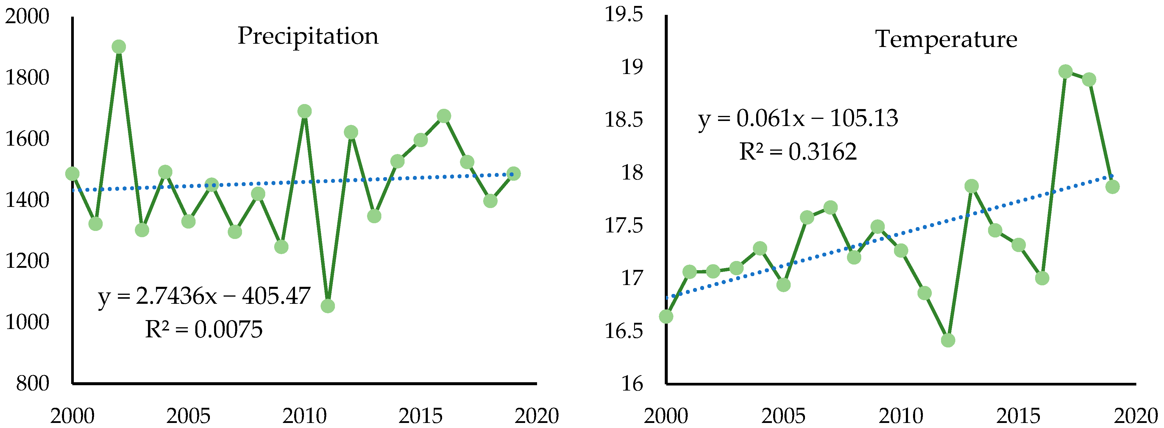
As shown in Figure 14, from 2000 to 2020, the annual precipitation and annual average temperature showed an increasing trend. The rate of temperature increase (r2 = 0.316, p < 0.01) is significantly higher than that of precipitation (r2 = 0.008). Annual precipitation and annual average temperature increased by 2.74 mm and 0.061 °C per year, respectively, which indicated that the DLB became drier and warmer.
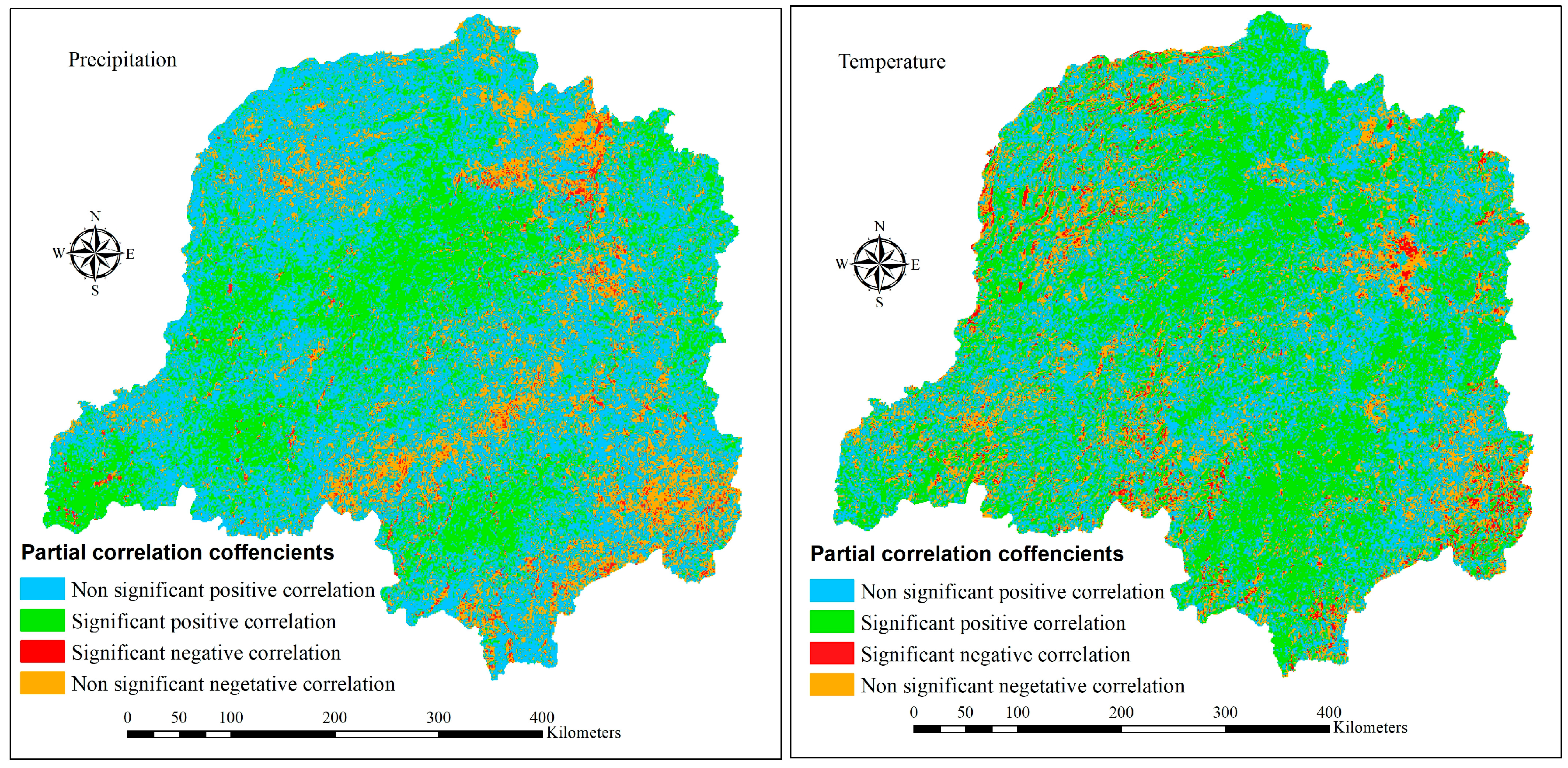
To clarify the response of the NDVI to precipitation and temperature changes at the pixel scale in the DLB, the partial correlation coefficient of the NDVI with precipitation and temperature over 21 years was calculated through a partial correlation analysis (Figure 12). The results showed that the temperature and precipitation were positively correlated with NDVI changes, and the partial correlation coefficients were 0.636 (p < 0.05) and 0.328 (p < 0.05), respectively. The partial correlation coefficient between NDVI and temperature was greater than that between NDVI and precipitation, indicating that temperature was the dominant climatic variable influencing the vegetation change in the DLB from 2000 to 2020.
Additionally, the spatial distributions of the partial correlation coefficients between NDVI with precipitation and temperature are displayed in Figure 15. NDVI change expressed a positive correlation with temperature, and areas with a non-significant positive correlation and significant positive correlation between the NDVI and temperature accounted for about 44.95% and 36.86% of the total area, respectively (Table 4). Areas showed a negative correlation between the NDVI and temperature, accounting only for 18.19%, which was scattered in the DLB. Generally, the NDVI had a positive response to temperature change in the DLB during the last 21 years, which showed that the changes in temperature positively impacted the vegetation coverage change from 2000 to 2020. The precipitation had a significant positive correlation with NDVI changes in the central and west part of the DLB, accounting for ~28.17% of the total study area. The area with a negative correlation between the precipitation and vegetation coverage accounted only for 19.6% and was mainly distributed in the east and north of the DLB. Summarily, the change in precipitation positively impacted the vegetation coverage change in the DLB from 2000 to 2020.

4. Discussion

4.1. Spatial and Temporal Change in NDVI

We analyzed the spatial and temporal dynamics of vegetation coverage in the DLB over the past 20 years using the NDVI derived from MODIS vegetation products. The NDVI inter-annual dynamic curve (Figure 4) shows that the NDVI increased at a rate of 0.37% per year from 2000 to 2020 and passed the significance test at a confidence level of 0.95 (Z > 1.96). This greening trend is consistent with that of the results of earlier research conducted at various spatial scales, including studies of the Yangtze River Basin [8,16,44,52,53], the Three Gorges Reservoir Region [14], and Dongting Lake [54]. However, the increasing trend was accompanied by fluctuations and distinct stage characteristics, which can be found from the Mann–Kendall mutation test of the average annual NDVI; the UF(k) curve showed an upward fluctuation from 2000 to 2020. The intersection of UF and UB occurred in 2010, representing the NDVI transformation from a slow to a significant upward trend. Vegetation coverage from 2008 to 2010 showed a slightly declining trend, which may have been a result of the implementation of ecological projects. As demonstrated by Zhang et al. [55], the first round of afforestation was completed during this period, and the emergence of returning farmlands to forests destroyed the natural ecological environment. Contrastingly, vegetation growth was spatially heterogeneous, which is consistent with earlier conclusions [8,33,44]. The eastern and western mountainous parts of the DLB showed a significant increasing trend, likely due to the influence of climatic and topographical factors. However, the northern part of the DLB exhibited a degradation trend. It is well established that the northern region of the DLB is dominated by wetland; thus, the vegetation growth is closely related to the water level [20].

4.2. Response of Vegetation Coverage Change on Climate Change

Climate change was considered to be a key factor of vegetation dynamics [7,14,22]. A thorough grasp of the climate–NDVI response mechanisms is essential to predict vegetation dynamics and inform effective ecological restoration strategies. Previous studies reported that vegetation coverage in the Yangtze River Basin was significantly influenced by climatic factors [7,16]. Zhang et al. [56] clarified that meteorological factors are linearly related to the NDVI in the Yangtze River Basin and that temperature exerts a stronger influence on vegetation dynamics than that of precipitation. Zhang et al. [57] analyzed the driving forces of vegetation dynamics utilizing a partial correlation analysis and indicated that vegetation coverage change was mainly controlled by climatic factors such as temperature, precipitation, and solar radiation. Jian et al. [58] took the Yellow River Basin as a study area and demonstrated that vegetation coverage in the Yellow River Basin exhibited a strong positive relationship with both precipitation and temperature. Moreover, within the same scenario, the annual average temperature emerged as a dominant factor influencing vegetation coverage changes in the majority of the Yellow River Basin. Liang et al. [59] investigated vegetation coverage trends and their driving factors in the upper Yellow River, finding that vegetation coverage exhibited a greater sensitivity to temperature than to precipitation. However, some research reported that the vegetation coverage change was mainly affected by temperature and was less related to precipitation [60]. Our findings demonstrate that climate change was positively related to the vegetation coverage change, and temperature was the dominant climatic variable influencing vegetation dynamics, which is consistent with earlier studies. The change in temperature will directly affect vegetation transpiration and soil evaporation, which might alter the utilization efficiency of vegetation water and further influence vegetation growth. Although the precipitation change also had a positive influence on vegetation coverage, the impact is weaker than that of temperature. This might be because the annual precipitation in the humid DLB is generally sufficient for vegetation growth, but the seasonal distribution of precipitation also has a significant impact on vegetation coverage.

4.3. Research Limitations

The vegetation index, derived from remote sensing images, has been regarded as an effective indicator for identifying vegetation types and monitor vegetation growth, since it can reduce the impacts of radiative changes caused by atmospheric and topographical conditions on surface reflectance. Thus far, numerous studies have used the vegetation index to analyze vegetation coverage changes. In this research, considering data availability and processing, the NDVI was used to investigate the vegetation coverage change. Although it was proven that, in the Dongting Lake Basin, the NDVI is effective for studying vegetation coverage [14,19], it still has some limitations that should be considered. For instance, the NDVI reaches saturation and has a low sensitivity in highly vegetation-covered forest land, and cannot accurately investigate vegetation coverage changes caused by short-term extreme weather events [61]. Therefore, in future studies, multiple vegetation indices, including EVI and TSAVI, and multi-source vegetation products, including Landsat-derived NDVI and SPOT, should be comprehensively applied to quantitatively evaluate the vegetation coverage change and pursue the accuracy of vegetation coverage detection.
Intensity analysis investigates the gross magnitude of categorical changes and the relative intensity with which these changes occur across different vegetation levels, the activity or dormancy of each vegetation level, and transition mechanisms between different vegetation levels in each period. However, owing to its neglect of data uncertainty, inter-category overlap, and spatial distribution, this method needs a further spatial variation analysis. Therefore, further research needs to consider the spatial position in the analysis process so that not only the temporal change but also the spatial variation can be identified.
Here, the Geodetector model was applied to explore the key factors impacting the spatial variability of vegetation coverage, and a partial correlation analysis was employed to investigate the relationship between climate change and vegetation dynamics. However, due to the complex mutual interaction of anthropogenic factors and natural factors, the intrinsic correlation mechanism still requires further explanation and validation. Simultaneously, other factors such as policy were not considered here because these factors are difficult to quantify. Therefore, in future research, more robust alternatives, such as variance partitioning or the BFAST model, should be employed to consider a wide range of indicators for vegetation coverage change. Furthermore, the incorporation of quantified data on policy implementation (e.g., afforestation area, investment) would also help bridge the gap between statistical correlation and causal mechanisms, moving the research in line with the most advanced socio-ecological system analysis.

5. Conclusions

We analyzed the spatiotemporal dynamics of vegetation coverage over the DLB using the MOD13A1 dataset from 2000 to 2020. A Theil–Sen median analysis coupled with a Mann–Kendall test was employed to explore the temporal trends of NDVI change. An intensity analysis was used to investigate the spatial distribution characteristics of different NDVI levels across different time periods. Thereafter, the Geodetector model was used to detect the key influencing factors and their interaction relationships with each independent factor affecting spatial variations in vegetation coverage, and a partial correlation analysis was utilized to analyze the relationship between vegetation coverage change and climate change. The results are as follows:
(1)
Spatially, vegetation coverage in the DLB was maintained in good condition, with higher NDVI levels in the western and eastern regions and relatively lower coverage in the central and northern areas. Temporal trends showed that, from 2000 to 2020, the average annual NDVI showed a generally increasing trend, with fluctuations in 2010; areas with an upward NDVI trend accounted for 87.55% and were mainly distributed in the forest area.
(2)
The seasonal average NDVI showed different dynamic changes during the study period, and the NDVI in winter showed a more rapidly changing trend compared with those of the other three seasons. Abrupt changes in the NDVI in spring, summer, autumn, and winter occurred in 2003, 2006, 2000, and 2006, respectively.
(3)
Based on the intensity analysis, vegetation growth was primarily characterized by an increase in medium–high and low–medium vegetation from 2000 to 2020, whereas areas with high NDVI values experienced some decline. Contrastingly, 2010–2020 saw a dominant expansion of high NDVI vegetation accompanied by a reduction in low–medium and low NDVI vegetation.
(4)
According to the Geodetector results, topographic factors were the primary factors influencing vegetation coverage differentiation, and the DEM comprised a stronger explanatory power, with a q-value of 32.15%. Among the climatic factors, the annual average temperature exhibited a higher explanatory power (26.09%) for vegetation coverage, whereas precipitation demonstrated relatively weaker effects (11.08%). Furthermore, the interaction of each pair of factors strengthened the explanatory power of vegetation variations, among which the interaction between DEM and population density had the highest q-value. This implies that the interaction of DEM and population density exhibited great effects on the spatial distribution of the NDVI in the DBL.
(5)
Vegetation coverage change responded positively to climate changes in the DBL during 2000–2020. The partial correlation coefficient of the NDVI with temperature is greater than that with precipitation, which implies that the temperature is the main factor affecting vegetation coverage dynamics during the study period.
The research results can provide a scientific basis for the environmental protection of the Dongting Lake Basin and the implementation of climate change-related strategies. The findings can offer valuable insights for advancing sustainable forestry development. By dividing the DLB into different zones according to the vegetation coverage dynamics, areas where vegetation is seriously stressed or declining should strictly control the impact of human activities and be prioritized for policy and funding support. Considering that the vegetation coverage change was mainly affected by temperature, attention should therefore be focused on responding to changes in phenology and species migration caused by climate change when carrying out afforestation and other ecological restoration strategies.

Author Contributions

Conceptualization, T.Z.; methodology, T.Z.; formal analysis, T.Z. and Y.J.; writing—original draft preparation, T.Z.; data curation, T.Z. and Y.C.; writing—review and editing, T.Z. and P.C.; funding acquisition, T.Z., Y.J. and Y.C. All authors have read and agreed to the published version of the manuscript.

Funding

This research was funded by the Science and Technology Development Programme of Jilin Province (YDZJ202501ZYTS508); the Jilin Provincial Department of Education (JJKH20250951KJ); the National Natural Science Foundation of China (42307599); and the Science and Technology Development Plan Project of Siping City (2023075, 2023073).

Institutional Review Board Statement

Not applicable.

Informed Consent Statement

Not applicable.

Data Availability Statement

The original contributions presented in this study are included in the article. Further inquiries can be directed to the corresponding author.

Conflicts of Interest

The authors declare no conflicts of interest.

References

  1. Setiawan, Y.; Yoshino, K.; Prasetyo, L.B. Characterizing the dynamics change of vegetation cover on tropical forestlands using 250 m multi-temporal MODIS EVI. Int. J. Appl. Earth Obs. Geoinf. 2014, 26, 132–144. [Google Scholar] [CrossRef]
  2. Li, J.; Wang, J.; Zhang, J.; Zhang, J.; Kong, H. Dynamic changes of vegetation coverage in China-Myanmar economic corridor over the past 20 years. Int. J. Appl. Earth Obs. Geoinf. 2021, 102, 102378. [Google Scholar] [CrossRef]
  3. Lewis, S.L.; Lloyd, J.; Sitch, S.; Mitchard, E.T.A.; Laurance, W.F. Changing ecology of tropical forests: Evidence and drivers. Annu. Rev. Ecol. Evol. Syst. 2009, 40, 529–549. [Google Scholar] [CrossRef]
  4. Liu, Y.; Li, L.; Chen, X.; Zhang, R.; Yang, J. Temporal-spatial variations and influencing factors of vegetation cover in Xinjiang from 1982 to 2013 based on GIMMS-NDVI3g. Glob. Planet. Change 2018, 169, 145–155. [Google Scholar] [CrossRef]
  5. Piao, S.; Wang, X.; Ciais, P.; Zhu, B.; Wang, T.; Liu, J. Changes in satellite-derived vegetation growth trend in temperate and boreal Eurasia from 1982 to 2006. Glob. Change Biol. 2011, 17, 3228–3239. [Google Scholar] [CrossRef]
  6. Arneth, A.; Harrison, S.P.; Zaehle, S.; Tsigaridis, K.; Menon, S.; Bartlein, P.J.; Feichter, J.; Korhola, A.; Kulmala, M.O.D.; Schurgers, G.; et al. Terrestrial biogeochemical feedbacks in the climate system. Nat. Geosci. 2010, 3, 525–532. [Google Scholar] [CrossRef]
  7. Piao, S.; Yin, G.; Tan, J.; Cheng, L.; Huang, M.; Li, Y.; Liu, R.; Mao, J.; Myneni, R.B.; Peng, S.; et al. Detection and attribution of vegetation greening trend in China over the last 30 year. Glob. Change Biol. 2015, 21, 1601–1609. [Google Scholar] [CrossRef]
  8. Zhang, W.; Wang, L.; Xiang, F.; Qin, W.; Jiang, W. Vegetation dynamics and the relations with climate change at multiple time scales in the Yangtze River and Yellow River Basin, China. Ecol. Indic. 2020, 110, 105892. [Google Scholar] [CrossRef]
  9. Bai, Y. Analysis of vegetation dynamics in the Qinling-Daba Mountains region from MODIS time series data. Ecol. Indic. 2021, 129, 108029. [Google Scholar] [CrossRef]
  10. Stow, D.A.; Hope, A.; Mcguire, D.; Verbyla, D.; Gamon, J.; Huemmrich, F.; Houston, S.; Racine, C.; Sturm, M.; Tape, K.; et al. Remote sensing of vegetation and land-cover change in Arctic Tundra Ecosystems. Remote Sens. Environ. 2004, 89, 281–308. [Google Scholar] [CrossRef]
  11. Tucker, C.J.; Newcomb, W.W.; Los, S.O.; Prince, S.D. Mean and inter-year variation of growing-season normalized difference vegetation index for the Sahel 1981–1989. Int. J. Remote Sens. 1991, 12, 1133–1135. [Google Scholar] [CrossRef]
  12. Pinzon, J.E.; Tucker, C.J. A Non-Stationary 1981–2012 AVHRR NDVI3g Time Series. Remote Sens. 2014, 6, 6929–6960. [Google Scholar] [CrossRef]
  13. Eastman, J.; Sangermano, F.; Machado, E.; Rogan, J.; Anyamba, A. Global trends in seasonality of Normalized Difference Vegetation Index (NDVI), 1982–2011. Remote Sens. 2013, 5, 4799–4818. [Google Scholar] [CrossRef]
  14. Wen, Z.F.; Wu, S.J.; Chen, J.L.; Lu, M.Q. NDVI indicated long-term interannual changes in vegetation activities and their responses to climatic and anthropogenic factors in the Three Gorges Reservoir Region, China. Sci. Total Environ. 2017, 574, 947–959. [Google Scholar] [CrossRef]
  15. Jiang, W.G.; Yuan, L.H.; Wang, W.J.; Cao, R.; Zhang, Y.F.; Shen, W.M. Spatio-temporal analysis of vegetation variation in the Yellow River Basin. Ecol. Indic. 2015, 51, 117–126. [Google Scholar] [CrossRef]
  16. Qu, S.; Wang, L.; Lin, A.; Zhu, H.; Yuan, M. What drives the vegetation restoration in Yangtze River basin, China: Climate change or anthropogenic factors? Ecol. Indic. 2018, 90, 438–450. [Google Scholar] [CrossRef]
  17. Cao, S. Why large-scale afforestation efforts in China have failed to solve the desertification problem. Environ. Sci. Technol. 2008, 42, 1826–1831. [Google Scholar]
  18. Piao, S.; Nan, H.; Huntingford, C.; Ciais, P.; Friedlingstein, P.; Sitch, S.; Peng, S.; Ahlström, A.; Canadell, J.G.; Cong, N.; et al. Evidence for a weakening relationship between interannual temperature variability and northern vegetation activity. Nat. Commun. 2014, 5, 5018. [Google Scholar] [CrossRef]
  19. Qi, S.Y.; Chen, S.D.; Long, X.; An, X.X.; Zhang, M. Quantitative contribution of climate change and anthropological activities to vegetation carbon storage in the Dongting Lake basin in the last two decades. Adv. Space Res. 2023, 71, 845–868. [Google Scholar]
  20. Liu, Y.; Li, J.T.; Yan, D.D.; Chen, L.; Li, M.; Luan, Z.Q. Typical vegetation dynamic and hydrological changes of Dongting Lake wetland from 1985 to 2020. Ecohydrol. Hydrobiol. 2024, 24, 910–919. [Google Scholar] [CrossRef]
  21. Sun, Y.L.; Shan, M.; Pei, X.R.; Zhang, X.K.; Yang, Y.L. Assessment of the impacts of climate change and human activities on vegetation cover change in the Haihe River basin, China. Phys. Chem. Earth Parts A/B/C 2020, 115, 102834. [Google Scholar]
  22. Bao, Z.; Zhang, J.; Wang, G.; Guan, T.; Jin, J.; Liu, Y.; Li, M.; Ma, T. The sensitivity of vegetation cover to climate change in multiple climatic zones using machine learning algorithms. Ecol. Indic. 2021, 124, 107443. [Google Scholar] [CrossRef]
  23. Long, X.; Li, X.; Lin, H.; Zhang, M. Mapping the vegetation distribution and dynamics of a wetland using adaptive-stacking and Google Earth Engine based on multi-source remote sensing data. Int. J. Appl. Earth Obs. Geoinf. 2021, 102, 102453. [Google Scholar] [CrossRef]
  24. Zhu, S.J.; Feng, W.W.; Zou, B.; Ye, S.C. Spatial-temproal characteristics of 2000–2019 vegetation NPP of the Dongting Lake basin and their driving factors. Remote Sens. Nat. Resour. 2022, 34, 196–206. [Google Scholar]
  25. Yang, N.; Mo, W.B.; Zhang, X.; Luo, W.J.; Zhang, C.M.; Zhao, Y.L.; Ma, F.F. Analysis of vegetation spatio-temporal variation based on NDVI of east Dongting wetland over the past 30 years. J. Cent. South Univ. For. Technol. 2019, 39, 19–30. [Google Scholar]
  26. Wei, D.; Liu, S.; Wu, Y.; Feng, S.; Gao, H.; Qin, C.; Ren, D.; Tang, W.; Zhang, Y. Impacts of human activities and climate change on water and sediment evolution in four large subtropical river basins in China. Ecol. Indic. 2023, 155, 110958. [Google Scholar] [CrossRef]
  27. Guo, J.; Guan, H.; Zhang, X. Growing season NDVI variation in the Dongting lake watershed from 1982 to 2010 and the climatic and anthropogenic influences. Resour. Environ. Yangtze Basin 2015, 24, 1305–1314. [Google Scholar]
  28. Hu, W.; Li, G.; Gao, Z.; Jia, G.; Wang, Z.; Li, Y. Assessment of the impact of the Poplar Ecological Retreat Project on water conservation in the Dongting Lake wetland region using the InVEST model. Sci. Total Environ. 2020, 733, 139423. [Google Scholar]
  29. Yuan, B.; Fu, L.; Zou, Y.; Zhang, S.; Chen, X.; Li, F.; Deng, Z.; Xie, Y. Spatiotemporal change detection of ecological quality and the associated affecting factors in Dongting Lake Basin, based on RSEI. Clean. Prod. 2021, 302, 126995. [Google Scholar]
  30. Zou, Y.A.; Zhang, P.Y.; Zhang, S.Q.; Chen, X.S.; Li, F.; Deng, Z.M.; Yang, S.; Zhang, H.; Li, F.Y.; Xie, Y.H. Crucial sites and environmental variables for wintering migratory waterbird population distributions in the natural wetlands in East Dongting Lake, China. Sci. Total Environ. 2019, 655, 147–157. [Google Scholar] [CrossRef]
  31. Zhao, Y.; Feng, Q. Identifying the spatiotemporal pattern and driving factors of vegetation dynamics in Shaanxi Province, China. Geocarto Int. 2022, 37, 17890–17916. [Google Scholar] [CrossRef]
  32. Zou, T.; Yoshino, K. Environmental vulnerability evaluation using a spatial principal components approach in the Daxing’anling region, China. Ecol. Indic. 2017, 78, 405–415. [Google Scholar] [CrossRef]
  33. Yuan, J.; Xu, Y.; Xiang, J.; Wu, L.; Wang, D. Spatiotemporal variation of vegetation coverage and its associated influence factor analysis in the Yangtze River Delta, eastern China. Environ. Sci. Pollut. Res. Int. 2019, 26, 32866–32879. [Google Scholar] [CrossRef]
  34. Tong, S.; Zhang, J.; Bao, Y.; Lai, Q.; Lian, X.; Li, N.; Bao, Y. Analyzing vegetation dynamic trend on the Mongolian Plateau based on the Hurst exponent and influencing factors from 1982–2013. J. Geogr. Sci 2018, 28, 595–610. [Google Scholar] [CrossRef]
  35. Liu, X.; Zhu, X.; Pan, Y.; Li, S.; Ma, Y.; Nie, J. Vegetation dynamics in Qinling-Daba Mountains in relation to climate factors between 2000 and 2014. J. Geogr. Sci. 2016, 26, 45–58. [Google Scholar] [CrossRef]
  36. Duo, A.; Zhao, W.; Qu, X.; Jing, R.; Xiong, K. Spatio-temporal variation of vegetation coverage and its response to climate change in North China plain in the last 33 years. Int. J. Appl. Earth Obs. Geoinf. 2016, 53, 103–117. [Google Scholar]
  37. Zhou, J.; Jia, L.; Menenti, M. Reconstruction of global MODIS NDVI time series: Performance of Harmonic ANalysis of Time Series (HANTS). Remote Sens. Environ. 2015, 163, 217–228. [Google Scholar] [CrossRef]
  38. Sen, P.K. Estimates of the regression coefficient based on Kendall’s Tau. J. Am. Stat. Assoc. 1968, 63, 1379–1389. [Google Scholar] [CrossRef]
  39. Yang, C.; Fu, M.; Feng, D.; Sun, Y.; Zhai, G. Spatiotemporal changes in vegetation cover and its influencing factors in the Loess Plateau of China based on the geographically weighted regression model. Forests 2021, 12, 673. [Google Scholar] [CrossRef]
  40. Kendall, M.G. Rank Correlation Methods, 4th ed.; Charles Grifin: London, UK, 1975. [Google Scholar]
  41. Geng, S.B.; Zhang, H.M.; Xie, F.; Li, L.H.; Yang, L. Vegetation dynamics under rapid urbanization in the Guangdong-Hong Kong- Macao Greater Bay area urban agglomeration during the past two decades. Remote Sens. 2022, 14, 3993. [Google Scholar] [CrossRef]
  42. Ullah, S.; You, Q.; Ullah, W.; Ali, A. Observed changes in precipitation in China-Pakistan economic corridor during 1980–2016. Atmos. Res. 2018, 210, 1–14. [Google Scholar] [CrossRef]
  43. Xu, J.H. Mathematical Methods in Contemporary Geography; Higher Education Press: Beijing, China, 2002; pp. 37–48. [Google Scholar]
  44. Qu, S.; Wang, L.; Lin, A.; Yu, D.; Yuan, M.; Li, C.A. Distinguishing the impacts of climate change and anthropogenic factors on vegetation dynamics in the Yangtze River Basin, China. Ecol. Indic. 2020, 108, 105724. [Google Scholar] [CrossRef]
  45. Aldwaik, S.Z.; Pontius, R.G. Intensity analysis to unify measurements of size and stationarity of land changes by interval, category, and transition. Landsc. Urban Plan. 2012, 106, 103–114. [Google Scholar] [CrossRef]
  46. Huang, B.Q.; Huang, J.L.; Pontius, R.G.; Tu, Z.S. Comparison of Intensity Analysis and the land use dynamic degrees to measure land changes outside versus inside the coastal zone of Longhai, China. Ecol. Indic. 2018, 89, 336–347. [Google Scholar] [CrossRef]
  47. Peng, W.F.; Kuang, T.T.; Tao, S. Quantifying influences of natural factors on vegetation NDVI changes based on geographical detector in Sichuan, western China. J. Clean. Prod. 2019, 233, 353–367. [Google Scholar] [CrossRef]
  48. Zou, T.H.; Chang, Y.X.; Chen, P.; Liu, J.F. Spatial-temporal variations of ecological vulnerability in Jilin Province (China), 2000 to 2018. Ecol. Indic. 2021, 133, 108429. [Google Scholar] [CrossRef]
  49. Cai, Y.T.; Liu, S.T.; Lin, H. Monitoring the vegetation dynamics in the Dongting Lake wetland from 2000 to 2019 using the BEAST algorithm based on dense Landsat time series. Appl. Sci 2020, 10, 4209. [Google Scholar] [CrossRef]
  50. Zhang, Y.; Zhang, L.Q.; Wang, J.Y.; Dong, G.C.; Wei, Y.L. Quantitative analysis of NDVI driving factors based on the geographical detector model in the Chengdu-Chongqing region, China. Ecol. Indic. 2023, 155, 110978. [Google Scholar] [CrossRef]
  51. Zeng, G.J.; Lai, X.; Liang, J.; Huang, L.; Li, X.D.; Long, Y.; Wu, H.P.; Yuan, Y.J. Water level response of east Dongting Lake wetland’s NDVI from 2000 to 2010. J. Hunan Univ. (Nat. Sci.) 2014, 41, 45–52. [Google Scholar]
  52. Yang, X.; Meng, F.; Fu, P.; Zhang, Y.; Liu, Y. Spatiotemporal change and driving factors of the Eco-Environment quality in the Yangtze River Basin from 2001 to 2019. Ecol. Indic. 2021, 131, 108214. [Google Scholar] [CrossRef]
  53. Cui, L.; Wang, L.; Qu, S.; Singh, R.P.; Lai, Z.; Yao, R. Spatiotemporal extremes of temperature and precipitation during 1960–2015 in the Yangtze River Basin (China) and impacts on vegetation dynamics. Theor. Appl. Climatol. 2018, 136, 675–692. [Google Scholar] [CrossRef]
  54. Zhang, M.; Lin, H.; Long, X.; Cai, Y. Analyzing the spatiotemporal pattern and driving factors of wetland vegetation changes using 2000–2019 time-series Landsat data. Sci. Total Environ. 2021, 780, 146615. [Google Scholar] [CrossRef] [PubMed]
  55. Zhang, Y.; Zhang, C.; Wang, Z.; Chen, Y.; Gang, C.; An, R.; Li, J. Vegetation dynamics and its driving forces from climate change and human activities in the Three-River Source Region, China from 1982 to 2012. Sci. Total Environ. 2016, 563–564, 210–220. [Google Scholar] [CrossRef] [PubMed]
  56. Zhang, L.; Chen, X.; Cai, X.; Habib, A.S. Spatial-temporal changes of NDVI and their relations with precipitation and temperature in Yangtze River Basin from 1981 to 2001. Geo-Spat. Inf. Sci. 2010, 13, 186–190. [Google Scholar] [CrossRef]
  57. Zhang, Y.; Shi, J.; Zhang, H.; Wu, B. Spatiotemporal patterns and driving forces of vegetation restoration and degradation in Dongting Lake wetland. Sci. Silvae Sin. 2024, 60, 1–13. [Google Scholar]
  58. Jian, S.Q.; Shi, S.J.; Cui, J.K.; Zhu, T.S.; Hu, C.H. Study on fractional vegetation cover dynamic in the Yellow River Basin, China from 1901 to 2100. Front. For. Glob. Change 2023, 6, 1157285. [Google Scholar] [CrossRef]
  59. Liang, Y.; Zhang, Z.Y.; Lu, L.; Cui, X.; Qian, J.K.; Zou, S.B.; Ma, X.L. Trend in satellite-observed vegetation cover and its drivers in the Gannan Plateau, Upper Reaches of the Yellow River, from 2000 to 2020. Remote Sens. 2022, 14, 3849. [Google Scholar] [CrossRef]
  60. Tao, S.; Peng, W.F.; Xiang, J.Y. Spatiotemporal variations and driving mechanisms of vegetation coverage in the Wumeng Mountainous Area, China. Ecol. Inform. 2022, 70, 101737. [Google Scholar] [CrossRef]
  61. Liu, L.; Yang, X.; Zhou, H.; Liu, S.; Zhou, L.; Li, X.; Yang, J.; Wu, J. Relationship of root zone soil moisture with solar-induced chlorophyll fluorescence and vegetation indices in winter wheat: A comparative study based on continuous ground-measurements. Ecol. Indic. 2018, 90, 9–17. [Google Scholar] [CrossRef]
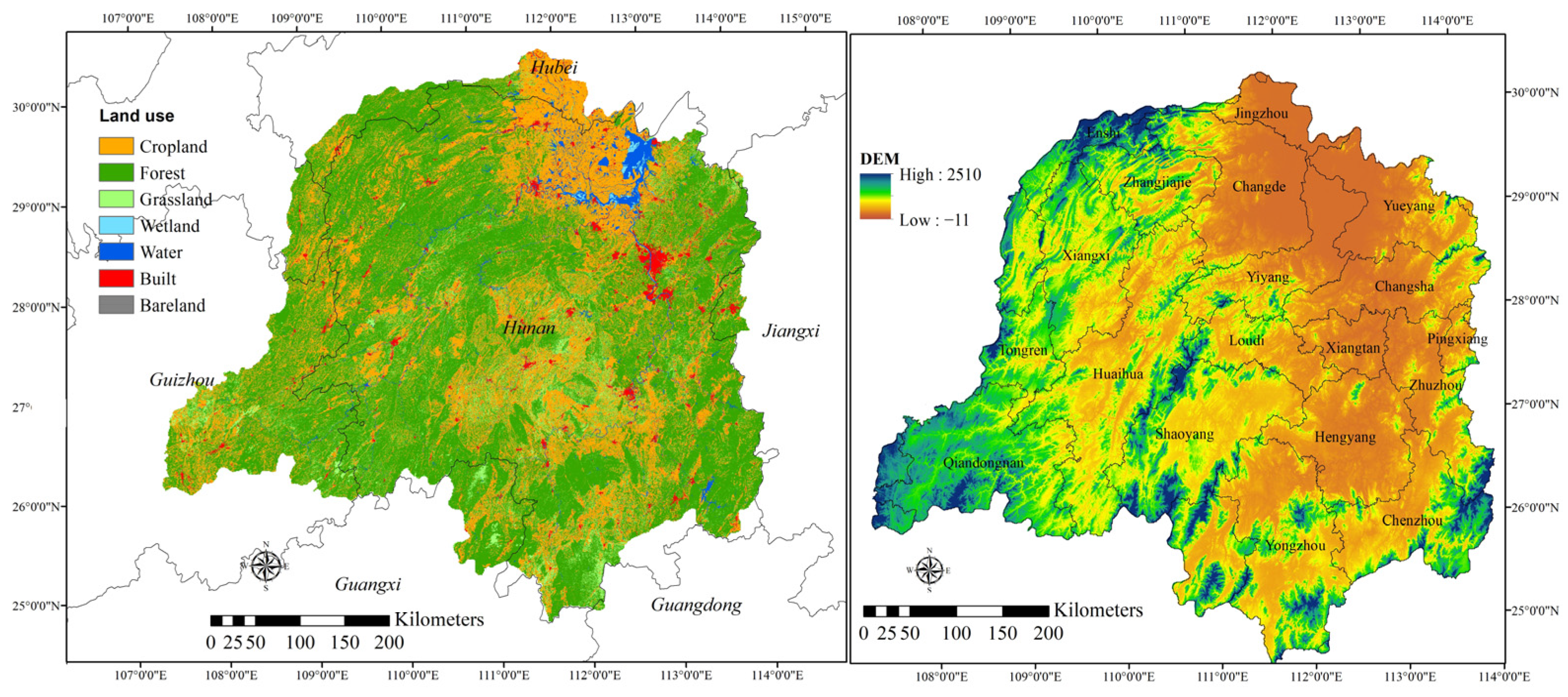
Figure 1. Location of the DLB. (Left) land use type; (right) elevation.
Sustainability 17 10543 g001
Figure 2. Spatial patterns of annual average NDVI. (a) Spatial distribution of annual average in DLB; (b) the area percentage of different annual average NDVI; (c) its elevation dependence in DLB.
Sustainability 17 10543 g002
Figure 3. Change trends (a) of NDVI and its fluctuations (b) in the DLB from 2000 to 2020.
Sustainability 17 10543 g003
Figure 4. Temporal variations in average NDVI in the DLB from 2000 to 2020. ((Left) inter-annual changes; (right) Mann–Kendall mutation detection).
Sustainability 17 10543 g004
Figure 5. Intra-annual variations in average NDVI in the DLB. ((Left) seasonal changes; (right) monthly changes).
Sustainability 17 10543 g005
Figure 6. Mann–Kendall mutation test of average monthly NDVI in spring (a), summer (b), autumn (c), and winter (d). The blue dash line represents the critical value at significance level of 0.05 (±1.96). UF(k) and UB(k) mean forward time series statistics and reserve sequence statistics, respectively.
Sustainability 17 10543 g006
Figure 7. Interval intensity for two time intervals: 2000–2010 and 2010–2020.
Sustainability 17 10543 g007
Figure 8. Category intensities for 2000 to 2010: (G) for gains and (L) for losses.
Sustainability 17 10543 g008
Figure 9. Category intensities for 2010–2020: (G) for gains and (L) for losses.
Sustainability 17 10543 g009
Figure 10. Transition intensity analysis between each NDVI level in two time intervals; (a) implies transfer-in and (b) represents transfer-out; (13) implies the level of different NDVI levels.
Sustainability 17 10543 g010
Figure 11. The cluster map of vegetation coverage in DLB. The gray region is the area without obvious clustering phenomena.
Sustainability 17 10543 g011
Figure 12. q-value of each factor of the factor detector.
Sustainability 17 10543 g012
Figure 13. Influence matrix diagram based on interaction detector.
Sustainability 17 10543 g013
Figure 14. Change trend of precipitation (left) and temperature (right) during 2000 to 2020 in DLB.
Sustainability 17 10543 g014
Figure 15. Spatial distribution of the partial correlation coefficients of NDVI with the annual precipitation (left) and annual average temperature (right) in DLB from 2000 to 2020.
Sustainability 17 10543 g015
Table 1. Transition matrix of NDVI categories in the DLB from two time intervals by area (km2): 2000–2010 (in bold); 2010–2020 (underlined).
NDVI CategoriesFinal Year of Time Interval
12345Initial TotalGross Loss
Initial year of time interval137740313969201008631
64314640254858215
23373194178570828063043110
188051626835206920916,15510,993
311410,31024,00914,345366252,44028,431
1375961222,77416,798303753,59630,822
428205523,20154,86722,411102,56247,695
794995024,41843,68930,694109,54565,856
52193446239,55655,06999,28244,213
2883439829320,43948,98381,44232,459
Final Total85816,15553,596109,54581,442
498028,30962,36083,02082,927
Gross Gain48112,96129,58754,67826,373
433723,14739,58639,33133,944
Table 2. Categories of interaction in Geodetector model.
Interaction TypesDescription
Non-linear enhancement q X 1 X 2 > q X 1 + q X 2
Independent q X 1 X 2 = q X 1 + q X 2
Bilinear enhancement q X 1 X 2 > M a x q X 1 , q X 2
Single-factor enhancement M i n q X 1 , q X 2 < q X 1 X 2 < M a x q X 1 , q X 2
Non-linear weaken q X 1 X 2 < M i n q X 1 , q X 2
Table 3. Conversion of dominant NDVI grades in the DLB during two time periods.
NDVI Grades2000–20102010–2020
Low NDVI (LN)(−) LMN(+) LMN, MN
Low–medium NDVI (LMN)(+) LN, MN(+) LN, MN, MHN
Medium NDVI (MN)(+) LMN, MHN, LN(+) LMN, MHN
Medium–high NDVI (MHN)(−) MN, HN(−) LMN, MN, HN
High NDVI (HN)(+) MHN(−) MHN, MN
Table 4. Area statistics of the correlation percentages in DLB from 2000 to 2020.
CorrelationNDVI and Temperature (%)NDVI and Precipitation (%)
Non-significant positive44.9552.23
Significant positive36.8628.17
Significant negative2.651.86
Non-significant negative15.5417.74
Disclaimer/Publisher’s Note: The statements, opinions and data contained in all publications are solely those of the individual author(s) and contributor(s) and not of MDPI and/or the editor(s). MDPI and/or the editor(s) disclaim responsibility for any injury to people or property resulting from any ideas, methods, instructions or products referred to in the content.