Fare Elasticity of Passengers in Mountainous Urban Rail Transit Considering Station Heterogeneity

Abstract

Promoting sustainable mobility and socio-economic sustainability through demand management is critical for mountainous urban rail systems. This study investigates urban rail transit in mountainous cities, focusing on how passenger travel behavior responds to time-based pricing policies across different station types, with the aim of informing differentiated fare policy design. Using Chongqing—a city with pronounced mountainous terrain—as a case study, we classified stations into 12 categories based on 11 indicators, including road slope, bus transfer density, average housing price, and peak-hour train crowding within a 500 m radius. This classification was then combined with questionnaire data to quantify fare elasticity of departure time. The results show that high-value bus-transfer congested stations are concentrated in central urban clusters with dense bus networks, mitigating terrain constraints and encouraging active travel. In contrast, low-value pedestrian-transfer comfort-oriented stations are predominantly located on the urban periphery, where sparse road networks and steep terrain exert greater influence. Low-value pedestrian-transfer congested stations exhibit the highest fare elasticity across all periods, indicating greater sensitivity to fare changes, while high-value bus-transfer comfort-oriented stations demonstrate the lowest elasticity, with passengers more likely to maintain existing travel patterns. Multiple linear regression identifies six significant determinants of fare elasticity, including section-level passenger crowding, average housing price, and bus route density. Sensitivity analysis using multinomial logistic regression further reveals that increasing bus route availability enhances the stability of low-value balanced-transfer comfort-oriented stations, whereas improving walkability can shift stations toward pedestrian-transfer types. By tailoring time-of-day pricing to station heterogeneity, policymakers can achieve equitable and environmentally friendly demand management, enhance operational efficiency and support sustainable urban development in mountainous regions.

1. Introduction

Rail transit dominates public transport in many major cities worldwide. As of 2024, the Tokyo Metro system [1] records a daily passenger volume of 6.84 million, with Ikebukuro Station [2] handling approximately 518,000 boarding passengers per day. Similarly, the New York City Subway [3] recorded an average weekday ridership of 3.40 million in 2024, with its busiest station complex, Times Square-42nd Street/Port Authority Bus Terminal, serving around 57.74 million passengers annually.

In Europe [4], major metro hubs such as Gare Saint-Lazare (33.12 million annual passengers) and Gare du Nord (34.50 million annual passengers) also exhibit substantial demand. These figures highlight the common challenges faced by metropolitan rail transit systems worldwide, including overcrowding during peak hours and underutilization of capacity during off-peak periods. Time-of-day pricing is a traffic demand management strategy that uses price incentives to redistribute passenger flows temporally, thereby helping to alleviate congestion [5]. Several transit systems have piloted time-differentiated fare policies with measurable success. For example, Melbourne’s “Early Bird Ticket” offered free travel before 7:00 AM, resulting in about 23% of holders shifting their trips earlier [6,7]. In Singapore, a weekday pre-peak travel (before 7:45 AM) free fare policy introduced in 2013 led to roughly 7% of peak commuters altering their departure times [8]. Dozens of cities including New York and Paris have implemented various forms of differential pricing [9]. In China, only the Beijing subway and Hong Kong MTR have experimented with time-based fare discounts. In late 2015, Beijing’s subway piloted a 30% discount before 7:00 AM at 16 stations on the Batong and Changping lines [10]; by the end of 2016, this was expanded to 24 stations with a 50% discount [11]. Hong Kong’s MTR implemented a 25% off-peak discount at 29 stations [12]. These initiatives demonstrate increasing attention to time-of-day pricing as a tool for congestion management. Understanding how fare changes affect passenger behavior is thus critical for designing effective time-based pricing policies. From a sustainability perspective, these time-of-day pricing policies are not only a tool for congestion management, but also a means to enhance the socio-economic and environmental performance of urban rail systems. By promoting a temporal redistribution of demand on existing high-capacity, low-carbon infrastructure, they can improve capacity utilization, reduce the need for energy- and material-intensive infrastructure expansion, and support more reliable and attractive public transport services as a core component of sustainable urban mobility.

Mountainous-city rail transit differs from plain-area systems in station context. Stations in mountainous cities often exhibit distinctive spatial patterns—for example, central urban clusters with highly concentrated development, hilly terrain with winding roads and steep slopes, fewer bus routes, and higher reliance on shuttle services—all of which can affect passengers’ choices of departure time and feeder mode under time-of-day pricing. In research on travel behavior heterogeneity, studies have typically focused on differences between passenger types, with less attention to variations in station environments [13]. However, the surrounding road network, transfer facilities, and built environment of a station in a mountainous city can significantly influence passenger behavior. It is therefore necessary to investigate fare elasticity under a refined station typology for mountainous metro systems, to provide theoretical support and quantitative evidence for differentiated time-of-day pricing strategies.

Against this background, this study contributes to sustainability research and practice in three ways. First, by integrating terrain-sensitive accessibility indicators into a 12-type station classification for a mountainous rail network, it provides a quantitative tool to characterize spatial heterogeneity in transit service and to monitor accessibility outcomes at station level. Second, by estimating fare elasticity of departure time across station types and time periods, the study supplies empirical evidence on how different communities respond to time-of-day pricing, thereby informing more socially equitable and demand-responsive fare policies. Third, by linking fare elasticity to built-environment and congestion indicators through regression and multinomial logit models, the paper offers a reproducible framework that decision-makers can use to evaluate and refine differentiated pricing scenarios as part of integrated sustainable urban mobility strategies.

2. Literature Review

2.1. Station Classification in Rail Transit

Station classification studies commonly use criteria such as location context, passenger flow magnitude, and connectivity mode. For example, Korf [14] selected station node and open-space characteristics to classify stations into five levels. The classic node–place model proposed by Bertolini [15] conceptualized stations as combinations of transportation accessibility (“node”) and urban development potential (“place”), and has been widely adopted for typology analysis in Europe and Asia. Zemp [16] further operationalized this framework using cluster analysis, identifying station types such as balanced, node-stressed, and place-stressed based on a large Swiss dataset. Similar frameworks have been applied internationally—e.g., Schimek and Pang [17,18] showed that integrating service frequency, built environment, and ridership metrics enables meaningful classification of metro stations for policy and planning purposes.

With the rise of big data, some researchers incorporate multi-source data into station classification. For instance, Pang et al. [18] constructed an indicator system from built environment and socio-economic dimensions to classify Tianjin stations into three types (residential, employment, and balanced) and explored factors affecting ridership by type. Wang et al. [19] proposed a data-driven station classification considering both station attributes and first/last-mile connections. Building on the node–place tradition, recent work has further integrated the node–place model with explainable machine-learning techniques—for example, combining node–place indicators with Shapley additive explanations (SHAP) to develop interpretable metro ridership regression models that quantify the contribution of each factor at station level [20]. Around metro stations, graph-based deep learning approaches such as spatial–temporal adaptive graph convolutional networks (STAGCN) have been used to predict shared-bicycle demand, capturing fine-grained, multimodal interactions between station environments and surrounding bike flows [21]. These advances show that station typologies are increasingly linked to predictive and interpretable models of ridership and associated multimodal demand.

However, the transferability of these models to mountainous contexts remains limited. Studies in flat cities implicitly assume isotropic accessibility, which does not hold in steep terrain. Research from hilly and alpine cities—such as Lausanne and Geneva (Switzerland) and Grenoble (France)—demonstrates that elevation changes and fragmented road networks drastically reshape station catchments, pedestrian routes, and first/last-mile connectivity [22]. The frequently changing topography is one of the major obstacles to walkability in cities like Greater Sydney where surface elevations from mean-sea-level may vary from −4 m to 72 m within roughly one kilometer [23]. Gao et al. [24] pointed out that walking times in mountainous cities are generally longer than in plains, suggesting the need for new accessibility indicators. Hence, the proposed microscale walkability index will remain incomplete if it is not adjusted thoroughly by the impact of topography. These findings underscore the need to integrate topography-sensitive accessibility indicators—such as average slope, road growth coefficient—into mountain city station typologies to better meet residents’ travel needs and promote sustainable urban development.

2.2. Effect of Station Environment on Fare Elasticity

The physical and functional environment surrounding rail transit stations plays a crucial role in shaping fare elasticity—the sensitivity of ridership to price changes. Empirical research consistently shows that elasticity varies with urban form, accessibility, and congestion conditions. Holmgren’s [25] meta-analysis of over 100 global cases estimated an average short-run fare elasticity around −0.38, with substantial variation depending on city size, data source, and travel mode. In contrast, Schimek [17] found that in U.S. cities, systems with higher service frequency and multimodal integration displayed lower elasticities (−0.2 to −0.3), indicating that well-connected systems are more resilient to fare changes. Kholodov [26] used a natural experiment in Stockholm to estimate mode- and income-specific elasticities, finding stronger fare sensitivity among low-income passengers and those using feeder buses. Such analyses highlight the importance of micro-level data for capturing heterogeneity in fare response

Additionally, built environment and operational differences significantly impact fare elasticity. In Geneva [22], a 12.6% system-wide fare reduction between 2014 and 2015 led to a 10.6% increase in ridership, yielding an estimated elasticity of −0.84. Similar natural experiments in Stockholm and Paris [25] report elasticities near −0.3 to −0.5. These results indicate that systems with dense multimodal integration and compact land use tend to have lower absolute elasticities, while those with more dispersed access modes or severe peak-hour crowding exhibit higher sensitivity. Ridership congestion characteristics also modulate fare response. For instance, MTA data for New York City and Transport for London’s open datasets [27,28] reveal extreme heterogeneity in station-level volumes: several central stations exceed 10 million annual entries, while peripheral stations serve below 1 million. In dense, transit-dependent systems, congestion at peak hours reduces passengers’ tolerance for additional cost or time, thereby amplifying the behavioral impact of time-of-day or distance-based fare adjustments. Conversely, stations with strong feeder bus or pedestrian connectivity (as in Zurich or Grenoble) exhibit more stable demand even under fare variations, suggesting that enhanced accessibility can mitigate fare sensitivity.

Parallel to these empirical studies, a growing body of research employs advanced spatial–temporal modeling to predict and manage transit demand. Fine-grained spatial–temporal multilayer perceptron (MLP) models have been proposed for metro origin–destination prediction, enabling more accurate forecasting of OD flows at high temporal resolution [29]. Dynamic high-capacity ride-sharing models that incorporate subsequent information have been developed to reallocate demand in real time and coordinate with high-capacity transit services [30]. At the network scale, evolutionary game models have been applied to analyze the strategic behavior of different actors in air–rail intermodal transportation, revealing how pricing, service design, and information provision interact to shape user choices and system equilibrium [31]. Together, these studies illustrate how data-driven methods and multi-modal coordination can support demand management and pricing decisions across complex transport systems.

Overall, the literature demonstrates that the spatial heterogeneity of station environments produces significant variation in fare elasticity across regions and time periods. Integrating terrain and congestion indicators into the station classification framework, as performed in this study, extends previous models and improves understanding of passenger behavior in mountain-city metros. By coupling AFC data with survey-based elasticity estimation, the research provides a valuable empirical contribution to both international fare elasticity analysis and the theory of transit accessibility under complex topography.

3. Station Classification Methodology

3.1. Study Area

Chongqing’s urban rail transit network [32] comprises 13 operational lines with 305 stations and 522.54 km of operating track, serving a metropolitan population of over 30 million in the municipality. The city’s terrain is markedly hilly, with elevation often varying by approximately 100–200 m within a 1 km radius. Such topographic variation contributes to irregular street networks, steep pedestrian gradients, and constrained street cross-sections. Bus coverage is dense in central clusters but sparse in steep-slope neighborhoods where ‘alley buses’ and walking are dominant. These operational and morphological characteristics motivate the use of terrain-sensitive indicators in our station classification.

3.2. Indicator Selection

Taking Chongqing urban rail transit stations as the research object, a 500 m buffer zone is designated around each station to avoid insufficient coverage of 400 m and overlapping of adjacent stations of 800 m, which is particularly severe in dense mountainous networks [33,34,35]. Then, relevant indicators such as surrounding economic characteristics [15,16], bus connectivity [18,19], pedestrian accessibility, and train crowding levels for clustering analysis. From the perspective of network accessibility, bus and pedestrian connectivity indicators capture, to some extent, the influence of first- and last-mile mode choices. Given the mountainous context, we additionally incorporate average road slope and a road growth coefficient to reflect terrain variability and route indirectness. From the passenger perspective, train carriage crowding directly influences comfort and significantly shapes travel decisions and behavioral patterns. Furthermore, the economic conditions of the surrounding area are considered, as income levels are closely linked to passenger sensitivity under time-differentiated fare policies. Based on these considerations, the classification indicators and their calculation methods are defined as follows:

1. Bus connectivity. Using Baidu Map POI data, we compute, within 500 m of each station, the number of conventional bus routes, bus stops, alley bus routes, and average transfer distances. In total, 25,879 POI items are collected to evaluate the convenience of bus–metro transfers.

2. Pedestrian accessibility. Drawing on OpenStreetMap road network data and a 30 m Digital Elevation Model, we calculate the road growth coefficient and the average longitudinal slope within 500 m of each station. The road slope and growth coefficient capture the complexity of mountainous terrain and its impact on passenger travel behavior, thereby evaluating walkability and pedestrian feeder accessibility. In addition, to approximate the spatial distribution of passenger origins, we first identify its 500 m watershed for each station and then construct a set of surrogate origins by sampling the centroids of residential land polygons and residential type buildings extracted from OSM.

For each pair of start-station combinations within 500 m $(o,s)$, calculating the shortest reachable path length on the walking network described above $I$, and sampled the starting point from the DEM with the station elevation $H_o$, $H_s$. The average longitudinal slope of the horizontal path is as shown in Equation (1).

$$I={\displaystyle \frac{\left(H_s-H_o\right)}{L_t}}\times 100\%$$

(1)

where I denotes the average longitudinal slope; $H_s$ is the station elevation; $H_o$ is the passenger origin elevation; $L_t$ is the passenger travel distance.

The road growth coefficient describes the degree of path detour caused by the terrain and street network shape. For each origin–station pair $(o,s)$, let $L_s$ denote the Euclidean straight-line distance between the trip origin and the station centroid, and let $L_r$ denote the corresponding shortest-path walking distance along the pedestrian network., then the road growth coefficient at the path level is as shown in Equation (2).

$$C_r={\displaystyle \frac{L_r}{L_s}}$$

(2)

where $C_r$ is the road growth coefficient; $L_r$ is the actual walking distance; $L_s$ is the straight-line distance between trip origin and destination.

3. Economic level. From Baidu Map data, we extract average housing prices and the number of parking lots within 500 m of each station. The mean and standard deviation of housing prices are used to characterize the economic status and development intensity of the surrounding area.

4. Congestion Level. Automated fare collection (AFC) data are processed to couple OD flows with train operation schedules, enabling the calculation of sectional passenger volumes and cross-sectional flows. By comparing sectional passenger flows with train capacity (As shown in

Table 1. Rated train capacity and peak headways for Chongqing rail lines.

Line	Train Type	Train Consist	Rated Capacity (Passengers)	Peak Headway (min)
1	B-type metro	6-car	1468	4
2	Straddle monorail	6/8-car	962/1292	3
3	Straddle monorail	6/8-car	962/1292	3
4	A_s-type metro	6-car	1532	4
5	A_s-type metro	6-car	1532	4
6	B-type metro	6-car	1468	4
10	A_s-type metro	6-car	1532	4
Loop line	A_s-type metro	6-car	1532	5
Guobo line	B-type metro	6-car	1468	6

), we derive the average peak-hour congestion index, which represents passenger comfort. The index is calculated as shown in Equation (3) below.

$$\mathsf{\alpha }={\displaystyle \frac{{\mathrm{Q}}_h}{{\mathrm{Q}}_{\mathrm{y}}}}\times 100\%$$

(3)

where α denotes the average peak-hour congestion index; Q_h is the average sectional passenger flow during peak hours; Q_y is the line capacity.

In total, 11 indicators across four categories are selected as the basis for station clustering analysis. Since the indicators differ in scale, all variables are standardized prior to clustering.

Table 2. Standardized Results of Station Clustering Indicators.

Category	Indicator	Data Type	Standardized Range	Parameter
Bus Connectivity	Number of bus routes	Continuous	[−1.47, 3.66]	Rb
	Number of bus stops	Continuous	[−1.62, 2.88]	Sb
	Number of alley bus routes	Continuous	[−0.52, 5.00]	Ra
	Average transfer distance	Continuous	[−3.05, 3.05]	Dt
Pedestrian Accessibility	Road growth factor	Continuous	[−1.77, 2.57]	Cr
	Average longitudinal slope of roads	Continuous	[−3.83, 1.89]	I
Economic Level	Number of car parks	Continuous	[−0.80, 4.37]	Pa
	Average house price	Continuous	[−1.98, 3.03]	Hμ
	Standard deviation of house price	Continuous	[−1.34, 4.68]	Hσ
Congestion Level	Upstream peak-hour average congestion	Continuous	[−1.22, 2.75]	${\alpha }_u$
	Downstream peak-hour average congestion	Continuous	[−1.08, 3.68]	${\alpha }_d$

summarizes the standardized ranges of these clustering factors.

3.3. Determination of Cluster Number

The K-means clustering algorithm is an iterative method that continuously adjusts the positions of cluster centers to achieve an optimal classification outcome [36]. Given that the data in this study are continuous, the K-means algorithm is well suited for the clustering analysis. Prior to performing the clustering, it is necessary to determine the appropriate number of clusters. In this study, the “elbow method” is adopted to identify the optimal cluster number. Specifically, the sum of squared errors (SSE) is calculated under different cluster numbers, and the inflection point corresponding to the largest decline in Sse is selected as the optimal cluster number [37]. The SSE is computed as follows Equation (4):

$$Sse={\sum }_{i=1}^k{\sum }_{p\in C_i}{\left|P-m_i\right|}^2{\displaystyle \frac{Q_h}{Q_y}}\times 100\%$$

(4)

where k denotes the number of clusters, C_i represents the i-th subset of the clustering, P is a sample point within the subset, and m_i is the mean of all sample points in subset C_i.

3.4. Results Analysis

To achieve a more refined station classification that highlights the unique characteristics of mountainous cities, this study adopts a two-stage clustering strategy [38]. In the first stage, stations are clustered based on congestion and economic-level indicators. In the second stage, to further emphasize the influence of the mountainous urban road environment, stations are re-clustered using bus connectivity and pedestrian accessibility indicators. Through this two-stage process, 12 distinct station categories are obtained, as summarized in

Table 3. Station Classification Results.

Site Group	Site Type	Number of Stations	Typical Stations
1	High-value bus-transfer congested	13	Guanyinqiao
2	High-value pedestrian-transfer congested	10	Liugongli
3	High-value balanced-transfer congested	7	Longtousi
4	Low-value bus-transfer congested	7	Xuetangwan
5	Low-value pedestrian-transfer congested	2	Central Park
6	Low-value balanced-transfer congested	8	Shangxin Street
7	High-value bus-transfer comfort-oriented	9	Tongjiayuanzi
8	High-value pedestrian-transfer comfort-oriented	7	Haitangxi
9	High-value balanced-transfer comfort-oriented	25	Chongqing North Station
10	Low-value bus-transfer comfort-oriented	10	Tongyuanju
11	Low-value pedestrian-transfer comfort-oriented	24	Jinyu
12	Low-value balanced-transfer comfort-oriented	37	Yudong

. In addition, validity and robustness checks were conducted on the number of clusters, and it was found that 12 clusters were consistently supported as stable intervals, achieving a good balance between cohesion and separation.

Due to its topographical features, Chongqing’s stations have distinct environmental and functional characteristics: Jiefangbei, Guanyinqiao, and Nanping are representative high-value bus-transfer congested stations located in dense commercial cores with major interchange hubs; Daping, Liziba, and Shapingba exemplify high-value pedestrian-transfer congested stations where steep terrain limits bus access and pedestrian movements dominate; while Lianglukou, Hongqihegou, and Sigongli represent balanced-transfer congested stations integrating both bus and pedestrian flows in mixed-use areas. These examples reflect the diversity of Chongqing’s network and motivate the adoption of terrain-sensitive indicators in our station classification.

3.4.1. First-Stage Clustering (Congestion & Economic Level)

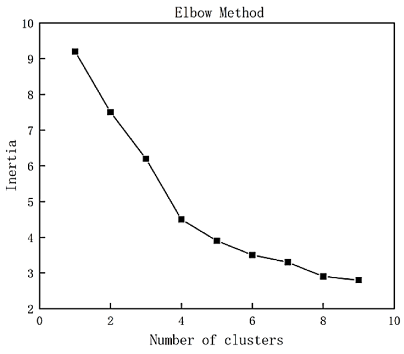
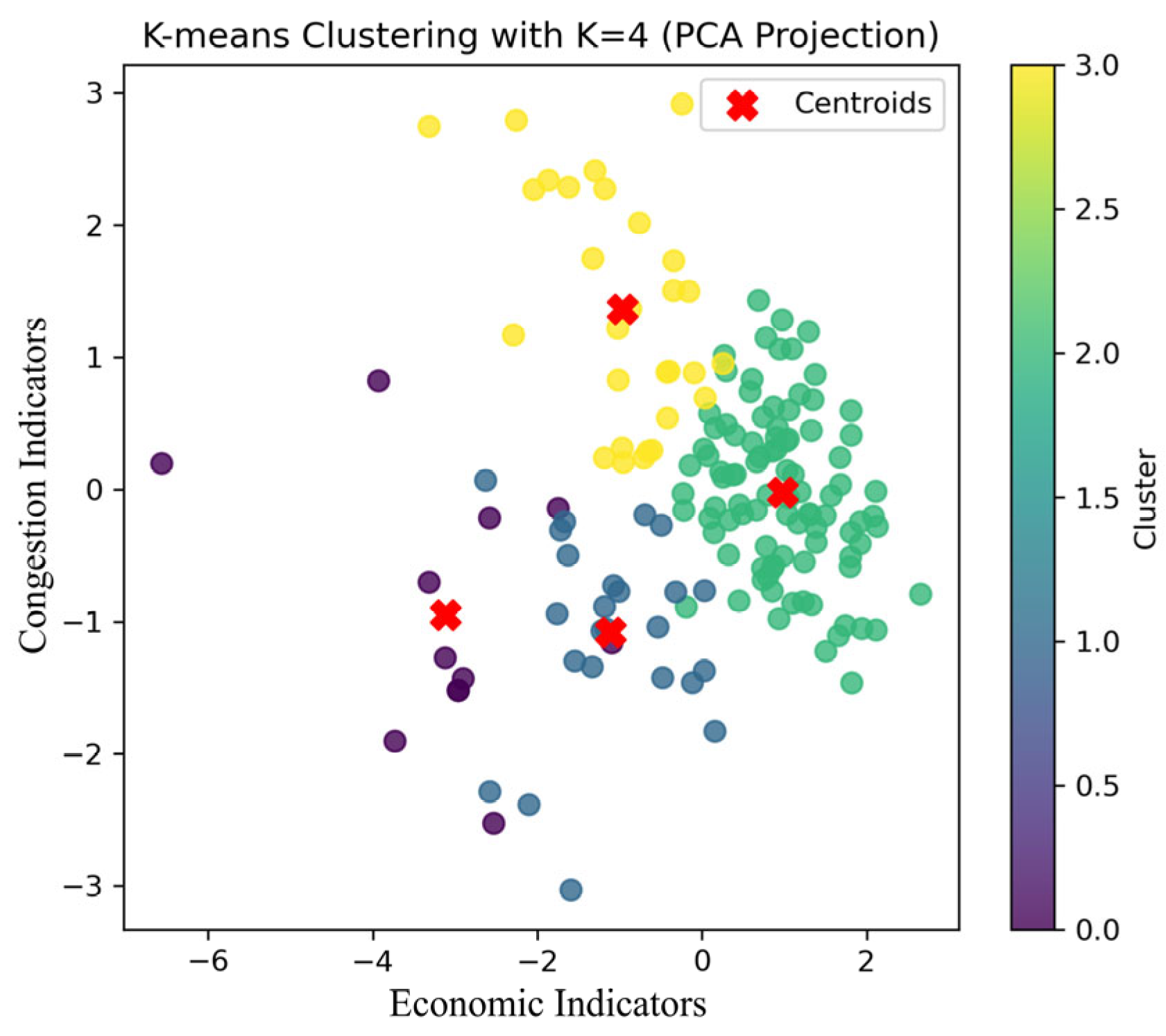
We processed AFC (Automatic Fare Collection) data to derive congestion indicators, which were combined with station-area economic characteristics for clustering analysis. The optimal number of clusters was determined using the elbow method. As shown in Figure 1, when the number of clusters K increases from 1 to 4, the distortion degree exhibits notable fluctuations; however, once K exceeds 4, the rate of decrease becomes much smaller. Therefore, the optimal cluster number was set to 4. Applying the K-means algorithm, the principal component analysis (PCA) visualization of the clustering results is presented in Figure 2, which depicts the sites in the first two principal component spaces, colored by four clusters.

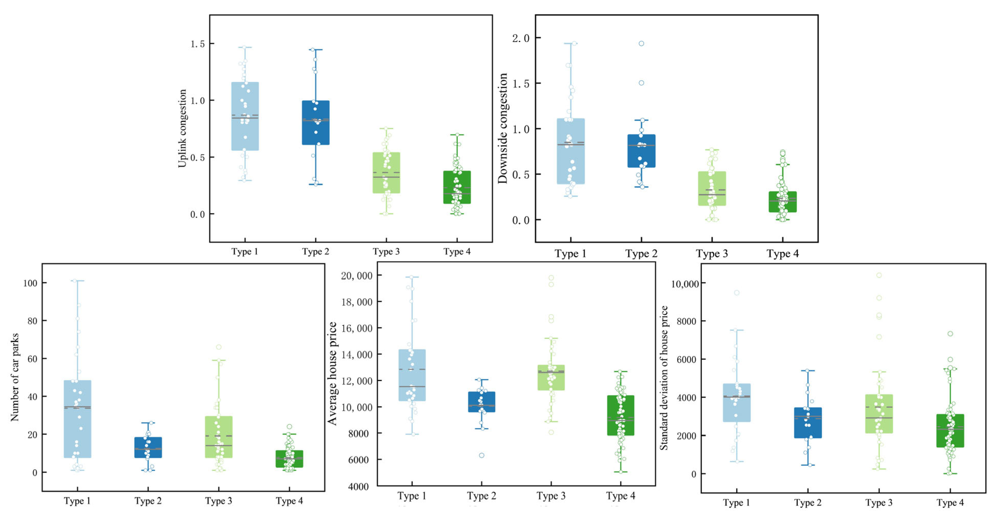
For the four station categories identified in the clustering results, Figure 3 presents boxplots of congestion and economic characteristics, which clearly illustrates the differences between clusters. For instance, high-value congested stations (Type 1) have the highest medians for housing prices and parking numbers, with relatively wide interquartile ranges. In contrast, low-value comfort-oriented stations (Type 4) show much lower median housing prices and narrower spreads.

• High-Value Congested Stations (Type 1): These stations exhibit significantly above-average surrounding housing prices and a higher number of parking facilities, coupled with high congestion levels. Typically located in central urban districts or economically developed areas, they feature strong parking demand, intensive land development, and dense concentrations of commercial and office jobs. The complex travel flows arise from diverse commuting, business, and public trips.
• Low-Value Congested Stations (Type 2): At least one travel direction experiences high congestion, while surrounding housing markets remain relatively stable with lower purchasing power. These stations are characterized by lower parking demand and weaker economic activity, and passengers are generally more sensitive to fare changes.
• High-Value Comfort-oriented Stations (Type 3): Stations in this category display relatively low congestion alongside higher average housing prices and greater variability, reflecting generally high but uneven income levels in surrounding areas.
• Low-Value Comfort-oriented Stations (Type 4): These stations show low congestion (comfortable riding conditions), combined with lower average housing prices and smaller variation. They typically have fewer parking facilities and are often located on the urban periphery or in developing districts, indicating lower surrounding income and weaker economic activity.

3.4.2. Second-Stage Clustering (Bus and Pedestrian Accessibility)

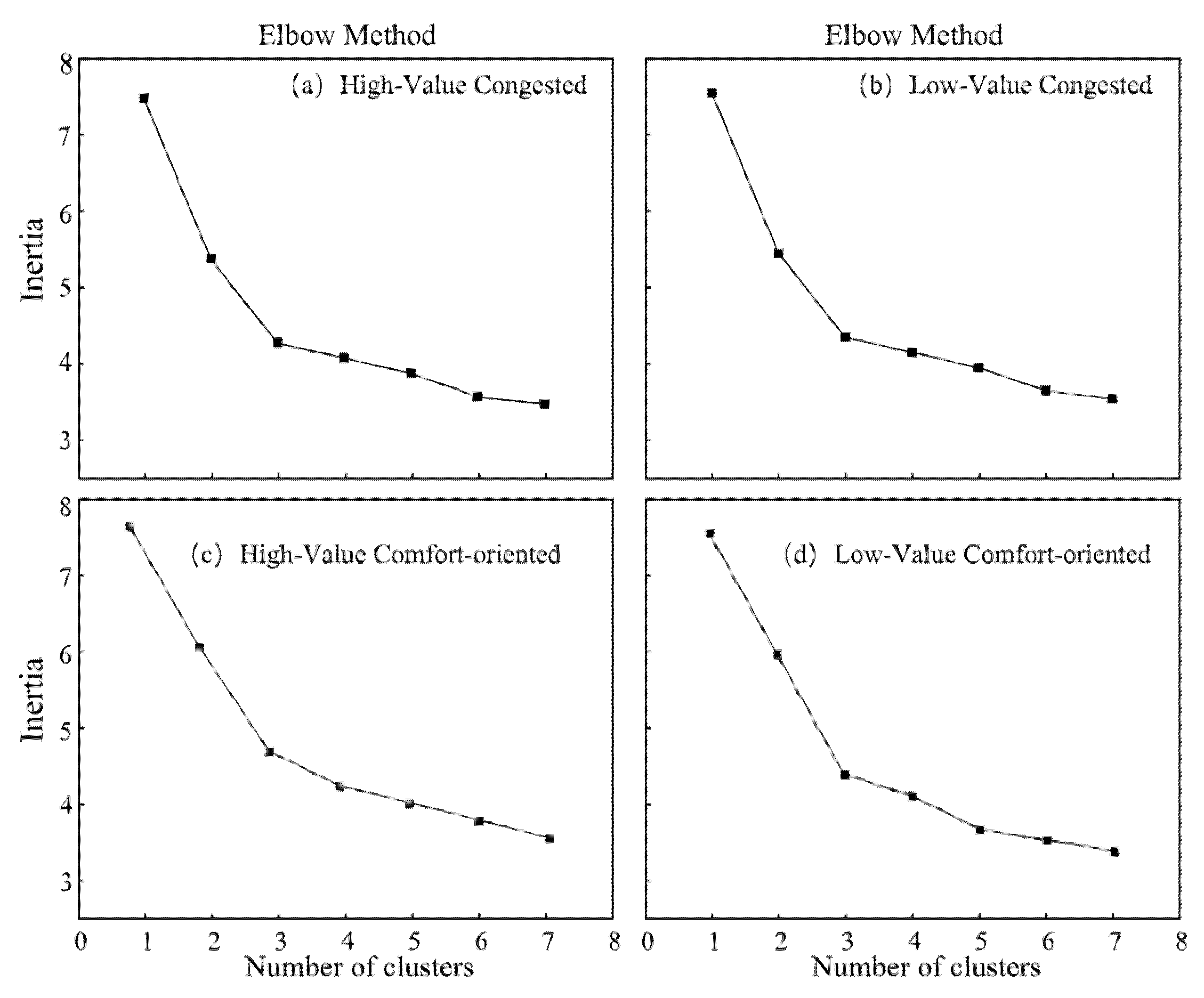
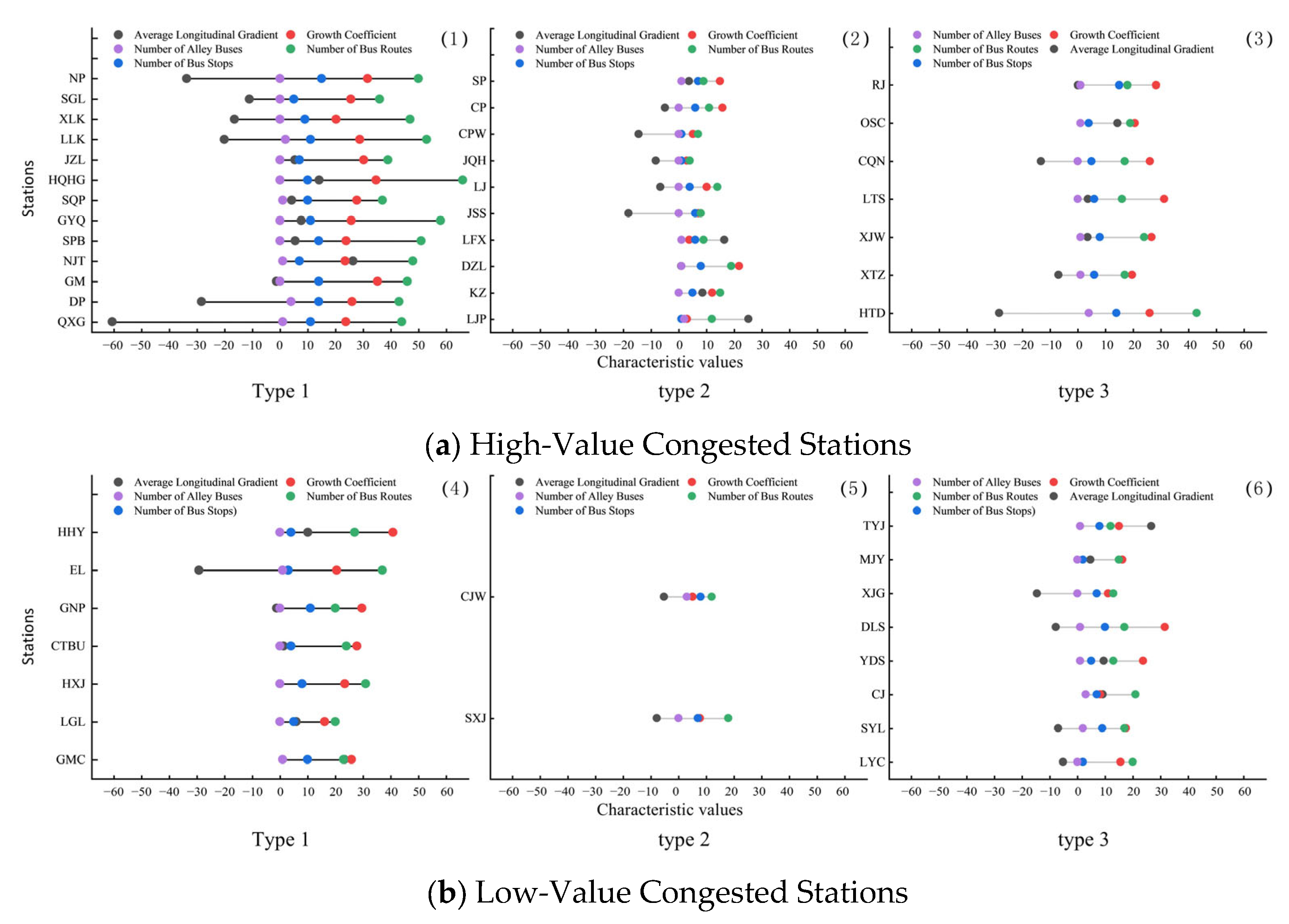
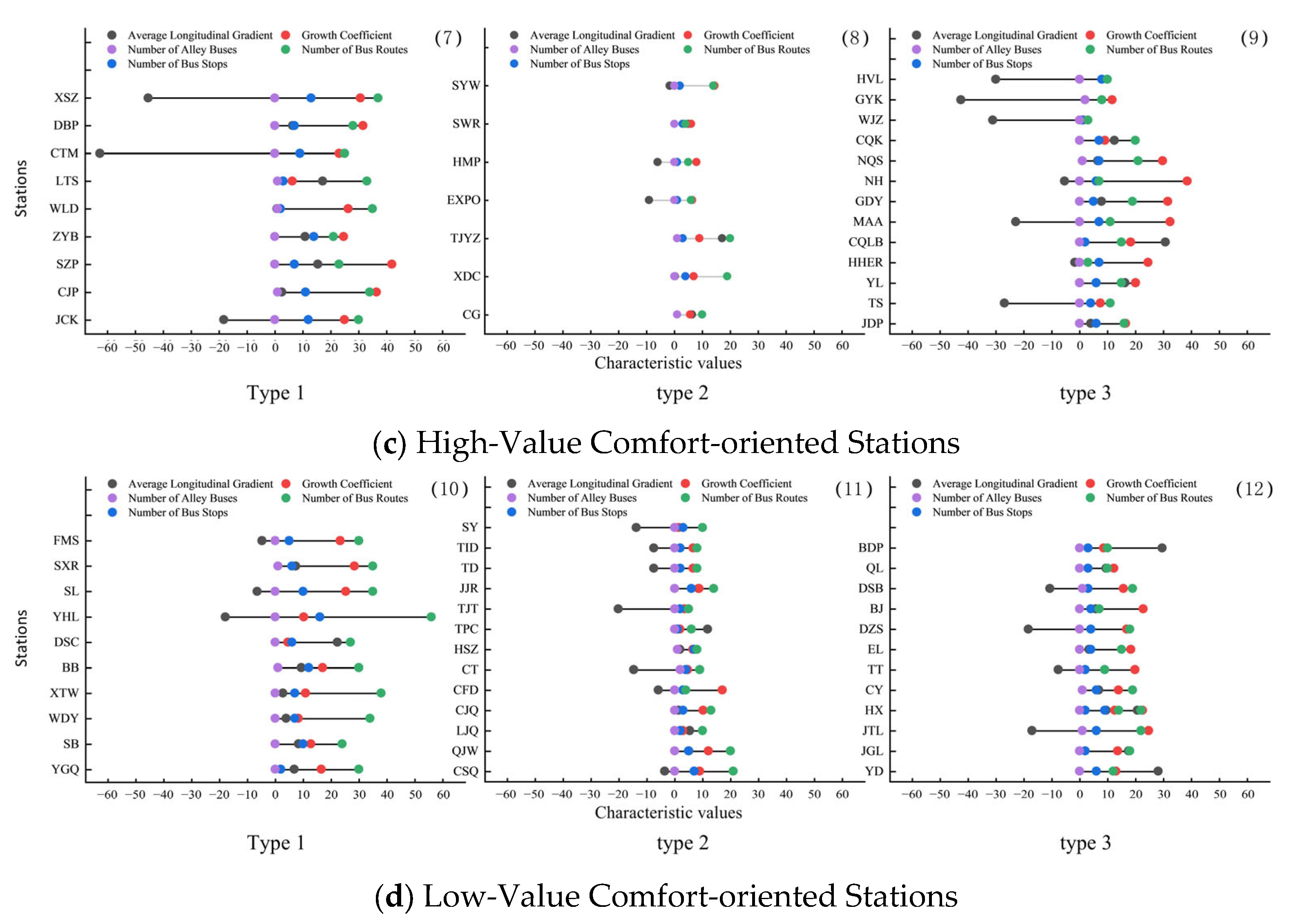
From Figure 4, it is evident that the distortion index for different station categories reaches its maximum at three clusters, after which the value declines substantially. Accordingly, the number of clusters selected for further analysis is set to three. Using the K-means algorithm, stations are subsequently subdivided, resulting in a total of twelve station categories. To further assess their characteristics, the pedestrian accessibility and transfer connectivity of each category were analyzed, with results presented in Figure 5, which compares transfer-related clusters within each original category. For example, in Figure 5a, the bus transfer subtype has the highest bus route density and very low slope, while the pedestrian transfer subtype has the smallest bus passage and relatively flat terrain. Similarly, Figure 5d shows that the balanced transfer station has intermediate values on both axes. Through the reading axis, people can see that the type of public transportation transfer consistently scores high in transportation supply indicators, while the type of pedestrian transfer scores high in walkability. These specific numbers demonstrate the rationality of the three-way division: each type occupies a different part of the feature space.

• Bus-Transfer Stations (Type 1): These stations feature a high density of bus routes, stops, and alley buses, demonstrating strong integration with the urban bus network. The short walking distance between rail and bus stops enhances transfer convenience, reducing both time and physical effort. Such stations are defined as bus-transfer type.
• Pedestrian-Transfer Stations (Type 2): These stations are characterized by low road growth factors and gentle slopes, reflecting relatively flat terrain and favorable walking conditions. Passengers can comfortably reach or depart from the station on foot, and thus these stations are defined as pedestrian-transfer type.
• Balanced-Transfer Stations (Type 3): These stations exhibit both moderate bus connectivity and good walkability. With reasonable bus service and favorable walking conditions, passengers can flexibly choose between bus transfer and walking according to their travel needs. Such stations are defined as balanced-transfer type.

3.4.3. Spatial Distribution Characteristics of Station Types

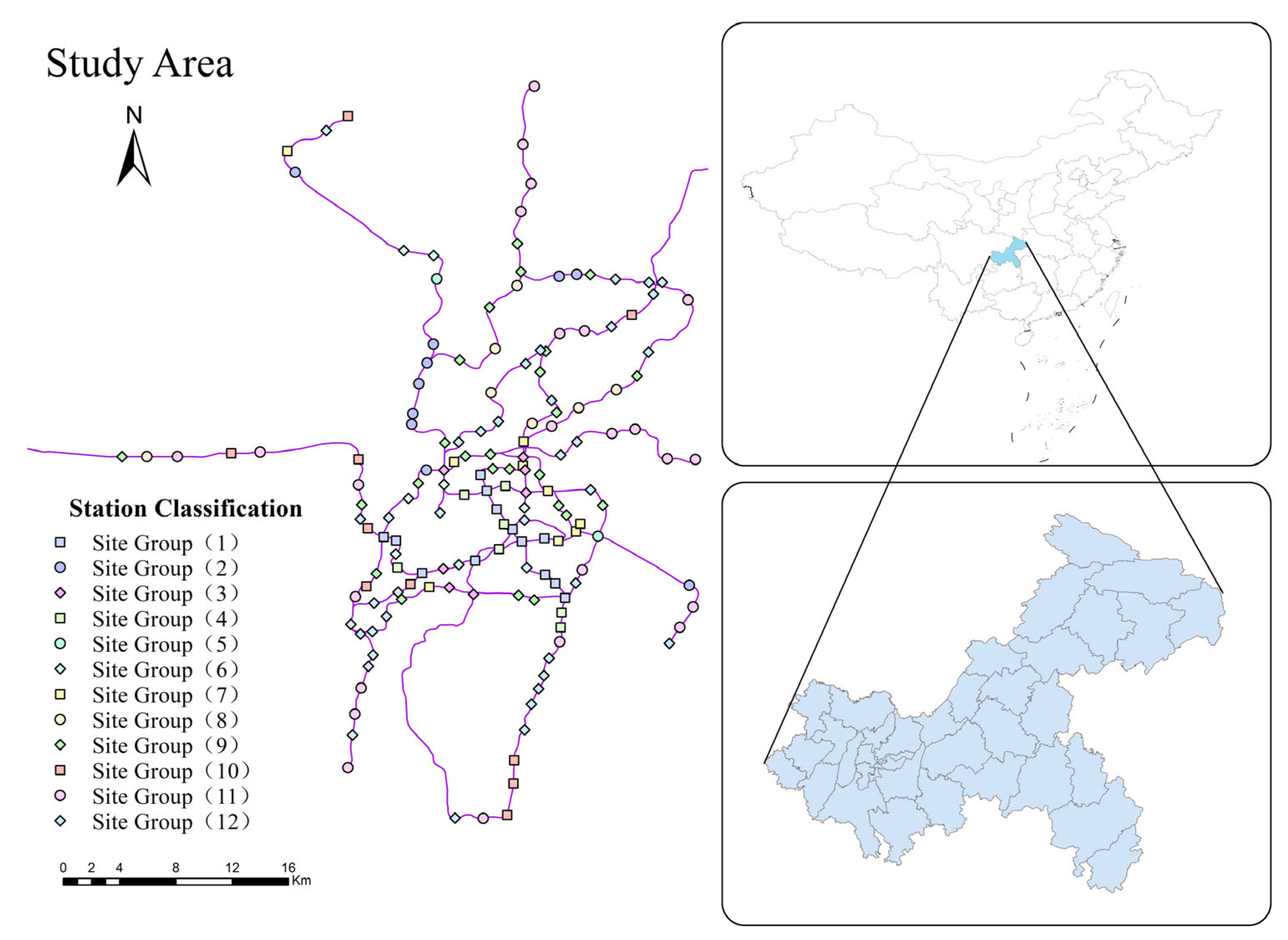
Through the two-stage clustering procedure, Chongqing’s urban rail transit stations were classified into 12 distinct types (Table 3). Their spatial distribution aligns closely with the city’s mountainous structure, reflecting the interplay between topography, land use, and the transit network. To better reveal these spatial characteristics and regional contrasts, the classification results were mapped in ArcGIS 10.7, as presented in Figure 6.

• Central Urban Clusters. These areas are dominated by high-value bus-transfer congested stations. Such stations are typically located in relatively flat and highly developed districts, where commercial, office, and public service facilities are densely concentrated. Passenger flows are complex, encompassing commuting, business, and local travel needs. A well-developed bus network and high transfer density mitigate the walking barriers imposed by hilly terrain, thereby extending metro accessibility. However, this also results in persistently high crowding during peak periods. This pattern demonstrates how dense development and integrated transport infrastructure in central areas can overcome terrain constraints, forming high-intensity, high-accessibility ridership hubs.
• Peri-Cluster Areas. These zones are primarily characterized by low-value pedestrian-transfer comfort-oriented stations. Typically located in transitional urban–rural belts, they feature lower development intensity and weaker public transit coverage. Passengers in these areas primarily rely on walking to complete the first- and last-mile. Although crowding is low and travel experience relatively comfortable, the overall transport efficiency and urban functionality remain limited, reflecting the weaker attractiveness of such areas.
• Steep Slope Areas. In areas where the road slope exceeds 15%, stations are mainly based on Low-value balanced-transfer comfort-oriented type. These stations are located in steep areas, near mountaintops or bridgeheads, where significant terrain changes and narrow winding roads hinder traditional bus operations, resulting in some passengers having to rely on walking. But Chongqing has introduced “alley buses” in some steep neighborhoods to strengthen bus connectivity. However, its limited scale, incomplete coverage, and capacity limitations make it unable to fully compensate for the transmission gap caused by terrain.

The classification framework developed here, by coupling built environment with flow characteristics, provides a theoretical foundation for understanding the spatial heterogeneity of ridership mechanisms in mountainous-city metro systems. It also establishes the basis for subsequent analyses of fare elasticity differences. Differentiating stations in this manner can inform more targeted time-of-day pricing and transfer optimization strategies, thereby enhancing the precision and efficiency of operations in mountainous urban rail systems.

4. Differences in Fare Elasticity Among Station Types

4.1. Data Sources

This study investigates how passenger travel behavior responds to fare adjustments under time-of-day pricing strategies. To first verify the stability of fare elasticity within the same station type and establish acceptable error bounds, two representative categories among the twelve classified station types were selected for initial analysis: high-value bus-transfer congested stations and high-value pedestrian-transfer congested stations. These two categories were chosen because they capture the most distinct characteristics in terms of transfer modes and congestion patterns, representing the upper bounds of passenger sensitivity to fare changes. Demonstrating stability within these extreme categories provides a justified basis for assuming that other station types with similar structural and operational characteristics would exhibit comparable intra-type fare elasticity. Once stability was confirmed, surveys were extended to additional station categories along Line 3 of the Chongqing Rail Transit system.

The survey adopted a combined online and offline approach, targeting passengers randomly at station platforms and rest areas to ensure a representative sample of metro users. The questionnaire consisted of two parts: the first part collected passengers’ socio-demographic information (gender, age, occupation, income) and trip characteristics (purpose, frequency, distance, fare, duration) [39,40], reflecting actual travel behavior (RP); the second part examined passengers’ acceptance of time-based fare pricing, capturing intended responses under hypothetical fare adjustments (SP). A pilot survey of 50 respondents was conducted to verify clarity and comprehension, and technical terms related to time-of-day pricing were simplified based on feedback.

As a result, a total of 557 questionnaires were distributed, of which 506 were valid, resulting in an effective response rate of 90.8%. These responses provide a reliable dataset for analyzing how fare variations influence passenger travel behavior and modal shifts across different station types.

4.2. Intra-Type Fare Elasticity Stability

During peak hours, passengers generally show low overall price elasticity for switching completely to alternative transport modes outside the rail system (e.g., buses, taxis, ride-hailing). This outcome stems from the highly purpose-driven and time-rigid nature of commuting trips [41]. To ensure punctuality for work or school, passengers place greater emphasis on time costs than on fare costs. Consequently, even when fares change, most passengers adhere to their original schedules rather than risk longer or less reliable alternative modes. This suggests that fare incentives alone are insufficient to divert passengers entirely away from rail during peak periods. Accordingly, this study focuses on encouraging temporal shifts between peak and off-peak periods within the rail system. A critical prerequisite is verifying that fare elasticity is consistent and stable within the same station type, ensuring that time-of-day pricing generates predictable differential effects across categories.

To quantitatively evaluate passengers’ sensitivity to fare adjustments, this study introduces fare elasticity coefficient (E), which measures the relative change in passenger transfer ratio resulting from a change in fare. A higher elasticity value indicates that passengers are more responsive to fare changes, whereas lower values suggest weaker sensitivity. The definition of the elasticity coefficient is shown in Equation (5).

$$E={\displaystyle \frac{\mathsf{\Delta }Q/Q}{\mathsf{\Delta }P/P}}={\displaystyle \frac{\mathsf{\Delta }Q}{\mathsf{\Delta }P}}\times {\displaystyle \frac{P}{Q}}$$

(5)

where ΔQ is the change in the passenger transfer ratio before and after fare adjustment; Q is the initial passenger transfer ratio; ΔP is the change in the ticket price; P is the initial fare level.

The parameter $P$ is assumed to be 1 for standardization, as the analysis focuses on relative fare changes rather than absolute values. Fare adjustments were simulated under several policy scenarios: peak-hour fare increases of 20%, 40%, and 60%, and off-peak fare reductions of 20%, 40%, and 60%. The average rate of fare change (40%) was used as the representative value for calculating elasticity. The elasticity coefficient thus reflects the degree to which passengers adjust their departure time within the metro system while also capturing, to a lesser extent, modal adjustments to alternative transport modes.

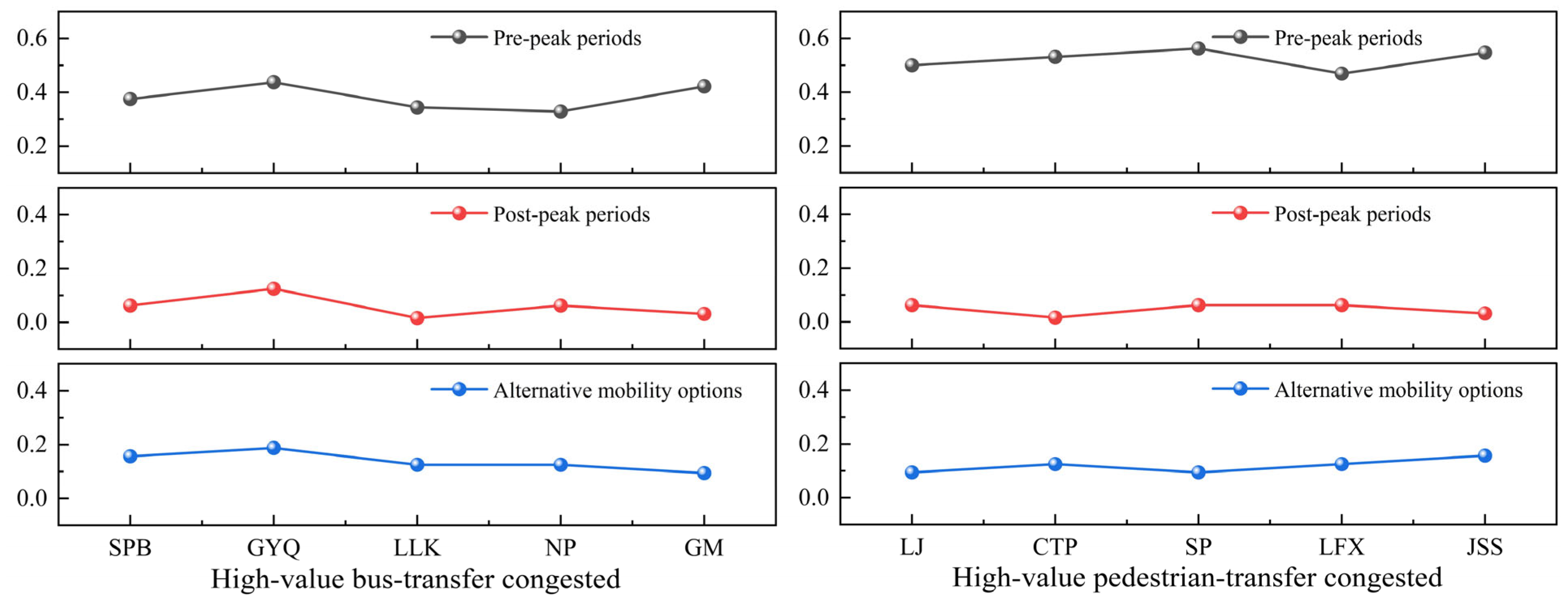
To examine intra-type variability, questionnaire responses from ten representative stations were analyzed, with results presented in Figure 7. The results show that morning-peak fare elasticity coefficients at high-value bus-transfer congested stations concentrate within [0.33, 0.44] (standard deviation ± 0.048), while those at high-value pedestrian-transfer congested stations fall within [0.47, 0.56] (standard deviation ± 0.038). These findings indicate that stations of the same type exhibit significantly clustered fare elasticity with controllable variability. This validates the reliability of the station classification model in capturing fare sensitivity and establishes a robust basis for subsequent analysis of cross-type differences in transfer elasticity across peak periods.

4.3. Inter-Type Differences in Fare Elasticity

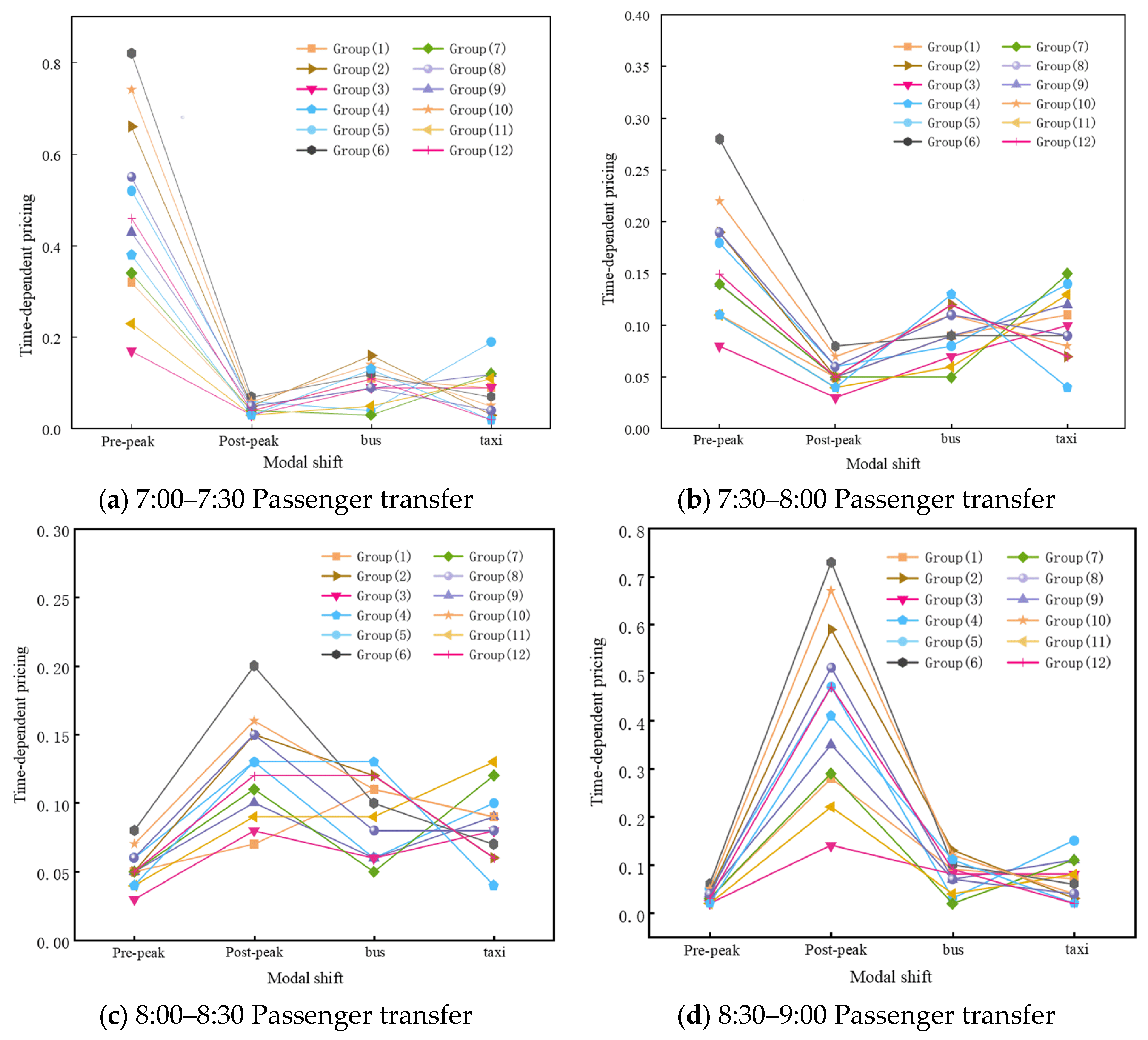
Passenger transfer elasticity across different time intervals was calculated using survey data from various station types, as illustrated in Figure 8. The results indicate clear heterogeneity among station categories. At low-value stations, transfer elasticity is consistently higher than at high-value stations, reflecting the relatively lower economic status of surrounding passengers and their greater fare sensitivity. Congested stations show higher elasticity than comfort-oriented stations; the more crowded the carriages, the lower the ride comfort, and thus fare changes exert a stronger influence. At bus-transfer stations, fare adjustments lead to greater shifts toward bus use, whereas at pedestrian-transfer stations, elasticity is more pronounced for shifting to pre-peak or post-peak periods. Balanced-transfer stations exhibit moderate elasticity. In terms of timing, passengers departing between 7:00–7:30 display higher elasticity for shifting to pre-peak, while those departing between 8:30–9:00 show greater elasticity for shifting to post-peak. By contrast, elasticity during 7:30–8:30 is relatively lower, as the time cost of shifting to either pre-peak or post-peak is greater.

To make the comparison of fare elasticity across station types and departure windows statistically explicit, we further summarized the station-level elasticity coefficients by station type and time slice. For each station type and departure window (7:00–7:30, 7:30–8:00, 8:00–8:30, and 8:30–9:00), the estimated coefficients for shifts to pre-peak and post-peak periods were taken as measures of temporal fare elasticity within the rail system. The twelve station types were treated as independent observational units. For each departure window, we calculated the mean elasticity across station types and its 95% confidence interval using a t distribution. Differences in elasticity between time slices were assessed using paired t-tests on station-type means with Holm adjustment to control the familywise error rate. The resulting station-type-specific estimates are reported in

Table 4. Pre-peak time-shift elasticity by station type and departure time slice.

Site Group	7:00–7:30	7:30–8:00	8:00–8:30	8:30–9:00
1	0.32	0.11	0.05	0.03
2	0.52	0.18	0.06	0.05
3	0.43	0.14	0.05	0.04
4	0.17	0.08	0.03	0.02
5	0.34	0.14	0.05	0.03
6	0.23	0.11	0.04	0.02
7	0.66	0.19	0.05	0.04
8	0.82	0.28	0.08	0.06
9	0.74	0.22	0.07	0.05
10	0.38	0.11	0.04	0.02
11	0.55	0.19	0.06	0.04
12	0.46	0.15	0.05	0.03
Mean across station types (95% CI)	0.47 (0.34–0.59)	0.16 (0.12–0.19)	0.05 (0.04–0.06)	0.04 (0.03–0.04)

.

In terms of departure timing, the estimates in Table 4 and the cross-type averages highlight strong time-of-day contrasts in pre-peak shifts. Mean pre-peak elasticity across station types is 0.47 for passengers departing between 7:00–7:30, but falls to 0.16 in 7:30–8:00, 0.05 in 8:00–8:30, and 0.04 in 8:30–9:00. Paired t-tests on station-type means show that all pairwise differences between these four windows are statistically significant after Holm adjustment (p < 0.001). This confirms that pre-peak shift elasticity is highest for departures at the very beginning of the peak period (7:00–7:30) and substantially lower during the core peak (7:30–8:30).

For post-peak shifts, the pattern reverses at the tail of the peak period. Mean post-peak elasticity across station types is 0.046 for departures in 7:00–7:30 and 0.053 in 7:30–8:00, increases to 0.12 for 8:00–8:30, and reaches 0.43 for departures in 8:30–9:00. Again, all pairwise contrasts between departure windows are statistically significant with Holm-adjusted (p < 0.001). Thus, passengers departing in 8:30–9:00 are much more responsive to fare incentives that encourage shifting to later, post-peak times, while those in the core peak (7:30–8:30) exhibit the lowest temporal elasticity. Together, these findings quantitatively corroborate the earlier qualitative statements that fare incentives are more effective at the edges of the peak period (7:00–7:30 and 8:30–9:00) and less effective in the core 7:30–8:30 window, where the time cost of shifting to either pre-peak or post-peak is highest.

The analysis primarily focuses on passengers’ temporal adjustment behaviors within the rail system rather than complete modal shifts. Time-of-day pricing mainly aims to encourage passengers to retime their departure to less crowded periods, thereby alleviating peak congestion. Most observed changes reflect shifts to pre-peak or post-peak intervals, particularly at pedestrian-transfer stations where flexible schedules allow earlier or later travel. In contrast, only a small fraction of passengers—mainly at bus-transfer stations—reported switching to bus services when fare differentials were large. Thus, fare variations primarily induce departure-time redistribution within the metro system, while modal shifts remain a limited, secondary response influenced by bus network availability. These findings establish a clear correspondence between station classification and fare elasticity differences, providing a theoretical basis for understanding heterogeneous travel demand in mountainous-city metro systems.

5. Station Type Sensitivity Analysis

This chapter investigates the determinants of fare elasticity and their implications for station classification. First, a multiple linear regression model is applied to identify key explanatory indicators of fare elasticity. Then, focusing on variables that can be shaped through urban planning, we employ a multinomial logistic regression to simulate how marginal changes alter the probability of station type, thereby conducting a sensitivity analysis.

5.1. Identification of Key Factors Affecting Fare Elasticity

To further examine the factors influencing passengers’ fare sensitivity across different station types, a multiple linear regression model was constructed. The dependent variable in this model is the fare elasticity coefficient (E). The independent variable refers to the factor selected for clustering stations, and its independent variables and their original parameter symbols are R_b (number of bus routes), S_b (number of bus stations), R_a (number of alley bus routes), D_n (average transfer distance), C_r (road growth coefficient), I (average longitudinal slope), P_a (number of parking lots), H_μ (average housing price), H_σ (standard deviation of housing price), C_up (average congestion during upstream peak hours), and C_down (average congestion during downstream peak hours). The general form of the regression model is shown in Equation (6) below.

$$\begin{gathered} E={\beta }_0+{\beta }_1·R_b+{\beta }_2·S_b+{\beta }_3·R_a+{\beta }_4·D_t+{\beta }_5·C_r+{\beta }_6·I+{\beta }_7·P_a+{\beta }_8 \\ ·H_{\mu }+{\beta }_9·H_{\sigma }+{\beta }_{10}·C_{up}+{\beta }_{11}·C_{down}+\epsilon \end{gathered}$$

(6)

The analysis of variance results, summarized in

Table 5. ANOVA Results for Multiple Linear Regression Model.

Source	Sum of Squares	df	Mean Square	F	Sig.
Regression	1.768	11	0.161	9.890	0.000
Residual	2.388	147	0.016
Total	4.156	158

, indicate that the model is statistically significant (F = 9.890, p < 0.01). Moreover, all explanatory variables exhibit variance inflation factors below 10, as reported in

Table 6. Significance Tests of Partial Regression Coefficients.

Variable	Unstandardized Coefficients		Standardized Coefficients	t	Sig.	VIF
	B	Std. Error	Beta
Constant	0.738	0.061	–	12.084	0.000	–
Upstream congestion level	0.155	0.036	0.345	4.240	0.000	1.691
Downstream congestion level	0.112	0.035	0.273	3.239	0.001	1.816
Number of parking facilities	−0.003	0.001	−0.292	−3.066	0.003	2.327
Average housing price	−2.808 × 10−5	0.000	−0.492	−6.569	0.000	1.438
Housing price variation	1.206 × 10−6	0.000	0.017	0.216	0.829	1.542
Average slope	1.829 × 10−5	0.001	0.002	0.030	0.976	1.105
Growth coefficient	−0.003	0.001	−0.180	−2.122	0.035	1.832
Number of bus stops	0.004	0.004	0.095	1.078	0.283	1.974
Number of bus routes	−0.004	0.001	−0.343	–3.573	0.000	2.357
Number of feeder buses	0.016	0.015	0.073	1.074	0.285	1.190
Average transfer distance	4.027 × 10−5	0.000	0.027	0.395	0.693	1.188

, suggesting that multicollinearity is not a major concern and that the coefficient estimates are robust. These findings confirm the validity of the regression framework, providing a reliable basis for subsequent examination of individual factors and their influence on fare elasticity across different station types.

The regression coefficient analysis identifies six key determinants of fare elasticity. Upstream and downstream peak congestion are positively correlated with elasticity, indicating that heavier passenger loads increase sensitivity to fare changes. In contrast, greater parking availability and higher average housing prices are negatively associated with elasticity, suggesting that passengers in more affluent or car-oriented areas are less responsive to fare adjustments. Similarly, the number of bus routes and the road network growth factor exert significant negative effects, reflecting that enhanced feeder-bus services and improved walkability mitigate sensitivity to fare changes. Other variables, including housing price variability, average slope, bus stop density, alley-bus services, and transfer distance, do not exhibit statistically significant effects. Overall, passenger crowding, parking supply, local housing prices, bus route provision, and road network growth emerge as the principal factors shaping fare elasticity, providing strong explanatory power and establishing a solid foundation for subsequent sensitivity analyses and policy recommendations.

To verify the reliability of the multiple linear regression, we conducted standard diagnostic tests. Shapiro–Wilk (W = 0.99, p = 0.33) and Jarque–Bera (χ² = 2.01, p = 0.37) indicate that residuals are approximately normal. Breusch Pagan (LM = 26.13, p = 0.006) and White (LM = 99.24, p = 0.045) tests reveal heteroskedasticity, so heteroskedasticity robust (HC3) standard errors were used when assessing significance. Under robust SEs, the six main determinants—upstream and downstream congestion levels, number of parking facilities, average housing price, road growth coefficient, and number of bus routes—remain statistically significant at the 5% level, while other variables are still non-significant. Cook’s distance identifies a small number of potentially influential stations, but refitting the model without them does not materially change the estimated coefficients or their significance. Given the spatial clustering of stations, Moran’s I on the residuals shows modest positive spatial autocorrelation, suggesting that some unobserved spatially varying factors remain and should be addressed in future work using more advanced spatial or instrumental-variable models when suitable data become available.

5.2. Sensitivity of Station Classification to Key Factors

The regression analysis indicates that the number of bus routes and the growth coefficient significantly affect fare elasticity. Unlike socioeconomic variables such as housing prices, these two factors can be directly influenced through urban planning and transportation management, thereby indirectly reflecting fare changes. To further examine whether their variations affect station classification, a multinomial logistic regression model was applied, since the dependent variable (station type) is unordered categorical. By systematically adjusting the values of bus routes and growth coefficient within their observed ranges while holding other variables constant, the marginal effects on classification probabilities were simulated. Log-Likelihood of the fitted model is −254.02, Likelihood Ratio Test yields χ² = 244.59 with 22 degrees of freedom (p < 0.001), and McFadden pseudo R² is 0.325. These values indicate that the MNL model provides a statistically significant and substantively meaningful fit to the observed station classifications. These simulations should be interpreted as indicative policy pathways rather than causal effects, and are intended to complement the regression-based explanations of fare sensitivity.

Sensitivity analysis entails altering the target variable under controlled conditions and observing changes in the most probable station type and its classification probability. A benchmark station must satisfy both high sensitivity (classification uncertainty) and high representativeness (features close to sample mean). Based on these criteria, Huayansi Station was selected as the benchmark: its maximum classification probability was only 0.54, reflecting high uncertainty, while its key features were closest to the overall mean, making it an ideal candidate for marginal effect simulation.

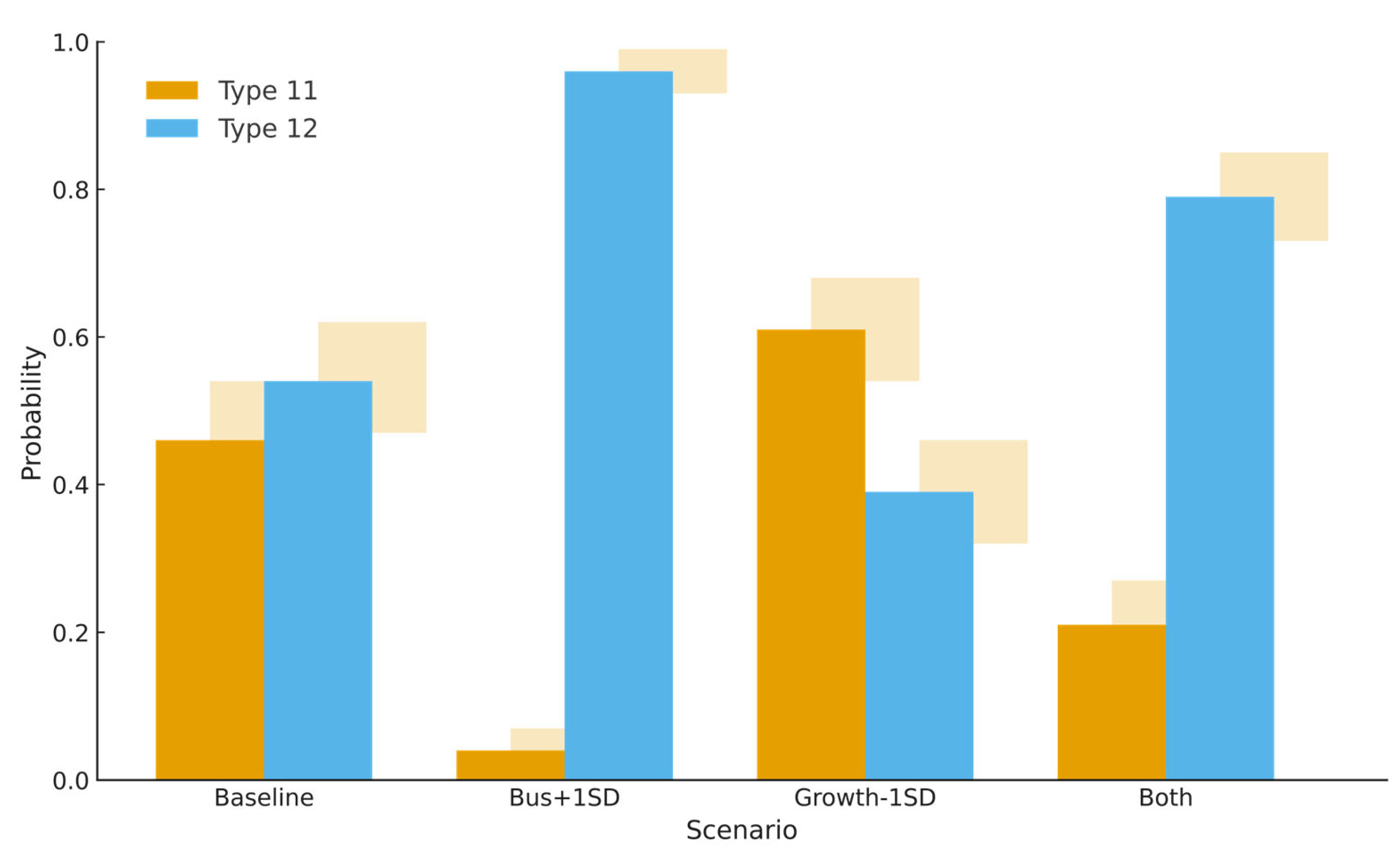
Based on Huayansi Station, three scenarios were simulated: (1) a one-standard-deviation (SD) increase in the number of bus routes, (2) a one-SD decrease in the growth coefficient, and (3) simultaneous changes in both. The trained multinomial logistic regression model was then used to compute classification probabilities across all categories, as shown in Figure 9 which illustrates how changing the two key features of the baseline station affects its classification probability. These bars quantify the probability of each type. For example, under Scenario 2, the station shifts toward Type 11 (low-value pedestrian-access comfort type), with a Type 11 probability of 0.61 (SE = 0.04; 95% CI: 0.53–0.69) and a reduced Type 12 probability of 0.39 (SE = 0.04; 95% CI: 0.31–0.47). The corresponding change in the Type 12 probability (−0.15; SE = 0.06; 95% CI: −0.26 to −0.04) indicates that enhanced pedestrian accessibility tends to transform balanced-access stations toward pedestrian-access types.

The results indicate that increasing the number of bus routes by one SD did not alter the fundamental station type but sharply raised the probability of classification as Type 12 (low-value balanced-access comfort type) from 0.54 (SE = 0.04; 95% CI: 0.46–0.62) to 0.96 (SE = 0.02; 95% CI: 0.93–0.99). This suggests that enhancing bus supply for balanced-access stations primarily reinforces their existing classification while suppressing transitions to other types. By contrast, improving the growth coefficient (lower values) induced a type shift: the station transitioned from Type 12 to Type 11 (low-value pedestrian-access comfort type), with a transition probability of 0.61 (SE = 0.04; 95% CI: 0.53–0.69). This indicates that better pedestrian accessibility may shift a station’s classification from “balanced-access” to “pedestrian-access.” However, Type 12 still retained a 0.39 (SE = 0.04; 95% CI: 0.31–0.47) probability, reflecting partial persistence of the original type.

When both factors changed simultaneously, the station classification reverted to Type 12, but with a lower probability (0.79 (SE = 0.03; 95% CI: 0.73–0.85)) than in the single-variable bus route scenario, while Type 11 emerged as the secondary outcome with a probability of 0.21 (SE = 0.03; 95% CI: 0.15–0.27). This suggests that the influence of bus routes is stronger, but the effect of the growth coefficient remains, manifesting as a redistribution of probabilities rather than elimination. The two factors thus interact in a non-additive manner, with competing influences on station classification.

In summary, the combined use of multiple linear regression and multinomial logistic regression identifies congestion level, parking facilities, housing prices, bus routes, and growth coefficient as key determinants of fare elasticity. Among these, bus routes tend to stabilize existing station classifications, whereas the growth coefficient may induce functional transformation. These findings shed light on the origins of heterogeneous passenger demand in mountainous urban rail transit systems and provide a theoretical basis and planning guidance for designing differentiated time-based pricing strategies tailored to station types.

6. Discussion

This study contributes to the growing body of literature on fare elasticity and spatial heterogeneity in urban rail systems by revealing how station-level characteristics influence passengers’ behavioral responses under time-differentiated pricing. The results reaffirm the working hypothesis that fare sensitivity is not uniform across the network but shaped by a combination of spatial, socioeconomic, and operational factors. From a comparative perspective, the results are broadly consistent with previous studies conducted in other large cities, which have shown that passengers at peripheral or lower-income stations tend to be more price-responsive, whereas those at central, high-income stations exhibit lower elasticity. However, this study extends existing evidence by demonstrating that such patterns are amplified in mountainous contexts, where steep topography and limited multimodal connectivity constrain travel flexibility. The strong differentiation observed among the twelve identified station types confirms that topography and transfer conditions are critical determinants of fare responsiveness in complex urban environments.

In addition, the interplay between bus connectivity and pedestrian accessibility highlights the importance of transfer design in shaping behavioral outcomes. Similar to findings from studies in Zurich and Hong Kong, higher bus-route density enhances passengers’ modal substitution options, thereby increasing overall elasticity. Conversely, stations located in steep or poorly connected areas show reduced flexibility, not because of low fare awareness, but due to physical and transfer-related barriers. This suggests that infrastructure improvements can complement pricing strategies to achieve more balanced demand distribution. The results also provide policy insights for urban rail systems with comparable geographical or structural challenges. Time-of-day pricing can be most effective when targeted toward specific station types rather than applied uniformly. By aligning fare incentives with local transfer conditions and socioeconomic characteristics, operators can achieve higher efficiency and fairness in demand management. Such differentiation supports the sustainability goals of urban transport systems by reducing peak-period congestion, improving energy utilization, and encouraging equitable access to transit services.

Future research should aim to validate these findings using revealed-preference data derived from smart-card transactions following actual fare adjustments. Comparative analyses across multiple mountainous and non-mountainous cities would further clarify how urban form moderates fare elasticity. Finally, integrating behavioral simulation or dynamic assignment models could help forecast long-term impacts of differentiated pricing on network performance and equity outcomes.

7. Conclusions

Taking Chongqing’s metro system—characterized by distinct mountainous terrain—as the research context, this study integrates multidimensional indicators, including topography, transfer accessibility, surrounding economic conditions, and in-train congestion, to develop a station classification framework and a fare sensitivity analysis model for mountainous cities. The key findings are as follows:

(1) Mountain-Specific Station Classification: Based on 11 indicators such as road slope, bus feeder density, average housing price, and peak-hour congestion, metro stations were clustered into 12 categories. These station types display clear functional and ridership heterogeneity. For example, central cluster stations are typically high-value, bus-connected, and highly congested, while peripheral cluster stations are often low-value, pedestrian-dependent, and relatively comfort-oriented. Stations located in steep-slope areas commonly experience poor transfer conditions and severe peak-hour congestion.

(2) Heterogeneity of Fare Elasticity: Fare elasticity differs significantly across station categories, showing clear stratification. Low-value pedestrian-transfer congested stations exhibit the highest elasticity, with pre-peak transfer elasticity reaching up to 0.82, indicating pronounced fare sensitivity. In contrast, high-value bus-transfer comfort-oriented stations display the lowest elasticity, as low as 0.17, with passengers more inclined to maintain fixed schedules. Moreover, the analysis reveals that lower economic levels and higher in-train crowding are strongly associated with greater fare responsiveness. Passengers at bus-transfer stations are more likely to shift toward conventional bus services under fare adjustments, while those at pedestrian-transfer stations tend to adjust their departure times.

(3) Key Determinants and Planning Implications: Fare elasticity is primarily influenced by sectional passenger crowding, surrounding housing price levels, and bus connectivity. Among these, the number of bus routes and the road network growth factor represent core variables that can be modified through planning interventions. Sensitivity analysis shows that expanding bus routes can substantially alter station type probabilities, increasing the likelihood of bus-transfer classifications, while reducing the road growth factor (enhancing walkability) can induce transitions toward pedestrian-transfer types. When adjusted simultaneously, these two factors exhibit interactive and competing effects, underscoring that station functionality is shaped by the coupling of multiple influences.

Based on these insights, differentiated strategies for time-of-day pricing can be designed. Larger pre-peak discounts should be considered for low-value congested stations to maximize diversion effects; flexible, dynamic fares can be applied at high-value comfort-oriented stations to encourage time-shifting of potential passengers; and priority should be given to improving bus coverage and pedestrian accessibility to indirectly influence station attributes and fare sensitivity. Overall, this research contributes to sustainability by providing a quantitative, station-type-based framework for measuring and monitoring how time-of-day pricing affects passenger behavior in mountainous urban rail systems. The identified relationships between fare elasticity, congestion, accessibility, and built environment conditions offer actionable evidence for designing equitable and environmentally friendly pricing and service strategies that reduce peak-hour overcrowding, improve the use of low-carbon rail capacity, and support more sustainable urban development in mountainous cities.

References

- Tokyo Metro. Business Situation; Tokyo Metro: Tokyo, Japan, 2024; Available online: https://www.tokyometro.jp/corporate/enterprise/passenger_rail/transportation/lines/index.html (accessed on 26 October 2025).
- Tokyo Metro. Traffic Performance by Station; Tokyo Metro: Tokyo, Japan, 2024; Available online: https://www.tokyometro.jp/lang_en/corporate/enterprise/transportation/ranking/index.html (accessed on 26 October 2025).
- Metropolitan Transportation Authority (MTA). Subway and Bus Ridership for 2024; MTA: New York City, NY, USA, 2024; Available online: https://www.mta.info/agency/new-york-city-transit/subway-bus-ridership-2024 (accessed on 26 October 2025).
- Paris Régie des Transports Parisiens (RATP). Trafic Annuel Entrant par Station du Réseau Ferré 2021; RATP: Paris, France, 2021; Available online: https://data.ratp.fr/explore/dataset/trafic-annuel-entrant-par-station-du-reseau-ferre-2021/table/?sort=-rang (accessed on 26 October 2025).
- Yang, H.; Tang, Y. Managing rail transit peak-hour congestion with a fare-reward scheme. Transp. Res. Part B Methodol. 2018, 110, 122–136. [Google Scholar] [CrossRef]
- Gaymer, S. Early Bird Initiative–Evaluation Assessment; Department of Transport: Melbourne, VIC, Australia, 2008. [Google Scholar]
- Halvorsen, A.; Koutsopoulos, H.; Ma, Z.; Zhao, J. Demand management of congested public transport systems: A conceptual framework and application using smart card data. Transportation 2020, 47, 2337–2365. [Google Scholar] [CrossRef]
- Adnan, M.; Nahmias Biran, B.-h.; Baburajan, V.; Basak, K.; Ben-Akiva, M. Examining impacts of time-based pricing strategies in public transportation: A study of Singapore. Transp. Res. Part A Policy Pract. 2020, 140, 127–141. [Google Scholar] [CrossRef]
- Zhang, X. Study on the Time Differential Pricing Model of Urban Rail Transit. Master’s Thesis, Beijing Jiaotong University, Beijing, China, 2016. [Google Scholar]
- 16 Stations Will Implement Low-Peak Fares from December 28. Available online: https://www.beijing.gov.cn/gongkai/hygq/201512/t20151228_1837361.html (accessed on 26 October 2025).
- The Number of Low-Peak Preferential Fare Stations Has Increased to 24, from 70% to 50%. Available online: https://jtw.beijing.gov.cn/xxgk/xwfbh/201912/t20191209_1007459.html (accessed on 26 October 2025).
- Start Your Day Earlier & Enjoy a Fare Discount! Available online: https://www.mtr.com.hk/archive/ch/pdf/mtr-early-bird-leaflet.pdf (accessed on 26 October 2025).
- Yao, X.; Chen, L.; Zhao, P.; Zou, Q.; Wang, Z. Exploring travelers’ responses to a prepeak discount fare policy and optimizing the pricing strategy to ease peak congestion: The case of Beijing subway. Transp. Res. Part A Policy Pract. 2025, 191, 104335. [Google Scholar] [CrossRef]
- Korf, J.; Demetsky, M. Analysis of rapid transit access mode choice. Transp. Res. Rec. 1981, 817, 29–35. [Google Scholar]
- Bertolini, L. Spatial Development Patterns and Public Transport: The Application of an Analytical Model in The Netherlands. Plan. Pract. Res. 1999, 14, 199–210. [Google Scholar] [CrossRef]
- Zemp, S.; Reusser, D.; Scholz, R. Classifying railway stations for strategic transport and land use planning. J. Transp. Geogr. 2011, 19, 670–679. [Google Scholar] [CrossRef]
- Schimek, P. Dynamic Estimates of Fare Elasticity for U.S. Public Transit. Transp. Res. Rec. J. Transp. Res. Board 2015, 2538, 96–101. [Google Scholar] [CrossRef]
- Pang, L.; Ren, L.; Zhang, Z.; Yun, Y. Metro Station Classification Based on Boarding and Alighting Passenger Flows and Ridership Impact Factors. J. Transp. Syst. Eng. Inf. Technol. 2023, 23, 184–193. [Google Scholar]
- Wang, L.; Shi, L.; Wang, Y.; Zhang, G.; Du, Y. Classification Method of Urban Rail Stations Under the Concept of Mobility as Service. J. Wuhan Univ. Technol. (Transp. Sci. Eng.) 2025, 49, 232–236. [Google Scholar]
- Wang, Y.; Wang, Z.; Zhao, F. Integrating Node-Place Model with Shapley Additive Explanation for Metro Ridership Regression. IEEE Trans. Intell. Transp. Syst. 2025, 1–10. [Google Scholar] [CrossRef]
- Xing, X.; Wan, L.; Luo, F. Demand prediction for shared bicycles around metro stations incorporating STAGCN. PLoS ONE 2025, 20, e0328452. [Google Scholar] [CrossRef] [PubMed]
- Wallimann, H.; Blättler, K.; Arx, W. Do price reductions attract customers in urban public transport? A synthetic control approach. Transp. Res. Part A Policy Pract. 2023, 173, 103700. [Google Scholar] [CrossRef]
- Rahman, A. A GIS-based, microscale walkability assessment integrating the local topography. J. Transp. Geogr. 2022, 103, 103405. [Google Scholar] [CrossRef]
- Gao, L.; Chong, H.; Zhang, W.; Li, Z. Nonlinear effects of public transport accessibility on urban development: A case study of mountainous city. Cities 2023, 138, 104340. [Google Scholar] [CrossRef]
- Holmgren, J. Meta-Analysis of Public Transport Demand. Transp. Res. Part A Policy Pract. 2007, 41, 1021–1035. [Google Scholar] [CrossRef]
- Kholodov, Y.; Jenelius, E.; Cats, O. Public Transport Fare Elasticities from Smartcard Data: Evidence from a Natural Experiment. Transp. Policy 2021, 105, 35–43. [Google Scholar] [CrossRef]
- Metropolitan Transportation Authority (MTA). Subway Origin–Destination Ridership Dataset and Annual Report; MTA: New York City, NY, USA, 2023; Available online: https://www.mta.info/article/introducing-subway-origin-destination-ridership-dataset (accessed on 26 October 2025).
- Transport for London (TfL). Annualised Station Entry and Exit Counts (Open Data); TfL: London, UK, 2023. Available online: https://tfl.gov.uk/info-for/open-data-users/our-open-data (accessed on 26 October 2025).
- Liu, Y.; Chen, B.; Zheng, Y.; Cheng, L.; Li, G.; Lin, L. ODMixer: Fine-Grained Spatial-Temporal MLP for Metro Origin-Destination Prediction. IEEE Trans. Knowl. Data Eng. 2025, 37, 5508–5522. [Google Scholar] [CrossRef]
- Wang, Y.; Zhang, Y.; Zhang, Y.; Ma, J. Dynamic real-time high-capacity ride-sharing model with subsequent information. IET Intell. Transp. Syst. 2020, 14, 742–752. [Google Scholar] [CrossRef]
- Sun, B.; Xu, Z.; Wei, M.; Wang, X. A study on the strategic behavior of players participating in air-rail intermodal transportation based on evolutionary games. J. Air Transp. Manag. 2025, 126, 102793. [Google Scholar] [CrossRef]
- MetroDB.org. Chongqing Metro Information Overview: Chongqing Urban Rail Passenger Flow Database. Available online: https://metrodb.org/index/chongqing.html (accessed on 26 October 2025).
- Peng, B.; Zhang, Y.; Wang, T.; Li, C. Exploring Nonlinear Effects of the Built Environment on Employment Behavior Among Older Adults: Evidence from Metro Station Catchment Areas. ISPRS Int. J. Geo-Inf. 2024, 13, 420. [Google Scholar] [CrossRef]
- Taylor, M.; Somenahalli, S. Distributions of walking access to public transport in Melbourne, Australia—Evidence on acceptable and tolerable walking distances. Int. J. Sustain. Transp. 2024, 18, 576–588. [Google Scholar] [CrossRef]
- Jiang, H.; Liu, R.; Luo, S. Understanding metro station areas’ functional characteristics via embedding representation: A case study of Shanghai. Sci. Rep. 2025, 15, 2725. [Google Scholar] [CrossRef]
- Zhou, Y.; Xia, H.; Yue, X.; Wang, P. Local outlier detection method based on improved K-means. Eng. Sci. Technol. 2024, 56, 66–77. [Google Scholar] [CrossRef]
- Wang, Q.; Hu, D. Optimization of K-Means Fast Clustering Algorithm Based on Spark. Comput. Simul. 2022, 39, 344–349. [Google Scholar] [CrossRef]
- Zhang, L.; Pei, T.; Meng, B.; Lian, Y.; Jin, Z. Two-Phase Multivariate Time Series Clustering to Classify Urban Rail Transit Stations. IEEE Access 2020, 8, 167998–168007. [Google Scholar] [CrossRef]
- Ma, S.; Weng, J.; Li, Z.; Sun, Y.; Lin, P. Influence Model of Metro Fare Preferential Policies on Passenger’s Off-peak Travel Behavior. J. Wuhan Univ. Technol. (Transp. Sci. Eng.) 2021, 45, 413–418. [Google Scholar] [CrossRef]
- Liu, Y.; Feng, X.; Jia, W.; Li, S.; Sha, X. Satisfaction in Urban Rail Transit Based on Characteristics of Passenger Groups. Transp. Res. 2020, 6, 95–101. [Google Scholar]
- Ding, X.; Hong, C.; Wu, J.; Zhao, L.; Shi, G.; Liu, Z.; Hong, H.; Zhao, Z. Research on Time-Based Fare Discount Strategy for Urban Rail Transit Peak Congestion. Urban Rail Transit 2023, 9, 352–367. [Google Scholar] [CrossRef]