Actuator Line Wall-Modeled Immersed Boundary Method for Predicting the Aerodynamic Performance of Wind Turbines

Abstract

This study addresses the trade-off between accuracy and efficiency in predicting the aerodynamics and wakes of large wind turbines. We developed a unified immersed boundary–actuator line framework with large-eddy simulation. The actuator line efficiently represents blade loading, while the immersed boundary method (IBM) with a wall model resolves near-blade turbulence. The solver uses a staggered Cartesian discretization and is accelerated by a hybrid CPU/GPU implementation. An implicit signed-distance geometry treatment and a ghost cell wall function based on Spalding’s law reduce near-wall grid requirements and eliminate body-fitted meshing. Flow past a three-dimensional cylinder at Re = 3900 validates the accuracy and good grid convergence of the IBM. For the wind turbine, three meshes show converged thrust and torque, with differences below 1% between the two finer grids. At the rated condition (U_∞ = 11.4 m/s), thrust and torque agree with STAR-CCM+ and FAST, with deviations of 6.3% and 1.2%, respectively. Parametric cases at 4–10 m/s show thrust and torque increasing nonlinearly with inflow, approximately quadratically, in close agreement with reference models. As wind speed rises, the helical pitch tightens, the wake broadens, and breakdown occurs earlier, consistent with stronger shed vorticity. The framework delivers high fidelity and scalability without body-fitted meshes, offering a practical tool for turbine design studies and extensible wind plant simulations.

1. Introduction

During this critical phase of global energy transition towards decarbonization, wind energy stands as one of the most technologically mature and widely commercialized renewable sources. Its development and utilization are expanding at an unprecedented rate [1,2]. However, as wind turbines continue to grow in unit capacity, conventional aerodynamic performance prediction methods based on empirical formulas or simplified models are proving inadequate to meet accuracy requirements in such complex flow environments. The accurate prediction of nonlinear phenomena, such as flow separation over blade surfaces, wake interference, and aeroelastic coupling, has become a fundamental bottleneck restricting the optimization of wind turbine design and the improvement of efficiency in wind farm clusters [3,4,5].

Numerical simulation methods for wind turbine aerodynamic performance have evolved from Blade Element Momentum (BEM) theory [6] to Computational Fluid Dynamics (CFDs) [7]. While BEM offers high computational efficiency, it exhibits significant inaccuracies in capturing three-dimensional rotational effects and unsteady flows. Fully resolved computational fluid dynamics (CFDs) approaches, such as large-eddy simulation (LES) or direct numerical simulation (DNS), can deliver high-fidelity results by explicitly resolving wind turbine geometries [8,9,10]. However, challenges such as time-consuming mesh generation and high computational cost limit practical application in engineering design and wind-farm-scale simulations [11,12] due to complex blade geometry and intricate moving boundary treatment. To balance accuracy and efficiency, actuator methods have been developed, among which the actuator line method (ALM) has emerged as a leading paradigm for simulating wind turbine wake physics and multi-turbine interactions [13,14]. The actuator line method [15,16] simplifies wind turbine blades into lines along which momentum sources are applied, simulating the aerodynamic effect of the blades on the flow by distributing body forces within the computational domain. A key strength of this method lies in its balance between computational efficiency and accuracy. Compared to fully geometry-resolving models that require high grid resolution, the ALM can employ relatively coarse meshes, substantially reducing computational expense. Furthermore, the ALM offers the flexibility to be coupled with various turbulence modeling approaches, such as Reynolds-Averaged Navier–Stokes (RANS), large-eddy simulation (LES), and hybrid RANS-LES methods, to accommodate different accuracy requirements [17,18,19].

The actuator line method (ALM) has been widely employed for predicting the aerodynamic performance of wind turbines across various scenarios. For fixed-bottom turbines, the ALM enables accurate prediction of power output, thrust load, and spanwise load distribution [20]. For instance, Antonio Cioffi et al. coupled a Gaussian Wake Model (GWM) with an actuator line model within OpenFAST to simulate the interactions between upstream and downstream turbines in a wind farm [21]. Behnam Moghadassian and Anupam Sharma developed an inverse design methodology based on the Actuator Disk Model (ADM) for the aerodynamic optimization of horizontal-axis wind turbine blades [22]. For floating offshore wind turbines, the ALM can be coupled with platform motion models to analyze the influence of platform motions on turbine aerodynamic performance and wake characteristics [23,24]. Alireza Arabgolarcheh et al. investigated these effects by applying an actuator line model to turbines mounted on four different platform types [24]. Their findings indicate that variations in relative velocity induced by platform motion led to wake deformation and time-dependent induced velocities. Furthermore, the ALM proves suitable for evaluating turbine performance under complex flow conditions, such as yawed operation, stall conditions, and flows within the turbulent atmospheric boundary layer [18,25]. Xue et al. utilized a Lattice Boltzmann Method coupled with large-eddy simulation (LBM-LES) to study the wake characteristics of the NREL 5 MW offshore wind turbine under yawed conditions [25]. They defined two dynamic yaw states to analyze the impact of different yaw rates. Similarly, Yin et al. [26] employed the LBM-LES method to predict the energy harvesting performance and wake evolution of a tidal stream turbine.

Enhancing model fidelity represents another critical direction for ALM development. The method exhibits limited capability in resolving near-field flow features, making it difficult to accurately capture three-dimensional effects near the blade root and tip, flow separation and reattachment, tip vortex shedding, and boundary layer transition. These limitations can lead to inaccuracies in predicting local blade loads and dynamic stall behavior. On the other hand, the Immersed Boundary Method (IBM) [27,28,29] has demonstrated unique potential in simulating rotating machinery flows by eliminating the need for grid regeneration around moving boundaries, though its accuracy in resolving near-wall flow structures requires further improvement. For example, Ouro [30] developed an immersed boundary (IB) method based on large-eddy simulation (LES) to achieve high-fidelity blade-resolved simulations of vertical-axis turbines. This approach couples a Lagrangian description of the turbine with a Eulerian treatment of the fluid dynamics, thereby avoiding the computationally expensive procedures associated with body-conforming grid methods, such as variable redistribution and/or interpolation at each time step. Liu and Hu [31] proposed an efficient numerical framework combining the actuator line (AL) method with an immersed boundary (IB) technique to predict wake interactions among multiple turbines. The rotor was represented using the AL model rather than a geometrically resolved approach. Wake dynamics behind several turbines in turbulent inflow were predicted via LES, while an efficient IB method incorporating moving least-squares (MLS) reconstruction was developed to simulate the nacelles and support structures of tidal turbines.

No single numerical method achieves an optimal balance between computational efficiency and simulation accuracy. Therefore, developing a hybrid computational approach capable of both accurately resolving near-wall flow features and efficiently simulating full-turbine and wind farm-scale flow fields has emerged as a critical scientific challenge for advancing wind turbine aerodynamic design theory and engineering applications. To establish a coupled framework that delivers both high fidelity and computational efficiency, we implemented a unified IBM-ALM framework with LES. The ALM efficiently represents the aerodynamic effect of the blades, while the IBM with LES resolves the turbulent flows near the blades. This work is distinct from the IBM-ALM method by Liu and Hu [31], in which the IBM is adopted to handle the tower, and the ALM is employed to consider the rotating blade. In contrast, the IBM and the ALM are coupled to consider the existence of the rotating blade. The force-flow interaction is treated in a unified manner at the filter scale, significantly enhancing the predictability of the near wake and local loads. In addition, the computational cost of the ALM remains a limiting factor when applied to wind farm-scale simulations or extensive parametric studies [21,32]. Therefore, a CPU/GPU (Central Processing Unit/Graphics Processing Unit) parallel framework was implemented to remarkably accelerate the computational speed of the present solver. We simulated the flows around a three-dimensional cylinder at Re = 3900 and the flows around the wind turbine to validate the accuracy of the present numerical model. Further, the aerodynamic characteristics and wake pattern of a wind turbine under different operating states were examined.

2. Numerical Method

2.1. N-S Equations and Their Numerical Implementation

At high Reynolds numbers, it is necessary to resolve the smallest dissipative eddies (Kolmogorov scale), requiring a large amount of grid points and resulting in extremely high computational costs. To relieve the requirement for grid resolution, the turbulence model of large-eddy simulation (LES) is introduced in this study. Compared to RANS, LES [33,34] directly resolves large-scale turbulent structures, while the smaller scales are modeled, enabling a good prediction of key unsteady dynamic processes such as flow separation, reattachment, and vortex shedding. The governing equations for LES can be derived by applying a filtering operation to Equations (1) and (2):

$${\displaystyle \frac{\mathsf{\partial }{\overline{u}}_i}{\mathsf{\partial }{x}_i}}=0$$

(1)

$${\displaystyle \frac{\mathsf{\partial }{\overline{u}}_i}{\mathsf{\partial }t}}+{\displaystyle \frac{\mathsf{\partial }({\overline{u}}_i{\overline{u}}_j)}{\mathsf{\partial }{x}_{ j}}}=-{\displaystyle \frac{1}{\rho }}{\displaystyle \frac{\mathsf{\partial }\overline{p}}{\mathsf{\partial }{x}_i}}+{\displaystyle \frac{\mathsf{\partial }}{\mathsf{\partial }{x}_{ j}}}\left(\upsilon {\displaystyle \frac{\mathsf{\partial }{\overline{u}}_i}{\mathsf{\partial }{x}_{ j}}}\right)-{\displaystyle \frac{\mathsf{\partial }{\overline{\tau }}_{ij}}{\mathsf{\partial }{x}_{ j}}}$$

(2)

where t is the time, subscript $\rho$ is the density, $\upsilon$ is the kinematic viscosity coefficient, i, j = 1, 2, and 3 denote components along the x-, y-, and z-directions in the Cartesian grid, $x_i$ and $x_j$ represent coordinate components in the Cartesian grid, $u_i$ and $u_j$ denote velocity components in the corresponding directions, the superscript $\overline{\phantom{,}}$ represents the variable applied filtering operation, ${\tau }_{ij}$ is the subgrid-scale stress tensor, and the overbar signifies filtered variables.

The generated ${\tau }_{ij}$ requires a modeling approximation to achieve the closure of Equations (1) and (2). Here, we employ a linear eddy viscosity model for the subgrid-scale stresses:

$${\tau }_{ij}-{\displaystyle \frac{1}{3}}{\delta }_{ij}{\tau }_{kk}={\upsilon }_t\left({\displaystyle \frac{\mathsf{\partial }{\overline{u}}_i}{\mathsf{\partial }{x}_{ j}}}+{\displaystyle \frac{\mathsf{\partial }{\overline{u}}_{ j}}{\mathsf{\partial }{x}_i}}\right)$$

(3)

where ${\delta }_{ij}$ is the Kronecker delta function, and ${\upsilon }_t$ is the eddy viscosity coefficient.

The eddy viscosity coefficient ${\upsilon }_t$ is an unknown quantity that requires modeling approximation. The WALE (Wall-Adapting Local Eddy-viscosity) model [35,36] is adopted because it naturally recovers the correct asymptotic behavior of the eddy viscosity near the wall without requiring explicit damping. Additionally, its formulation is relatively simple to solve. In contrast, the standard Smagorinsky model produces non-zero eddy viscosity at solid boundaries, necessitating ad hoc damping functions. In an IBM framework, where the grid is not body-fitted, applying these damping functions is geometrically complex and prone to error. The WALE model is expressed as follows:

$${\upsilon }_t={(C_w\Delta )}^2{\displaystyle \frac{{\left(S_{ij}^d{S}_{ij}^d\right)}^{3/2}}{{\left({\tilde{S}}_{ij}{\tilde{S}}_{ij}\right)}^{5/2}+{\left(S_{ij}^d{S}_{ij}^d\right)}^{5/4}}}$$

(4)

Here, $\Delta$ is the filtering scale, which is set as the local grid size. The $C_w$ is constant, which ranges within $0.55\le C_w\le 0.60$. The tensor $S_{ij}^d$ is defined as

$$S_{ij}^d={\displaystyle \frac{1}{2}}\left({\overline{g}}_{ij}^2+{\overline{g}}_{ji}^2\right)-{\displaystyle \frac{1}{3}}{\delta }_{ij}{\overline{g}}_{kk}^2$$

(5)

$${\overline{g}}_{ij}^2={\overline{g}}_{ik}{\overline{g}}_{kj}\mathrm{and} {\overline{g}}_{ ij}={\displaystyle \frac{\mathsf{\partial }{\overline{u}}_i}{\mathsf{\partial }{x}_{ j}}}$$

(6)

The present fluid solver employs a staggered Cartesian grid arrangement to solve the incompressible Navier–Stokes equations by an explicit finite-difference discretization, which facilitates GPU acceleration. The decoupling of the pressure and velocity in the momentum equations is achieved through a fractional-step approach. The temporal integration utilizes a second-order Runge–Kutta scheme (RK3) with total variation diminishing (TVD) properties, where both convective and diffusive terms are treated explicitly to facilitate parallel computation. For the spatial discretization, the convective terms employ a high-order TVD monotonic upstream-centered scheme for a conservation law (MUSCL) reconstruction scheme, while the diffusive terms are approximated by a central differencing scheme. The divergence-free constraint is enforced by solving the pressure Poisson equation. The discretized Poisson equation is resolved iteratively by the preconditioned bi-conjugate gradient stabilize (BICGSTAB) method, incorporating preconditioning to accelerate convergence. For detailed implementation, we refer the reader to [37,38].

2.2. Immersed Boundary Treatment

An implicit surface representation method is adopted to track the complex geometries. The dimensionless distance is calculated by using an implicit iso-surface function. The iso-surface functions are constructed to represent the body surfaces, which are meshed with the triangular surface elements. For each background grid node P_i,j,k, we search through all elements of the solid surface to find an element A with the closest distance of d_min. The signed distance function of the body surface is constructed based on the dot product between the normal of this element n_A and the line from the element center to the grid node L_PA.

$${\varphi }_{i,j,k}=\mathrm{sign}(1, L_{PA})\cdot d_{\min }$$

(7)

$$Lp=(x_{i,j,k}-X_A)\cdot nx+(y_{i,j,k}-Y_A)\cdot ny+(z_{i,j,k}-Z_A)\cdot n\mathrm{z}$$

(8)

where (x, y, z) are the coordinate components of the grid node P_i,j,k in the x-, y-, and z-directions, respectively. Similarly, (X_A, Y_A, Z_A) are the coordinate components of element A, and (nx, ny, nz) are the normal components of this element, A.

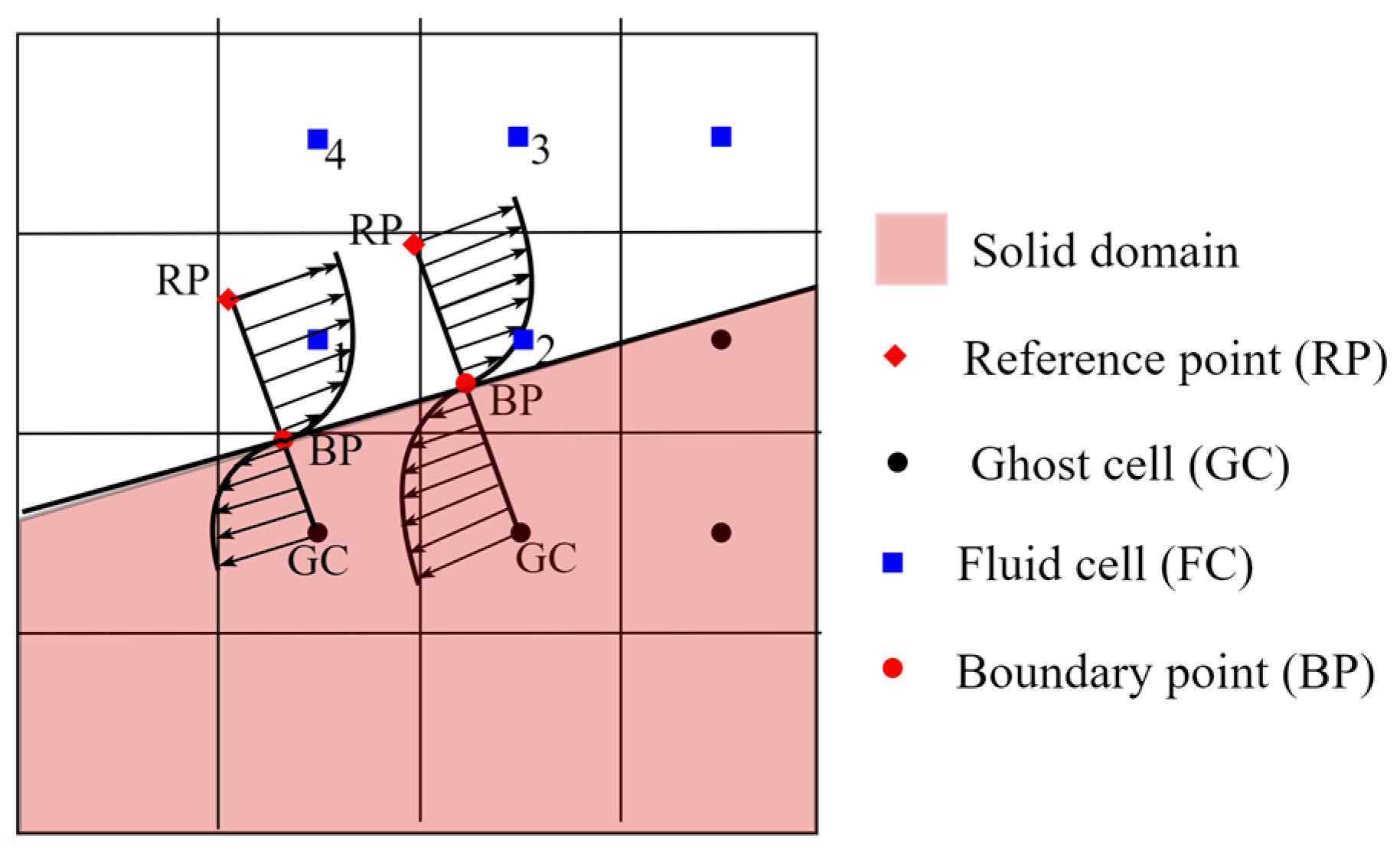
Then, the phase state of the background grid can be easily identified using the signed distance function of $\varphi$. The fluid cells (FCs) are those located in the fluid domain, the ghost cells (GCs) are located in the solid domain but adjacent to the fluid domain, and the solid cells (SCs) lie in the solid domain but exclude the ghost cells. Therefore, the ghost cells, the solid cells, and the fluid cells can be determined as follows:

1.

It is the GC, if ${\varphi }_{i,j,k}\le 0$ and (${\varphi }_{i\pm 1,j,k}>0$ or ${\varphi }_{i,j\pm 1,k}>0$ or ${\varphi }_{i,j,k\pm 1}>0$);

2.

It is the SC, if ${\varphi }_{i,j,k}\le 0$ and (${\varphi }_{i\pm 1,j,k}\le 0$ and ${\varphi }_{i,j\pm 1,k}\le 0$ and ${\varphi }_{i,j,k\pm 1}\le 0$);

3.

It is the FC, if ${\varphi }_{i,j,k}>0$ and (${\varphi }_{i\pm 1,j,k}>0$ and ${\varphi }_{i,j\pm 1,k}>0$ and ${\varphi }_{i,j,k\pm 1}>0$).

2.3. Immersed Boundary Wall Model

As the tangential velocity is highly nonlinear along the wall normal direction in the turbulent boundary layer, LES cannot capture the steep gradient and resolve the eddies accurately unless a very fine mesh is employed. Especially, in the Cartesian grid method, the wall gradients are substantially under-predicted on coarse grids. To reduce the requirement of the grid resolution for high Reynolds number near-wall flows, a linear interpolation for the velocity near the wall would be far from accurate. A near-wall treatment is needed to analyze near-wall turbulence. In this study, a wall model was devised to relieve the grid resolution in the near-wall region so that the near-wall grids could be coarser, so as to be related to the larger eddies developing in the fluid core. The basic idea is that the wall shear stress approximation is satisfied by the modified tangential velocity to make the near-wall computational cells remain in a numerically linear region.

To predict the wall shear stress, a reference point (RP) was introduced, obtained by mirroring the considered GC to the fluid domain. These reference points must not be too far from the wall to prevent them from being out of the boundary layer. A good compromise is to set the distance to the wall using $d_m=\sqrt{\Delta x^2+\Delta y^2+\Delta z^2}$. Figure 1 shows the near-wall treatment for the present immersed boundary method. Since the total wall shear stress near the wall is approximately constant, the wall shear stress at the ghost cell is set to be the same as that at the reference point. Assuming the total viscosity (the sum of molecular viscosity and eddy viscosity) of the ghost cell (GC) is identical to that of the reference point, the shear stress in the solver is approximated:

$${\tau }_w\approx \mu {\displaystyle \frac{V_{RP}-V_{GC}}{d_{RG}}}$$

(9)

where ${\tau }_w$ is the shear stress on the wall surface, d_RG is the distance from the reference point (RP) to the ghost cell (GC), and V_RP and V_GC are the velocities at the RP and GC, respectively. To correctly approximate the near-wall behavior, the law of the wall approximation is required to return the correct instantaneous wall–shear stress values corresponding to the known instantaneous velocity at the first node closest to the wall. It is assumed that the velocity profile near the wall obeys the law of the wall for a fully developed turbulent boundary layer. In general, the region close to the solid wall is divided into two sublayers in the wall function approach. It is known that Spalding’s formulation shows excellent agreement with various experimental data, even after y+ < 300; the wall function gives

$$y^{+}=u^{+}+e^{-\kappa B}\left[e^{\kappa u^{+}}-1-\kappa u^{+}-{\displaystyle \frac{{(\kappa u^{+})}^2}{2}}-{\displaystyle \frac{{(\kappa u^{+})}^3}{6}}\right]$$

(10)

where κ is the model coefficient, where κ = 0.41, B is the roughness parameter, where B = 5.0, assuming smooth blades, u⁺ is the dimensionless velocity with $u^{+}=u_t/u_{\tau }$, and $y^{+}$ is the dimensionless distance to the wall, where $y^{+}=y{u}_{\tau }/\upsilon$. $u_{\tau }$ is the friction velocity, and $u_t$ is the tangential velocity at the RP. The Newton–Raphson method is employed to solve Spalding’s law in Equation (10) for the friction velocity $u_{\tau }$, based on the tangential velocity sampled at the RP. The computed wall shear stress needs to be enforced in the governing equation. In the implementation of the wall function with near-wall coarse grid spacing, an incorrect velocity gradient and wall shear stress will be obtained when the no-slip condition is applied.

The pseudo-viscosity must be estimated near the immersed boundary. The eddy viscosity in Equation (3) is determined by the mixing length eddy viscosity model with near-wall damping.

$${\displaystyle \frac{{\upsilon }_t}{\upsilon }}=\kappa y^{+}{\left(1-e^{-y^{+}/A}\right)}^2$$

(11)

where A is an empirical coefficient, with A = 19. For a comprehensive review of the wall-modeled LES, the reader can refer to Bose and Park [39].

2.4. Actuator Line Model

In the ALM, each blade is simplified into a one-dimensional line, which is discretized spanwise into a series of actuator points (typically 20–30 points per blade), as illustrated in Figure 2. After obtaining the relative wind speed U_rel and angle of attack α at each actuator point, the corresponding lift coefficient C_L and drag coefficient C_D are obtained from airfoil lookup tables. The local lift force F_L and drag force F_D at each point are then calculated using blade element theory:

$$F_L = {\displaystyle \frac{1}{2}}\rho U_{rel}^{2}c{C}_L(\alpha )$$

(12)

$$F_D={\displaystyle \frac{1}{2}}\rho U_{rel}^{2}c{C}_D(\alpha )$$

(13)

where α is the angle of attack, U_rel is the local relative velocity of the fluid, c is the chord length, and C_L and C_D are the lift and drag coefficients of the airfoil, respectively. The angle of attack α, rotor inflow angle $\phi$, and relative velocity U_rel are essential for determining the lift and drag coefficients. These are computed as follows:

$$\alpha =\phi -\theta$$

(14)

$$\phi ={\tan }^{-1}\left({\displaystyle \frac{U_x}{U_{\theta }}}\right)$$

(15)

$$U_{rel}=\sqrt{U_{\theta }^2+U_x^2}$$

(16)

Here, θ is the pitch angle, defined as the angle between the chord line of the blade tip section and the rotor plane.

The computed lift and drag forces are then projected onto the surrounding fluid mesh nodes within a spherical region via a Gaussian projection function or a discrete Dirac delta function, resulting in a body force distribution. A projection radius of ϵ = 2.0Δx was selected to satisfy numerical stability. This body force term was subsequently incorporated into the Navier–Stokes equations for solution.

2.5. CPU-GPU Parallel Solver

To address the high resource demand and low efficiency of three-dimensional high-resolution simulations, this study establishes a CPU-GPU parallel framework to accelerate computations, with the program written in Fortran 90 in the CUDA (Compute Unified Device Architecture) environment. The hybrid CPU/GPU solution process is divided into two functional modules. The GPU undertakes core computing tasks to enhance parallelism and computational density, including the time advancement of the Navier–Stokes (N-S) equations, the processing of the immersed boundary, and the solution of the pressure Poisson equations. In contrast, the CPU only handles lightweight auxiliary tasks before and after time advancement, such as preliminary data preparation and post-computation result sorting. Furthermore, to optimize memory access efficiency, variables were allocated to different memory spaces (global memory, shared memory, and constant memory) based on their respective attributes and functional roles.

All simulations were executed on the Ubuntu 20.0 operating system with a Tesla A100 GPU. This GPU comes with 6912 CUDA cores and 40 GB of global memory. Additionally, the supporting Intel Xeon CPU is configured with 16 cores and runs at a processor clock rate of 3.2 GHz. In the two-dimensional oscillating cylinder case, this GPU parallel solver achieves a speedup ratio of hundreds of times compared with the corresponding serial solver. Furthermore, it achieves a speedup ratio of thousands of times in the three-dimensional oscillating cylinder case. For more in-depth technical details, the reader can refer to reference [37].

The implementation procedure of the present ALM-IBM parallel solver is briefly illustrated below.

(1) The complex geometry of a wind turbine is represented by the implicit iso-surface representation method in Section 2.2.

(2) The eddy viscosity coefficient, as well as the tangential and normal velocities near the wall, are reconstructed by the immersed boundary wall model in Section 2.3.

(3) Local velocities are sampled to compute the ALM blade forces in Section 2.4, which are projected onto the Eulerian grid.

(4) The N-S equations in Equations (1) and (2) are solved by using the added blade force.

3. Numerical Results

The proposed framework effectively combines the efficiency of the ALM with the geometric flexibility of the IBM. It overcomes the geometric simplification of the standalone ALM while avoiding the severe grid resolution in the IBM. Compared with the boundary element method (BEM), the present framework enables the capture of complex three-dimensional unsteady flow phenomena, such as massive separation or blade–vortex interactions. In addition, it eliminates the need for complicated grid regeneration, offering a significant efficiency advantage in comparison to the fully resolved body-fitted CFD method.

3.1. Flow Around a Three-Dimensional Cylinder

To validate the accuracy of the present near-wall turbulent model in the immersed boundary method, the flow around a three-dimensional cylinder at Re = 3900 was simulated. The computational domain spans 20D in the streamwise direction, with the inlet plane positioned 5D upstream of the cylinder center and the outlet plane 15D downstream of the cylinder center, where D is the diameter of the cylinder with D = 1 m. The spanwise (z) direction has a length of 5D, aligned with the cylinder axis, while the vertical (y) direction spans 10D, with the top and bottom boundaries each located 5D from the cylinder center and parallel to its cross-section. A steady uniform inflow velocity of U₀ = 1 m/s is imposed at the inlet. With a kinematic viscosity of ν = 1/3900 m²/s, the resulting Reynolds number based on the cylinder diameter is Re = U₀D/ν = 3900. A grid convergence study was conducted using two non-uniform grids. The first grid consists of 356 × 190 × 102 cells, with a uniformly spaced size in the spanwise direction. The grid is refined around the cylinder, with the minimum size of $\Delta x_{\min }$ = 0.016 and $\Delta y_{\min }$ = 0.016 along the x-y plane. The second, refined grid contains 476 × 236 × 102 cells, featuring enhanced resolution across critical regions, with the refined grid along the x-y directions.

To quantitatively examine the accuracy of the present method, the present results are compared with the reference results, as shown in

Table 1. Time-averaged results obtained by the present and reference methods.

Index	St Number	${\mathit{C}}_{\mathit{D},\mathit{a}\mathit{v}\mathit{g}}$
356 × 190 × 102	0.22	1.18
476 × 236 × 102	0.22	1.17
Lysenko [41]	0.19	1.18
Duan and Wan [40]	0.22	1.11
Lourenco and Shih [42]	0.21	1.04

. The St is a critical dimensionless number reflecting the vortex shedding frequency. When refining the grid from approximately 6.9 million cells (356 × 190 × 102) to 11.4 million cells (476 × 236 × 102), the Strouhal number (St) remains constant at 0.22, and the average drag coefficient (C_{D, avg}) changes by less than 1%, confirming good grid convergence. The predicted St of 0.22 aligns perfectly with Duan and Wan [40] and is very close to the widely accepted experimental and numerical range of 0.21–0.22. There is a notable discrepancy in the prediction of the mean drag force (C_{D, avg}) across different methods, stemming from the complex physics of the turbulent wake at Re = 3900. The flow is characterized by a laminar boundary layer separation, followed by a rapid transition to turbulence in the shear layers. It possesses rich three-dimensional structures, highlighting its sensitivity to physical parameters.

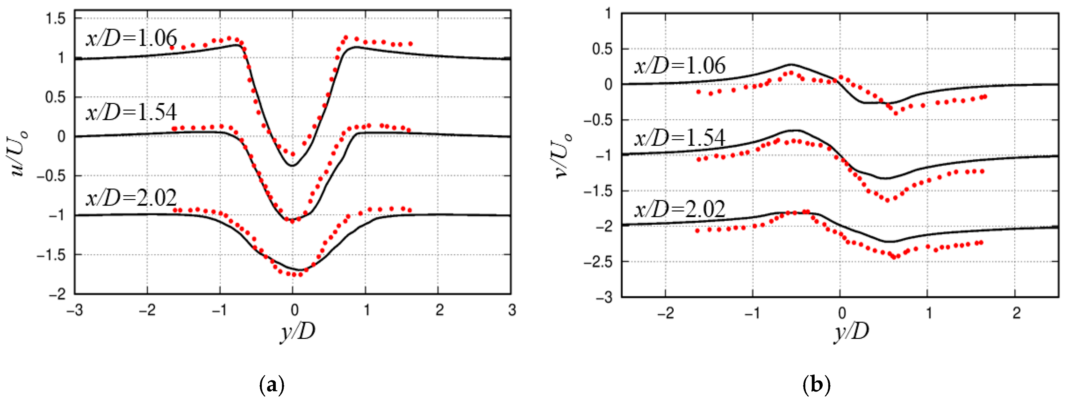
To quantitatively examine the local flow structures, Figure 3 illustrates the mean streamwise and cross-wise velocities at different locations in the wake region; the lines represent the present results, and the symbols are the experimental results by Lourenco and Shih. In Figure 3a, the profiles exhibit the classic “W” shape characteristic of a time-averaged vortex street. This consists of a significant velocity deficit at the centerline (y/D = 0) and two local velocity maxima on either side. As the flow moves downstream (from x/D = 1.06 to 2.02), the wake undergoes a recovery process: the centerline velocity deficit becomes less pronounced, the wake widens, and the velocity peaks diminish. In Figure 3b, the profiles of the cross-wise velocity are anti-symmetric about the centerline, showing a mean flow directed inwards towards the center of the wake. This inward motion is a direct consequence of the low-pressure region behind the cylinder, which forms the core of the mean recirculation bubble. As the flow moves downstream, the magnitude of this inward velocity decreases, indicating the gradual closure of the recirculation bubble and the recovery of pressure. The present simulation captures this overall topology. However, a minor discrepancy with Lourenco and Shih [42] is visible. The present u/U₀ predicts a deeper and narrower deficit than the experiment. At every x/D location, the black line at y/D = 0 is below the red experimental points. Moreover, the present v/U₀ tends to predict a slightly larger magnitude of the cross-wise velocity compared to the experiment, especially at x/D = 1.54 and 2.02. The local velocity discrepancies in Figure 3 are a direct and consistent consequence of the global drag force discrepancy noted in Table 1. This can be attributed to a slight under-prediction of turbulent evolution in the immediate near-wake. The entrainment of high-momentum fluid into the wake center is delayed if the shear layer instabilities are not fully resolved at the subgrid level in LES, leading to a deeper profile. Further, the current grid resolution in the spanwise direction, while sufficient for capturing global forces, may slightly dampen these fine-scale shear layer instabilities. Consequently, the wake remains more coherent and narrow compared to the experiment.

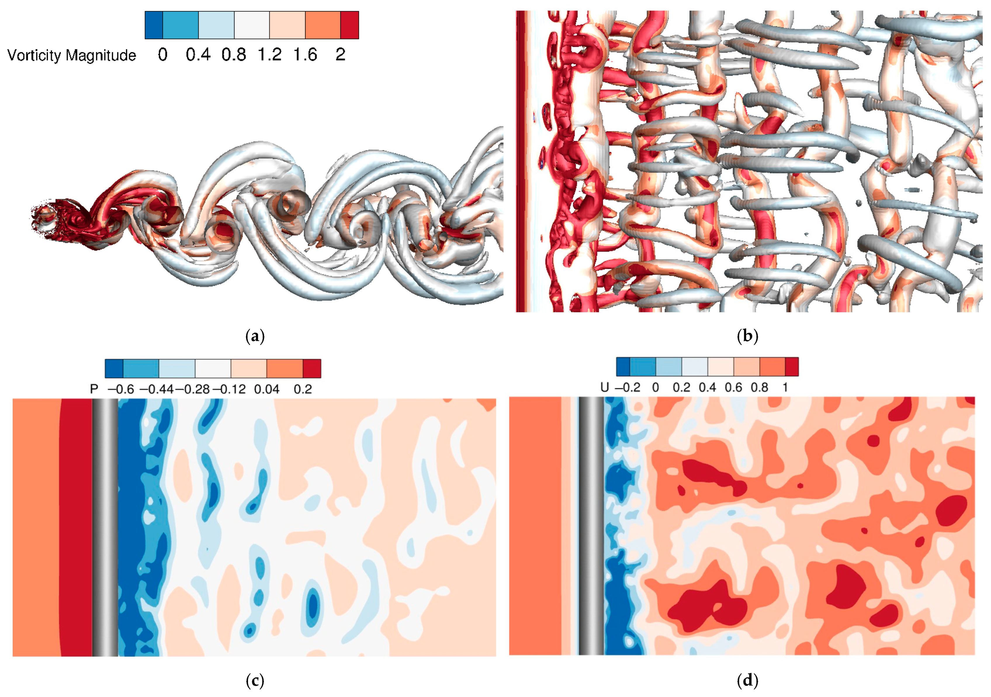
Figure 4 provides an instantaneous snapshot of the complex, three-dimensional vortex dynamics in the wake of the cylinder at Re = 3900. In Figure 4a, we see large-scale, coherent “rollers” being shed alternately from the top and bottom of the cylinder. These primary vortices form, grow, and then begin to lose their coherence as they travel downstream, breaking down into smaller, more chaotic turbulent structures. The coloring by vorticity magnitude highlights the intense rotational motion within the vortex cores and the shear layers separating from the cylinder. We can clearly see streamwise “rib” vortices connecting the primary rollers and vortex loops that cause significant distortion along the span, as shown in Figure 4b. The streamwise rib vortices and loops locally alter the flow, creating pockets of low pressure and modifying the velocity field in Figure 4c,d. This intricate “braid” of vortices is the hallmark of a transitional turbulent wake and secondary instabilities.

3.2. Aerodynamic Performance for a Fixed-Type Turbine

To accurately compute the aerodynamic loads on a wind turbine, this section shows unsteady computations for the fixed-bottom configuration without platform motion. The NREL 5 MW offshore wind turbine was adopted, which was developed by the National Renewable Energy Laboratory (NREL). The installation and motion parameters of the NREL 5 MW turbines are provided in

Table 2. Installation and motion parameters of NREL 5 MW turbines.

Parameters	Values
Number and diameter of blades Hub diameter	3, 126 m 3 m
wind speed	4, 6, 8, 10, 11.4 m/s
Rotational speed	7.18, 7.94, 9.16, 11.43, 12.1 rad/s
Tilt angle, precone angle	5°, 2.5°
Blade pitch angle	13.308°

. The hub center of the wind turbine rotor is defined as the origin of the Cartesian coordinate system. The x-axis is aligned with the downwind direction, the z-axis is oriented along the radial direction of a reference blade, and the y-axis is determined by the right-hand rule. 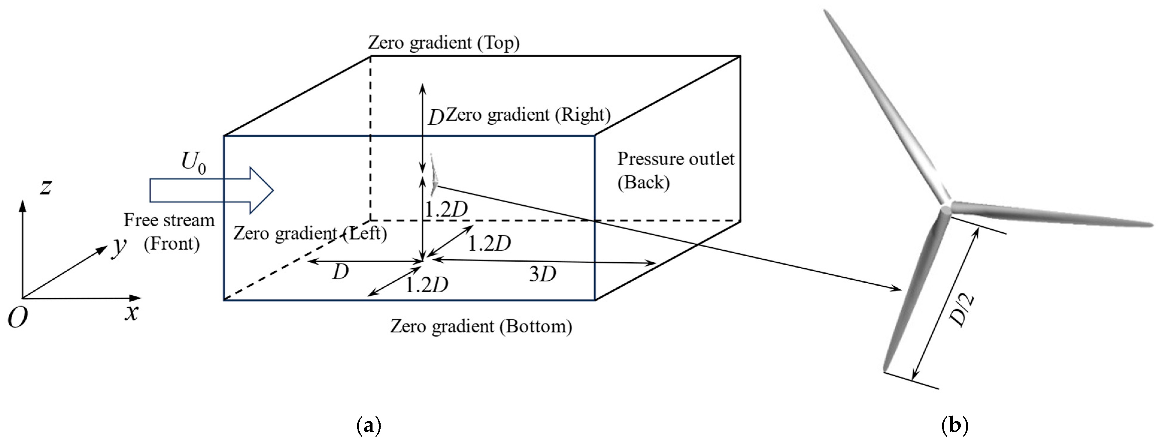The computational flow domain is defined as a rectangular volume extending 1.5D upstream and 3D downstream of the origin, where D is the diameter of the cylinder at D = 126 m. The computational domain and the geometry of the wind turbine are shown in Figure 5. The turbined surface is represented in a Lagrangian way by 54,228 triangular elements. For the boundary conditions, a velocity inlet is enforced upstream of the turbines, where the inflow velocity U_∞, and v = w = 0, with U_∞ set to the wind speed. A pressure outlet is positioned 3D downstream of the turbines, where the relative static pressure is set to zero. Symmetry boundary conditions are applied to the top, bottom, and side faces of the domain, all located 1.5D from the turbines.

To validate the accuracy and reliability of the present ALM and near-wall turbulent model for wind turbines, the rated wind velocity was set to U_∞ = 11.4 m/s, and the rotational velocity was set to 12.1 rad/s. To examine grid convergence, three non-uniform Cartesian grids were adopted.

Table 3. Detailed information for three grids for wind turbines.

Index	Grid Number	Minimum Sizes
Grid #1	232 × 204 × 204	0.60 × 0.80 × 0.80
Grid #2	310 × 238 × 238	0.43 × 0.70 × 0.70
Grid #3	386 × 300 × 300	0.30 × 0.54 × 0.54

shows the detailed information of the three grids, from a coarse grid (#1) to a fine grid (#3). The symbol ‘#’ denotes the grid number. Grid #1, #2, and #3 correspond to the coarse, medium, and fine mesh resolutions, respectively. The computational domain is refined around the turbines at an area of [−0.1D, 0.8D] × [−0.55D, 0.55D] × [−0.55D, 0.55D] in the x-, y-, and z-directions, respectively. Correspondingly, the minimum grid sizes for the coarse grid in three directions are $\Delta x_{\min }=0.6$, $\Delta y_{\min }=0.8$, and $\Delta z_{\min }=0.8$. The time step was set to Δt = 0.0001 s based on the Courant–Friedrichs–Lewy (CFL) condition. It ensures numerical stability while providing sufficient temporal resolution to capture transient wake structures.

Table 4. Comparison of computed results obtained with three distinct grids against predictions from STAR-CCM+ and FAST.

Method	Thrust/kN	Torque/kN·m
Grid #1	646	4145
Grid #2	649	4136
Grid #3	650	4130
STAR CCM+ [41]	693	4085
FAST	713	4194

presents the thrust (F_N) and the torque (F_Q) calculated by the present method on three grids. Moreover, the results obtained by STAR CCM+ [43] and FAST are added for comparison. The present thrust (F_N) and torque (F_Q) for the three grids are close. Especially, the errors of the thrust and torque on the two finer grids of #2 and #3 are within 1%, confirming satisfactory grid convergence. To balance efficiency and accuracy, the medium grid of #2 was adopted in the following calculations. In addition, the present results show good agreement with the reference results. For example, the error of the thrust between grid #2 and STAR-CCM+ is 6.3%, and it is 1.2% for the error of the torque, demonstrating the accuracy of the present method.

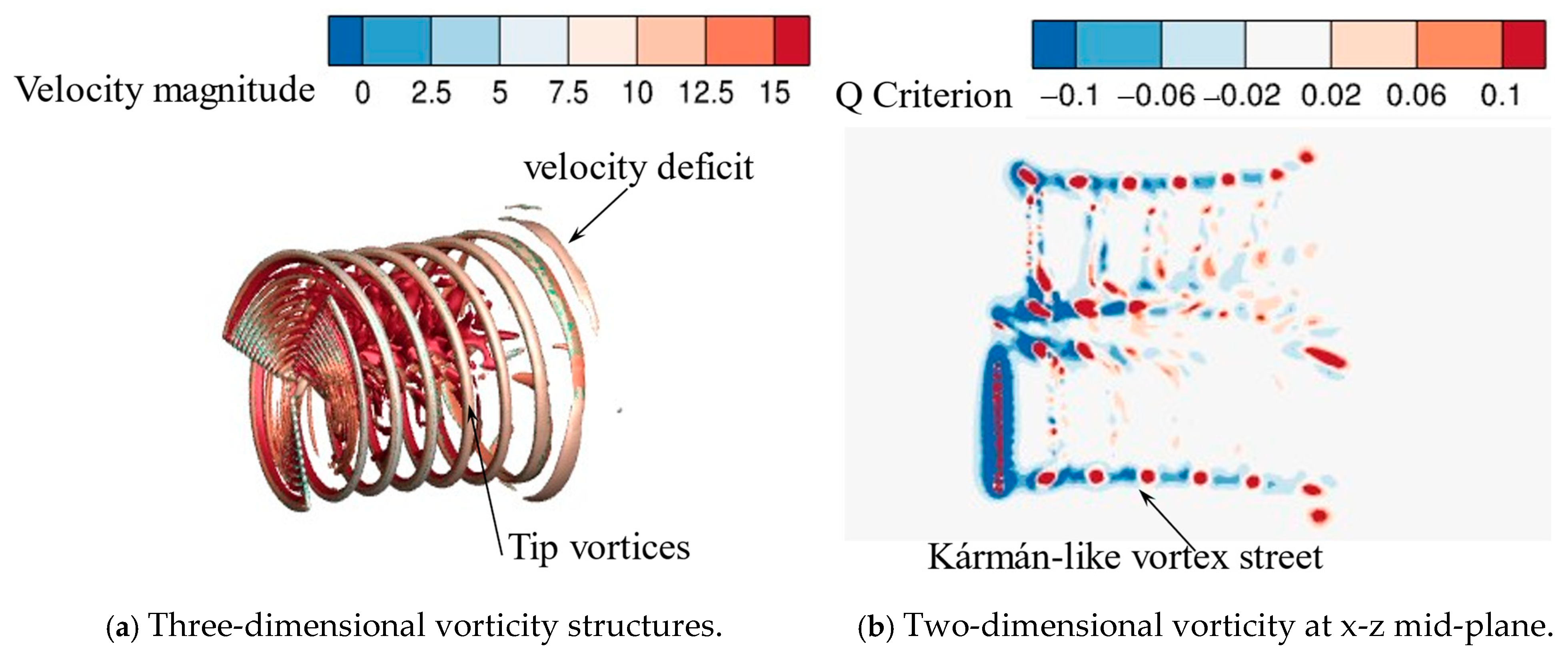
To reproduce the wake structures, Figure 6 provides an instantaneous visualization of the wake generated by a fixed-bottom wind turbine. It reveals a complex, three-dimensional, and evolving vortex system that is the direct fingerprint of the turbine’s operation. In Figure 6a, the three-dimensional vortex structure exhibits distinct spiral wake vortices, which shed from the blade tips, forming tip vortices that gradually break down and entangle downstream, eventually evolving into a turbulent wake. The colored velocity magnitude shows a significant velocity deficit in the wake region, with the maximum deficit located in the near-wake region, gradually recovering with increasing downstream distance. In Figure 6b, the two-dimensional vorticity slice (right panel) clearly shows a distinct pattern in the center of the wake, directly behind the tower (represented by the black line). This pattern consists of larger, alternating patches of positive and negative vorticity, characteristic of a bluff body wake similar to a Kármán-like vortex street. These vortex structures interact downstream, resulting in vortex pairing and vortex breakdown.

3.3. Aerodynamic Performance at Different Operating States

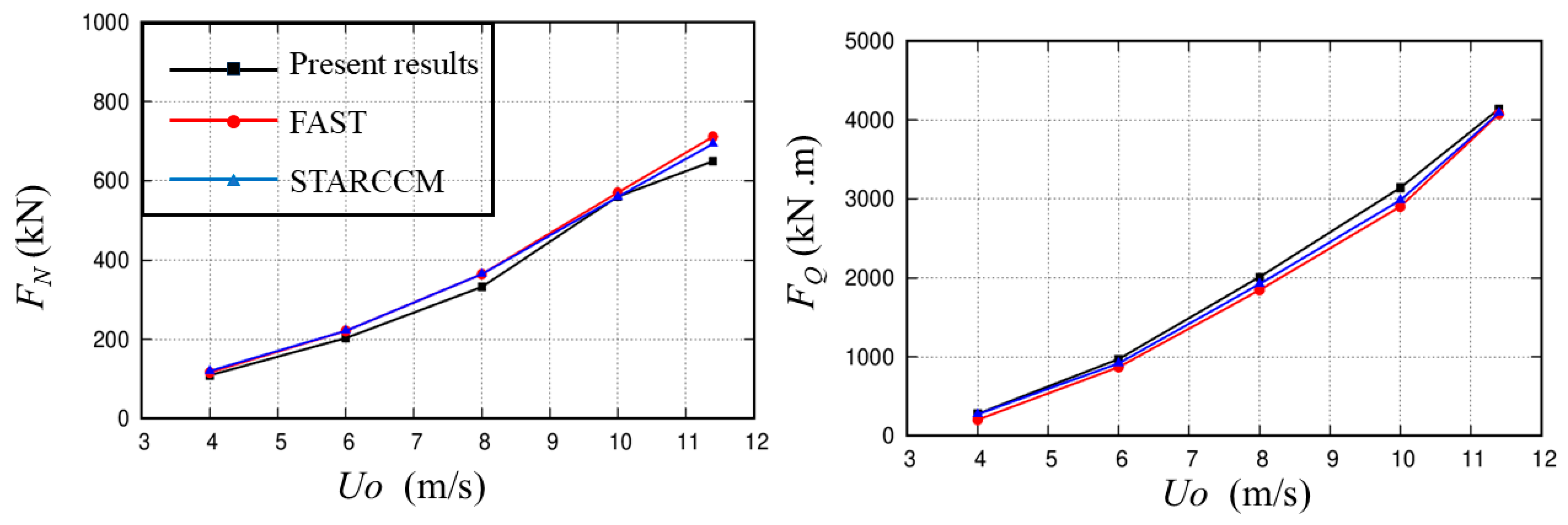
To further investigate the aerodynamic performance of the wind turbines under different operating states, we further simulated uniform flow around rotating wind turbines under different inlet and rotational velocities. Figure 7 displays the variation of the thrust (F_N) and torque (F_Q) with incoming wind speed (U_∞) when operating below the rated wind speed. Moreover, the results calculated by FAST and STARCCM [43] are provided for comparison. The two curves clearly demonstrate that both thrust and torque exhibit a nonlinear, accelerating increase with rising wind speed, which approximates a quadratic dependence. Furthermore, the three distinct numerical models show a high degree of consistency in predicting global performance. Although the three models generally agree well, the minor discrepancies among them reveal the differences in the capabilities of various numerical methods in capturing complex physical phenomena. The present results are slightly lower than those of FAST and STAR-CCM+ in terms of thrust due to Gaussian force projection. This numerical dispersion effect smoothens the pressure peaks on the blade surface. It may lead to a slight reduction in the resolved tip vortex intensity, collectively manifesting as a mild decrease in the integrated thrust. The minor differences between FAST and STAR-CCM+ may stem from the simplification of three-dimensional flow in the boundary element method (BEM) compared to the high-fidelity simulation of CFD.

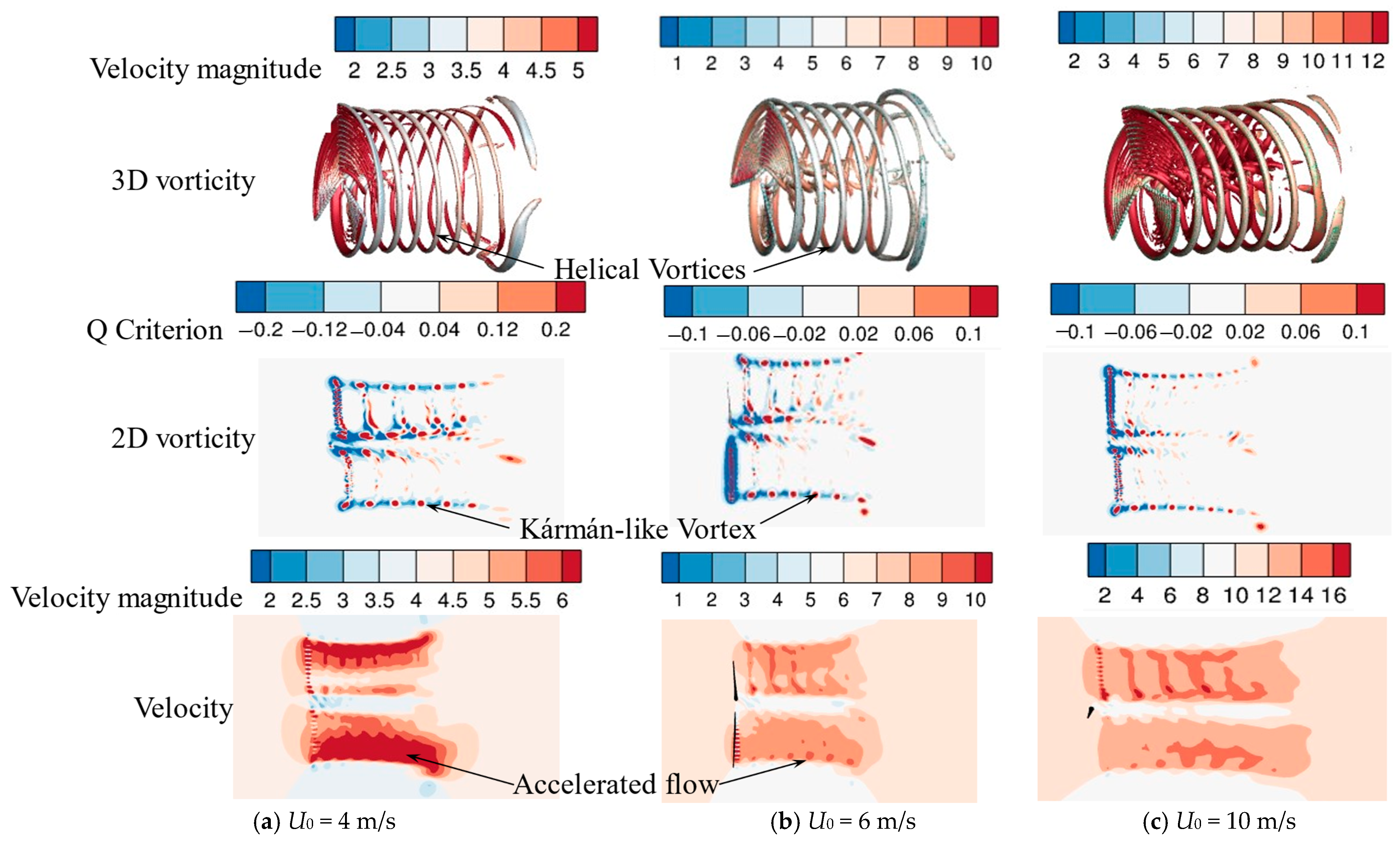
Figure 8 presents a multi-faceted view of the fluid dynamics around a wind turbine rotor under three distinct incoming wind velocities: 4 m/s, 6 m/s, and 10 m/s. The three-dimensional large-scale vortical structures are visualized in the wake using the Q-criterion, colored by velocity magnitude. The dominant feature is a system of intertwined, stable helical vortices, originating from the tips and roots of the rotating blades. As the wind speed U₀ increases from 4 m/s to 10 m/s, the pitch of the helical vortices decreases, meaning the helices become more tightly wound. The wake also appears to undergo a more significant radial expansion at higher wind speeds. In Figure 8b, the cross-sections of the three-dimensional helical structures are reproduced. The distinct, alternating patches of the vortex tubes are shed from the trailing edges of the blades. As U₀ increases, the strength and complexity of the shed vorticity increase. The wake becomes more turbulent and less organized further downstream, indicating a faster breakdown of the coherent vortex structures. In Figure 8c, the primary feature is the velocity deficit in the wake. We can observe regions of accelerated flow around the edges of the wake, particularly near the blade tips. The velocity deficit becomes dramatically more pronounced as U₀ increases. At 10 m/s, the velocity in the near wake is significantly lower relative to the incoming flow compared to the 4 m/s case. The wake is also wider and persists for a longer distance downstream.

4. Conclusions

This study presents a hybrid numerical framework designed by combining the wall-modeled Immersed Boundary Method (IBM) with an actuator line method (ALM) to address the enduring challenge of balancing accuracy and computational cost in wind turbine aerodynamics. This synergistic approach leverages the strengths of each component: the IBM accurately resolves the complex, near-wall turbulent flows around non-blade components like the tower, while the ALM efficiently models the aerodynamic forcing of the rotor blades.

The robustness and fidelity of the numerical model were rigorously established through two key validation cases. First, the simulation of flow over a three-dimensional cylinder at a Reynolds number of 3900 yielded excellent agreement with experimental data and previous numerical studies. The model accurately predicted the Strouhal number (St = 0.22) and captured the intricate three-dimensional vortex dynamics and mean flow recovery in the wake, confirming the efficacy of the IBM and the implemented near-wall turbulence model.

Subsequently, the framework was applied to the NREL 5 MW offshore wind turbine model. The simulations demonstrated strong predictive capabilities, with calculated thrust and torque values showing good agreement with established benchmark data from FAST and STAR-CCM+ across a range of sub-rated operating conditions. Beyond integral loads, the high-fidelity LES approach provided detailed insights into the complex wake physics. It successfully visualized the formation, helical structure, and eventual breakdown of the tip and root vortices, as well as the distinct bluff body vortex shedding from the tower. The analysis of different wind speeds clearly illustrated the physical response of the wake, showing how the helical vortex pitch and velocity deficit evolve with operational changes.

The present framework is suitable for hydrodynamic applications involving rotating blades within complex geometries. For example, it can be applied to the energy harvesting of tidal stream turbines and marine propeller propulsion when integrating specific physical sub-models (e.g., free surface capturing model). However, the accuracy of the present framework would be compromised for predicting the viscous sublayer for extremely high Reynolds numbers, compared to body-fitted simulations. Furthermore, this study focused on uniform inflow. In the near future, we expect to extend the present model to the simulations of turbulent inflow.