Article

Analysis of the Multi-Scale Spatial Heterogeneity of Factors Influencing the Electric Bike-Sharing Travel Demand in Small and Medium-Sized Cities

1
College of Automobile and Traffic Engineering, Nanjing Forestry University, Nanjing 210037, China
2
Department of Geography, Virginia Tech, Blacksburg, VA 24061, USA
3
Department of Geography, Kyung Hee University, Seoul 02447, Republic of Korea
4
Department of Climate-Social Science Convergence, Kyung Hee University, Seoul 02447, Republic of Korea
5
Department of Convergence and Fusion System Engineering, Kyungpook National University, Sangju 37224, Republic of Korea
6
Division of Computational Social Science, School of Humanities and Social Science, The Chinese University of Hong Kong, Shenzhen (CUHK-Shenzhen), Longgang District, Shenzhen 518172, China
*
Author to whom correspondence should be addressed.
Sustainability 2025, 17(23), 10437; https://doi.org/10.3390/su172310437
Submission received: 17 October 2025 / Revised: 13 November 2025 / Accepted: 19 November 2025 / Published: 21 November 2025

Abstract

The spatial heterogeneity of the electric bike-sharing (EBS) travel demand in small and medium-sized cities is influenced by a combination of the built environment, socio-economic gradients, transportation accessibility, and residents’ travel behavior patterns, and is significantly different from the shared travel characteristics of developed cities. In order to explore the influencing mechanisms of the EBS travel demand under different travel distance scales in small and medium-sized cities, this paper utilizes multi-source data from Tongxiang, Zhejiang Province, including operational data of EBS and built environment data. This paper analyzes the impact of the built environment on the EBS travel demand and its spatial heterogeneity across various distance scales from a local perspective. The results demonstrate that the fit of the multiscale geographically weighted regression (MGWR) model is superior to that of the geographically weighted regression (GWR) and the ordinary least squares (OLS) model. The explanatory variables exhibit significant spatial heterogeneity in their influence on the demand for EBS trips across different distance scenarios. The density of primary roads demonstrates a positive correlation with EBS travel demand in the western urban core area, but it is negatively correlated with travel demand in the eastern urban core area. Accommodation services show a negative correlation with long-distance EBS travel demand in the urban core area and the northern city, but they are positively correlated with short-distance EBS travel demand in the urban core area. There is competition between long-distance EBS and public transportation in city centers. However, short-distance EBS and public transportation exhibit a complementary relationship in the urban periphery. The research findings are beneficial for gaining a deeper understanding of the patterns of change in the EBS travel demand and promoting the refined and sustainable development of shared transportation.

1. Introduction

Urban transportation is a significant source of energy consumption and greenhouse gas emissions and is also a critical area for urban environmental pollution and for promoting sustainable development. In the context of increasing global pressure to reduce carbon emissions, urban transportation systems are rapidly transitioning toward greener, low-carbon models, and there is a broad consensus that electric bike-sharing (EBS) can ease urban traffic congestion while achieving energy savings and emission reductions [1]. As a new travel mode, EBS has become a frequent choice for many urban residents because of its many features, such as low cost, flexibility, convenience, and low carbon emissions. Statistics from the China Urban Public Transport Association show that, by July 2024, more than 300 cities across the country had launched EBS services, with over 15 million e-bikes in operation and more than 200 million users, generating tens of millions of orders per day. EBS not only helps to alleviate urban traffic congestion but also effectively complements the insufficiencies of public transportation accessibility, making it an important mode of transport for short-distance travel. At the same time, it significantly encourages and promotes green travel among urban residents and helps to address urban motorization issues.
EBS’s development modes and demand characteristics in small and medium-sized cities show outstanding differences compared to those in large cities. For example, existing studies have shown that in Qujing city, compared with Kunming city, the travel distance is shorter, and the usage rate of public transportation is lower. Residents in remote areas still rely heavily on private cars to meet long-distance travel needs, while electric bicycles play an important role in both local and regional travel [2]. Unlike large cities, which have well-developed infrastructure, dense road networks, and mature transportation systems, small and medium-sized cities often exhibit a monocentric sprawling pattern. Although the urban areas continue to expand outward, functional zones such as employment, commerce, and residential areas are distributed sparsely, and the demand for medium-to-short-distance travel is prominent. Meanwhile, transportation facilities, public transit accessibility, and income levels are relatively low, making EBS a major choice for short-distance travel [3]. This results in the EBS demand showing a spatial differentiation pattern compared to that in traditional developed cities. Small and medium-sized cities are characterized by small spatial scales, single-center agglomeration, close work–residence relationships, and convenient commuting [4,5]. In contrast, developed cities often have multiple urban centers with high degrees of land use mixing, where a single area can integrate multiple functions such as work, residence, commerce, entertainment, education, and healthcare [6,7]. Moreover, the continuous expansion of small and medium-sized cities has exacerbated the supply and demand imbalance of EBS. From the perspective of travel distance scale, the demand for short-distance ECS trips tends to cluster in the city center and is more likely to replace bicycles and walking. In contrast, the demand for longer-distance trips is scattered in the peripheral areas of the city, leading to a loss of passenger flow from traditional taxis and public transportation. Therefore, the travel characteristics of EBS in small and medium-sized cities and the impact mechanisms of the built environment on their use cannot directly draw on the research conclusions of EBS travel in large cities. However, the vast majority of current studies on the impact of the built environment on the EBS demand focus on large or developed cities. Due to the essential differences in spatial structure, transportation systems, and travel behavior between small and medium-sized cities and large cities, the research conclusions from large cities are difficult to directly apply and promote. More importantly, the impact of the built environment on the EBS demand may exhibit significant spatial heterogeneity. How this heterogeneity is specifically manifested at different travel distances remains a key issue that has not been fully explored in the context of small and medium-sized cities, forming an important research gap.
This paper aims to reveal the influencing factors and spatial heterogeneity of the EBS travel demand in small and medium-sized cities under different travel distance scales. Compared with existing studies, the innovations and contributions of this research are mainly reflected in the following three aspects: (1) Based on the actual operation order data of EBS in Tongxiang City in July 2024, the travel data is clearly divided into long-distance and short-distance groups using the median of riding distance (1.66 km) as the threshold, and the demand characteristics and influencing mechanisms of each group are explored separately. Not only does this ensure the balance of sample size, but more importantly, it effectively distinguishes the rigid long-distance demand mainly for commuting and the elastic short-distance demand mainly for short-distance connection, providing a methodological basis for accurately identifying the key driving factors of various travel demands. (2) Current shared travel studies mostly focus on large or developed cities, and their conclusions are difficult to directly apply to small and medium-sized cities, which have significant differences in spatial structure, transportation facilities, and development stages. Taking Tongxiang City, a typical small and medium-sized city, as a case, this paper systematically reveals the EBS travel patterns under the characteristics of its monocentric structure, close job–residence relationship, and the public transportation system still in development. It can provide refined deployment strategies for EBS companies in other small and medium-sized cities, help improve service efficiency and optimize corporate operation strategies. (3) The MGWR model is adopted to overcome the limitations of traditional OLS and GWR models, allowing different variables to play their roles at their optimal spatial scales, thereby more accurately identifying the key influencing variables affecting the EBS travel demand.

2. Literature Review

2.1. Characteristics of the EBS Travel Demand Based on Questionnaire Surveys

Utilizing the data obtained from questionnaires surveys to analyze the EBS and bike-sharing (BS) travel behavior, this method can analyze travel patterns from the perspectives of user characteristics, travel purposes, and psychological preferences. Tang et al. [8] constructed structural equation models for the E-TPB and the O-TPB based on a self-reported survey of over 2000 EBS users in Shanghai. The model results indicate that the willingness of riders to violate traffic regulations and their accident proneness are influenced by descriptive norms, conformity tendencies, and past behavior. Li et al. [9] examined the willingness of residents in Meizhou, a small and medium-sized city, to use EBS based on the extended theory of planned behavior. The analysis of data from 751 respondents shows that personal attitudes, subjective norms, and perceived behavioral control all have significant positive effects on the intention to use it. Li et al. [10] constructed a structural equation model based on online survey data from 313 EBS users in Ningbo. The results indicated that over 60% of users utilized EBS during morning and evening rush hours. Additionally, 69.33% of the orders had travel distances between 1 km and 4 km, with an average travel distance of 3 km. Campbell et al. [11] established a polynomial logistic regression model based on 623 survey data entries from Beijing. The study revealed that BS is primarily used for short-distance travel, while EBS is more suitable for medium- to long-distance travel. The travel characteristics of EBS are closer to those of private electric bicycles. The user group mainly consists of young to middle-aged men, and users with low income and low education levels are more inclined to use EBS for travel. Chen et al. [12] classified users using the K-means clustering method based on 624 survey questionnaires from Nanjing. They investigated the attitudes and behavioral characteristics of Nanjing residents towards dockless BS. The results showed that the main reasons for users choosing BS are the convenience of picking up and returning bikes, easy payment, and low cost. Additionally, users have a strong demand for adding parking areas around subway stations and residential communities. Yang et al. [5] used 500 survey questionnaires from Xuchang to explore the travel characteristics of BS in small and medium-sized cities. The analysis pointed out that due to the small city size and simple road conditions, a high proportion of short-distance travel by residents leads them to choose BS instead of walking or private bicycles, making BS one of the main commuting modes in small and medium-sized cities. Li et al. [13] used a binary logistic model to study the factors influencing BS travel behavior based on 30,401 valid questionnaires from Nanjing. Their results indicated that the travel demand gradually decreases from the city center to suburbs, while the demand increases significantly in areas with a high concentration of universities. Studies based on surveys generally analyze travel characteristics of shared micro-mobility from environmental conditions, user demographics, and travel attributes, but fail to consider the impact of the built environment on travel factors. Ning et al. [14] conducted a study to explore the differences in the choice preferences for bicycle-sharing modes between urban and suburban travelers. They collected 810 valid questionnaires in Nanjing and established random parameters logit models based on the data. The study found that the riding distance is the key factor dominating the choice: for connections within the range of 800–1500 m, BS are the preferred choice; while for connections within the range of 2500–4000 m, travelers are more inclined to use EBS, a phenomenon that is particularly evident in suburban areas.

2.2. Spatial Heterogeneity Analysis of Micro-Mobility Travel Based on Multi-Source Data Sharing

Analyzing the influencing factors and spatial heterogeneity of the BS travel demand through multi-source data can effectively quantify the impact of factors such as road infrastructure, the built environment, and urban structure, providing a comprehensive understanding of their effects on travel behavior. He et al. [15] established a Poisson regression model based on historical travel data from EBS in Park City, Utah. Their study found that in tourist cities, young people, middle-aged people, and tourists are more likely to use EBS. In addition, entertainment venues and sightseeing are the main purposes of using EBS, rather than commuting to work. Li et al. [4] used kernel density models and spillover commuting models for analysis based on the real-time GPS data of EBS in Tengzhou city. The research results indicated that areas with bus terminals, city squares, and government institutions were positively correlated with the use of EBS. In contrast, rural areas were negatively correlated with the use of EBS. Based on the trip data of EBS in Zurich, Guidon et al. [16] used a spatial autoregressive model to explore the impact of spatial characteristics on the demand for EBS. The results showed that the demand for EBS trips was positively correlated with population density, bus stop density, and workplace density. Moreover, areas with a high concentration of bars and restaurants significantly increased the demand for trips during the night and on weekends. Ma et al. [17] analyzed the differences in travel characteristics between docked and dockless BS systems using order data, population density, and GDP. The results showed that dockless bicycles have a higher usage rate in the city center, while docked bicycles are more concentrated in the western part of the city where docking stations are densely located. Lang [18] analyzed the impact of BS on public transportation using BS order data, bus passenger data, and points of interest (POIs) data. The study found that within a 3 km travel range, users tend to choose BS as an alternative to buses, with the substitution willingness gradually decreasing as the distance increases. Shi et al. [19] constructed a geographically and temporally weighted regression model using one month of EBS order data from Kunming. Their study found that the number of leisure and entertainment POIs was positively correlated with the usage rate of EBS throughout the day. During the morning peak period, the EBS usage in areas with company and business distributions showed significant increases, and residents living closer to work areas were more likely to use EBS for short-distance commuting.
To further examine the spatial heterogeneity of influencing factors, scholars have begun to study shared micro-mobility by building geographically weighted regression models. Gou [20] used GWR, GTWR and MGWR models to study the impact of the built environment on the passage of EBS. The results showed that government institutions have a positive impact on EBS travel during non-peak hours, while entertainment and leisure venues only significantly affect travel during morning peak hours. Bus stops showed a positive correlation with EBS travel only during the morning peak period. Zhu et al. [21] developed a new model framework that integrates XGBoost and GTWR to address the issue of ignoring spatiotemporal heterogeneity in machine learning methods. Taking Hefei City as an example, they used the integrated model to study the impact of the built environment on the travel of BS and EBS. The results show that the demand for BS use is mainly concentrated in the urban area, while the demand for EBS use is more evenly distributed throughout the city. Chen [6] constructed GWR and MGWR models to analyze the order data from BS and EBS in Manhattan, New York City. The study found that for travel distances over 2 km, the proportion of users choosing EBS was significantly higher than for BS. Additionally, areas with concentrations of commercial and financial facilities promoted the demand for shared travel, while areas with dense cultural facilities suppressed the use of shared services. Bus stations had a more significant positive impact on EBS than on BS. Li et al. [7] constructed OSL and GWR models to explore how the built environment and population characteristics affect the use of BS. The results showed that public transportation stations, population density, POI mix, and commercial and residential areas significantly promoted the demand for BS. Tang et al. [22] established a cross-city GWR model to study the impact of the built environment on the travel demand of BS. The results showed that travelers preferred to ride BS to restaurants, parks, shopping centers, and other leisure areas. The impact of specific points of interest such as financial institutions, government agencies, and medical services on the travel demand varied significantly due to differences in infrastructure, population density, and cultural factors among cities.
In summary, scholars have conducted some research on EBS travel behavior characteristics and their influencing factors and have begun to focus on how the built environment affects the EBS travel demand. However, existing research has obvious regional limitations. On one hand, studies are mainly concentrated in developed or specific first-tier cities, whose road facilities, urban structure, resident travel behaviors, and travel habits differ from those in small and medium-sized cities, making it difficult to fully apply the research results. On the other hand, research has not yet explored travel demand across different spatial scales, and the factors affecting short- and long-distance travel have certain differences in their spatial scope of influence. Based on this, this paper relies on multi-source data from Tongxiang City to reveal the influencing factors of the EBS travel demand at different distance scales, both globally and locally. First, OLS and GWR models are used to identify the significant explanatory variables that affect travel demand. Then, a multi-scale geographically weighted regression (MGWR) model is used to analyze the influencing factors of travel demand at different distance scales and their spatial heterogeneity. The research results will provide theoretical insights for achieving supply–demand balance for EBS at different distance scales in small and medium-sized cities.

3. Data

3.1. Survey Area

Tongxiang City is located in the northern part of Zhejiang Province with a very advantageous geographical location. It is situated 131 km to the east of Shanghai, 74 km to the north of Suzhou, and 65 km to the west of Hangzhou, within the economic circles of Shanghai, Hangzhou, and Suzhou. The total area of Tongxiang City is 727 km2, which includes eight towns and three sub-districts under its jurisdiction (Figure 1). The registered population of Tongxiang City is 721,600 people. According to data from the People’s Government of Tongxiang City in 2025, the GDP of Tongxiang City in the first half of the year was 65.754 billion yuan. Tongxiang City is a county-level city under the administration of Jiaxing City. Among the counties and districts under the jurisdiction of Jiaxing City, Tongxiang City ranks second in economic output, indicating that it is an important and economically active county-level city. Its superior administrative unit, Jiaxing City, is a prefecture-level city of medium standing in Zhejiang Province, ranking fifth in GDP among the 11 prefecture-level cities in Zhejiang Province. Typically, developed cities have a tertiary industry that accounts for more than 70% of GDP. However, data from the People’s Government of Tongxiang City shows that the proportion of the tertiary industry in Tongxiang City’s GDP is only 54.3%. Therefore, there is a significant difference between Tongxiang City’s GDP and that of developed cities. According to the data from 2024, Tongxiang City has a total of 35 urban bus routes, 4000 public bicycles in operation within the city, 8000 e-bikes deployed, and an average daily rental volume of over 27,000. This indicates that EBS occupies a vital and important position in the local transportation system and in residents’ travel modes. In addition, the region currently does not have a rail transit system. Tongxiang city has not yet met the criteria of developed cities, and its characteristics can be more widely applied to the many emerging prefecture-level or county-level cities in China with similar patterns, avoiding the bias brought by the particularity of extreme cases. Therefore, conducting research on EBS in this area has great reference value for understanding shared travel in small and medium-sized cities.

3.2. Data Processing

The data were obtained from the operation order data of EBS in Tongxiang City in July 2024, including the order ID, vehicle number, latitude and longitude coordinates of the origin and destination, the start and end times of the order, and the travel distance. The data were filtered by vehicle type, and orders with abnormal data, such as a travel distance of 0, were removed, as well as orders involving vehicle return failures. After data preprocessing, there were 214,355 valid records.
In order to analyze the influencing factors of EBS travel demand, multi-source data for the study area were collected, including road networks, population, and POI (Points of Interest) data. The road network data were obtained from the historical data of OpenStreetMap, which has been used in previous studies to quantify road-related elements and has demonstrated good reliability [23]. The population data are derived from the 2023 China Population Grid Database provided by the Oak Ridge National Laboratory in the United States, with a spatial resolution of 1 km. The POI data were obtained from the Gaode Map Open Platform via the Amap application programming interface (API) using Python 3.9.7, with the longitude and latitude of each POI included in the dataset. The study selected 13 types of POIs for analysis, including catering services, corporations, shopping services, financial services, cultural and educational services, living services, sports and leisure services, medical services, government agency, accommodation services, commercial residences, tourist services, and public transportation. Multiple studies have employed the aforementioned types of POI data to investigate shared micro-mobility trips, demonstrating their reliability in revealing the impact of the built environment on travel demand [6,7]. To provide a reasonable scale reference for the spatial analysis of long- and short-distance EBS demand, a grid cell of 0.5 km × 0.5 km was drawn in the study area, and multi-source data were matched spatially with grid cells using ArcGIS 10.8 software.
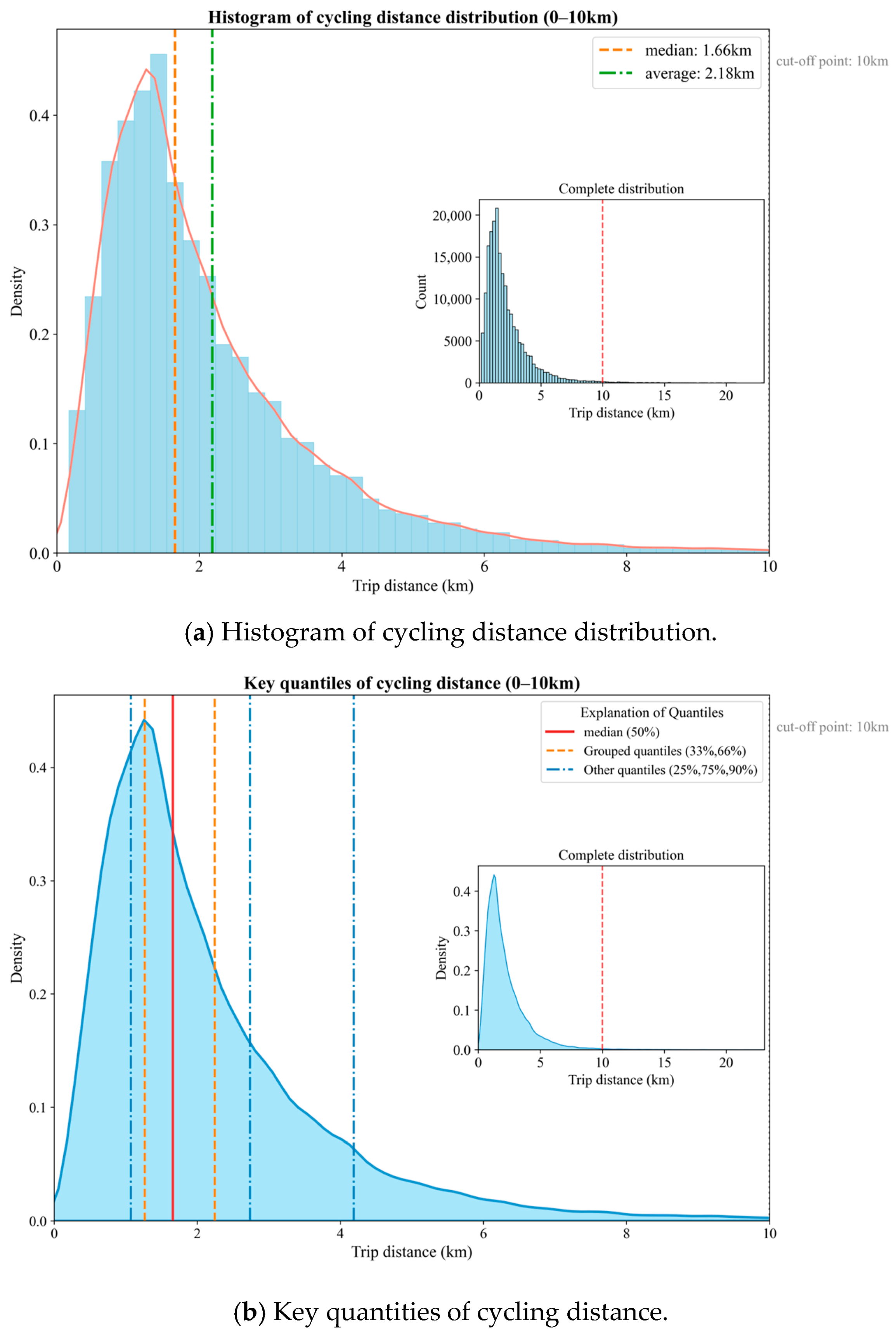
Based on the processed data, a distribution histogram of cycling distances was plotted. Since most cycling distances were below 10 km, the histogram was truncated at 10 km for clearer visualization. Figure 2a shows the frequency distribution of the riding distance of EBS in different intervals. The height of the blue bars represents the relative density of the number of rides within that distance interval. The red solid line covering the histogram is a theoretical distribution curve fitted based on actual data. The blue solid line in Figure 2b is the probability density curve of the riding distance, and the total area enclosed by the curve represents a probability of 1. As shown in Figure 2a,b, the median travel distance is 1.66 km. The 33rd and 25th percentiles are densely distributed to the left of 1.66 km, while the 75th and 90th percentiles are to the right. Since grouping by the median does not require a normal distribution of data, it is more representative of skewed distributions and is not affected by extremely large or small outliers. The median reflects the central tendency of the data. Using the median as a boundary to divide short and long-distance travel can more accurately represent the travel patterns of the majority of users. Dividing short and long-distance travel by the median also helps ensure the number of samples in each group, providing sufficient data support for the study, reducing the impact of randomness, and enhancing the power of statistical tests, making the differences between groups more significant. Additionally, research has shown that for the vast majority of travel purposes, when the travel distance exceeds 1 mile (approximately 1.6 km), the primary alternative modes shift from walking to bicycles, public transportation, or motorized vehicles [24]. Therefore, using 1.66 km as a threshold can effectively distinguish between short-distance travel primarily aimed at replacing walking and medium-to-long-distance travel targeting longer distances. This definition is well-founded in both statistical and behavioral science.
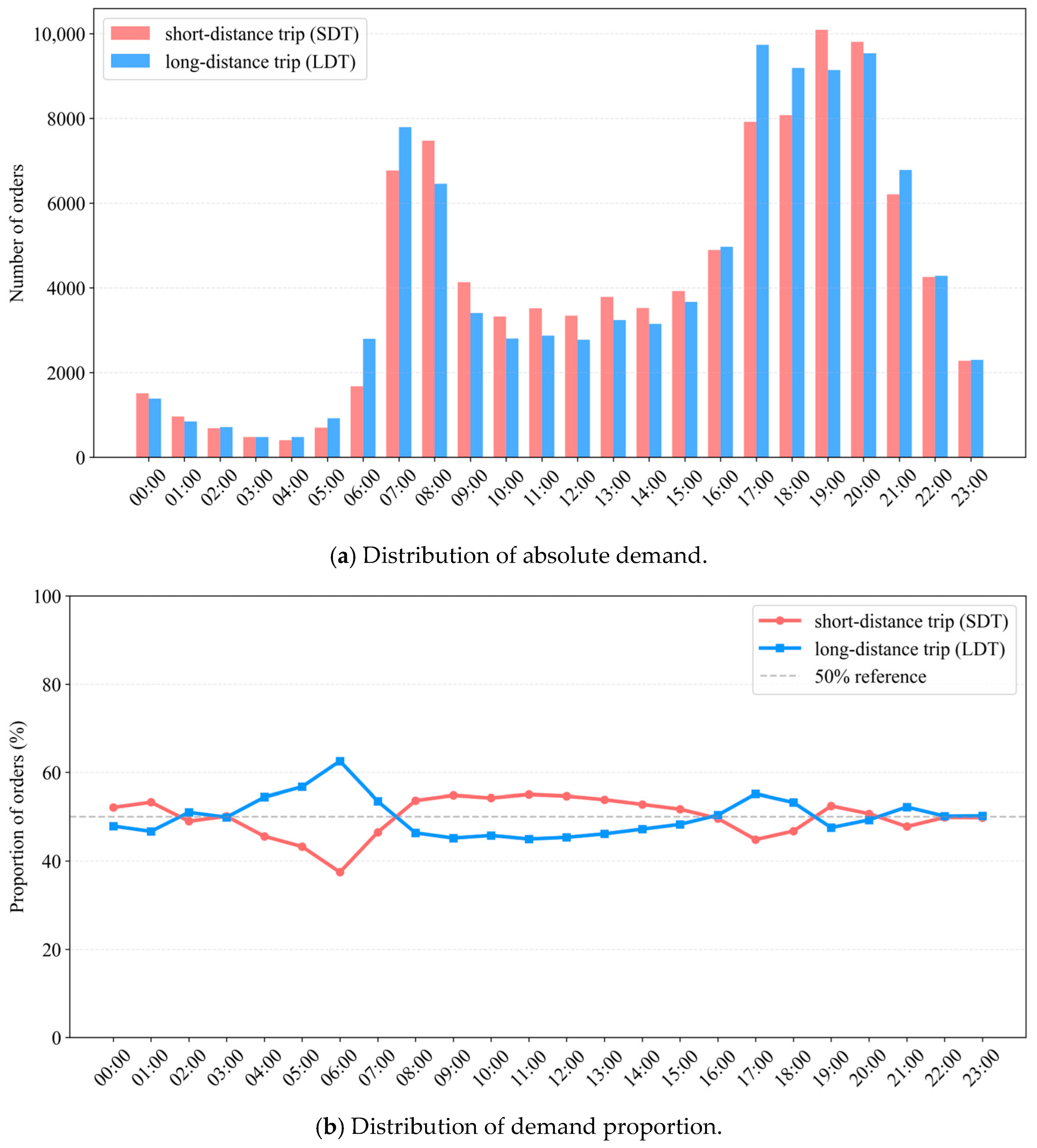
In terms of the temporal distribution of demand (Figure 3a,b), long-distance travel is highly concentrated during the morning and evening rush hours, demonstrating that it is mainly used to meet rigid commuting needs. The proportion of short-distance travel demand during the daytime is relatively stable, indicating that it is mainly used for short-distance connections and non-commuting purposes. The proportion remains high even at night, showing stronger adaptability throughout the day. Therefore, to analyze the differences in demand under different travel distances, this study uses 1.66 km as the median threshold to divide travel into two groups: long-distance and short-distance. This division ensures a balanced sample size while effectively distinguishing between the rigid demand mainly for commuting and the elastic demand mainly for short-distance connections, facilitating subsequent comparative analysis.

3.3. Variable Selection

In order to study the travel demand of EBS at different distance scales, the order volumes of short- and long-distance trips were taken as the dependent variables, which were obtained by counting the number of orders in each grid cell. At the same time, considering that various environmental factors affect the travel situation of EBS, 17 environmental variables were selected to explain short and long-distance travel, including 13 types of points of interest, 3 levels of road network density, and population density data. These variables have been verified in previous studies and have good explanatory power in studying the impact of the built environment on travel demand [6,7,20]. Existing studies have already examined various influencing variables on the use of EBS or BS, as shown in Table 1.
These variables were classified into three types: road network indicators, land use indicators, and public transportation indicators. Among them, the density of the road network was obtained by calculating the ratio of the road length to the grid area within each grid. Population density was obtained by calculating the ratio of the population number to the grid area within each grid. The indicators for POIs and public transportation were represented by the number of various types within the computing grid. Descriptive statistics of the variables used in the study are shown in Table 2.
(1)
Road network indicators
Roads, as the carriers of transportation, and road density determine the service coverage of EBS. The grade of roads also affects the safety of travel. Therefore, road network indicators influence the use of EBS.
(2)
Land use indicators
The use of EBS is closely related to the population base and socio-economic activities. Population density, to some extent, determines the amount of demand for EBS use. The number and types of POIs can also reflect the local commercial vitality, social life, and public services.
(3)
Public transport indicators
As a mode of transportation, EBS is directly affected by other public transportation facilities. Generally, in areas with more developed public transportation, the usage of EBS will correspondingly decrease. This study selects the number of bus stops to reflect the quality of public transportation and investigates its impact on the travel of EBS.
Table 2. Descriptive statistics of variables.
VariablesDescriptionAverageStdMinMax
Dependent Variables
LDTThe number of long-distance trips23.92114.3302063
SDTThe number of Short-distance trips23.92140.0103652
Road Network Indicators
Primary roadsTrunk road density (km/km2)0.501.46014.55
Secondary roadsSecondary road density (km/km2)0.361.11012.47
Tertiary roadsBranch density (km/km2)1.681.88013.95
Land Use Indicators
Population densityPopulation density (people/km2)822.85493.4806416
Catering servicesThe number of POIs of catering service facilities2.068.650152
CorporationsThe number of POIs of the company enterprise2.345.80071
Shopping servicesNumber of shopping service facility POIs4.9319.580420
Financial servicesNumber of POIs for financial services facilities0.120.72011
Culture and educational servicesThe number of POIs of educational and cultural service facilities0.341.27024
Living servicesNumber of POIs for life service facilities1.746.60079
Sports and leisure servicesNumber of POIs for leisure service facilities0.371.59042
Medical servicesNumber of POIs in medical facility0.411.73022
Government agencyThe number of POIs of government units0.602.02028
Accommodation servicesNumber of POIs for hotel accommodation facilities0.625.610148
Commercial residencesThe number of residential POIs in the community0.331.06012
Tourist attractionsThe number of POIs of attraction service facilities0.121.21047
Public Transport Indicators
Ground public transportNumber of bus stops0.300.6107

4. Methods

4.1. Theoretical Framework

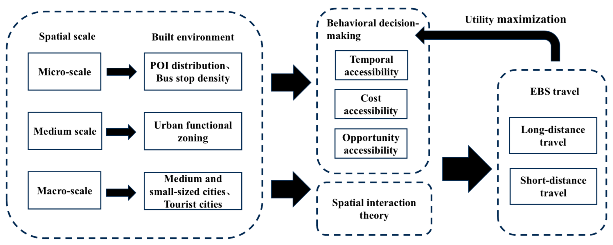
The demand for EBS travel is a rational choice made by travelers based on improved accessibility, under the constraints of urban spatial structure. The impact of different built environment elements (such as urban structure, land use, and POI distribution) exists at different spatial scales, including macro, medium, and micro levels. This theoretically explains the root of spatial heterogeneity. The differentiation of travel behavior between long and short distances is essentially the result of the differential effects of the built environment under different spatial heterogeneity conditions. Based on the above analysis, a theoretical framework has been constructed, as shown in Figure 4.
The framework starts with the built environment at multiple spatial scales. At the micro scale, it focuses on the impact of POI distribution and bus stop density. At the medium scale, it pays attention to urban functional zoning. At the macro scale, it is based on the characteristics of small and medium-sized tourist cities. The built environment features at all these scales together form the basis of influence. These environmental factors ultimately affect the travel behavior of EBS through the dual effects of behavioral decision-making and the spatial interaction theory, which is specifically manifested in the differences in choices between long-distance and short-distance travel. To accurately reveal the complex impact of the built environment at multiple spatial scales on the demand for EBS trips within the above theoretical framework, this study employs the MGWR model for empirical testing.

4.2. Spatial Autocorrelation

Spatial autocorrelation reflects the correlation between observations of the same variable at different spatial locations. The fundamental concept of spatial autocorrelation is that data values at spatially adjacent or close locations may exhibit some degree of dependence or similarity, which tends to diminish or vanish as the distance increases. To assess the overall spatial association patterns of the influencing variables within Tongxiang City, and to examine whether the spatial data show a tendency towards clustering or dispersion, as well as the strength and significance of such trends, it is necessary to conduct a comprehensive measurement of the spatial data across the entire study area. Therefore, global spatial autocorrelation is employed.
The range of Moran’s I statistic is [−1, +1], which can determine whether the variable has spatial autocorrelation and the degree of spatial autocorrelation [27]. When the Moran’s I statistic is positive, it indicates the spatial clustering of the variable; when it is negative, it indicates the spatial dispersion of the variable; and when close to zero, it indicates a random spatial distribution of the variable. The mathematical expression of Moran’s I is as follows:
I = n i = 1 n j = 1 n w i j x i x x j x i = 1 n x i x 2 i = 1 n j = 1 n w i j
where x i represents the observation of the i-th region, which is the quantified influencing factor in this study. n is the total number of regions, in this study is the number of influencing factors, and w i j is the spatial weight matrix constructed based on the observations.

4.3. Regression Model

To evaluate the factors influencing short- and long-distance travel, this study established three regression models: the Ordinary Least Squares (OLS) model, the Geographically Weighted Regression (GWR) model, and the Multiscale Geographically Weighted Regression (MGWR) model. The adjusted R2 and AICc values of the three models were compared to select the most suitable model for in-depth exploration in this study. OLS is a fundamental regression analysis method in statistics. Its core idea is to minimize the sum of squared residuals, thereby fitting a straight line that is the closest to the target relationship and obtaining the regression coefficients. In this study, it is used to calculate the regression coefficients of the short- and long-distance travel situations and influencing factors. In the OLS model, it is assumed that the relationship between the dependent variable and the independent variable is at a fixed ratio. However, if the actual relationship is a more complex nonlinear relationship, the fitting degree will be poor. Its mathematical expression is as follows:
Y i = β i 0 + n = 1 m β i n X i n + ε i
where i represents the i-th grid cell; Y i represents the dependent variable of the i-th grid cell; X i n is the n-th independent variable; β i 0 denotes the intercept term; β i n denotes the regression coefficient of the n-th influencing factor; m represents the number of grid cells; ε i denotes the error term of the i-th grid.
Before establishing the regression models, it is necessary to conduct multicollinearity tests on the variables and remove those with extremely strong correlations with other explanatory variables to avoid issues such as unstable model coefficient estimates, invalid t-tests, and reduced prediction accuracy caused by multicollinearity [28]. To quantify the degree of collinearity between variables and capture complex collinearity relationships, this study uses the Variance Inflation Factor (VIF) to address multicollinearity among the factors influencing short- and long-distance travel. This indicator is generally considered to indicate severe multicollinearity when it exceeds 5 [29]. In this study, variables with VIF values greater than 5 were first removed, followed by running the OLS model to exclude variables with poor significance levels [30]. The formula for calculating VIF is as follows:
V I F = 1 1 R i 2
where R i 2 is the negative correlation coefficient of the regression analysis of the independent variable x i against the other independent variables. In this study, it is the negative correlation coefficient obtained from the regression analysis of a certain indicator against the other independent variables.
Compared to the traditional OLS model, the GWR model allows parameters to change locally, enabling the relationships between variables to vary with geographical location. It can reflect overlooked local characteristics and also permits spatial non-stationarity in spatial assumptions. It can effectively interpret the spatial variation relationship patterns and address the issue of spatial heterogeneity. Its mathematical expression is as follows [31]:
Y i = β i 0 ( u i , v i ) + k β i k ( u i , v i ) X i k + ε i
where i denotes the i-th grid cell, Y i denotes the dependent variable for the i-th grid cell, u i , v i are the geographic coordinates of the i-th grid cell, X i k is the k-th explanatory variable of the i-th grid cell, β i 0 u i , v i represents the intercept for the i-th grid cell, β i k u i , v i represents the regression coefficient of the k-th explanatory variable for the i-th grid cell, and ε i represents the error term for the i-th grid.
Although the GWR model has improved the issue of constant global parameters, all independent variables still use the same bandwidth. To address this drawback, this study attempts to make improvements on the GWR model and establish the MWGR model to achieve more accurate experimental results. The MGWR assumes that the spatial scales of all local coefficients can be different and uses the optimal bandwidth for each explanatory variable for regression, significantly reducing the risk of overfitting and clearly separating multi-scale effects. Its mathematical expression is as follows [32]:
Y i = β b w 0 ( u i , v i ) + k β b w k ( u i , v i ) X i k + ε i
where β b w 0 u i , v i represents the regression constant for the i-th grid cell under the b w 0 bandwidth condition, β b k w u i , v i represents the regression coefficient for the k-th explanatory variable in the i-th grid cell under the b w k bandwidth condition, and ε i represents the error term for the i-th grid.

5. Model Results

5.1. Multicollinearity Tests and Spatial Autocorrelation Tests

To address the issue of multicollinearity among the explanatory variables, a Pearson correlation coefficient test was first conducted on 16 independent variables. It was found that the correlation coefficients between the explanatory variable “Catering Services” and “Shopping Services”, “Living Services”, and “Medical Services” were 0.71, 0.85, and 0.72, respectively; between “Living Services” and “Shopping Services”, “Medical Services”, and “Sports and Leisure Services”, the correlation coefficients were 0.71, 0.78, and 0.62, respectively. At the same time, the VIF values of each explanatory variable are obtained by using the least squares regression. Secondly, a global autocorrelation test was conducted. The results of the Moran’s I test are shown in Table 3. Through stepwise regression, seven independent variables were selected, with all their VIF values being less than 5, indicating that there is no multicollinearity among these explanatory variables [26]. The P-values of each variable are all less than 0.05, and the Z-values are all positive, indicating that these variables have significant spatial correlation and agglomeration. The results of the multicollinearity test and spatial autocorrelation test for seven independent variables are shown in Table 3.

5.2. Comparison of Model Results

To demonstrate the superior performance of the MGWR model, GWR and MGWR models were established for 17 explanatory variables with LDT and SDT as dependent variables, respectively, and the model fit was assessed through four diagnostic indicators. The relevant results are shown in Table 4. Among them, the smaller the AICc value, and the higher the R2 and R2Adj values, the better the model’s fitting performance, and the more capable it is of describing the spatial heterogeneity of the EBS travel demand. In the model for long-distance demand, the R2 value of the MGWR model increased by 0.24 and 0.153, respectively, compared to the GWR and OLS models; the adjusted R2 value increased by 0.195 and 0.137, respectively, compared to the GWR and OSL models; the AICc value decreased by 81.723 and 4874.988, respectively, compared to the GWR and OSL models. From the perspective of bandwidth, the global OLS model has a bandwidth of 424, which is the total number of samples; the local GWR model assumes that the spatial scale of the effect of all variables is the same, which is 322. The MGWR model assumes that different variables have different spatial scales of influence, with its bandwidth range being [68, 423]. Meanwhile, the sum of squared residuals for the MGWR model with LDT as the dependent variable is 123.892, while that for the GWR model is 225.478; the sum of squared residuals for the MGWR model with SDT as the dependent variable is 169.634, while that for the GWR model is 275.874.
Traditional ordinary least squares (OLS) regression assumes that the relationships between variables are constant throughout the study area. It produces a set of globally averaged parameter estimates, which means that the impact of influencing factors on land value is identical in both the city center and the suburbs. This clearly does not align with the heterogeneous reality of urban spaces, as different urban areas are at different stages of development, have varying functional orientations, and possess distinct socioeconomic characteristics. The GWR model employs a single optimal bandwidth for all variables. This is equivalent to assuming that all influencing factors, such as banks, schools, and roads, operate at the same spatial scale. The use of a single optimal bandwidth may not reflect the spatial scales of some specific variables, leading to inaccurate fitting results. The core innovation of MGWR lies in its independent estimation of an optimal bandwidth for each explanatory variable. This allows different processes to operate at different spatial scales.
Based on the above data, the MGWR model performs better in reflecting the spatial heterogeneity and non-stationarity of the explanatory variables.

5.3. Analysis of Model Results

The MGWR model was reconstructed for the independent variables that had a significant impact and passed the multicollinearity test. The results showed that the coefficient of determination for long-distance travel was 0.594, and for short-distance travel, it was 0.501. Both fitting effects were better than those of the GWR model. When analyzing highly discrete and stochastic issues such as individual travel choices, the R2 value of the model is usually lower than that of the models in many natural science fields. Similar R2 ranges have also been reported in studies on BS or EBS. As Chen et al. [6] reported in their study on the spatiotemporal travel patterns and influencing factors of BS and EBS systems, the range of the coefficient of determination was 0.607–0.671. In the study by Li et al. [33] on the impact of the built environment on dockless BS oriented by the subway, the reported range of the coefficient of determination was 0.498–0.559. The results of the MGWR model are presented in Table 5. Among them, the bandwidth values of the regression parameters for each explanatory variable are different, reflecting that the impact of the built environment indicators on the demand for short- and long-distance EBS travel has spatial non-stationarity and spatial heterogeneity in different areas.
The value of bandwidth represents the spatial scale of the effect of the explanatory variable on the demand for EBS trips. The smaller the value, the greater the spatial heterogeneity of the variable’s effect range; conversely, the larger the value, the smaller the heterogeneity. In the long-distance model, the spatial scale of shopping services and primary road density is smaller, indicating that these variables have greater spatial heterogeneity in the demand for long-distance EBS trips. The influence scales of cultural and educational services, commercial residences, sports and leisure services, accommodation services, and bus stations are relatively large, reflecting that these variables have less spatial heterogeneity in the demand for long-distance EBS trips. In the short-distance model, the spatial scale of shopping services, sports and leisure services, and primary road density is smaller, indicating greater spatial heterogeneity of these variables in the demand for short-distance trips. Conversely, the spatial scale of cultural and educational services, commercial residences, accommodation services, and bus stations is larger, showing that these variables have less spatial heterogeneity in the demand for short-distance trips.
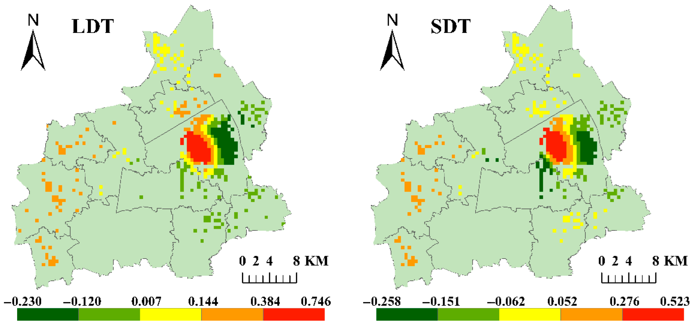
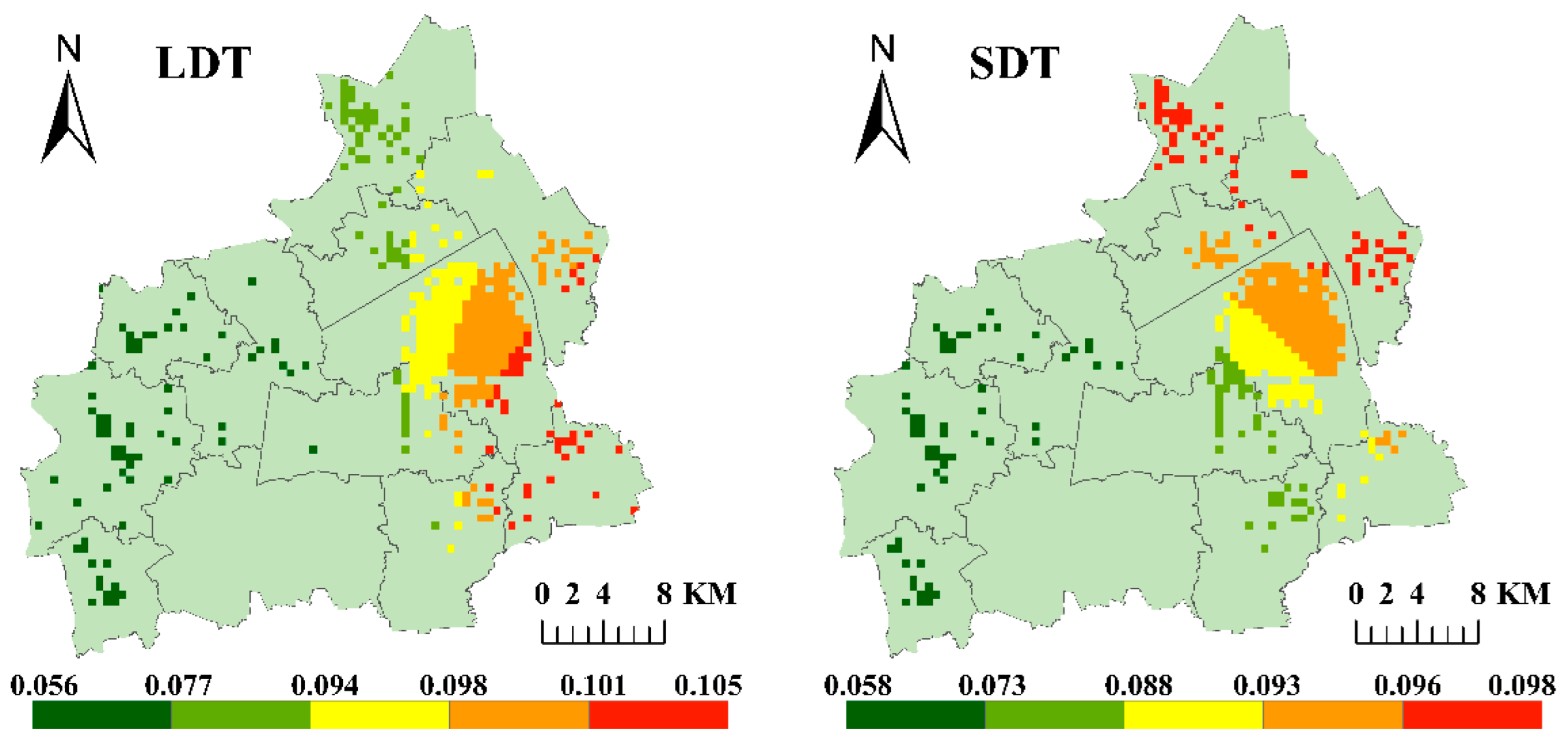
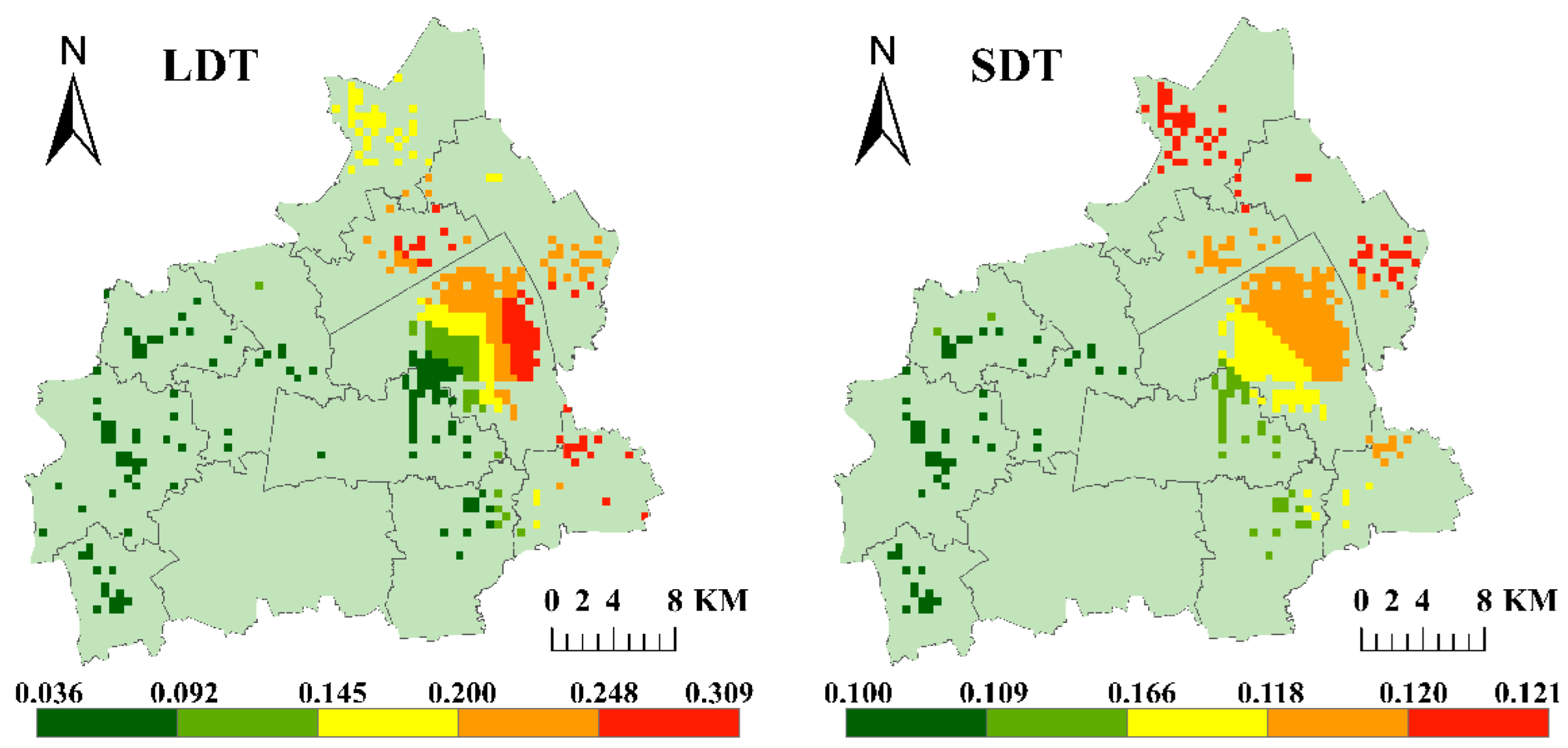
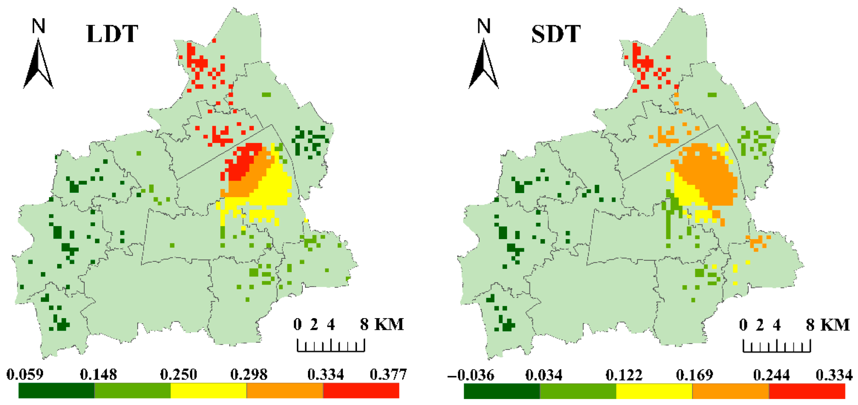
To visually illustrate the relationship between the relevant explanatory variables and the demand for EBS trips, seven explanatory variables were selected: shopping services, commercial residences, sports and leisure services, accommodation services, bus stations, and primary road density. These variables were selected to analyze the spatial heterogeneity of the MGWR model regression coefficients at different distance scales. The estimation results of the model were visualized using ArcGIS software. The spatial distribution of the coefficients for the relevant explanatory variables is shown in Figure 5, Figure 6, Figure 7, Figure 8, Figure 9 and Figure 10.

6. Discussion

Regarding the road indicators, Figure 5 shows the spatial distribution of the regression coefficients for arterial road density. For long-distance and short-distance EBS travel, the regression coefficients exhibit a clear gradient change from west to east in the main urban area. This spatial pattern suggests that the impact of arterial road density on EBS demand is not static but deeply dependent on the local traffic environment and development context.
Specifically, in the southeast part of the main urban area, a higher density of primary roads shows a suppressive effect on the EBS demand. This is inferred to mainly stem from the competitive relationship between different modes of transportation. This area is typically a well-developed urban core with a complete road network, higher private car ownership rates among residents, and dense coverage of regular public transport services. Therefore, for medium-to-long-distance travel, residents are more likely to choose private cars or public transportation, thereby reducing the relative attractiveness of EBS. In sharp contrast, in areas with relatively weak transportation infrastructure, such as the outskirts of Tongxiang City, the primary road density has a positive or neutral impact on EBS demand. This indicates that in such environments, the relationship between EBS and public transportation is more complementary than competitive. Due to the sparse bus routes and fewer schedules in the peripheral areas, there is a significant “first mile” and “last mile” problem. EBS happens to fill this service gap.
Figure 5. The distribution of regression coefficients for primary roads density.
Sustainability 17 10437 g005
The distribution of the regression coefficients for bus stops is shown in Figure 6. The overall positive impact of bus stops on the EBS travel demand in the main urban area indicates a certain degree of complementarity between the two. This complementarity is primarily reflected in the function of connecting different modes of transportation. The dense bus network in the main urban area serves as the backbone for residents’ long-distance travel, while EBS acts as an ideal “last mile” solution, effectively extending the service radius of bus stops and enhancing the accessibility of the entire public transportation system. This is especially evident in the Wuzhen Scenic Area in the northern part of Tongxiang City. After arriving by bus or taxi, tourists generate a large number of short-distance travel demands within and around the scenic area, which are conveniently met by EBS. This highlights its value as an activity-end extension tool in tourism contexts.
In contrast, in the city center where the long-distance travel demand is more pronounced, it is inferred that there is a competitive relationship between EBS and buses during long-distance commuting. When the travel distance falls within the advantageous range of EBS and the urban infrastructure in the city center can support its efficient and safe operation, EBS is no longer just a connecting tool but becomes a direct competitor to bus services. According to the theory of individual utility maximization in mode choice, travelers weigh time costs, economic costs, flexibility, and comfort when selecting a mode of transportation. In the main urban area, the flexible and fast service of EBS avoids the need for transfers, waiting, and walking, thereby leading to a substitution effect on bus travel. This finding is consistent with previous studies [25], which found that the operation of EBS had a significant negative impact on bus passenger volumes. Therefore, the competitive and complementary relationship between EBS and buses is not static and may be influenced by the travel distance, urban layout, and transportation structure. Given the limited travel options in small and medium-sized cities, this phenomenon may be more pronounced.
Figure 6. The distribution of regression coefficients for bus stops.
Sustainability 17 10437 g006
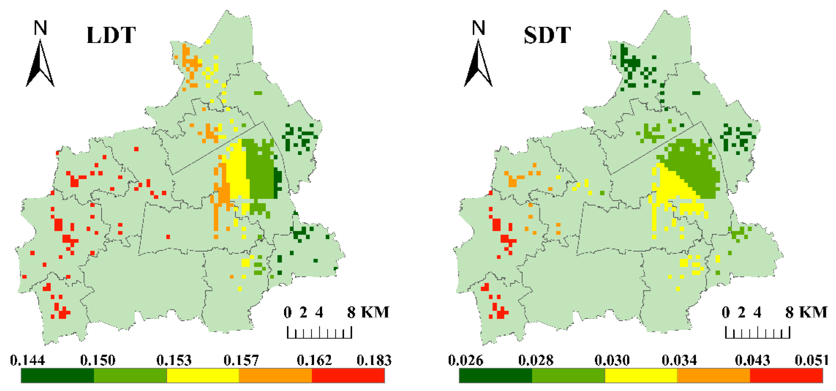
The distribution of regression coefficients for leisure and shopping services is shown in Figure 7 and Figure 8. The strong attractiveness of leisure services in the eastern part of the main urban area to long-distance travel is the result of the combined effects of the city’s monocentric structure and mixed land use development. Centered around the Phoenix Lake Scenic Area, this region has a highly mixed pattern of commercial, industrial, and residential functions. The concentration of large urban commercial complexes (such as Wuyue Plaza) and regional leisure facilities (such as theaters and sports stadiums) creates a powerful destination appeal, sufficient to attract residents to make special long-distance trips. Previous studies have also found [3] that commercial districts with a concentration of entertainment activities greatly promote the use of EBS. More importantly, the functional mix enables residents to complete multiple purposes such as “shopping, dining, and leisure entertainment” in one trip. This multipurpose travel chain characteristic naturally fits the flexible, door-to-door advantages of EBS, thereby significantly increasing the demand for long-distance travel.
Figure 7. The distribution of regression coefficients for sports and leisure services.
Sustainability 17 10437 g007
In contrast, the western part of the main urban area lacks such large gravitational centers, and leisure services are characterized by dispersion and community orientation. This layout mainly meets residents’ daily and nearby needs, generating mostly single-purpose short-distance trips, which is essentially different from the compound and purpose-driven long-distance travel generated in the east. The positive impact of shopping services in the northwest shown in Figure 8 corroborates this view. Due to the lack of large commercial complexes locally, residents have to choose long-distance cycling or other transportation modes to go to the central and eastern business districts. This indirectly proves that the spatially uneven distribution of urban service facilities is a key driver in shaping EBS travel patterns.
Figure 8. The distribution of regression coefficients for shopping service.
Sustainability 17 10437 g008
The distribution of regression coefficients for commercial residences areas is shown in Figure 9. In the southwest part of the central urban area, where commercial residential areas are concentrated, there is a clear positive correlation with long-distance EBS travel. This pattern profoundly reflects the regional differences in job–housing spatial relationships and transportation service levels in Tongxiang City. Due to the distinct separation of industrial and residential land use in the southwest part of the central urban area, middle-aged and young, middle-income commuters living in this area, with their high value of time and pursuit of efficiency, may be willing to choose EBS as the optimal solution to avoid congestion and achieve efficient point-to-point commuting. On the other hand, in towns farther from the central urban area, the promotion of travel demand by commercial residential areas is inferred to stem from a different mechanism: the lack of public transportation services. These areas suffer from an insufficient coverage of bus stations, and even if residents want to use public transportation, they face the challenge of solving the first or last mile of their journey. Here, EBS plays a key role in the multimodal transportation chain, effectively expanding the activity range of residents and enhancing the overall travel accessibility. This finding echoes our discussion on bus stops, jointly illustrating the indispensable complementary role of EBS in areas with weak public transportation.
Figure 9. The distribution of regression coefficients for commercial residences.
Sustainability 17 10437 g009
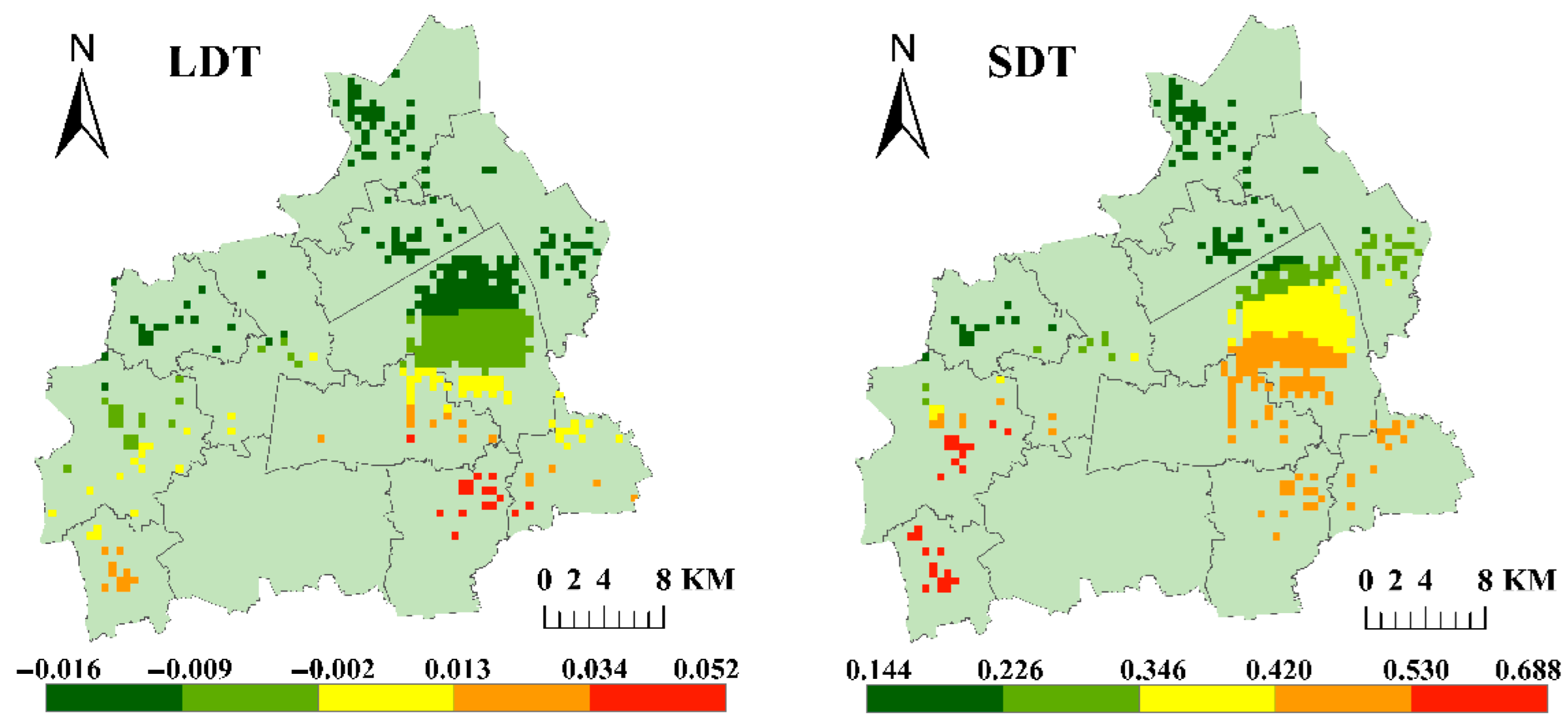
The distribution of regression coefficients for accommodation services is shown in Figure 10. Accommodation services have a clear suppressive impact on long-distance EBS travel in the main urban area but show a significant positive impact on short-distance travel, especially in the southern part of the main urban area where there is a higher density of accommodation services. As a well-known tourist city, Tongxiang attracts a large number of visitors. As temporary residents, tourists’ core goal is to efficiently visit multiple nearby attractions and facilities within a limited time. The southern part of the main urban area, with its dense accommodation facilities, typically aggregates tourist sites, dining, and commercial outlets. This spatial pattern naturally generates high-frequency, multipurpose short-distance travel chains. The flexible, easy-to-use, and economical nature of EBS perfectly meets tourists’ needs to build an efficient “activity chain”, making it an ideal tool for connecting accommodation sites with surrounding activity nodes. This finding is similar to previous research [15], which found that in tourist cities, 85% of travel orders are made by tourists, and most users use EBS to go to leisure and entertainment venues. In contrast, the suppressive impact of accommodation services on long-distance travel reflects the competition among different modes of transportation based on travel utility. When the travel destination is far away (such as to suburban scenic areas or transportation hubs), the criteria for travel decision-making shift from convenience to the overall experience and efficiency. In this context, taxis or ride-hailing services, which offer point-to-point services and higher comfort levels, have a significantly higher overall utility than EBS. The latter’s disadvantages in terms of physical exertion, weather conditions, and safety become more pronounced in long-distance travel. This indicates that in the tourism transportation system, EBS is primarily positioned for short-to-medium distance microcirculation rather than competing with motorized travel modes in long-distance scenarios.
Figure 10. The distribution of regression coefficients for accommodation services.
Sustainability 17 10437 g010

7. Policy Recommendation

Based on the research findings and the actual situation in Tongxiang City, this paper proposes several targeted and feasible policy recommendations from the perspectives of government departments and EBS companies to optimize the user experience of EBS. These recommendations can also serve as a reference for the optimized development of EBS in other small and medium-sized cities.
(1)
Implementation of precise planning and management
In large residential areas and peripheral regions with weak public transportation services, the demand stems from commuting connections and basic travel needs. Policies should encourage operators to optimize vehicle distribution to ensure service coverage. Meanwhile, the government can incorporate EBS accessibility into the evaluation system for public transportation services to compensate for the shortcomings of fixed bus routes and ensure travel equity for residents in different areas. In the urban core and commercial centers, it is recommended to designate electronic fence parking zones. Through data-sharing platforms with operators, real-time alerts and intelligent scheduling for excessive deployment and disorderly parking can be achieved. The core objective is to ensure the smooth flow of sidewalks and maintain urban order, rather than blindly expanding the scale.
(2)
Coordinated optimization of the transportation system
On long-distance routes where buses and EBS form excessively strong competition, the transportation department should reassess the efficiency of bus services. Consider optimizing bus routes, increasing the frequency of departures, and launching express bus lines to enhance core competitiveness. Position EBS as an effective supplement to bus services during specific times (such as at night) and in specific areas, rather than simply prohibiting them. This approach can lead to differentiated development and a coordinated, efficient green transportation system.
(3)
Improve the construction of road infrastructure
In areas where there is a positive correlation between primary road density and cycling demand, future road renewal and transformation should prioritize the planning and construction of a continuous and safe non-motorized vehicle lane network. This is not only a response to the current demand, but also an active effort to guide residents to form green travel habits by enhancing safety and comfort.

8. Conclusions

To analyze the spatiotemporal heterogeneity of influencing factors on the EBS travel demand at different travel distances in small and medium-sized cities, this paper constructs a multi-scale geographical weighted regression model based on the EBS order data in Tongxiang City to analyze the main influencing factors and their spatial heterogeneity of the long-distance and short-distance EBS travel demand. The conclusions are as follows:
(1)
Compared to the OLS and GWR models, the MGWR model has significant advantages in revealing the spatial heterogeneity of the impact of each explanatory variable on the EBS travel demand for both long and short distances.
(2)
The demand for short-distance travel is prominent around scenic spots, accommodation sites, and bus stops. EBS serves the function of shuttling tourists and the “last mile” connectivity, complementing buses. However, in the main urban area with a well-developed road network, EBS competes with and substitutes buses in long-distance travel.
(3)
In long-distance travel, leisure services and shopping services have significant positive impacts on the EBS use in the eastern and northwestern parts of the main urban area, respectively. The eastern part of the main urban area has a denser distribution of large commercial complexes, attracting long-distance travelers. This indicates that residents are willing to travel across regions to engage in multi-purpose leisure activities, and EBS is one of the main modes of transportation for travelers heading to large leisure venues or commercial complexes.
(4)
The impact of the built environment on EBS use has significant context dependency. Commercial residential areas in the western job–residential separation area promote long-distance commuting, while leisure services in the eastern commercial district attract long-distance consumption travel, reflecting the structural influence of the urban functional layout on travel behavior.
This study has some limitations that provide directions for future research. First, since the data did not record user attributes, future research will rely on questionnaire surveys to explore the impact of population characteristics on EBS travel distance. Second, this study focused on spatial heterogeneity without considering the temporal dimension (such as weekdays/weekends). Subsequent research could employ the GTWR model to reveal the spatiotemporal evolution patterns. Third, the data were only sourced from July, which is the peak tourist season. Future research needs to incorporate data from multiple seasons to disentangle and compare the travel demand differences between residents and tourists, thereby gaining a more comprehensive understanding of usage patterns.

Author Contributions

Data curation, X.W.; Resources, X.L. and M.D.; Software, X.W.; Supervision, F.L. and J.-Y.K.; Writing—original draft preparation, X.W., Z.P., X.L. and K.L.; Writing—review and editing, X.W., Z.P., D.L. and M.D. All authors have read and agreed to the published version of the manuscript.

Funding

This research was funded by the Humanities and Social Science Fund of the Ministry of Education of China (No. 23YJCZH042), China Postdoctoral Science Foundation (No. 2025M771623), the National Natural Science Foundation of China (No. 52302392), the Natural Science Research of Jiangsu Higher Education Institutions of China (No. 23KJB580011), the General Project for Philosohy and Social Science Research in Jiangsu Higher Education Institutions of China (2024SJYB0135).

Institutional Review Board Statement

Not applicable.

Informed Consent Statement

Not applicable.

Data Availability Statement

Data will be made available on request.

Acknowledgments

The authors thank Tongxiang Public Bicycle Service Co., LTD for providing the data.

Conflicts of Interest

The authors declare no conflicts of interest.

References

  1. Zhou, Y.; Yu, Y.; Wang, Y.; He, B.; Yang, L. Mode substitution and carbon emission impacts of electric bike sharing systems. Sustain. Cities Soc. 2023, 89, 104312. [Google Scholar] [CrossRef]
  2. Wang, Q.; He, B.; Yan, Z. Effect of Built Environment on Activity-Travel Behavior: A Comparative Study between Kunming and Qujing. In CICTP 2019, Proceedings of the 19th COTA International Conference of Transportation Professionals, Nanjing, China, 6–8 July 2019; American Society of Civil Engineers: New York, NY, USA, 2019; pp. 6044–6056. [Google Scholar]
  3. Li, Q.; Qin, Y.; Xu, W. Is there a link between city characteristics and shared e-bike utilisation? Evidence from China. Sustain. Cities Soc. 2025, 120, 106008. [Google Scholar] [CrossRef]
  4. Li, Y.; Dai, Z.; Zhu, L.; Liu, X. Analysis of spatial and temporal characteristics of citizens’ mobility based on e-bike GPS trajectory data in Tengzhou City, China. Sustainability 2019, 11, 5003. [Google Scholar] [CrossRef]
  5. Yang, Y.; Li, T.; Zhang, T.; Yang, W. Understanding the utilization characteristics of bicycle-sharing systems in underdeveloped cities: A case study in Xuchang City, China. Transp. Res. Rec. 2017, 2634, 78–85. [Google Scholar] [CrossRef]
  6. Chen, Y.; Xu, S.; Du, M.; Ma, H.; Wang, S.; Li, F. Comparing the Spatiotemporal Travel Patterns and Influencing Factors of Bike Sharing and E-Bike Sharing Systems. Int. Arch. Photogramm. Remote Sens. Spat. Inf. Sci. 2023, 48, 339–345. [Google Scholar] [CrossRef]
  7. Li, A.; Zhao, P.; Huang, Y.; Gao, K.; Axhausen, K.W. An empirical analysis of dockless bike-sharing utilization and its explanatory factors: Case study from Shanghai, China. J. Transp. Geogr. 2020, 88, 102828. [Google Scholar] [CrossRef]
  8. Tang, T.; Guo, Y.; Zhou, X.; Labi, S.; Zhu, S. Understanding electric bike riders’ intention to violate traffic rules and accident proneness in China. Travel Behav. Soc. 2021, 23, 25–38. [Google Scholar] [CrossRef]
  9. Li, J.; Shen, J.; Jia, B. Exploring intention to use shared electric bicycles by the extended theory of planned behavior. Sustainability 2021, 13, 4137. [Google Scholar] [CrossRef]
  10. Li, W.; Yang, Y.; Cheng, L.; Meng, X.; Zhang, F.; Ji, Y. Understanding adoption intent and behavioral response to shared electric bicycles: A survey in Ningbo, China. Transp. Res. Rec. 2023, 2677, 1311–1326. [Google Scholar] [CrossRef]
  11. Campbell, A.A.; Cherry, C.R.; Ryerson, M.S.; Yang, X. Factors influencing the choice of shared bicycles and shared electric bikes in Beijing. Transp. Res. Part C Emerg. Technol. 2016, 67, 399–414. [Google Scholar] [CrossRef]
  12. Chen, J.; Zhang, Y.; Zhang, R.; Cheng, X.; Yan, F. Analyzing users’ attitudes and behavior of free-floating bike sharing: An investigating of Nanjing. Transp. Res. Procedia 2019, 39, 634–645. [Google Scholar] [CrossRef]
  13. Li, X.; Zhang, Y.; Sun, L.; Liu, Q. Free-floating bike sharing in jiangsu: Users’ behaviors and influencing factors. Energies 2018, 11, 1664. [Google Scholar] [CrossRef]
  14. Ning, J.; Chen, J.; Chen, X.; Yu, X. Traveler preference analysis between dockless bike-sharing and electric bike-sharing in last-mile metro context: Insights from Nanjing’s urban and suburban areas. Travel Behav. Soc. 2025, 40, 100999. [Google Scholar] [CrossRef]
  15. He, Y.; Song, Z.; Liu, Z.; Sze, N. Factors influencing electric bike share ridership: Analysis of Park City, Utah. Transp. Res. Rec. 2019, 2673, 12–22. [Google Scholar] [CrossRef]
  16. Guidon, S.; Becker, H.; Dediu, H.; Axhausen, K.W. Electric bicycle-sharing: A new competitor in the urban transportation market? An empirical analysis of transaction data. Transp. Res. Rec. 2019, 2673, 15–26. [Google Scholar] [CrossRef]
  17. Ma, X.; Ji, Y.; Yuan, Y.; Van Oort, N.; Jin, Y.; Hoogendoorn, S. A comparison in travel patterns and determinants of user demand between docked and dockless bike-sharing systems using multi-sourced data. Transp. Res. Part A Policy Pract. 2020, 139, 148–173. [Google Scholar] [CrossRef]
  18. Lang, H.; Zhang, S.; Fang, K.; Xing, Y.; Xue, Q. What Is the Impact of a Dockless Bike-Sharing System on Urban Public Transit Ridership: A View from Travel Distances. Sustainability 2023, 15, 10753. [Google Scholar] [CrossRef]
  19. Shi, Z.; Wang, J.; Liu, K.; Liu, Y.; He, M. Exploring the usage efficiency of electric bike-sharing from a spatial–temporal perspective. Transp. Res. Part D Transp. Environ. 2024, 129, 104139. [Google Scholar] [CrossRef]
  20. Gou, C.; Feng, C.; Tan, S.; Guo, M.; Li, R.; Zhao, F. Evaluating the impact of built environment on shared electric bicycle connectivity in kunming’s public transport system. Sci. Rep. 2025, 15, 5156. [Google Scholar] [CrossRef] [PubMed]
  21. Zhu, Y.; Yang, Z.; Feng, X.; Cheng, C.; Guo, Y.; Li, Q.; Wu, T.; Li, X.; Witlox, F. Comparing built environment effects on bike-sharing and electric bike-sharing usage: A spatiotemporal machine learning approach. Transp. Res. Part A Policy Pract. 2025, 200, 104642. [Google Scholar] [CrossRef]
  22. Tang, J.H.C.G.; Huang, Y.; Zhu, Y.; Yang, X.; Zhuge, C. The association between travel demand of docked bike-sharing and the built environment: Evidence from seven US cities. Sustain. Cities Soc. 2024, 106, 105325. [Google Scholar] [CrossRef]
  23. Wu, C.; Kim, I.; Chung, H. The effects of built environment spatial variation on bike-sharing usage: A case study of Suzhou, China. Cities 2021, 110, 103063. [Google Scholar] [CrossRef]
  24. Fukushige, T.; Fitch, D.T.; Handy, S. Factors influencing dock-less E-bike-share mode substitution: Evidence from Sacramento, California. Transp. Res. Part D Transp. Environ. 2021, 99, 102990. [Google Scholar] [CrossRef]
  25. Chen, J.; Liu, X.; Chen, X.; Wang, Y. Influence of e-bikeshare on transit ridership in a medium-sized Chinese city. Transp. Res. Part D Transp. Environ. 2025, 139, 104564. [Google Scholar] [CrossRef]
  26. Waldner, F.; Balke, G.; Rech, F.; Lellep, M. Data-driven insights into (E-) bike-sharing: Mining a large-scale dataset on usage and urban characteristics: Descriptive analysis and performance modeling. Transportation 2025, 1–41. [Google Scholar] [CrossRef]
  27. Gedamu, W.T.; Plank-Wiedenbeck, U.; Wodajo, B.T. A spatial autocorrelation analysis of road traffic crash by severity using Moran’s I spatial statistics: A comparative study of Addis Ababa and Berlin cities. Accid. Anal. Prev. 2024, 200, 107535. [Google Scholar] [CrossRef]
  28. Vandenbulcke, G.; Dujardin, C.; Thomas, I.; de Geus, B.; Degraeuwe, B.; Meeusen, R.; Panis, L.I. Cycle commuting in Belgium: Spatial determinants and ‘re-cycling’strategies. Transp. Res. Part A Policy Pract. 2011, 45, 118–137. [Google Scholar] [CrossRef]
  29. Pan, Y.; Chen, S.; Niu, S.; Ma, Y.; Tang, K. Investigating the impacts of built environment on traffic states incorporating spatial heterogeneity. J. Transp. Geogr. 2020, 83, 102663. [Google Scholar] [CrossRef]
  30. Moran, P.A. Notes on continuous stochastic phenomena. Biometrika 1950, 37, 17–23. [Google Scholar] [CrossRef]
  31. Brunsdon, C.; Fotheringham, A.S.; Charlton, M.E. Geographically weighted regression: A method for exploring spatial nonstationarity. Geogr. Anal. 1996, 28, 281–298. [Google Scholar] [CrossRef]
  32. Fotheringham, A.S.; Yang, W.; Kang, W. Multiscale geographically weighted regression (MGWR). Ann. Am. Assoc. Geogr. 2017, 107, 1247–1265. [Google Scholar] [CrossRef]
  33. Li, Z.; Shang, Y.; Zhao, G.; Yang, M. Exploring the multiscale relationship between the built environment and the metro-oriented dockless bike-sharing usage. Int. J. Environ. Res. Public Health 2022, 19, 2323. [Google Scholar] [CrossRef] [PubMed]
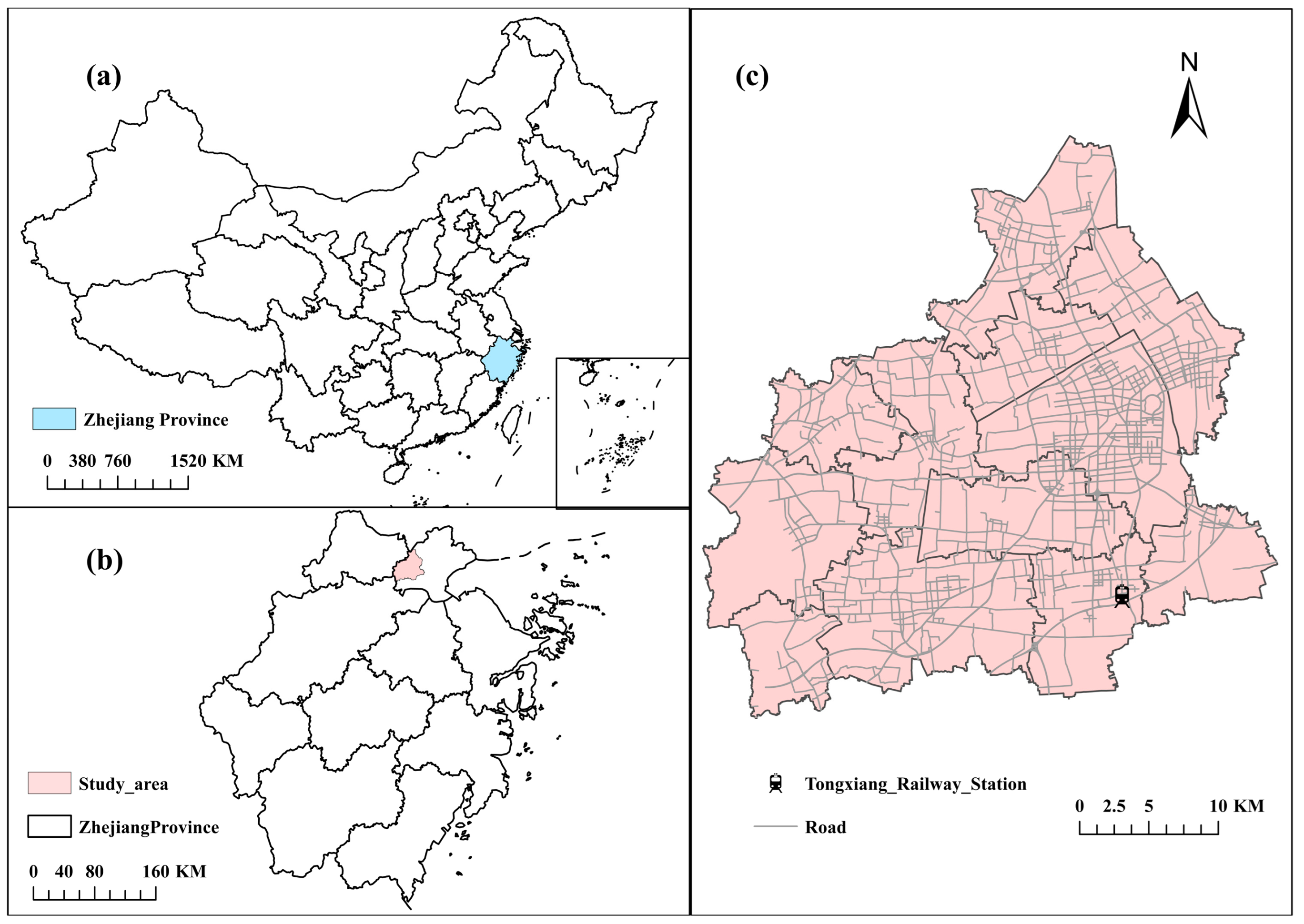
Figure 1. The location of Tongxiang City. (a) The geographical location of Zhejiang Province in China; (b) The geographical location of Tongxiang City in Zhejiang Province; (c) Map of Tongxiang City.
Sustainability 17 10437 g001
Figure 2. Histogram of the distribution of cycling distances.
Sustainability 17 10437 g002
Figure 3. The temporal distribution of cycling demand.
Sustainability 17 10437 g003
Figure 4. Theoretical framework diagram.
Sustainability 17 10437 g004
Table 1. Variable source.
VariablesMain References
Road Network Indicators
Primary roadsChen et al. (2025) [25]
Secondary roadsChen et al. (2025) [25]
Tertiary roadsChen et al. (2025) [25]
Land Use Indicators
Population densityFelix et al. (2025) [26]; Wu et al. (2021) [23]; Chen et al. (2025) [25]
Catering servicesWu et al. (2021) [23]; Chen et al. (2025) [25]; Lang et al. (2023) [18]; Gou et al. (2025) [20]
CorporationsWu et al. (2021) [23]; Chen et al. (2025) [25]; Li et al. (2020) [7]; Shi et al. (2024) [19]
Shopping servicesWu et al. (2021) [23]; Li et al. (2020) [7]; Lang et al. (2023) [18]
Financial servicesLi et al. (2020) [7]; Tang et al. (2024) [22]; Gou et al. (2025) [20]
Culture and educational servicesLi et al. (2020) [7]; Chen et al. (2023) [6]; Gou et al. (2025) [20]
Living servicesLang et al. (2023) [18]; Shi et al. (2024) [19]; Gou et al. (2025) [20]
Sports and leisure servicesGou et al. (2025) [20]; Ma et al. (2020) [17]
Medical servicesChen et al. (2025) [25]; Li et al. (2020) [7]; Tang et al. (2024) [22]; Gou et al. (2025) [20]
Government agencyChen et al. (2025) [25]; Li et al. (2020) [7]; Chen et al. (2023) [6]; Tang et al. (2024) [22]
Accommodation servicesLi et al. (2020) [7]; Lang et al. (2023) [18]; Gou et al. (2025) [20]
Commercial residencesChen et al. (2023) [6]; Tang et al. (2024) [22]
Tourist attractionsChen et al. (2025) [25]; Li et al. (2020) [7]
Public Transport Indicators
Ground public transportWu et al. (2021) [23]; Chen et al. (2025) [25]; Chen et al. (2023) [6]; Tang et al. (2024) [22]
Table 3. Multicollinearity test and spatial autocorrelation test.
VariablesLong-DistanceShort-DistanceSpatial Autocorrelation
Coef.VIFCoef.VIFMoran’s IZ-Scorep-Value
LDT 0.54049.2500.000
SDT 0.46142.7110.000
Shopping services−0.5462.372−1.4732.3590.61656.4130.000
Cultural and educational services9.8791.7194.8071.7040.44040.0940.000
Sports and leisure services10.5352.4508.4832.4470.38435.3570.000
Commercial residences28.7371.75319.2741.7450.60855.0740.000
Accommodation services−1.9211.4932.5781.4950.57453.9340.000
Bus stops29.2611.24242.4171.2460.26323.7770.000
Trunk road density19.0351.13711.2981.1420.39535.7010.000
Table 4. Comparison of fitting effect of OLS, GWR, and MGWR models.
ModelLong-Distance Demand (LDT)Short-Distance Demand (SDT)
AICcR2R2AdjBandwidthAICcR2R2AdjBandwidth
OSL5755.9890.4680.445-5827.0870.3150.285-
GWR962.7240.5550.5033221030.9150.3150.285335
MGWR881.0010.7080.640[68, 423] 949.2380.5790.500[45, 402]
Table 5. Estimation results of MGWR model.
Variables BandwidthMeanStdMinMedianMax
LDTConstant term680.0810.298−0.4180.1290.63
Shopping services2110.2560.0980.0590.2820.377
Cultural and educational services4230.0510.0100.0270.0530.377
Commercial residences4220.1570.0110.1440.1540.183
Sports and leisure services1760.1660.0770.0360.1740.309
Accommodation services423−0.0040.014−0.016−0.0090.052
Bus stops4230.0910.0140.0560.0960.105
Primary road850.0990.225−0.230.0740.746
SDTConstant term450.1040.37−0.520.0351.233
Shopping services2370.1470.085−0.0360.1730.334
Cultural and educational services4020.0330.0110.0020.0350.053
Commercial residences4020.030.0060.0260.0280.051
Sports and leisure services4020.1150.0050.10.1170.121
Accommodation services3380.3660.1270.1440.410.688
Bus stops4020.0880.0110.0580.0920.098
Primary road920.0210.186−0.258−0.0370.523
Disclaimer/Publisher’s Note: The statements, opinions and data contained in all publications are solely those of the individual author(s) and contributor(s) and not of MDPI and/or the editor(s). MDPI and/or the editor(s) disclaim responsibility for any injury to people or property resulting from any ideas, methods, instructions or products referred to in the content.