Article

Empowering Sustainability in Power Grids: A Multi-Scale Adaptive Load Forecasting Framework with Expert Collaboration

1
Shenyang Institute of Computing Technology, Chinese Academy of Sciences, Shenyang 110168, China
2
University of Chinese Academy of Sciences, Beijing 101408, China
3
School of Software Technology, Dalian University of Technology, Dalian 116620, China
*
Author to whom correspondence should be addressed.
Sustainability 2025, 17(23), 10434; https://doi.org/10.3390/su172310434
Submission received: 13 October 2025 / Revised: 8 November 2025 / Accepted: 17 November 2025 / Published: 21 November 2025
(This article belongs to the Special Issue Data-Driven Sustainable Development: Techniques and Applications)

Abstract

Accurate and robust power load forecasting is a cornerstone for efficent energy management and the sustainable integration of renewable energy. However, the practical application of current deep learning methods is hindered by two critical challenges: the rigidity of fixed-length prediction horizons and the difficulty in capturing the complex, heterogeneous temporal patterns found in real-world load data. To address these limitations, this paper proposes the multi-scale adaptive forecasting with multi-expert collaboration (MAFMC) framework. MAFMC’s primary contribution is a novel architecture that utilizes a collaborative ensemble of specialized expert predictors, enabling it to dynamically adapt to complex and non-linear load dynamics with superior accuracy. Furthermore, it introduces an innovative iterative learning strategy that allows for highly flexible, variable-length forecasting without the need for costly and time-consuming retraining. This capability significantly enhances operational efficiency in dynamic energy environments. Extensive evaluations on three benchmark datasets demonstrate that MAFMC achieves state-of-the-art performance, consistently outperforming leading baseline methods and establishing a new standard for power load forecasting.

1. Introduction

The global imperative for sustainable development has reached an unprecedented urgency, driven by the escalating challenges of climate change, finite resource depletion, and pervasive environmental degradation [1,2,3]. This critical juncture demands a paradigm shift towards an intrinsically sustainable future, with the energy sector at its core. Consequently, new-generation sustainable power systems are rapidly emerging, characterized by their high penetration of diverse renewable energy sources such as solar photovoltaics, wind farms, and hydropower, alongside advanced energy storage technologies (e.g., batteries and hydrogen fuel cells), and flexible demand-side management. These systems are inherently decentralized, highly interconnected, and often operate within intelligent grid frameworks (smart grids), leveraging advanced communication and control infrastructure to enhance efficiency, resilience, and adaptability [4,5]. Their design is not merely about generating clean power but encompasses the entire energy value chain, from optimized generation and transmission to intelligent distribution and consumption, all while minimizing ecological footprint and fostering energy equity. This transformative evolution towards decarbonized, resilient, and democratized energy is fundamental to achieving global sustainability goals, opening up vast opportunities for data-driven innovation across interdisciplinary fields, including computer science, information science, applied mathematics, and statistics, to balance environmental, economic, and social imperatives.
Within this complex and dynamic landscape of sustainable power systems, accurate power load forecasting is of paramount importance for enabling efficient energy management and ensuring grid stability, especially given the inherent intermittency and variability of integrated renewable energy sources. The unpredictable nature of renewable generation, coupled with fluctuating demand, significantly amplifies the operational challenges of balancing supply and consumption. Precise load forecasting serves as a critical enabler for more effective planning, scheduling, and real-time operation of these advanced power systems [6]. It directly facilitates the optimal blending of renewable and conventional energy sources, which is crucial for maintaining a reliable and stable power supply while simultaneously maximizing the utilization of clean energy and minimizing reliance on fossil fuels. Furthermore, highly accurate forecasts are indispensable for optimizing the charging and discharging cycles of energy storage systems, which are vital for buffering fluctuations, mitigating peak demand, and ensuring grid resilience against unforeseen disturbances in renewable-dominated grids [7]. Thus, enhancing the precision and adaptability of load forecasting capabilities directly underpins the operational efficiency, economic viability, and ultimately, the long-term sustainability and reliability of our future energy infrastructure.
Current power load forecasting methods primarily encompass machine learning-based methods and deep learning-based methods [8,9]. Machine learning-based methods utilize statistical learning algorithms to extract statistical patterns from historical load data and manually constructed features, e.g., date type and weather [10,11]. They learn the mapping relationships between features and load values to achieve future power load forecasting. However, these methods heavily rely on the quality and effectiveness of manual feature engineering. Furthermore, their capability to capture complex non-linear temporal dependencies, especially long-term dependencies, is limited. Deep learning-based methods employ deep neural network models containing multiple non-linear transformations. They automatically learn deep-level feature representations from raw or minimally processed load and time-series data, capturing complex spatiotemporal dependencies and non-linear patterns to achieve high-precision, end-to-end power load forecasting [12]. With the continuous evolution and iteration of models in the deep learning field, three main branches have emerged as follows: The recurrent neural network (RNN)-based power load forecasting branch utilizes neuron structures with recurrent connections to learn the inherent sequential dependencies within time-series data, which captures short-term dependency information between timesteps to model and forecast sequential data [13]. The long short-term memory (LSTM)-based power load forecasting branch leverages specialized memory unit structures to learn patterns in long-term time-series data. It effectively captures long-term dependencies spanning extended time steps, solving the vanishing/exploding gradient problems inherent in RNNs, thereby enabling more accurate time-series predictions [14]. The transformer-based power load forecasting branch employs the self-attention mechanism to parallelly compute dependencies between all elements in a sequence. It learns global contextual information, capturing long-range dependencies between elements at any positions within the sequence. By abandoning recurrent structures, it achieves efficient and powerful sequence modeling capabilities [15].
Although deep learning-based methods make some progresses in the power load forecasting, there still exist two issues. (1) They typically predefine a prediction head with a fixed length, which severely limits their flexibility and adaptability. In other words, these methods are typically designed to forecast a specific number of future time steps, such as the next hour or day. However, in real-world applications, forecasting needs can vary dynamically due to factors like weather changes, market fluctuations, and sudden demand variations. When the required prediction length changes, the models need to be retrained or redeployed, which is time-consuming and computationally intensive. (2) They generally utilize a single shared linear layer to generate predictions for all data. This approach assumes that all historical time-series data follow the same distribution and pattern, which is unrealistic given the heterogeneous nature of real-world power load data influenced by various factors such as seasonality, weather, and human behavior. Each historical data may have unique characteristics and fluctuation patterns that cannot be adequately captured by a one-size-fits-all linear layer. As a result, the model fails to accurately model the specific distribution and characteristics of each sample, leading to suboptimal power load forecasts.
To this end, this paper proposes a multi-scale adaptive forecasting method (MAFMC) with multi-expert collaboration for mining fluctuate patterns of power load data. Specifically, MAFMC introduces a series patchization strategy via partitioning the power load series into a sequence of non-overlapping patches, which contributes to alleviating the impact of the noise and semantic sparsity hidden in power load series. Then, MAFMC integrates the Transformer network and Kolmogorov–Arnold network [16] into a prediction framework to achieve power load forecasting. The former utilizes the self-attention mechanism to learn and capture long-range dependence between channels. The latter introduces the mixture-of-experts technique to enhance decision adaptability of Kolmogorov–Arnold prediction heads. Meanwhile, MAFMC defines an iterative auto-regressive learning with multi-scale representation extraction via mapping the predicting process into an iterative manner, to replace the current one-step generating paradigm, which can be applied to different prediction lengths without any modification. Finally, numerous experiments are conduced on three real-world datasets and the results show MAFMC sets a new baseline in the power load forecasting task in terms of mean squared error (MSE) and mean absolute error (MAE).
Threefold contributions of MAFMC are as follows:
  • We introduce a pioneering prediction head that integrates a Kolmogorov–Arnold network based mixture-of-experts architecture. This design is specifically engineered to adaptively capture the heterogeneous and often complex distribution and fluctuation patterns inherent in real-world time-series power load data. Unlike traditional linear layers or single-model approaches that assume uniform data characteristics, our MoE-KAN framework leverages the intrinsic flexibility of KANs, which learn univariate functions on their edges—to allow multiple specialized experts to collectively model distinct data sub-patterns. This significantly enhances the model’s capacity to precisely fit diverse non-linear dynamics, thereby leading to superior predictive accuracy and robustness, especially in dynamic and unpredictable power grid environments.
  • We propose an innovative iterative auto-regressive learning mechanism, coupled with multi-scale representation extraction, to enable highly flexible, variable-length prediction generation without the need for arduous retraining. By transforming the prediction process into an iterative loop that progressively refines time-series representations from coarse to fine granularities, our model can dynamically adapt to varying forecasting horizons. This design contrasts sharply with conventional deep learning models that typically predefine a fixed-length prediction head, severely limiting their real-world applicability. Our approach ensures operational efficiency and resource optimization by supporting dynamic forecasting scenarios, a critical requirement for modern, sustainable power grid management.
  • Extensive evaluations conducted on three real-world benchmark datasets, Electricity, NSG-2020, and NSG-2023, consistently demonstrate that MAFMC achieves state-of-the-art performance in power load forecasting. Across various future prediction lengths, our model significantly outperforms six leading baseline methods, evidenced by substantial reductions in MSE and MAE. This empirical superiority underscores the effectiveness of MAFMC’s integrated architecture in addressing the inherent complexities and challenges of power load forecasting, establishing a new benchmark for predictive accuracy and adaptability in this domain.

2. Related Work

2.1. Power Load Forecasting

Power load forecasting methods have evolved from early statistical models like linear regression to artificial neural networks and then to deep learning [17,18,19,20]. Based on the types of input data for the prediction model, power load forecasting methods can be broadly divided into two basic types: one uses historical load data as input to train the power load forecasting model; the other uses historical load data combined with other relevant factors such as meteorological data as input, aiming for the model to uncover the relationships between these factors and historical load values. Since the datasets typically relied upon for power load forecasting generally include historical load data, meteorological data, holiday information, and other external influencing factors, collecting and organizing these multi-dimensional to high-dimensional datasets for training deep learning models can, on the one hand, lead to the curse of dimensionality, reducing the model’s generalization ability. On the other hand, inputting all the raw features without selection into the deep learning model may adversely affect the prediction model’s accuracy and efficiency [21,22,23]. Therefore, feature analysis of historical datasets, precise screening of key feature factors, and reducing data dimensionality become essential. Current research frequently emphasizes the significant importance of accurately screening key feature factors for building prediction models.
Power load forecasting is a typical time-series prediction problem characterized by significant randomness and uncertainty, influenced by numerous external factors such as production schedules, weather conditions, holidays, and unexpected events. Accurately capturing the mapping relationship between feature factors and load data is key to improving the accuracy of short-term power load forecasting. Current short-term power load forecasting techniques can be categorized into traditional time-series learning and deep learning models, or involve building and combining different deep learning model architectures to leverage the strengths of various algorithmic approaches in capturing the temporal characteristics of short-term load sequences. Mainstream deep learning model architectures currently include RNN, CNN, LSTM, and Attention [24,25]. Considering the differences among various deep learning network architectures in terms of their ability to understand time sequences, reasoning capability, convergence speed, and prediction accuracy, some works proposes several network architecture splicing schemes [1,6,7]. These spliced hybrid models can improve prediction capability to a certain extent. However, combined models suffer from issues like cumulative dimensionality increase, proliferation of hyperparameters, and increased training complexity, leading to poor model convergence and hindering real-time application.
Power load forecasting has now entered the era of big data, making it possible to utilize multi-dimensional datasets to build powerful deep learning models to solve complex system short-term load forecasting. For instance, the deep Informer model, developed based on the classic Transformer architecture, has attracted significant attention due to its ability to capture long-term sequence features, fast inference speed, and high accuracy. Preliminary studies have shown the effectiveness of the Informer model in various long-term time-series forecasting tasks. For example, Gong et al. [26] integrated breadth-first search, GRU networks, and Informer to construct a hybrid GruDA-Informer model. It jointly modeled multi-dimensional datasets at different time scales and combined the prediction results, significantly increasing the model’s complexity. Ma et al. [27] utilized deep wavelet transform for dataset feature engineering, formulating a feature set input for the deep learning prediction model. By predicting the load curve over the model’s window period and interval, they effectively improved short-term power load forecasting accuracy. Liu et al. [28], combining the concept of variational mode decomposition, established several independent Informer models for different modes. While these multi-modal models address the issue of information increment between modalities, training them solely on multi-modal historical load data results in limited generalization ability, making it difficult to accurately capture the uncertainty of short-term load change trends.
Despite these advancements, current hybrid deep learning models, such as those integrating Informer or GruDA-Informer architectures, often face limitations in terms of fixed prediction horizons, inherent architectural rigidities, and an inability to dynamically adapt to heterogeneous data patterns without extensive retraining. Many existing methods still rely on a single, shared prediction head, implicitly assuming a uniform distribution across diverse time-series data, which is an oversimplification for real-world power loads. In contrast, our proposed MAFMC fundamentally addresses these challenges by introducing a novel KAN-based mixture-of-experts prediction head, enabling adaptive modeling of distinct data characteristics. Furthermore, its iterative auto-regressive learning mechanism facilitates flexible, variable-length forecasting, a significant departure from the fixed-horizon predictions prevalent in prior works. This architectural paradigm shift allows MAFMC to achieve superior adaptability and robustness, providing a more versatile and accurate solution for sustainable power grid management.

2.2. Kolmogorov–Arnold Networks

The Kolmogorov–Arnold representation theorem states that any multivariate continuous function can be precisely decomposed into a finite composition of univariate continuous functions and the addition operator [16]. Inspired by this, the Kolmogorov–Arnold Network (KAN) was proposed as a revolutionary alternative architecture to the traditional multilayer perceptrons (MLPs). Unlike MLPs, which apply fixed, often monotonic activation functions, e.g., ReLU and Sigmoid, at neuron nodes, KAN shifts the learnability to the network connecting edges. This design endows KAN with exceptional flexibility in function representation and adaptability to complex data patterns, theoretically enabling it to approximate high-dimensional functions more efficiently and accurately. Consequently, KAN is considered a highly promising alternative to MLPs.
The original KAN implementation relied on spline functions to parameterize the learnable univariate functions on its edges. This created bottlenecks in the training and inference speed of the original KAN, limiting its scalability for large-scale data and deep networks. To overcome this limitation, subsequent research focused on finding computationally more efficient and lightweight basis function alternatives. For example, ChebyshevKAN introduced Chebyshev polynomials as basis functions, which significantly boost KAN’s computational speed [29]. Another representative work is FastKAN, which innovatively employs Gaussian radial basis functions to approximate the cubic B-splines used in the original KAN [30]. Gaussian RBFs are extremely efficient to compute (primarily involving exponentiation) while providing sufficient expressive power, resulting in significantly faster runtime compared to the original spline-based KAN while maintaining comparable accuracy. This greatly enhances the practicality of KANs.
KAN architecture is rapidly being explored and applied across diverse fields beyond foundational research. In computer vision, Convolutional KAN emerged, discarding the concept of linear filters in traditional convolutional layers [31]. Instead, it uses matrices composed of learnable spline functions to perform convolution, aiming to capture complex spatial patterns and features in images more flexibly. In medical image analysis, U-KAN [32] successfully integrated KAN layers into the classic U-Net segmentation architecture, replacing some or all MLP layers. Research like physics-informed KAN [33] and KAN variants of physics-informed neural networks [34] utilize KANs to build physics-informed machine learning models. By directly encoding physical laws as constraints within the network structure or loss function, these models significantly improve interpretability, generalization capability, and data efficiency in scientific computing and engineering simulation domains. It is within this context that we aim to introduce KAN into the critical field of electricity load forecasting. We are committed to exploring and validating KAN’s exceptional potential in effectively representing the complex spatiotemporal dependencies and non-linear dynamic patterns inherent in electricity load data, with the goal of enhancing prediction accuracy and model interpretability.

3. The Proposed Method

Considering the input series of the power load X R C × L where C denotes the number of channels and L denotes the history window length, the goal of the power load forecasting is accurately predicting future series values Y R C × H where H denotes prediction window length. To achieve the above goal, we propose a multi-scale adaptive power load forecasting method with multi-expert collaboration (MAFMC), which consists of the input series patchization, multi-expert adaptive prediction, and iterative auto-regressive learning, as shown in Figure 1.

3.1. Input Series Patchization

To alleviate the impact of the noise and semantic sparsity hidden in power load series, a series patchization strategy is devised via partitioning the input series into a sequence of non-overlapping patches, which contributes to achieving precise power load forecasting.
Specifically, we partition the input series X R C × L of the power load into non-overlapping patches x ˜ R C × N × T , where N × T = L , N and T denote the number and length of patches, respectively.
x ˜ i = { x ˜ ( i 1 ) T + 1 , x ˜ ( i 1 ) T + 2 , , x ˜ i T } , i = 1 , 2 , , N
where x ˜ i denotes the i-th patch of the input series. Moreover, there exists a distribution shift in time-series data, characterized by changes in the mean and variance over time. To this end, a normalization operation is introduced to mitigate the distribution shift:
x i = x ˜ i μ i σ i + ϵ , ϵ > 0
μ i = 1 T t = 1 T x ˜ t i
σ i = 1 T t = 1 T ( x ˜ t i μ i ) 2
where ϵ is a small constant to prevent division by zero. Then, the non-overlapping patches { x i } i = 1 N are input to the model to obtain the power load forecasting.

3.2. Multi-Expert Adaptive Prediction

Multi-expert adaptive prediction consists of a circular Transformer block and an adaptive KAN-based time-series predictor. The former aims to capture long-range dependence between channels via the self-attention mechanism and the latter dynamically learns power load fluctuation patterns with the help of the mixture-of-experts technique.
Specifically, given the i-th patch x i , MAFMC performs a max-pooling operation for down-sampling into x i n i R C × N × T / k where k denotes the convolutional kernel size, and then utilizes a circular Transformer block to obtain the corresponding time-series representations. The process of the b-th block is defined as follows:
h ˜ b i = P E ( h b 1 i ) + R E ( h b 1 i )
h ^ b i = W o ( A t t e n t i o n ( W q h ˜ b i , W k h ˜ b i , W v h ˜ b i ) + h ˜ b i
h b i = F F N ( h ^ b i ) + h ^ b i
where b = 1 , 2 , , B . P E ( · ) and R E ( · ) denote position and feature projections, respectively. W o , W q , W k , and W v denote the linear projections. h 0 i = x i n i . A t t e n t i o n ( · ) and F F N ( · ) denote a multi-head cross-attention and a feed-forward network, respectively.
After obtaining representations h B i , tradition methods utilize a simple linear projection function W y to obtain future prediction y p r e d , which can be defined as follows:
y p r e d = W y ( z i ) + b y
where b y is weighting bias z i = h B i . There exist two limitations: (1) Real-world time-series power grid data often exhibit complex non-linear patterns including periodicity, trends, and random fluctuations. The above prediction strategy, constrained by their inherent linear nature, struggle to effectively capture these intricate non-linear relationships, thereby limiting forecasting accuracy. (2) Different channels may possess distinct statistical properties and distributions. The above prediction strategy, through the adoption of uniform linear transformations for all channels, lack the flexibility to tailor adjustments according to the specific characteristics of each channel, making them poorly suited to adapt to the inherent diversity among the channels.
Inspired by the flexibility of Kolmogorov–Arnold networks, we propose an adaptive time-series predictor via integrating various KAN variants into the mixture-of-experts framework to address the above limitations. Each expert is implemented via KAN with distinct basis functions, such as B-splines, wavelets, Taylor polynomials, and Jacobi polynomials. These basis functions let each expert excel in capturing specific data distributions and patterns. For instance, wavelet-based KAN expert is great for transient features, while spline-based KAN expert is better for stationary trend modeling.
KAN expert:The adaptive time-series predictor comprises M KAN experts. The m-th KAN expert with U layers can be represented as
Φ m ( z i ) = Φ U Φ U 1 Φ 1 ( z i )
where Φ u , u = 1 , 2 , , U denote a KAN layer with output dimensions [ n 1 , n 2 , , n u ] . The calculation process for each feature in the KAN layer can be expressed as
z u , j i = o = 1 n u 1 Φ u 1 , j , o ( z u 1 , o i )
Different KAN expert defines distinct Φ :
Φ ( z i ) = Residual ( z i ) + Base ( z i )
where Residual ( · ) denotes the residual activation function. Base ( · ) denotes the generalized base functions.
We select B-splines, wavelets, Taylor polynomials, and Jacobi polynomials as different base functions to conduct KAN experts. The reasons are as follow: B-splines offer excellent flexibility and smoothness, making them particularly well suited for modeling underlying trends and stationary, slowly varying components often observed in load profiles. Their local support property also contributes to robustness against localized noise. Wavelets, conversely, are highly effective at capturing transient features, sudden changes, and multi-frequency components within the data, which are characteristic of unexpected events or rapid fluctuations in power demand. Their ability to localize features in both time and frequency domains makes them invaluable for detecting short-lived anomalies. Taylor polynomials provide a robust means of approximating continuous functions locally, enabling the KAN experts to model smooth, predictable changes in load behavior over specific intervals. Finally, Jacobi polynomials, as orthogonal polynomials, offer a systematic way to represent functions with varying degrees of smoothness and can efficiently approximate a wide range of continuous functions, contributing to the model’s overall versatility and robustness in handling diverse and complex load dynamics.
Expert collaboration: We employ a gating network to dynamically assign time-series power load data to the most suitable KAN experts, which determines the weight of each expert via the following formula:
G m ( z i ) = exp ( W m z i ) j = 1 M exp ( W j z i )
where exp ( · ) denotes the exponential function and W m is a learnable weight matrix. Then, we aggregate the outputs of the KAN experts through the decision-making weight of each expert. The aggregation process is
y p r e d = U p S a m p l i n g ( m = 1 M G m ( z i ) Φ m ( z i ) )
where y p r e d denotes future prediction via the adaptive time-series predictor. U p S a m p l i n g ( · ) is an up-sampling operation corresponding to down-sampling operation.

3.3. Iterative Auto-Regressive Learning

Real-world time-series often exhibit diverse periodicities and patterns, such as short-term fluctuations, long-term trends, and seasonal variations. Features at different scales play distinct roles in the power load scenario. To this end, we introduce an iterative auto-regressive learning mechanism that models a progressive, coarse-to-fine extraction of time-series representations.
Specifically, we construct S-cascaded multi-expert adaptive prediction stages (in our experiments, S = 4 ). Each stage is designed to capture features at a specific temporal scale, controlled by sequentially defined down-sampling kernels (e.g., 8, 4, 2, and 1). This architecture enables the model to gradually capture features from global trends to local details, enhancing both accuracy and adaptability. To ensure that each subsequent stage focuses on refining the prediction, we employ a residual learning principle. The prediction target for each stage is the remaining error from the previous stages. This is formalized as follows: let y i + 1 be the ground-truth for the next patch. The target for the first stage ( s = 1 ) is y i + 1 . The target for a subsequent stage s > 1 is the residual y i + 1 k = 1 s 1 y ^ k , pred i , where y ^ k , pred i is the prediction from stage k.
The final prediction for the next patch is the sum of the outputs from all S stages. After this aggregation, the result is de-normalized using the reversed instance normalization operation to produce the final prediction in the original data scale. Let y ^ s , pred i denote the output of the s-th stage for the i-th sample. The final prediction y ^ i + 1 is obtained by
y ^ i + 1 = s = 1 S y ^ s , pred i · ( σ i + ϵ ) + μ i .
where μ i and σ i are the mean and standard deviation of the input patch x i , respectively.
The model is trained to minimize the discrepancy between this final prediction y ^ i + 1 and the ground-truth next patch y i + 1 . For this optimization, we utilize the Huber loss, which combines the benefits of mean squared error (MSE) and mean absolute error (MAE). The loss function L for a single sample is formally defined as
L ( y ^ i + 1 , y i + 1 ) = 0.5   ×   y ^ i + 1 y i + 1 2 2 if y ^ i + 1 y i + 1 1 < δ δ · y ^ i + 1 y i + 1 1 0.5 · δ otherwise
where y i + 1 denotes the true values of the next patch, · denotes a vector norm, and δ is the threshold parameter, which we set to 1 in our experiments. The total loss for a training batch is the average of this value across all samples. The advantage of Huber loss is threefold. Firstly, it is less sensitive to outliers than MSE. When the prediction error is small, it behaves like MSE, allowing for stable convergence. When the error is large, it behaves like MAE, preventing the large gradients that can destabilize training. Secondly, its smoothness at the threshold ensures a stable optimization process. Finally, this robustness is particularly beneficial for accurately capturing patterns in noisy time-series data, thereby improving overall prediction accuracy.
For inference, the trained model predicts the next patch in an auto-regressive manner. Given an input series, the model first predicts the subsequent patch. This predicted patch is then appended to the input series to predict the next one, and this process is repeated until the desired forecast horizon is reached. To manage computational costs, only the most recent N p patches are used as input for prediction. In our experiments, the patch length T and the number of input patches N p are set to 48 and 7, respectively.

3.4. Theoretical Analysis of MAFMC

In this chapter, we theoretically demonstrate the superiority of the MAFCM framework in power load forecasting, including (1) the optimization benefits of the Mixture-of-Experts KAN architecture for heterogeneous data, (2) the role of patch-wise normalization in improving generalization under distributional shifts, and (3) the functional decomposition advantage of iterative residual learning.

3.4.1. Optimization of Expected Loss on Heterogeneous Distributions

Let the power load data be drawn from a distribution p ( X , Y ) , where X R C × L is the input series and Y R C × H is the prediction series. In generally, power load data follows the complex and heterogeneous distributions with a mixture of distinct patterns (e.g., weekday vs. weekend cycles, seasonal trends, and stochastic fluctuations from renewable energy integration). Thus, we posit that the distribution is a mixture of M underlying simpler distributions, corresponding to different operational regimes. Formally, as follows:
p ( X , Y ) = k = 1 M P ( k ) p k ( X , Y )
where k { 1 , , M } is a latent variable representing the regime, and P ( k ) is the prior probability of that regime. The goal of the power load forecasting is to find a function f that minimizes the expected loss, typically the mean squared error: L ( f ) = E ( X , Y ) p Y f ( X ) 2 .
The conventional single monolithic model, f single , must find a single set of parameters θ to minimize this loss across all regimes:
L ( f single ) = k = 1 M P ( k ) E ( X , Y ) p k Y f single ( X ) 2
The optimal function f single * is a compromise, attempting to fit all M distributions simultaneously. This can lead to a high irreducible error if the optimal predictors for each regime, f k * = arg min f E p k [ Y f ( X ) 2 ] , are substantially different.
The multi-expert adaptive prediction of MAFMC approximates the predictor as f map ( X ) = m = 1 M G m ( X ) f m ( X ) , where f m are the KAN experts and G m ( X ) is the gating network’s output, designed to approximate the posterior probability P ( m | X ) . The expected loss is
L ( f map ) = E X [ E Y | X [ Y m = 1 M G m ( X ) f m ( X ) 2 ] ]
Assuming the gating network is sufficiently powerful such that G m ( X ) δ m , m * ( X ) where m * ( X ) is the true underlying regime for input X and δ is the Kronecker delta, the loss function approximately decomposes the following:
L ( f map ) m = 1 M P ( m ) E ( X , Y ) p m [ Y f m ( X ) 2 ]
This decomposition demonstrates a critical advantage: each expert f m can specialize in minimizing the loss for its corresponding data distribution p m , unburdened by the need to fit other regimes. The overall minimum achievable loss is therefore P ( m ) L ( f m * ) , which is provably less than or equal to the loss achievable by the single model, L ( f single * ) . This mathematical decomposition provides a formal justification for the MoE-KAN’s superior ability to model complex, heterogeneous data.

3.4.2. Generalization Under Covariate Shift via Normalization

The non-stationarity of time-series data implies that the distribution of input patches changes over time. Let X i and X j be two patches from different time steps. Non-stationarity means their distributions p i ( X ) and p j ( X ) are different, i.e., p i p j . This is a classic example of covariate shift, a major challenge for model generalization.
Let the mean and standard deviation of patch X i be μ i and σ i . Our instance normalization applies a transformation T i ( X i ) = X ^ i = ( X i μ i ) / σ i . By definition, the transformed patch X ^ i has a distribution p ^ i with E [ X ^ i ] = 0 and Var [ X ^ i ] = I . While higher-order moments might still differ, this transformation stabilizes the first two moments of the input distributions across all patches.
From the perspective of statistical learning theory, generalization bounds (e.g., based on VC dimension or Rademacher complexity) depend on the similarity between the training and test distributions. By applying the transformation T, we are actively minimizing the discrepancy between the distributions of different patches. The model f map trained on the normalized data { X ^ i } faces a learning task with a significantly reduced domain shift. It follows that f map is expected to have a tighter generalization bound and thus perform more robustly on unseen data compared to a model trained on the original, non-stationary data.

3.4.3. Optimization Simplification via Iterative Residual Decomposition

Let the desired mapping be Y = f map * ( X ) . A standard end-to-end model attempts to learn f map * directly by optimizing parameters θ for a model f ( X ; θ ) . The optimization landscape for this direct mapping may be highly complex and non-convex. MAFMC approximates f map * as a sum of functions learned in stages: f map ( X ) = s = 1 S f map s ( X ) . The learning process is defined recursively as follows:
  • Stage 1: Y 1 arg min f E [ Y f map 1 ( X ) 2 ]
  • Stage s: Y s arg min f E [ ( Y j = 1 s 1 f map s 1 ( X ) ) f map s ( X ) 2 ]
Let R s = Y j = 1 s 1 f map s 1 ( X ) be the residual before stage s. The task at stage s is to model this residual. This formulation is mathematically analogous to function-space gradient descent, as employed in gradient boosting. Each function f map s represents a step in the function space that greedily minimizes the overall loss.
This decomposition offers a significant optimization advantage. Consider the case where f map * ( X ) = H ( X ) + R ( X ) , where H ( X ) is a simple, low-frequency component and R ( X ) is a complex, high-frequency one. The first stage, f map 1 , can easily capture the dominant component H ( X ) . Subsequent stages, f map 2 , , f map S , are then free to dedicate their entire capacity to fitting the more complex residual R ( X ) . By breaking down a single, complex optimization problem into a sequence of simpler ones, the model is guided through a more stable optimization trajectory, reducing the risk of converging to a poor local minimum and enabling a more accurate approximation of the true function f map * .

4. Experiment

4.1. Setup

Datasets and Metrics: Three real-world datasets [11] are used as benchmarks to evaluate power load prediction performance of MAFMC, i.e., Electricity, NSG-2020, and NSG-2023, whose detailed statistical information are provided in Table 1. Following current methods, the dataset is divided into 60% training subset, 10% validation subset, and 30% testing subset datasets. The NSG-2020 and NSG-2023 datasets are collected from the Northeast China National Grid, which covers the power load profiles of Liaoning, Jilin, Heilongjiang, and eastern Inner Mongolia provinces. These datasets capture high-frequency (15 min interval) electricity-demand measurements spanning 2020 and 2023, respectively, and are curated by the China Electric Power Research Institute (CEPRI) to reflect the region’s distinctive seasonal, industrial, and residential load characteristics. Due to data-usage licensing agreements, the datasets are not publicly available at present; however, the authors have committed to releasing them upon formal acceptance of the manuscript, subject to approval by CEPRI. Researchers interested in accessing the data may submit a formal request to the corresponding author, who will facilitate the necessary permissions and provide the datasets in CSV format with standardized time-series aggregation. This controlled-release approach ensures compliance with China’s power-sector data-security regulations while enabling reproducible, high-quality research on regional load-forecasting challenges. The MSE and MAE are used as metrics to measure power load prediction performance of MAFMC.
Implementation Details: MAFMC uses Python 3.6.10 with PyTorch 2.0 to implement the overall network and run on the GPU server with NVIDIA A100. In the experiments, MAFMC contains four cascaded multi-expert adaptive prediction stages. Each stage consists three cascaded Transformer blocks and an adaptive time-series predictor. The convolutional kernel sizes of down-sampling operation in each stage are set as 8, 4, 2, and 1, respectively. The optimizer uses Adam with the learning rate 0.0001, the epoch number 100, and the batch size 32 for three datasets. An early stopping strategy is used to prevent overfitting and ensures the model achieves the best possible generalization on unseen data. Specifically, the training process is monitored based on the validation loss. If the validation loss does not show any improvement for 10 consecutive epochs (a patience of 10), the training was automatically halted. The codes and datasets are publicly available at https://github.com/Machinelearning20/MAFMC (accessed on 1 November 2025).
Comparison methods: Eight power load forecasting methods are utilized as comparison methods, which can be partitioned into two classes, i.e., time-series common forecasting methods and time-series power load forecasting methods. The former includes TimeCMA (2025, AAAI) [35], TimeKAN (2025, ICLR) [36], Informer (2021, AAAI) [37], and FEDformer (2022 ICML) [38]. The latter contains hybrid-LT (TSG, 2025) [1], LDTformer (ESWA, 2024) [3], ConvLSTM (ESWA, 2024) [7], and MTMV (EPSR, 2023) [24]. To ensure the fairness of the comparison, the following measures are adopted. The input series length is standardized to 336 for all baselines to maintain consistency in the data input dimensions across different models. Hyperparameters for each method are carefully tuned to optimal settings based on validation sets to ensure that each model can perform to the best of its ability.

4.2. Performance Comparison

Table 2 shows the comparison results on three power load forecasting datasets in terms of MSE and MAE. It can be observed that MAFMC obtains the best forecasting results in comparison with eight methods in terms of five future prediction lengths. For example, MAFMC achieves the lowest error values across the mean of the three datasets in terms of both MSE and MAE, showing significant superiority over the other methods. The reasons are twofold: The multi-expert collaborative prediction head, based on KAN, can adaptively fit the complex distribution and fluctuation patterns of time-series power load data. Unlike traditional methods that use a single shared linear layer, this approach leverages different KAN experts specialized in capturing specific data distributions and patterns. Additionally, the iterative auto-regressive learning strategy enables the model to generate predictions for different lengths without retraining. In contrast to many existing deep learning methods that have a fixed prediction length, this strategy maps the prediction process into an iterative manner, making the model highly flexible and adaptable to dynamic forecasting scenarios. It also incorporates multi-scale representation extraction, allowing the model to capture features from global trends to local details progressively. This is particularly beneficial for handling time-series data with diverse periodicities and patterns, such as short-term fluctuations, long-term trends, and seasonal variations. As a result, the MAFMC method can provide more accurate and reliable power load forecasts, setting a new benchmark in the field. Meanwhile, as shown in Table 2, the state-of-the-art time-series common forecasting methods, i.e., TimeCMA and TimeKAN, achieve much better results in power load forecasting than time-series power load forecasting methods, i.e., hybrid-LT, LDTformer, ConvLSTM, and MTMV. This shows that it is effective and necessary to introduce advanced AI frameworks and algorithms into the power load forecasting field. In other words, applying advanced general time-series forecasting methods to power load forecasting can significantly improve its performance, which fully demonstrates the great potential and value of integrating cutting-edge AI technologies in this specific domain.
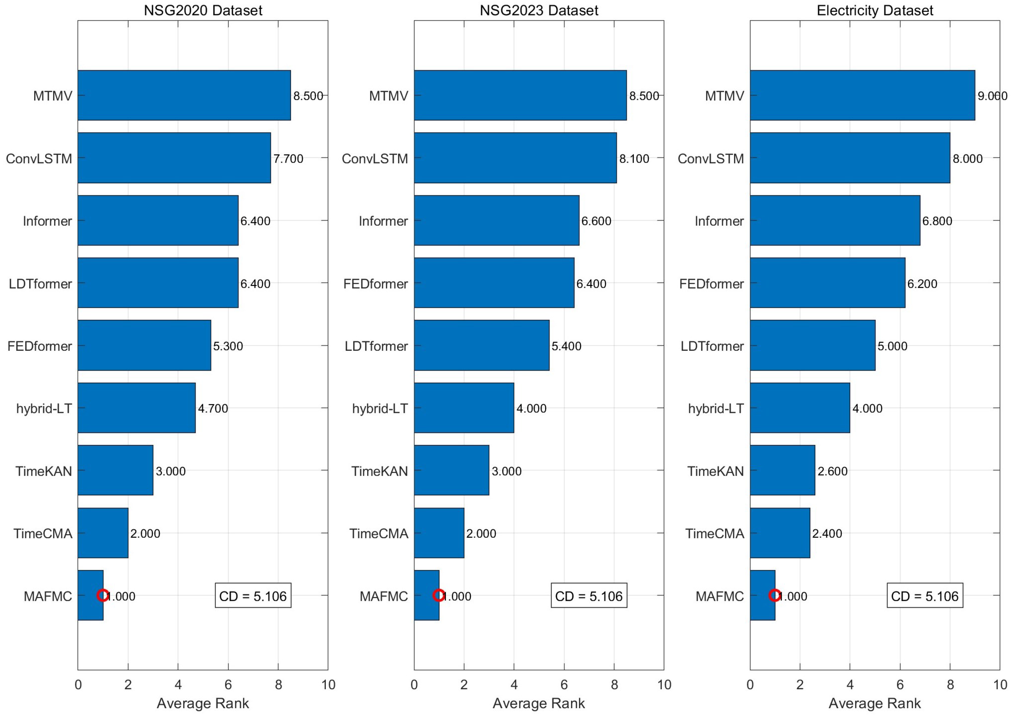
Furthermore, to rigorously validate these findings from a statistical standpoint, we conduct the Nemenyi test on all methods across the three power load forecasting datasets. The Nemenyi test is a post hoc test used after a Friedman test to compare the average ranks of different methods and determine if their performance differences are statistically significant. The results are visualized in the Critical Difference (CD) diagram shown in Figure 2. In this diagram, methods are plotted on an axis according to their average rank, with the best-performing methods having the lowest rank. A thick horizontal bar represents the Critical Difference; any two methods connected by this bar are considered to have a performance that is not statistically different from each other. As the diagram clearly illustrates, our proposed MAFMC achieves the best (lowest) average rank. This provides strong statistical evidence that the superiority of MAFMC is not due to random chance, but rather a significant and consistent improvement over the existing state-of-the-art.

4.3. Ablation Study

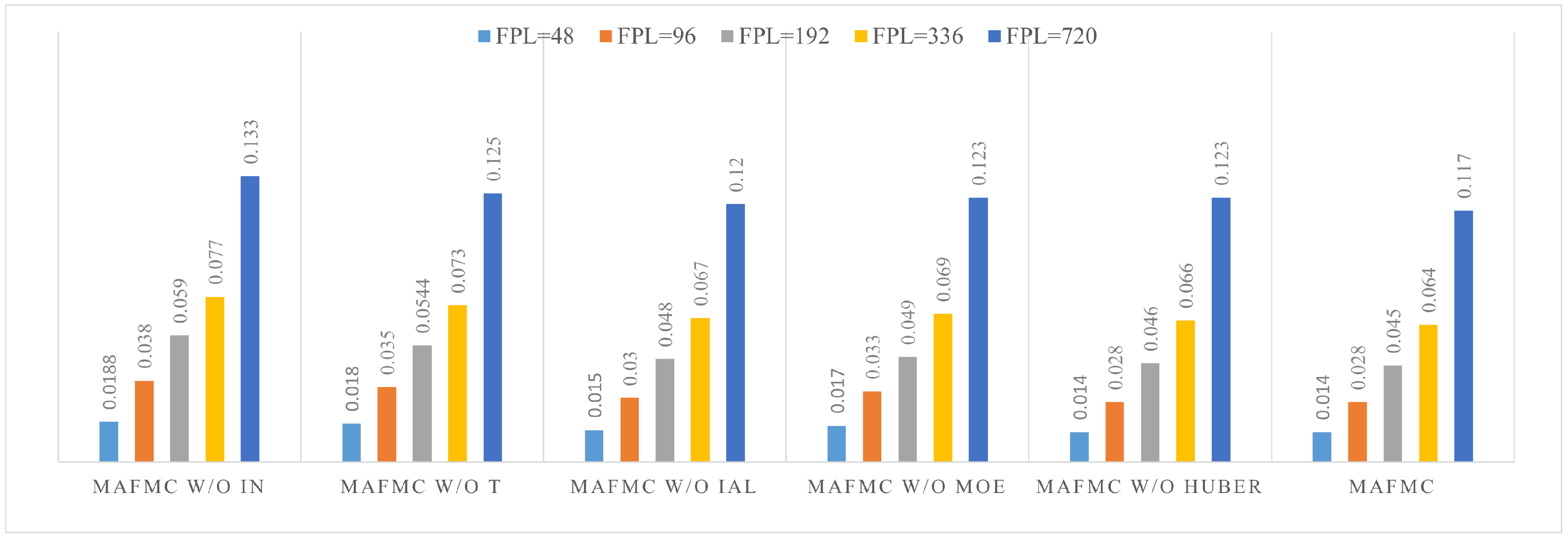
The ablation study is conducted to test the impact of components in MAFMC on the power load prediction performance. Specifically, there are five variants:
  • MAFMC w/o IN denotes the excision of the instance normalization.
  • MAFMC w/o T denotes the excision of Transformer. This variant directly uses KAN-based mixture-of-experts to generation prediction results.
  • MAFMC w/o IAL denotes the excision of the iterative auto-regressive learning.
  • MAFMC w/o MOE denotes the excision of KAN-based mixture-of-experts. This variant uses traditional linear layer as the predictor.
  • MAFMC w/o Huber denotes the excision of the Huber loss. This variant uses traditional MSE as the optimization loss.
The ablation study results presented in Figure 3 offer valuable insights into the contributions of various components within the MAFMC model. When instance normalization (IN) is removed (MAFMC w/o IN), there is a noticeable decline in performance, indicating its significance in stabilizing and accelerating the training process by normalizing the inputs to each patch, which helps in mitigating the distribution shift and improving the model’s generalization ability. The absence of the Transformer block (MAFMC w/o T) leads to a substantial drop in accuracy, underscoring the crucial role of the Transformer in capturing long-range dependencies across channels through its self-attention mechanism, which is vital for understanding the complex temporal patterns in power load data. Removing the iterative auto-regressive learning (IAL) component (MAFMC w/o IAL) also results in inferior performance, demonstrating that the iterative approach effectively extracts multi-scale features and enhances the model’s adaptability to different prediction lengths and time-series patterns. The variant without the KAN-based mixture-of-experts (KAN-MOE) (MAFMC w/o MOE) shows a significant decrease in prediction accuracy, highlighting the superiority of the MOE in modeling the complex non-linear relationships and diverse distribution patterns in power load data compared to traditional linear layers. Lastly, replacing the Huber loss with MSE (MAFMC w/o Huber) affects the model’s robustness, especially in the presence of outliers, as the Huber loss combines the benefits of MSE and MAE, making the training process more stable and the model more capable of handling noisy data. These observations collectively emphasize the importance of each component in the MAFMC model and validate the effectiveness of the proposed method for power load forecasting.

4.4. Parameter Study

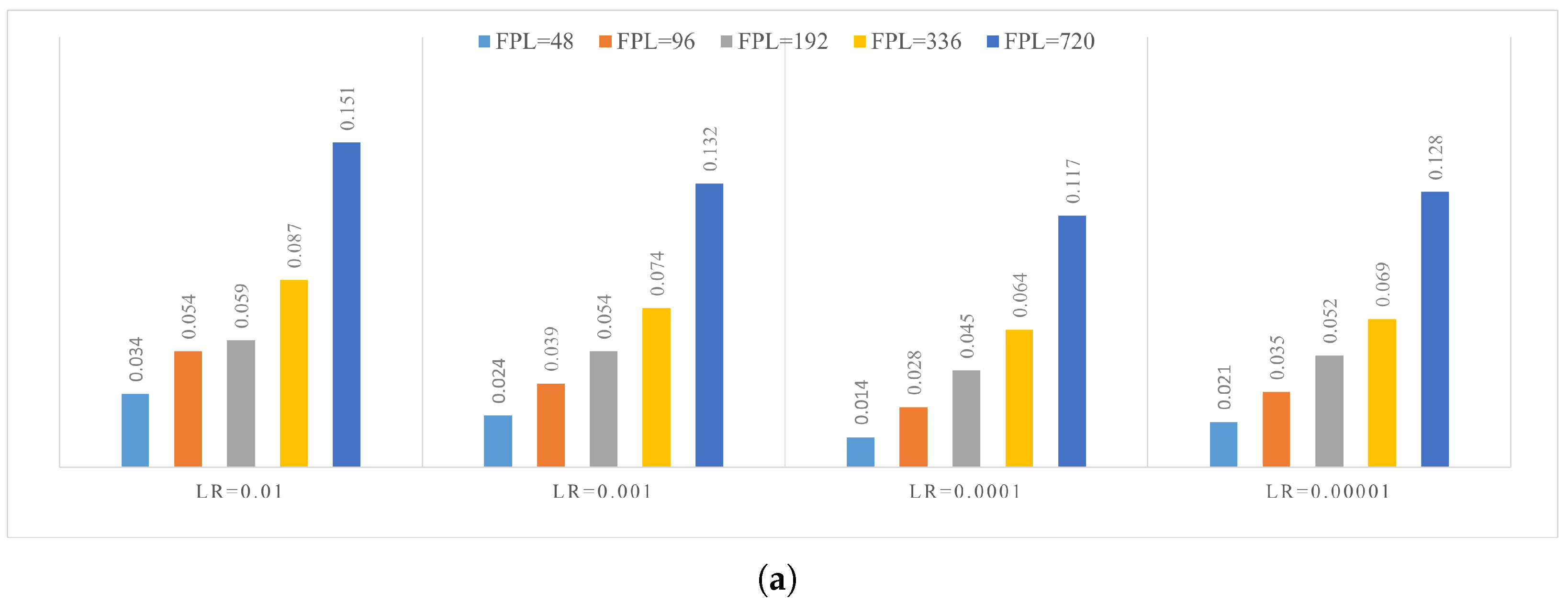
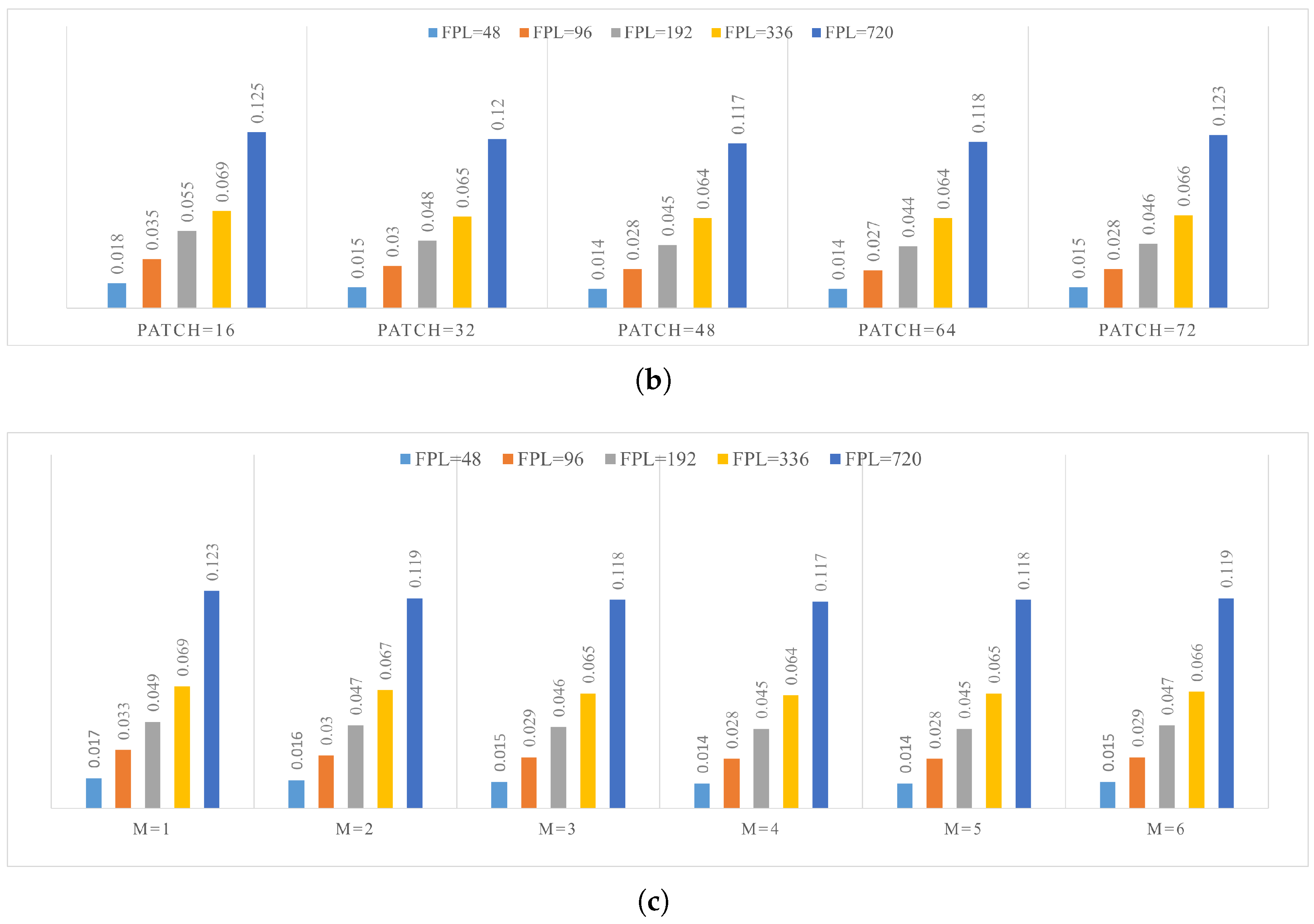
To assess the robustness and sensitivity of the proposed MAFMC model, we conducted a comprehensive hyperparameter sensitivity analysis focusing on three critical parameters: the learning rate, patch size, and the number of experts in the mixture-of-experts (MoE) module. The analysis reveals that the model exhibits stable performance across a reasonable range of values, though optimal results are achieved with specific settings, as shown in in Figure 4. For the learning rate, values significantly higher than 0.0001 led to training instability and convergence issues, while lower values resulted in unnecessarily prolonged training without performance gains; thus, 0.0001 was identified as the optimal balance between convergence speed and stability. Regarding the patch size, smaller patches struggled to capture sufficient temporal context, whereas larger patches introduced noise and reduced granularity, confirming 48 as the ideal length for effectively segmenting the load series while preserving meaningful patterns. Finally, varying the number of experts demonstrated that fewer than four experts limited the model’s capacity to capture diverse load dynamics, while more than four introduced redundancy and increased computational cost without significant accuracy improvements. These findings validate that the selected hyperparameters, i.e., learning rate of 0.0001, patch size of 48, and expert number of four, collectively ensure robust and efficient model performance across varying forecasting scenarios.

4.5. Input Length Study

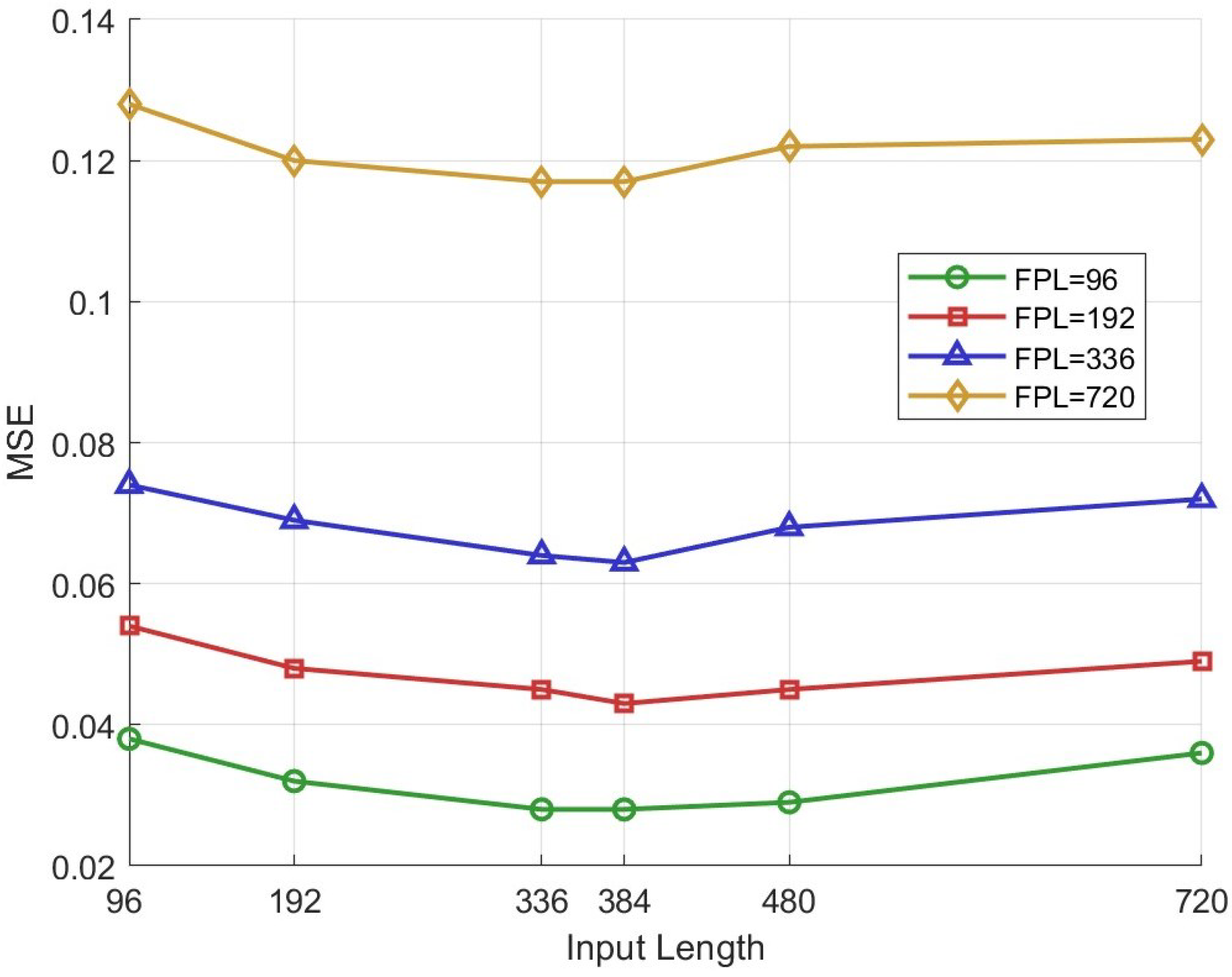
In our input length study across various input lengths (96, 192, 336, 384, 480, and 720), we observed that as the input length increases, the model’s performance generally improves, with MSE values decreasing for all forecast horizons. As shown in Figure 5, for the 96-step forecast horizon, MSE decreases from 0.038 at input length 96 to 0.028 at 336, then stabilizes. Similarly, for the 720-step forecast horizon, MSE decreases from 0.128 at 96 to 0.117 at 336, with minimal improvement beyond that. However, longer input sequences also lead to increased computational costs, including longer training time, higher memory requirements, and slower inference speed. After careful evaluation, we selected an input length of 336 as the optimal balance. This choice provides near-maximal performance benefits while avoiding the diminishing returns seen in longer sequences. It also ensures suitable computational efficiency for real-time applications and maintains backward compatibility with typical data collection window sizes.

4.6. Convergence Study

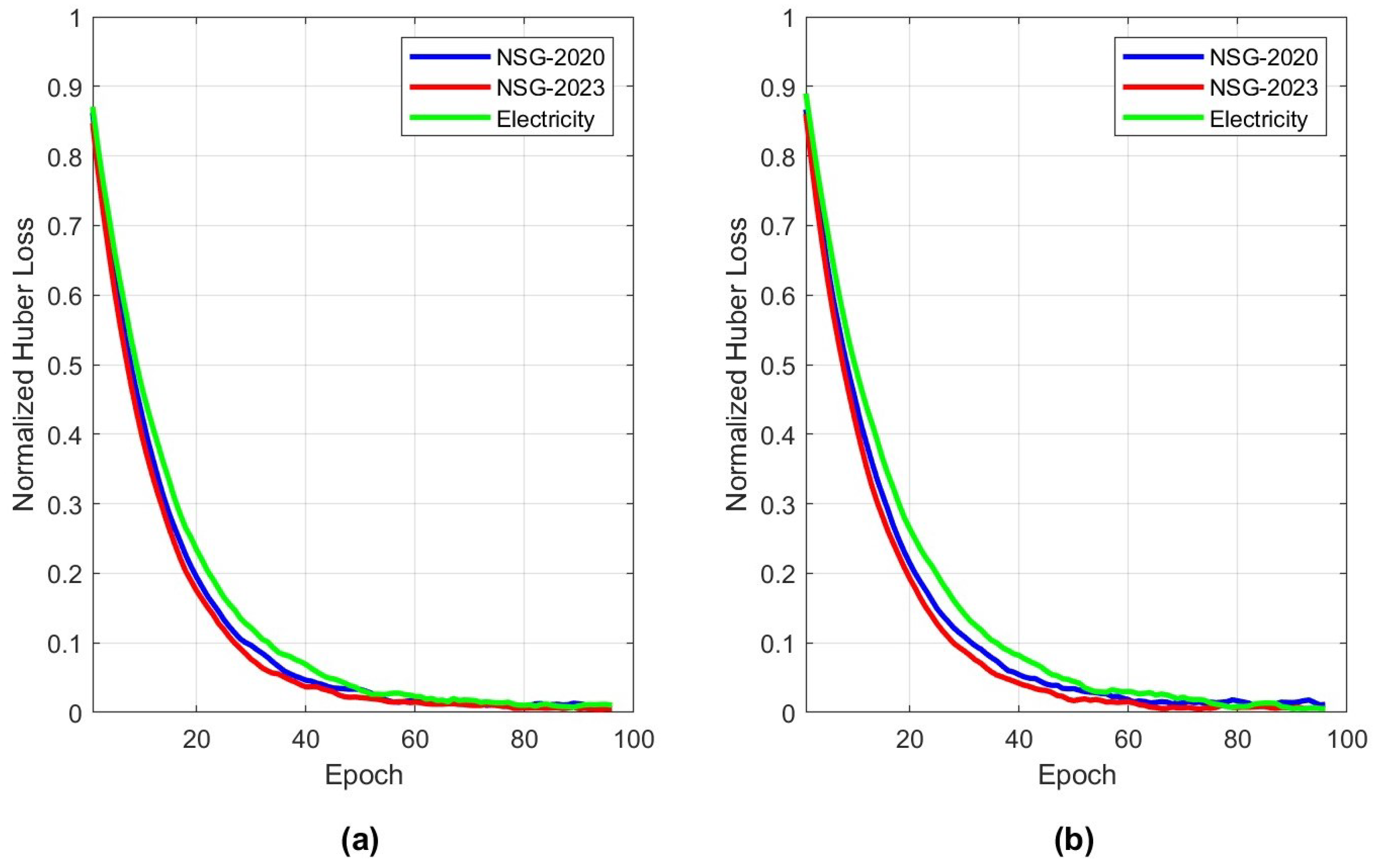
To comprehensively demonstrate the training stability and generalization capability of the proposed MAFMC framework, we present a detailed convergence analysis by monitoring both training and validation losses across all three benchmark datasets. Figure 6 illustrates the normalized Huber loss trajectories throughout the 100-epoch training process, with subfigure (a) depicting training loss convergence and subfigure (b) showing validation loss patterns. The curves exhibit consistent exponential decay characteristics across all datasets, indicating stable optimization and effective learning dynamics. More importantly, the close alignment between training and validation curves, with minimal divergence throughout the optimization process, demonstrates excellent generalization without overfitting. This consistent convergence behavior across diverse datasets—each characterized by distinct temporal patterns and noise characteristics—validates the robustness of our architectural design, particularly the effectiveness of the instance normalization in stabilizing training and the multi-expert collaboration in capturing heterogeneous patterns. The observed convergence stability provides strong empirical evidence that MAFMC successfully learns both short-term dynamics and long-term dependencies while maintaining consistent performance across varying data distributions, a crucial requirement for reliable deployment in real-world power grid environments.

4.7. Zero-Shot Study

To test model robustness and generalization capabilities, we conducted a comprehensive zero-shot evaluation to assess the cross-domain transfer performance of all competing methods. As detailed in Table 3, all models were exclusively trained on the Electricity dataset and subsequently evaluated on the completely unseen NSG-2020 dataset without any fine-tuning. This experimental design rigorously tests the models’ ability to capture universal temporal patterns and generalize across different geographical regions and grid characteristics. The results demonstrate MAFMC’s superior generalization capability, achieving the lowest MSE and MAE values across all future prediction lengths (48 to 720 steps). Notably, MAFMC maintains consistent performance advantages even when confronted with distribution shifts between the source (Electricity) and target (NSG-2020) domains. This robust performance can be attributed to MAFMC’s architectural innovations: the multi-expert collaboration mechanism enables adaptive learning of diverse temporal patterns, while the iterative auto-regressive paradigm enhances model flexibility across varying prediction scenarios. The patchization strategy and instance normalization further contribute to stabilizing feature representations against domain-specific variations.

4.8. Case Study

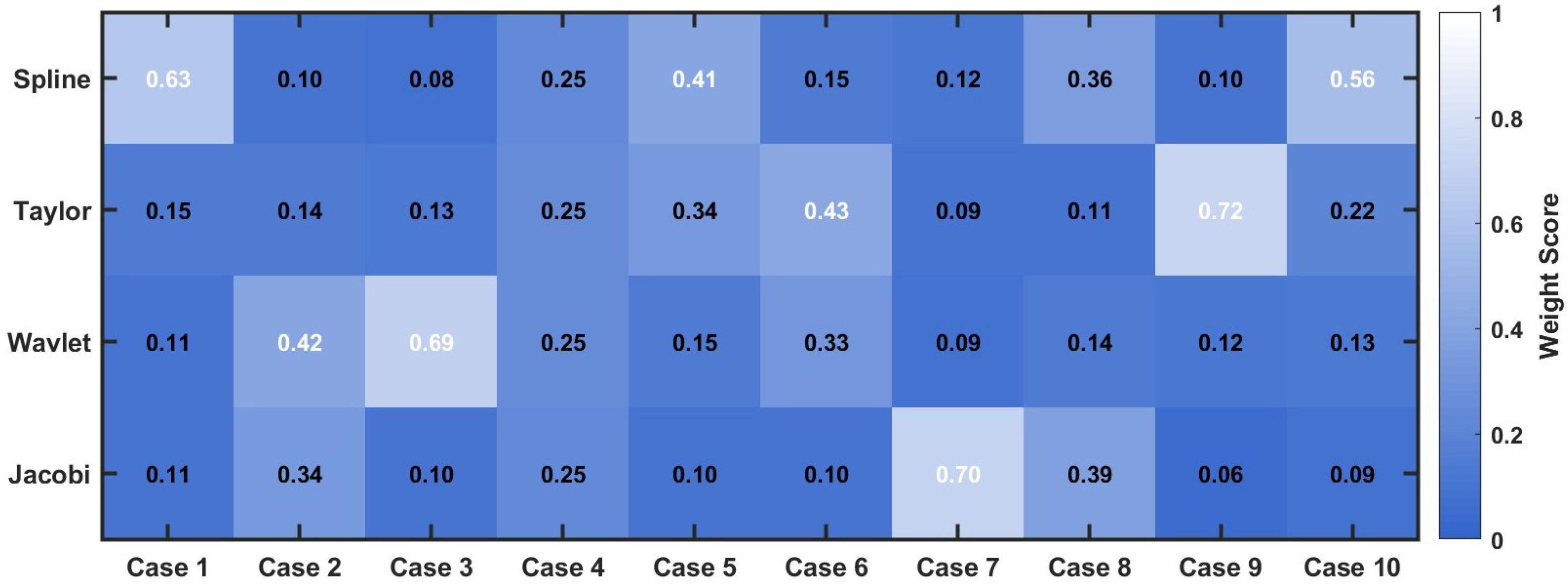
This study systematically validates the effectiveness and superiority of the multi-expert adaptive prediction framework through visual analysis of ten time-series load forecasting cases. As shown in Figure 7, the visualization results based on the NSG2020 dataset clearly demonstrate the significant advantages of the multi-expert adaptive mechanism in complex time-series prediction tasks. The visual analysis reveals that the multi-expert adaptive prediction model can intelligently adjust the contribution weights of different experts according to the inherent characteristics of input sequences. Across various prediction scenarios, the model automatically identifies the most suitable combination of experts, demonstrating strong environmental adaptability. This dynamic weight allocation mechanism ensures that the model maintains optimal prediction performance when confronted with diverse load patterns. The experimental results fully demonstrate that the multi-expert collaborative framework surpasses the performance limitations of single-expert models, achieving significant improvements in prediction accuracy through complementary advantages among experts. This framework not only possesses the capability to handle complex temporal patterns but also exhibits excellent generalization performance and robustness, providing a more reliable and effective solution for time-series load forecasting tasks.
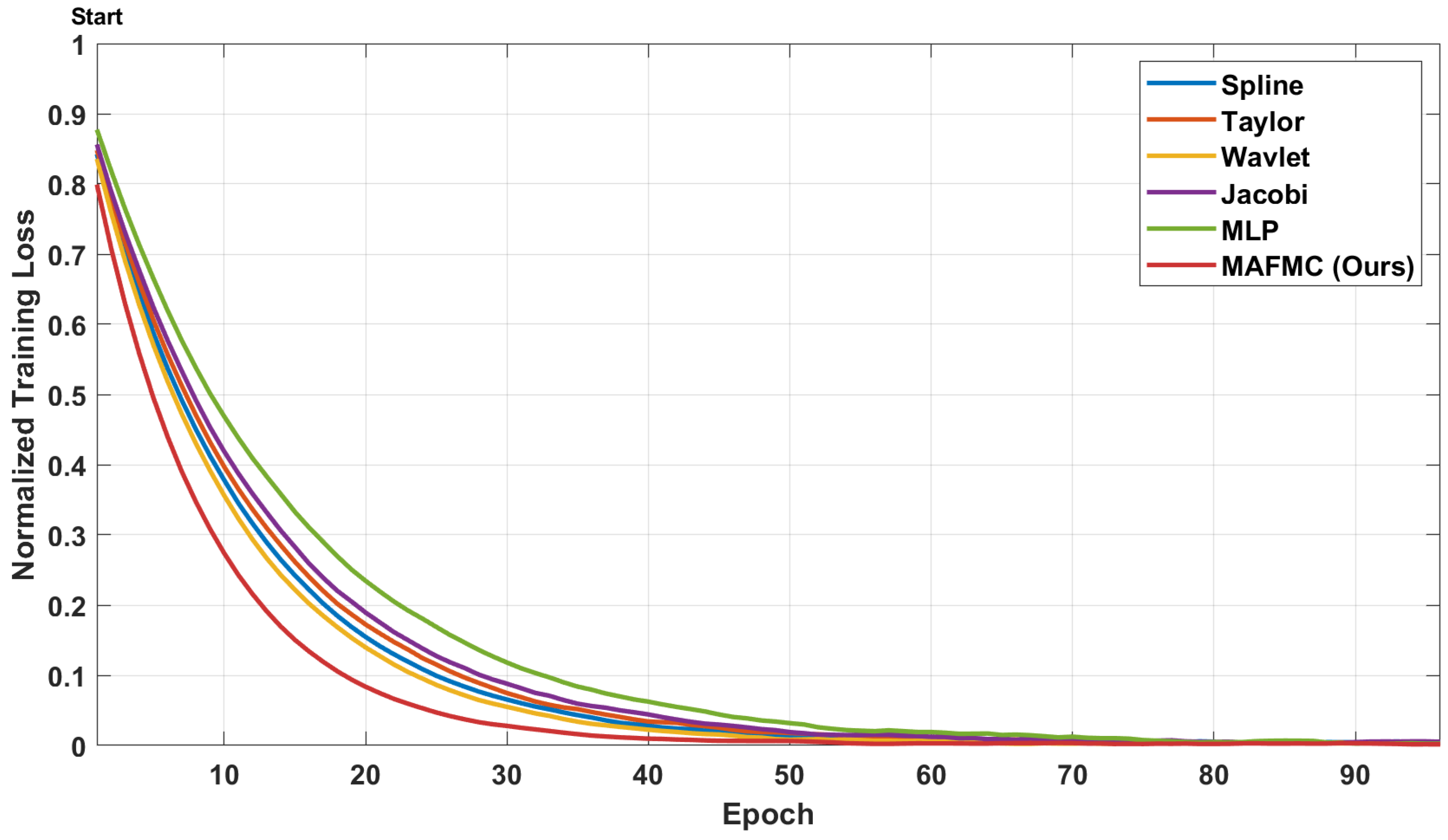
Meanwhile, this study provides a comparative analysis of the training loss convergence behaviors between single-expert models and the multi-expert mixture model on the NSG2020 dataset, thoroughly validating the effectiveness of the multi-expert collaboration mechanism. As illustrated in Figure 8, the multi-expert mixture model demonstrates significant performance advantages, exhibiting not only faster convergence speed but also achieving substantially lower stabilized loss values compared to any individual expert model. Experimental results reveal that while individual expert models—including Spline, Taylor, Wavlet, Jacobi, and MLP—demonstrate specialized advantages in recognizing specific data patterns, they all exhibit limitations when confronted with the complex heterogeneity of power load data. In contrast, the multi-expert collaboration mechanism within the MAFMC framework, facilitated by a dynamic gating network, enables intelligent weight allocation among experts, automatically selecting the most suitable expert combinations based on the specific characteristics of input sequences. This adaptive fusion strategy allows the model to fully leverage the complementary strengths of different experts, demonstrating enhanced adaptability and robustness when processing load data with diverse statistical properties and fluctuation patterns. These findings provide compelling evidence for the application of multi-expert collaboration in complex time-series forecasting tasks, further confirming the theoretical advantages of the MAFMC framework in handling the heterogeneity and non-linear dynamics inherent in power load data.

5. Discussion

The empirical results presented herein compellingly demonstrate the superiority of the MAFMC framework, which consistently outperformed six leading baselines across three diverse datasets. This section discusses the theoretical contributions and practical significance of our findings, contextualizes them within the broader field, and acknowledges the limitations and implementation barriers that pave the way for future research.
At the heart of MAFMC’s success lies the novel integration of a mixture-of-experts (MoE) architecture with Kolmogorov–Arnold Network (KAN) predictors. This design marks a significant departure from conventional deep learning models that typically rely on a monolithic, single-predictor head. As revealed by the ablation study (MAFMC w/o MOE), removing this component leads to a substantial drop in performance. The theoretical strength of this approach is its ability to model the heterogeneous nature of power load data, where different underlying patterns (e.g., seasonal trends, weekday/weekend cycles, and stochastic fluctuations) co-exist. Instead of forcing a single model to learn a generalized, and therefore compromised, representation, the MoE-KAN architecture allows for the concurrent learning of specialized sub-models. Each KAN expert, with its distinct basis functions, can become adept at capturing specific temporal dynamics, and the gating network learns to dynamically allocate resources based on the input’s characteristics. This enhances the model’s capacity to fit complex, non-linear distributions inherent in modern, renewable-dominated power grids.
Beyond its predictive accuracy, the framework’s iterative auto-regressive learning mechanism represents a critical contribution to the practical deployment of forecasting models. Traditional methods are often constrained by a fixed prediction horizon, a significant operational bottleneck that requires costly retraining or the maintenance of multiple models for different forecasting needs. Our iterative approach, whose importance was validated by the performance degradation in the MAFMC w/o IAL variant, endows the model with unparalleled flexibility. By decomposing long-range forecasting into a sequence of single-patch predictions, MAFMC can generate forecasts of arbitrary length on-demand. This enhances the utility of the model in dynamic operational environments where forecasting requirements can change rapidly due to market conditions or unexpected events, thereby providing grid operators with greater agility.
It is also noteworthy that MAFMC not only surpassed domain-specific baselines but also outperformed state-of-the-art general time-series forecasting models like TimeCMA and TimeKAN. This finding is significant as it underscores the efficacy of our domain-aware architectural design. While general-purpose architectures provide a powerful foundation, their thoughtful adaptation and integration with specialized components—such as the multi-scale patchization strategy to handle noise and the iterative mechanism for flexibility—can unlock new levels of performance on complex, real-world tasks like power load forecasting. This suggests a promising research direction where powerful foundational models are tailored to specific problem domains.
While this study establishes a new benchmark in power load forecasting, a candid discussion of its limitations and potential barriers to real-world implementation is warranted. The current model relies solely on historical load data; a key direction for future work is integrating exogenous variables such as dynamic electricity prices and demand response signals to enable more economically aware predictions. However, the availability and quality of such diverse data streams represent a significant practical barrier, often requiring complex data engineering to synchronize disparate sources. Second, the computational resources required for training a sophisticated model like MAFMC are non-trivial. While the performance gains are substantial, deploying and periodically retraining such models may pose a challenge for utilities with limited GPU infrastructure. Third, integration with existing forecasting tools and legacy energy management systems (EMS) presents another hurdle. Transitioning from a research prototype to an operational tool requires robust APIs, fault tolerance, and ensuring the model’s outputs are interpretable to grid operators who must trust its predictions for critical decision-making. Addressing these practical barriers—alongside scientific extensions such as exploring data confidentiality via federated learning—does not diminish the core contributions of this work. Instead, it provides a comprehensive roadmap for evolving MAFMC from a high-performing algorithm into a robust, deployable, and secure decision-support tool for the next generation of intelligent grids.

6. Conclusions

This study successfully introduced the multi-scale adaptive power load forecasting with multi-expert collaboration framework, effectively overcoming two critical limitations in deep learning-based forecasting: the rigidity of fixed-length prediction horizons and the insufficient capacity of conventional architectures to capture heterogeneous temporal patterns. By innovatively integrating a mixture-of-experts architecture featuring diverse KAN predictors with an iterative auto-regressive learning strategy, MAFMC achieved state-of-the-art performance across three real-world datasets, demonstrating substantial reductions in MSE and MAE compared to six leading baselines. The novel MoE-KAN prediction module exhibited superior adaptability to complex, non-linear load dynamics, while the iterative residual mechanism enabled highly flexible, variable-length forecasting without laborious retraining, significantly enhancing operational flexibility for sustainable grid management. Building upon this robust foundation, future work will focus on enhancing the model’s practical utility by incorporating key operational factors such as dynamic electricity prices, demand response signals, and energy storage status to create more economically aware predictions. Furthermore, to address the critical issue of data confidentiality, we will explore the integration of privacy-preserving mechanisms like federated learning. Finally, the framework’s modular design provides a clear pathway for expansion into more complex multi-energy system scenarios, such as combined cooling, heating, and power applications, ultimately evolving MAFMC into a comprehensive and secure decision-support tool for next-generation intelligent grids.

Author Contributions

Conceptualization, Z.C.; Methodology, Z.T., W.D., M.L. and Z.C.; Validation, W.D.; Investigation, L.L.; Resources, L.L.; Data curation, L.L.; Writing—original draft, Z.T. and M.L.; Writing—review & editing, Z.T. and M.L.; Visualization, W.D. and Z.C.; Supervision, W.D., L.L. and Z.C.; Funding acquisition, Zhikui Chen. All authors have read and agreed to the published version of the manuscript.

Funding

This research received no external funding.

Institutional Review Board Statement

Not applicable.

Informed Consent Statement

Not applicable.

Data Availability Statement

Data are contained within the article.

Conflicts of Interest

Author Zengyao Tian, Wenchen Deng and Li Lv were employed by the company Shenyang Institute of Computing Technology. The remaining authors declare that the research was conducted in the absence of any commercial or financial relationships that could be construed as a potential conflict of interest.

References

  1. Pentsos, V.; Tragoudas, S.; Wibbenmeyer, J.; Khdeer, N. A hybrid LSTM-Transformer model for power load forecasting. IEEE Trans. Smart Grid 2025, 16, 2624–2634. [Google Scholar] [CrossRef]
  2. Jalalifar, R.; Delavar, M.R.; Ghaderi, S.F. A novel approach for photovoltaic plant site selection in megacities utilizing power load forecasting and fuzzy inference system. Renew. Energy 2025, 243, 122527. [Google Scholar] [CrossRef]
  3. Peng, X.; Yang, X. Short-and medium-term power load forecasting model based on a hybrid attention mechanism in the time and frequency domains. Expert Syst. Appl. 2025, 278, 127329. [Google Scholar] [CrossRef]
  4. Gao, J.; Liu, M.; Li, P.; Zhang, J.; Chen, Z. Deep Multiview Adaptive Clustering With Semantic Invariance. IEEE Trans. Neural Netw. Learn. Syst. 2024, 35, 12965–12978. [Google Scholar] [CrossRef]
  5. Gao, J.; Liu, M.; Li, P.; Laghari, A.A.; Javed, A.R.; Victor, N.; Gadekallu, T.R. Deep incomplete multiview clustering via information bottleneck for pattern mining of data in extreme-environment IoT. IEEE Internet Things J. 2024, 11, 26700–26712. [Google Scholar] [CrossRef]
  6. Fan, G.-F.; Han, Y.-Y.; Li, J.-W.; Peng, L.-L.; Yeh, Y.-H.; Hong, W.-C. A hybrid model for deep learning short-term power load forecasting based on feature extraction statistics techniques. Expert Syst. Appl. 2024, 238, 122012. [Google Scholar] [CrossRef]
  7. Jalalifar, R.; Delavar, M.R.; Ghaderi, S.F. SAC-ConvLSTM: A novel spatio-temporal deep learning-based approach for a short term power load forecasting. Expert Syst. Appl. 2024, 237, 121487. [Google Scholar] [CrossRef]
  8. Yang, F.; Fu, X.; Yang, Q.; Chu, Z. Decomposition strategy and attention-based long short-term memory network for multi-step ultra-short-term agricultural power load forecasting. Expert Syst. Appl. 2024, 238, 122226. [Google Scholar] [CrossRef]
  9. Mao, Q.; Wang, L.; Long, Y.; Han, L.; Wang, Z.; Chen, K. A blockchain-based framework for federated learning with privacy preservation in power load forecasting. Knowl.-Based Syst. 2024, 284, 111338. [Google Scholar] [CrossRef]
  10. Dong, J.; Luo, L.; Lu, Y.; Zhang, Q. A parallel short-term power load forecasting method considering high-level elastic loads. IEEE Trans. Instrum. Meas. 2023, 72, 1–10. [Google Scholar] [CrossRef]
  11. Nahid, J.; Ongsakul, W.; Singh, J.G.; Roy, J. Short-term customer-centric electric load forecasting for low carbon microgrids using a hybrid model. Energy Syst. 2024. [Google Scholar] [CrossRef]
  12. Wang, Y.; Hao, Y.; Zhao, K.; Yao, Y. Stochastic configuration networks for short-term power load forecasting. Inf. Sci. 2025, 689, 121489. [Google Scholar] [CrossRef]
  13. Guo, W.; Liu, S.; Weng, L.; Liang, X. Power grid load forecasting using a CNN-LSTM network based on a multi-modal attention mechanism. Appl. Sci. 2025, 15, 2435. [Google Scholar] [CrossRef]
  14. Zhu, L.; Gao, J.; Zhu, C.; Deng, F. Short-term power load forecasting based on spatial-temporal dynamic graph and multi-scale Transformer. J. Comput. Des. Eng. 2025, 12, 92–111. [Google Scholar] [CrossRef]
  15. Hu, X.; Li, H.; Si, C. Improved composite model using metaheuristic optimization algorithm for short-term power load forecasting. Electr. Power Syst. Res. 2025, 241, 111330. [Google Scholar] [CrossRef]
  16. Somvanshi, S.; Javed, S.A.; Islam, M.M.; Pandit, D.; Das, S. A survey on Kolmogorov-Arnold network. ACM Comput. Surv. 2025, 58, 55. [Google Scholar] [CrossRef]
  17. Gbadega, P.A.; Sun, Y. Enhancing medium-term electric load forecasting accuracy leveraging swarm intelligence and neural networks optimization. In Proceedings of the 2024 18th International Conference on Probabilistic Methods Applied to Power Systems (PMAPS), Auckland, New Zealand, 24–26 June 2024; pp. 1–6. [Google Scholar]
  18. Lv, Z.; Wang, L.; Guan, Z.; Wu, J.; Du, X.; Zhao, H.; Guizani, M. An optimizing and differentially private clustering algorithm for mixed data in SDN-based smart grid. IEEE Access 2019, 7, 45773–45782. [Google Scholar] [CrossRef]
  19. Tsai, J.-L.; Lo, N.-W. Secure anonymous key distribution scheme for smart grid. IEEE Trans. Smart Grid 2015, 7, 906–914. [Google Scholar] [CrossRef]
  20. Chalmers, C.; Fergus, P.; Montanez, C.A.C.; Sikdar, S.; Ball, F.; Kendall, B. Detecting activities of daily living and routine behaviours in dementia patients living alone using smart meter load disaggregation. IEEE Trans. Emerg. Top. Comput. 2020, 10, 157–169. [Google Scholar] [CrossRef]
  21. Weber, M.; Turowski, M.; Çakmak, H.K.; Mikut, R.; Kühnapfel, U.; Hagenmeyer, V. Data-driven copy-paste imputation for energy time series. IEEE Trans. Smart Grid 2021, 12, 5409–5419. [Google Scholar] [CrossRef]
  22. Ullah, A.; Javaid, N.; Javed, M.U.; Pamir; Kim, B.-S.; Bahaj, S.A. Adaptive data balancing method using stacking ensemble model and its application to non-technical loss detection in smart grids. IEEE Access 2022, 10, 133244–133255. [Google Scholar] [CrossRef]
  23. Li, K.; Huang, W.; Hu, G.; Li, J. Ultra-short term power load forecasting based on CEEMDAN-SE and LSTM neural network. Energy Build. 2023, 279, 112666. [Google Scholar] [CrossRef]
  24. Zhang, S.; Chen, R.; Cao, J.; Tan, J. A CNN and LSTM-based multi-task learning architecture for short and medium-term electricity load forecasting. Electr. Power Syst. Res. 2023, 222, 109507. [Google Scholar] [CrossRef]
  25. Hua, H.; Liu, M.; Li, Y.; Deng, S.; Wang, Q. An ensemble framework for short-term load forecasting based on parallel CNN and GRU with improved ResNet. Electr. Power Syst. Res. 2023, 216, 109057. [Google Scholar] [CrossRef]
  26. Gong, J.; Qu, Z.; Zhu, Z.; Xu, H.; Yang, Q. Ensemble models of TCN-LSTM-LightGBM based on ensemble learning methods for short-term electrical load forecasting. Energy 2025, 318, 134757. [Google Scholar] [CrossRef]
  27. Ma, W.; Wu, W.; Ahmed, S.F.; Liu, G. Techno-economic feasibility of utilizing electrical load forecasting in microgrid optimization planning. Sustain. Energy Technol. Assess. 2025, 73, 104135. [Google Scholar] [CrossRef]
  28. Liu, M.; Xia, C.; Xia, Y.; Deng, S.; Wang, Y. TDCN: A novel temporal depthwise convolutional network for short-term load forecasting. Int. J. Electr. Power Energy Syst. 2025, 165, 110512. [Google Scholar] [CrossRef]
  29. Sidharth, S.S.; Keerthana, A.R.; Gokul, R.; Anas, K.P. Chebyshev polynomial-based Kolmogorov-Arnold networks: An efficient architecture for nonlinear function approximation. arXiv 2024, arXiv:2405.07200. [Google Scholar]
  30. Li, Z. Kolmogorov-Arnold networks are radial basis function networks. arXiv 2024, arXiv:2405.06721. [Google Scholar] [CrossRef]
  31. Abd Elaziz, M.; Fares, I.A.; Aseeri, A.O. CKAN: Convolutional Kolmogorov–Arnold networks model for intrusion detection in IoT environment. IEEE Access 2024, 12, 134837–134851. [Google Scholar] [CrossRef]
  32. Li, C.; Liu, X.; Li, W.; Wang, C.; Liu, H.; Liu, Y.; Chen, Z.; Yuan, Y. U-KAN makes strong backbone for medical image segmentation and generation. In Proceedings of the Thirty-Ninth AAAI Conference on Artificial Intelligence (AAAI’25), Philadelphia, PA, USA, 25 February–4 March 2025; pp. 4652–4660. [Google Scholar]
  33. Shukla, K.; Toscano, J.D.; Wang, Z.; Zou, Z.; Karniadakis, G.E. A comprehensive and fair comparison between MLP and KAN representations for differential equations and operator networks. Comput. Methods Appl. Mech. Eng. 2024, 431, 117290. [Google Scholar] [CrossRef]
  34. Wang, Y.; Sun, J.; Bai, J.; Anitescu, C.; Eshaghi, M.S.; Zhuang, X.; Rabczuk, T.; Liu, Y. Kolmogorov Arnold Informed neural network: A physics-informed deep learning framework for solving forward and inverse problems based on Kolmogorov Arnold Networks. arXiv 2024, arXiv:2406.11045. [Google Scholar] [CrossRef]
  35. Liu, C.; Xu, Q.; Miao, H.; Yang, S.; Zhang, L.; Long, C.; Li, Z.; Zhao, R. TimeCMA: Towards llm-empowered multivariate time series forecasting via cross-modality alignment. In Proceedings of the Thirty-Ninth AAAI Conference on Artificial Intelligence (AAAI’25), Philadelphia, PA, USA, 25 February–4 March 2025; pp. 18780–18788. [Google Scholar]
  36. Huang, S.; Zhao, Z.; Li, C.; Bai, L. TimeKAN: KAN-based Frequency Decomposition Learning Architecture for Long-term Time Series Forecasting. arXiv 2025, arXiv:2502.06910. [Google Scholar] [CrossRef]
  37. Zhou, H.; Zhang, S.; Peng, J.; Zhang, S.; Li, J.; Xiong, H.; Zhang, W. Informer: Beyond Efficient Transformer for Long Sequence Time-Series Forecasting. In Proceedings of the Thirty-Fifth AAAI Conference on Artificial Intelligence (AAAI 2021), Virtually, 2–9 February 2021; pp. 11106–11115. [Google Scholar]
  38. Zhou, T.; Ma, Z.; Wen, Q.; Wang, X.; Sun, L.; Jin, R. FEDformer: Frequency Enhanced Decomposed Transformer for Long-term Series Forecasting. In Proceedings of the 39th International Conference on Machine Learning (ICML), Baltimore, MD, USA, 17–23 July 2022; pp. 27268–27286. [Google Scholar]
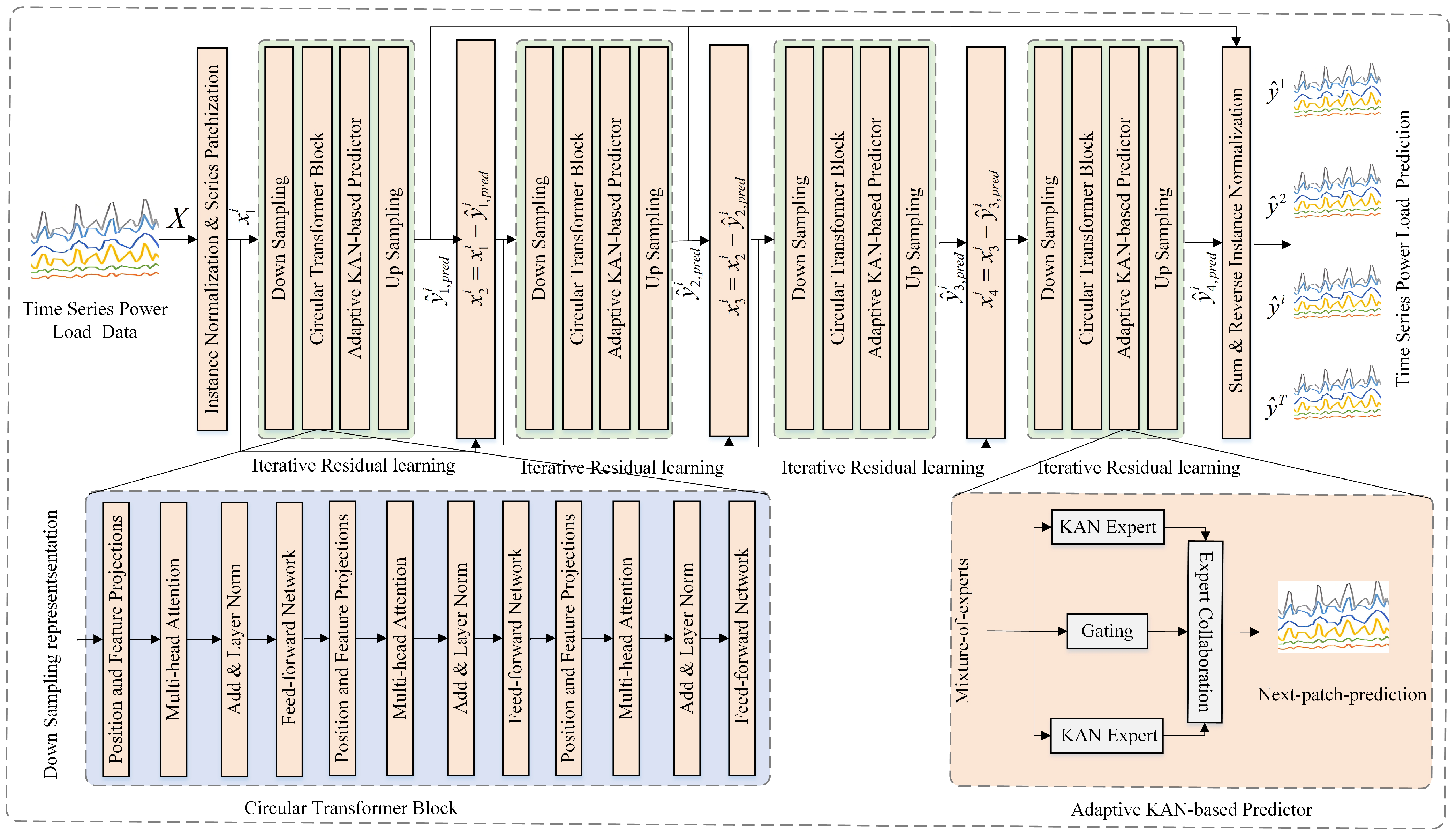
Figure 1. The overall architecture of MAFMC.
Sustainability 17 10434 g001
Figure 2. The Nemenyi test on the three datasets. The red circle marks the model with the best overall performance (lowest average rank) in the Nemenyi statistical test.
Sustainability 17 10434 g002
Figure 3. Ablation study on the NSG-2020 dataset. FPL denotes the future prediction length.
Sustainability 17 10434 g003
Figure 4. The parameter analysis on the NSG2020 dataset. FPL denotes the future prediction length. (a) The learning rate (LR). (b) The patch sizes. (c) Number of experts (M).
Sustainability 17 10434 g004aSustainability 17 10434 g004b
Figure 5. Input length study on the NSG2020 dataset.
Sustainability 17 10434 g005
Figure 6. Convergence analysis on the three dataset. (a) Training loss convergence. (b) Validation loss convergence.
Sustainability 17 10434 g006
Figure 7. Visualization of the multi-expert adaptive prediction on the NSG2020 dataset.
Sustainability 17 10434 g007
Figure 8. The training loss of the single/mixture prediction on the NSG2020 dataset.
Sustainability 17 10434 g008
Table 1. The statistical summarization of three datasets.
NameVariablesFrequencyLengthTrain/Valid/Test
Electricity3211 h26,30460%/10%/30%
NSG-2020515 min35,13660%/10%/30%
NSG-2023515 min35,13660%/10%/30%
Table 2. Power load forecasting results with six methods. Input length = 336 for all methods. FPL denotes the future prediction length. Bold indicates the best results.
DatasetFPLMAFMCTimeCMATimeKANHybrid-LTLDTformerConvLSTMMTMVInformerFEDformer
MSE MAE MSE MAE MSE MAE MSE MAE MSE MAE MSE MAE MSE MAE MAE MSE MAE MSE
NSG2020480.0140.0420.0150.0450.0170.0480.0190.0510.0200.0520.0220.0540.0250.0570.0210.0500.0190.049
960.0280.1190.0320.1250.0350.1290.0380.1340.0400.1370.0420.1400.0450.1450.0390.1380.0370.135
1920.0450.1540.0520.1620.0580.1680.0640.1740.0670.1770.0700.1800.0750.1850.0650.1690.0660.167
3360.0640.1860.0880.1980.0950.2050.1030.2120.1080.2170.1140.2220.1210.2270.1090.2120.1050.197
7200.1170.2550.1340.2680.1450.2750.1560.2850.1620.2900.1690.2950.1780.3030.1620.2800.1580.284
Avg0.0530.1510.0640.1610.0710.1690.0790.1770.0830.1810.0880.1860.0970.1940.0790.1690.0770.164
NSG2023480.0120.0970.0130.1020.0140.1050.0160.1100.0180.1150.0200.1200.0220.1250.0190.1170.0190.118
960.0490.1520.0530.1600.0580.1650.0630.1700.0680.1750.0730.1800.0780.1850.0700.1750.0690.173
1920.0820.2020.0880.2100.0950.2150.1030.2200.1110.2250.1190.2300.1270.2350.1160.2240.1120.222
3360.1260.2570.1350.2650.1450.2700.1560.2750.1680.2800.1800.2850.1930.2900.1730.2770.1750.278
7200.2740.3870.2950.4000.3170.4100.3410.4200.3660.4300.3920.4400.4200.4500.3720.4210.3660.414
Avg0.1090.2190.1170.2270.1260.2330.1360.2390.1460.2450.1570.2510.1680.2570.1500.2420.1480.241
Electricity480.1220.2230.1300.2300.1380.2370.1450.2440.1550.2500.1650.2570.1750.2630.1620.2520.1630.253
960.1550.2370.1650.2450.1740.2660.1850.2610.1950.2690.2050.2770.2150.2850.2000.2720.1980.267
1920.1620.2540.1730.2630.1820.2720.1950.2810.2070.2900.2190.2990.2310.3080.2140.2930.2080.288
3360.1870.2740.1980.2830.1970.2860.2230.3010.2370.3100.2520.3190.2680.3280.2470.3100.2420.308
7200.2250.3190.2380.3280.2360.3200.2670.3460.2840.3550.3020.3640.3210.3730.3000.3600.2930.357
Avg0.1700.2610.1800.2700.1850.2580.1830.2860.2150.2940.2280.2950.2350.3100.2240.2970.2200.294
Table 3. All models are trained exclusively on the Electricity dataset and subsequently tested on the NSG-2020 dataset. Input length = 336 for all methods. FPL denotes the future prediction length. Bold indicates the best results.
DatasetFPLMAFMCTimeCMATimeKANHybrid-LTLDTformer
MSE MAE MSE MAE MSE MAE MSE MAE MSE MAE
NSG2020480.0220.0580.0260.0670.0290.0720.0340.0750.0480.082
960.0390.1330.0470.1450.0520.1490.0550.1620.0620.177
1920.0570.1710.0680.1870.0720.1920.0750.2000.0820.217
3360.0770.1980.0970.2130.0990.2150.1130.2270.1280.227
7200.1280.2810.1470.2920.1510.2950.1760.3050.1820.313
Disclaimer/Publisher’s Note: The statements, opinions and data contained in all publications are solely those of the individual author(s) and contributor(s) and not of MDPI and/or the editor(s). MDPI and/or the editor(s) disclaim responsibility for any injury to people or property resulting from any ideas, methods, instructions or products referred to in the content.