Article

A Universal Urban Flood Risk Model Based on Particle-Swarm-Optimization-Enhanced Spiking Graph Convolutional Networks

1
School of Computer Science and Technology, Dongguan University of Technology, Dongguan 523808, China
2
School of Environment and Civil Engineering, Dongguan University of Technology, Dongguan 523808, China
3
Guangdong Provincial Key Laboratory of Intelligent Disaster Prevention and Emergency Technologies for Urban Lifeline Engineering, Dongguan 523808, China
*
Authors to whom correspondence should be addressed.
Sustainability 2025, 17(22), 9973; https://doi.org/10.3390/su17229973 (registering DOI)
Submission received: 3 September 2025 / Revised: 4 November 2025 / Accepted: 4 November 2025 / Published: 7 November 2025
(This article belongs to the Section Hazards and Sustainability)

Abstract

As climate change and urbanization accelerate, urban flooding poses an increasingly severe threat to urban residents and their properties, creating an urgent need for effective solutions to achieve sustainable urban disaster management. While physically based hydrodynamic models can accurately simulate urban floods, they are data- and computational-resource-demanding. Meanwhile, artificial intelligence models driven by data often lack generalizability across different urban areas. To address these challenges, integrating spiking neural networks, graph convolutional networks (GCNs), and particle swarm optimization (PSO), a novel PSO-enhanced spiking graph convolutional neural network (P-SGCN) is proposed. The model is trained on a self-constructed dataset based on social media data, incorporating six representative Chinese cities: Beijing, Shanghai, Shenzhen, Wuhan, Hangzhou, and Shijiazhuang. These cities were selected for their diverse urban and flood characteristics to enhance model generalizability. The P-SGCN significantly outperforms baseline models such as GCN and long short-term memory, achieving an accuracy, precision, recall, and F1 score of 0.846, 0.847, 0.846, and 0.846, respectively. These results indicate our model’s capability to effectively handle data from six cities while maintaining high accuracy. Meanwhile, the model improves single-city performance through transfer learning and offers extremely fast inference with minimal energy consumption, making it suitable for real-time applications. This study provides a scalable and generalizable solution for urban flood risk management, with potential applications in disaster preparedness and urban planning across varied geographic and socioeconomic contexts.

1. Introduction

Urban flooding is an emerging threat to human life and property worldwide. Climate change and urbanization have intensified urban flooding risks [1,2,3,4]. Floods account for more than 30% of total disaster losses annually [5]. Specifically, the 21 July 2012 flood in Beijing, China, resulted in over 70 deaths and affected 1.6 million people [6]; the flood in Zhengzhou, China, on 20 July 2021, led to hundreds of deaths and economic losses of RMB 40 billion [7]. Similar catastrophic events include the Mila floods in Algeria and the May 2010 floods in the Lower Kelani River Basin, Colombo, Sri Lanka, both of which caused severe human and economic losses [8]. These incidents underscore the urgent need for effective urban flood management and adaptation strategies in response to the challenges posed by climate change and urbanization [9]. Therefore, a reliable and rapid urban flood risk assessment model is vital for reducing the risk of disasters, and it also helps with urban planning and disaster management [2,10,11]. Urban flood risk assessment models employ a multifaceted approach to potential analysis of flood risks, which considers a range of factors, including topographic elevation, meteorological data and drainage system capacity, among others [12,13]. These factors are combined with simulation algorithms to generate the water depth, area affected and disaster level of a specific area [14]. In recent years, a variety of models have been developed and applied, broadly classified into physically based and data-driven models [15].
Physically based models simulate flood sequences by numerically solving hydrodynamic equations, ranging from simple one-dimensional to intricate three-dimensional structures [4,16]. Models such as the soil and water assessment tool [17], the system hydrologique européen [18], the storm water management model [19], and high-power impulse magnetron sputtering [20] depend on extensive datasets, including initial and boundary conditions, spatial data from digital elevation models (DEMs) [21], land use patterns, and hydrometeorological information such as rainfall and river flow rates [22]. These models are adept at representing detailed flood dynamics and providing accurate predictions of flood impacts [18]. To better interpret and utilize flood model outputs, multi-criteria decision analysis (MCDA) models [23] are often applied—such as prioritizing risk zones or selecting mitigation measures. Common MCDA methods include the analytic hierarchy process, the best–worst method, and the technique for order preference by similarity to the ideal solution, which integrate multiple indicators for scientific decision-making [24]. However, these data, especially high-resolution data, are sometimes difficult to access or unavailable. Furthermore, these models require measured flood information for calibration and validation, which is challenging to collect, particularly during flood events [25]. Without high-quality input and validation data, the simulation accuracy and transferability of these models are questionable.
In contrast, data-driven models use statistical or artificial intelligence (AI) methods to identify risk factors and predict potential flood scenarios, providing a swift and versatile approach to urban flood risk assessment [26,27]. These AI models focus on the relationships between input variables (contributing factors, such as precipitation, elevation, building density, river networks, road networks, etc.) and output measures (including the extent or severity of urban flooding) [25]. Unlike physically based models, they do not require complex, high-resolution urban data and can provide accurate and efficient results by considering key factors such as average elevation, population density, and building density [28]. However, collecting data on key factors, such as urban flood water depth, remains a significant challenge. Additionally, existing AI models are typically focused on specific cities or even small areas within them [27,29], which may limit their applicability in data-scarce regions.
To overcome urban flood data scarcity, this study constructs a mixed-city flood risk dataset encompassing six Chinese cities, integrating flood event reports (time, location, severity) from Sina Weibo and independently sourced precipitation, building, and population data. While social media enables rapid, crowdsourced flood monitoring [25,30,31], its inherent volatility and potential inaccuracies (e.g., misreported locations or non-flood-related posts) often hinder reliability [31,32]. To mitigate these issues, this study implements a rigorous validation protocol, cross-verifying social-media-derived flood records against official municipal flood logs to ensure spatiotemporal accuracy.
To address the limitations of existing urban flood risk models, particularly their narrow applicability to single cities and reliance on localized training data, this study pioneeringly introduces the particle-swarm-optimization-enhanced spiking graph convolutional neural network (P-SGCN), a universal flood risk assessment model that integrates graph convolutional network (GCN) [33,34], spiking neural network (SNN) [35], and particle swarm optimization (PSO) [36]. GCN excels at modeling spatial dependencies in urban systems, such as elevation gradients and building distributions, enabling cross-city generalization by capturing shared topological patterns [37]. In this study, GCNs are first employed to extract spatial relationships between urban nodes, providing a foundation for subsequent temporal analysis. SNNs, inspired by the human brain’s spike-based information processing, are adept at handling temporal data and exhibit significantly lower energy consumption compared to traditional recurrent neural networks [38]. In this study, SNNs process time-series data that integrate rainfall information and spatial features extracted by GCNs to model flood dynamics. PSO, a swarm intelligence algorithm, is widely recognized for its effectiveness in optimizing neural network architectures and hyperparameters [39]. Beyond this application, it has also been successfully utilized to solve other optimization problems, such as finding parameters of equations of state [40]. In this study, PSO is employed to systematically optimize our spiking graph convolutional network (SGCN) model, ensuring robust performance across diverse urban environments.
In the experimental phase, P-SGCN is applied to our mixed-city dataset. The results are compared with two machine learning models, GCN and long short-term memory (LSTM), which are well-known for extracting patterns from sequential data and are widely used for hydrological modeling [41,42]. Both visual and statistical comparisons show that P-SGCN outperforms baseline models, showcasing its universal applicability across diverse urban environments. Transfer learning [43] further validates its universality: fine-tuning the pre-trained P-SGCN model with single-city data achieves up to a 12.4% accuracy improvement. This pre-training capability positions P-SGCN as a foundational platform for global scalability, enabling seamless adaptation to worldwide flood data through transfer learning.
In conclusion, the main goal of this study is to develop a scalable and universal urban flood risk assessment model. This model is expected to provide a practical solution for urban flood risk assessment, with significant potential for supporting disaster preparedness and urban planning across diverse geographic and socioeconomic contexts.

2. Materials and Methods

2.1. Study Area

This study aims to develop a universal urban flood model with global applicability. China was chosen as the initial focus due to its unique combination of geographic and climatic diversity, rapid urban development, and significant flood challenges [44]. Additionally, China’s large population, high internet penetration, and advanced digital infrastructure enable the collection of urban flood-related data from social media [45,46]. These factors make it an ideal testing ground to overcome the limitations of existing models and develop solutions adaptable to diverse urban environments. Figure 1 shows some samples of urban floods in China.
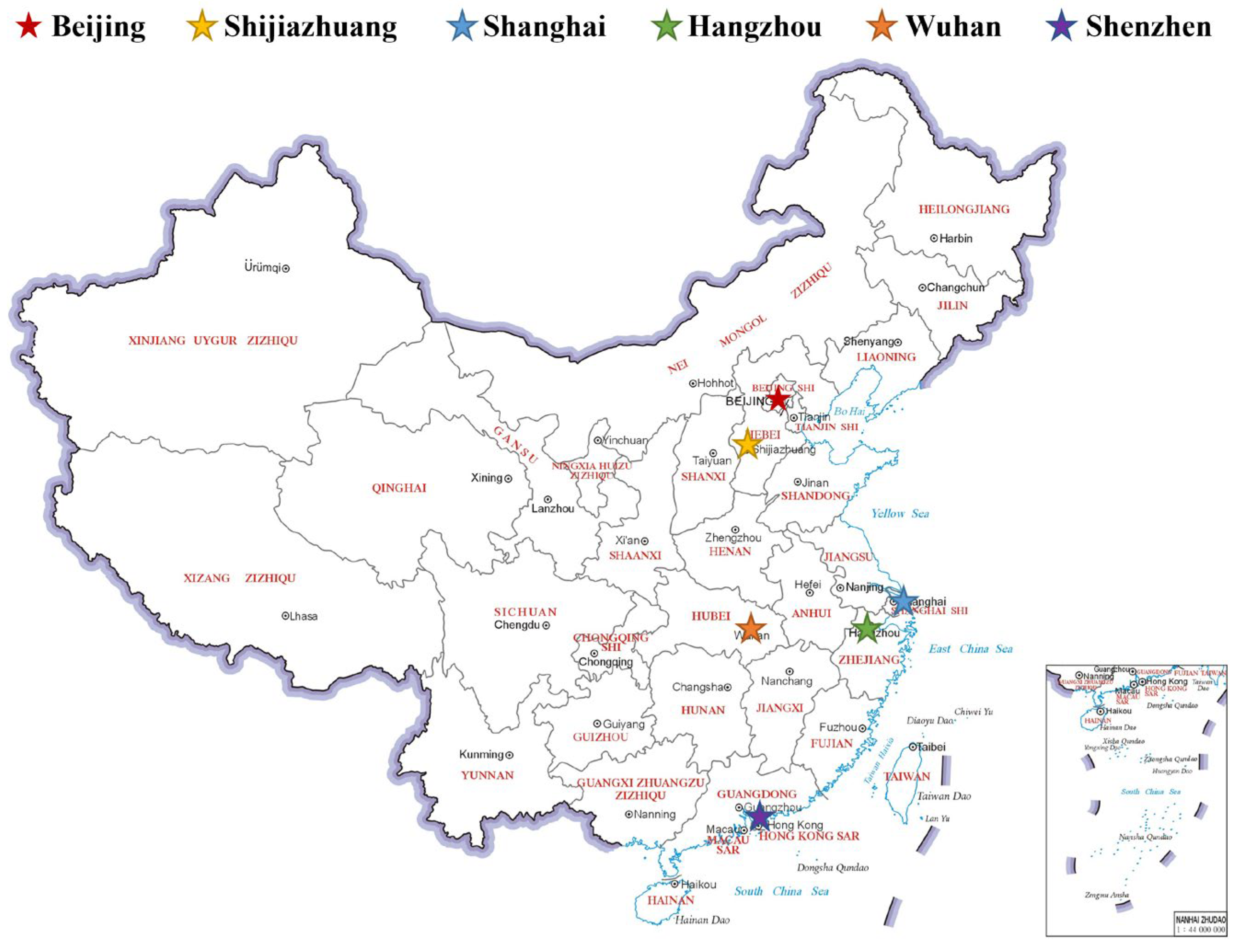
China’s cities exhibit a wide range of flood-prone conditions, particularly in the eastern regions, where flooding risks are heightened due to dense populations and intensive urbanization [47,48,49]. To capture this diversity, six representative cities, Beijing, Shanghai, Shenzhen, Hangzhou, Wuhan, and Shijiazhuang, were selected, as shown in Figure 2. These cities were chosen for their distinct geographic distribution (covering northern, eastern, and central China), population density (from megacities to large cities), and economic development stages (from highly developed metropolises to rapidly developing industrial hubs); this ensures the model is trained on a dataset reflecting diverse urban characteristics and flood risk backgrounds (e.g., coastal flooding in Shanghai vs. inland rainfall flooding in Wuhan).
Focusing on Chinese cities provides a scalable framework for broader application. By using China as a representative case of global urban flooding challenges, this study develops localized insights that can inform universal flood risk management strategies, establishing a foundation for extending the model to diverse regions worldwide.

2.2. Mixed-City Flood Risk Dataset

The lack of publicly available urban flood datasets poses a significant challenge to developing generalized flood risk models. To overcome this, this study constructed a mixed-city flood risk dataset using social media data and publicly available geographic information. Figure 3 shows the methodology framework for constructing this dataset.
The construction of the mixed-city flood risk dataset incorporates multiple data sources, as summarized in Table 1. Urban flood data were collected from Sina Weibo, focusing on posts with photographs, which provide point-specific flood depth at a given time and location, rather than capturing the entire flooding event. A total of 2037 points are collected across these six cities, with initial contributions of 571 (Beijing), 397 (Shanghai), 293 (Shenzhen), 249 (Wuhan), 312 (Hangzhou), and 215 (Shijiazhuang). Additional data sources are integrated to enhance the dataset’s utility for flood risk modeling. Precipitation data are obtained from the global precipitation measurement (GPM) [50] mission, which provides rainfall measurements at a resolution of 0.1° × 0.1°. The GPM offers high temporal granularity, recording rainfall data every 30 min. Digital elevation model (DEM) data, along with population and building density at a 30 m resolution, are incorporated as key factors influencing urban flooding [25], capturing the effects of terrain, urbanization, and human exposure.
After data collection, rigorous preprocessing steps are conducted, including data validation and cleaning. Flood events collected from social media are cross-referenced with official records from local governments and disaster management agencies to verify their authenticity and confirm that the reported dates correspond to actual incidents. Given the temporal uncertainty of social media uploads, which often lack real-time flood dynamics, each event is matched with a 24 h precipitation sequence recorded at 30 min intervals prior to the upload time. To address potential spatial uncertainty in the GPM data, this study employs a nearest-neighbor approach. Specifically, for each flood point, the rainfall value is taken from the closest grid point in the GPM dataset (0.1° resolution). If the closest point shows no recorded rainfall, data from the eight nearest grid points are used to compute a weighted average, with weights inversely proportional to the distance from the flood point. This approach leverages GPM’s high resolution while mitigating spatial limitations, ensuring that the matched rainfall data accurately reflect local precipitation conditions.
Feature engineering is performed to enhance the dataset by incorporating additional features. After data validation and cleaning, each urban flood point is aligned to a 30 m × 30 m grid, which offers the highest global resolution for DEM data, making it suitable for developing a universal model. Although 30 m resolution may seem coarse for urban flood assessments, the average elevation and other features at this scale provide sufficient accuracy for our analysis while maintaining consistency across the dataset. Urban flood points are then matched with data from the 30 m resolution DEM, population density, and building density, using data from the relevant years: pre-2020 flood data are matched with 2015 data, and post-2020 events are matched with 2020 data. Unlike the GPM data, which is matched by proximity, these features are directly assigned to the grid corresponding to each flood point. Official flood records are cross-referenced to validate the spatial assignment and ensure consistency with actual flood occurrences.
After feature engineering, a classification system based on observed water depth is developed to categorize urban flood incidents into three risk levels, facilitating data processing for our deep learning tasks. The criteria are summarized in Table 2. These categories are manually assigned, and the classification is verified multiple times for consistency and accuracy. The classification standard follows the study by Yan et al. [51] and uses images containing only vehicles. Risk levels are defined by the part of the vehicle submerged, as shown in Figure 4. If the water level is below half the height of the tire, it is classified as low risk. If it exceeds half the tire but does not reach the fender, it is medium risk. Water above the fender indicates high risk.
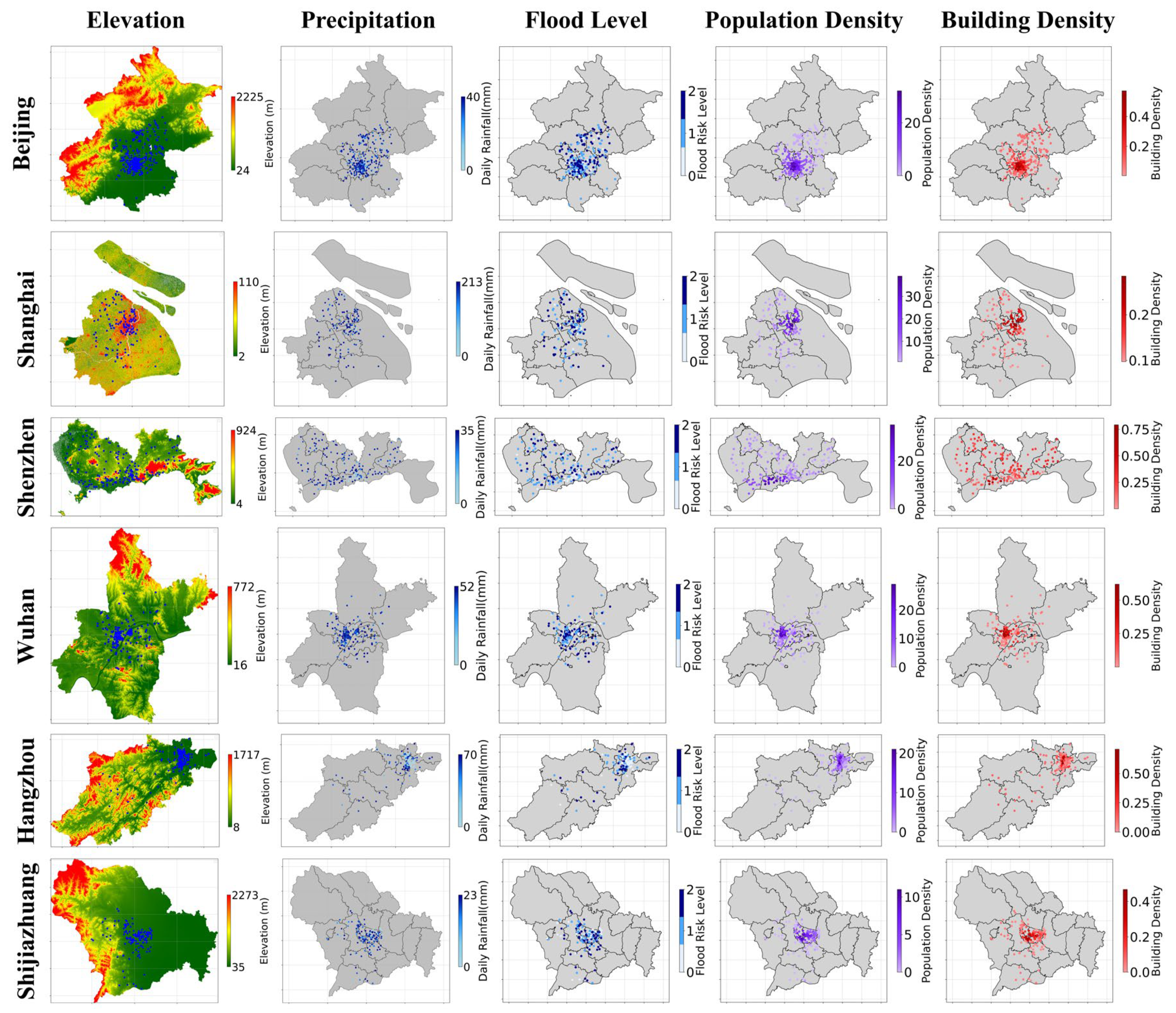
Following these steps, our mixed-city flood risk dataset is successfully created (Figure 5), comprising 1195 records from six cities within the study area (these records are displayed as small dots on the map in Figure 5 to show their specific locations). The data is categorized into three risk levels: 239 low-risk, 503 medium-risk, and 451 high-risk points. Among them, Beijing has 335 points, Shanghai 233, Shenzhen 172, Wuhan 146, Hangzhou 183, and Shijiazhuang 126. This dataset includes both static spatial features and dynamic time-series data. The static spatial features consist of geographic coordinates, elevation derived from a 30 m resolution DEM, population density, and building density, all mapped to a 30 m × 30 m grid to ensure uniformity. The dynamic time-series data includes rainfall sequences, with 48 values per record. This comprehensive dataset forms a robust basis for urban flood risk analysis and deep learning model training. Moreover, the methodology employed in this study is highly adaptable and can be extended to other social media platforms with similar characteristics, such as Twitter or Facebook, by processing and integrating the data in a comparable manner.

3. Methodology

In this study, a novel universal urban flood risk model was developed. This model integrates GCN, SNN, and PSO. As Figure 6 shows, the model’s architecture was designed to capture the complex spatiotemporal relationships in urban flooding. The GCN extracted spatial dependencies among urban nodes, while the SNN processed temporal data. PSO was utilized to optimize the model’s structure, node configuration, and hyperparameters, ensuring high efficiency and accuracy.
The model operated by first combining dynamic rainfall sequences with static features, which were then fed into a recurrent GCN to extract spatial dependencies at each time step. This generated a spatiotemporal feature sequence aligned with the rainfall input. The sequence was subsequently analyzed by the SNN for flood risk assessment. Finally, PSO was applied for global optimization of the model, enhancing its performance. The following sections will detail the design and implementation of the GCN, SNN, and PSO modules, highlighting their roles in the model.

3.1. Graph Convolutional Network

A graph convolutional network is a class of graph neural networks [33], designed to handle graph-structured data [37]. Unlike traditional convolutional neural networks, which operate on grid-like data, GCN can process non-Euclidean structures. GCNs use graph-based convolution operations to capture local dependencies between nodes. In this framework, the features of each node are influenced not only by its own attributes but also by those of its neighboring nodes. Through multiple layers of convolution, GCN iteratively aggregates information from neighboring nodes, enabling the extraction of global graph-level features.
In this study, the urban area is represented as a fully connected graph, where each node corresponds to a 30 m × 30 m city grid. For GCN input, nodes represent the grids, with their total number optimized via PSO. Each batch is created by randomly sampling nodes from the dataset, which includes data from six cities in a shuffled order, so nodes within a batch may come from different cities. This ensures that relationships between every pair of nodes are fully considered, effectively capturing spatial dependencies across urban nodes. Each node contains two types of features: static and dynamic. Static features, such as average elevation, building density, and population density, remain constant over time. Dynamic features include rainfall sequences. The edge weights between nodes are determined by geographic distance, elevation difference, and administrative boundaries:
w i j = p d d i j + p h Δ h i j + p c i t y τ i j
τ i j = { 1 , i f   i ,   j   f o r m   t h e   s a m e   c i t y   a n d   i     j 0 , o t h e r w i s e
where d i j represents the geographic distance between nodes i and j , while Δ h i j denotes the elevation difference between them. The term τ i j indicates whether nodes i and j belong to the same city, with a value of 1 if they do and 0 otherwise. The coefficients p d , p h , and p c i t y are weight parameters optimized by PSO. This graph construction approach effectively captures spatial relationships between urban grids, laying a solid foundation for subsequent graph convolution operations.
During the operation of the GCN, data is fed into the model as a time series. At each time step t , rainfall data is combined with static node features to form the input features for the GCN. Urban flood risk depends not only on the current rainfall but also on historical rainfall patterns and spatial distribution. Therefore, the model must process time-series data while capturing spatial dependencies. To achieve this, the GCN employs a recurrent graph convolution approach, performing graph convolution operations step by step over time. Specifically, at each time step t , the GCN integrates the current rainfall data with static features and updates node features through multiple convolutional layers. Each layer’s convolution operation is computed as follows:
L j + 1 = ρ A ~ L j W j
where A ~ is the normalized adjacency matrix, representing the connections between nodes. L j is the node feature matrix at the j -th layer, containing the feature representations of each node at that layer. These features incorporate both the current rainfall data and static node attributes (e.g., building density, population density), providing rich spatial information. W j is the weight matrix at the j -th layer, used to learn complex relationships between node features. In this study, the weights are determined by Equation (1). Through multiple convolutional layers, the model gradually extracts global graph features. ρ is the activation function [52], and in this study, the rectified linear unit (ReLU) is adopted for this role to introduce nonlinearity into the model and thereby enhance its expressive power.
The output of the GCN is a sequence with the same length as the input rainfall series, but each time step’s features now include extracted spatial relationships. This output sequence reflects not only the rainfall impact at each time step but also the spatial dependencies between urban blocks. Ultimately, the GCN’s output serves as the input to the SNN for further temporal feature extraction and flood risk prediction. By employing this recurrent graph convolution approach, the model effectively processes both time-series data and spatial dependencies, providing rich feature information for subsequent flood risk assessment.

3.2. Spiking Neural Network

Spiking neural networks represent the third generation of neural network models [53], emulating the natural neural network’s way of processing information through discrete spikes. Unlike traditional neural networks, SNNs process information using discrete spike signals, offering low energy consumption and excelling in handling time-series data [54]. In this study, the integration of SNN with GCN is a key innovation. Specifically, SNN processes the output of GCN, rainfall sequences enriched with spatial features, to capture temporal patterns in the data. By combining these temporal patterns with the spatial features extracted by GCN, the model generates comprehensive flood risk assessments. This integration enables the model to address the spatiotemporal complexity of urban flood risks, delivering more accurate and holistic results. Additionally, the low energy consumption of SNN, combined with the efficient spatial feature extraction of GCN, achieves a balance between computational efficiency and predictive accuracy.
Since SNNs rely on discrete spike signals and GCN outputs are continuous time-series data, a conversion from continuous data to spike signals is necessary. This transformation not only adapts the data to the SNN’s processing mechanism but also reduces computational energy consumption while preserving critical temporal information. To achieve this, Gaussian encoding [55] is employed. This probabilistic method maps feature values at each time step to binary spike sequences, where each value is represented by a series of zeros and ones. The advantage of this encoding lies in its ability to generate smooth spike signals based on the feature value distribution, effectively capturing key temporal points in the rainfall sequence. The encoding formula is as follows:
S i t = exp t μ i 2 2 σ i 2
where S i t represents the spike sequence for the i -th feature at time step t in the GCN output. μ i denotes the mean of the feature value on the time axis, determining the center of the spike signal and reflecting the distribution of key temporal points in the rainfall sequence. σ i is the standard deviation, controlling the spread of the spike signal and adjusting its intensity to adapt to feature fluctuations across time steps. This encoding method transforms continuous time-series data into discrete spike signals, providing the foundation for subsequent SNN processing.
One of the core SNNs is the Tempotron model [56], which mimics the spike generation mechanism of biological neurons. The Tempotron is chosen for its efficiency in processing time-series data and its low energy consumption, making it particularly suitable for complex spatiotemporal data. Compared to traditional neuron models, the Tempotron uses a simple threshold mechanism to generate spikes, avoiding complex computations and significantly reducing energy consumption. Moreover, its spike generation mechanism closely resembles biological neuron behavior, enabling better capture of key temporal points in the data. The spike generation condition for the Tempotron is defined as follows:
V t = i f K t t i f > θ
where V t represents the membrane potential of the neuron at time t , reflecting its current state. t i f denotes the firing time of the i -th input spike, corresponding to key temporal points in the rainfall sequence. K t t i f is the spike response function, a standard exponential decay function (as defined in [56]), describing the impact of input spikes on the membrane potential and their temporal decay. θ is the firing threshold, set to 0.5 in this study through empirical tuning on the validation dataset, which determines whether the neuron generates a spike. In this study, the input spike sequences are generated from the spatially enriched rainfall sequences output by the GCN, with t i f and K t t i f directly linked to key temporal points and their spatial dependencies. These key temporal points are autonomously extracted as data-driven features by the SNN during training and are not explicitly observable externally due to the model’s inherent “black-box” characteristics of deep learning.
After processing by the tempotron model, the SNN outputs flood risk levels (low, medium, high) for each node. Specifically, the SNN extracts temporal patterns from the spike sequences layer by layer, combining them with the spatial dependencies provided by the GCN to produce comprehensive flood risk assessments. This process not only preserves key temporal points in the rainfall sequence but also integrates spatial dependencies between urban blocks, resulting in accurate and holistic flood risk evaluations.

3.3. Particle Swarm Optimization

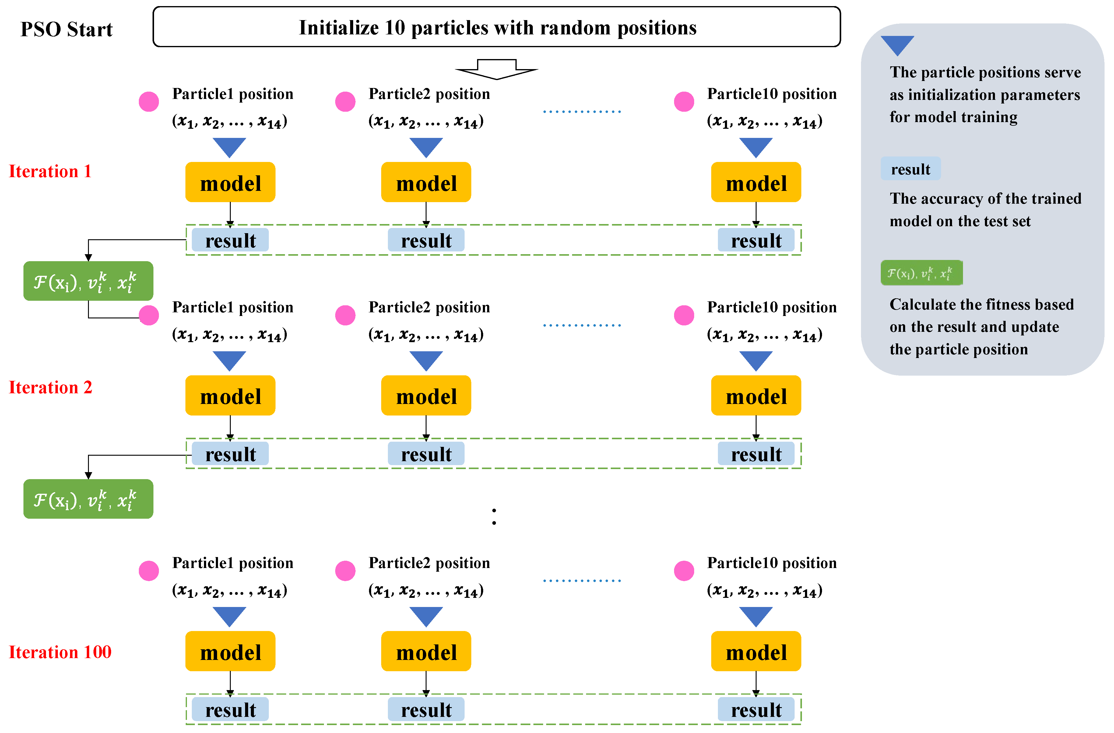
PSO is an algorithm initially inspired by the study of bird migration and foraging behavior [36]. It operates through three key components: particles (candidate solutions), a swarm (a collection of particles), and an iterative update mechanism [57]. In optimization problems, each particle explores the search space by adjusting its position based on its own experience and that of the swarm. In this study, PSO is used to optimize the parameters of the SGCN model. Each particle represents a complete model training instance, with its positional coordinates directly used as initialization parameters for model training, as illustrated in Figure 7. Once these parameters are determined through PSO, they remain fixed throughout the training process. The optimization process runs for 100 iterations, where the swarm generates 10 parallel training configurations per iteration, each undergoing a full training–validation cycle. Fitness values are computed based on the test accuracy of the trained models and used to update particle positions, refining optimization parameters for the next training cycle.
The first step in PSO implementation is defining the search space, which determines the range of possible solutions. Based on the operational principles of the SGCN model, we establish a 14-parameter optimization space (Table 3). These parameters collectively determine the model’s performance. The graph structure parameters ( p g r a p h n , p d , p h , p c i t y ) define the granularity of spatial topology capture by adjusting the input graph’s node size and edge weight coefficients. The GCN parameters ( p g c n n , p g c n h i d ) control the depth and feature representation capacity of the GCN. The SNN parameters ( p s n n n , p m , p T , p τ , p τ s ) shape the structure and temporal dynamics of the SNN. The training hyperparameters ( p e p o c h , p b a t c h , p l r ) regulate training efficiency and convergence.
In PSO, the fitness function quantifies the quality of each particle’s solution, guiding the optimization process by influencing particle updates. It serves as a performance metric to assess candidate parameters. In this study, the fitness function is derived from the test accuracy of trained models, as follows:
F x i = 1 A c c u r a c y t e s t
where A c c u r a c y t e s t is the model’s accuracy on the test set for the given parameter configuration, calculated as the number of correctly classified flood levels divided by the total size of the test set. By minimizing F x i , PSO effectively maximizes model accuracy. Each particle position x i R 14 represents a complete SGCN parameter set, aligning with the 14-dimensional search space in Table 3. The particle update equations are defined as follows:
v i k = w v i k 1 + c 1 r 1 p b e s t i k x i k + c 2 r 2 g b e s t k x i k
x i k = x i k 1 + v i k
where k is the iteration step. The inertia weight ω 0.4,0.9 controls velocity retention. The cognitive and social factors c 1 , c 2 balance individual learning and swarm intelligence. Random terms r 1 , r 2 U 0,1 ensure population diversity. The best individual position p b e s t i k and the global best position g b e s t k , both evaluated via F x i , drive the swarm towards high-performance regions.

3.4. Experimental Setup

In the experiments, aLenovo high-performance server equipped with Ubuntu 22.04.3 Long-Term Support, two Intel(R) Xeon(R) Gold 6271C central processing units (CPU), 256 GB of random access memory (RAM), and eight NVIDIA Ray Tracing Texel Xtreme 3090 graphics processing units (GPUs) was employed. The software environment comprised the PyTorch 2.4.1 [58] and SpikingJelly 0.0.0.0.14 [59] deep learning frameworks. Initially, the mixed-city flood risk dataset was randomized using a consistent random seed to ensure integrity and mitigate bias, dividing it into 80% for training and 20% for testing. This process, facilitated by a fixed random seed set to zero, allowed for reproducible dataset splits across various experimental runs.
The PSO algorithm utilizes default parameters ( c 1 = c 2 = 1.5, w = 0.9) following standard practice. This study conducted 100 iterations with a 10-particle swarm and performed 10 randomized trials, resulting in 10,000 model evaluations (10 trials × 10 particles × 100 iterations) to systematically explore the parameter space. Multithreaded parallel computation is implemented to execute concurrent training instances, accelerating the optimization process for the SGCN model. After applying PSO, an optimal architecture for the SGCN model is established, consisting of four GCN layers and three SNN layers. To ensure a fair comparison of computational complexity, baseline models are designed with seven-layer architectures: the GCN baseline stacks seven GCN layers (256 hidden units, batch normalization, and residual connections) followed by global pooling, while the LSTM baseline employs a seven-layer bidirectional structure (256 hidden units per layer, dropout rate = 0.2) enhanced with temporal attention mechanisms. Both baselines were tuned via grid search (adjusting hidden unit counts, dropout rates, and learning rates) through dozens of training runs to select validation-set optimal configurations. All models are trained under identical conditions, including input features, dataset partitioning, and hardware configurations. Their performance is evaluated on the same test set using precision, recall, f1 score, accuracy, precision–recall area under the curve (PR-AUC), receiver operating characteristic area under the curve (ROC-AUC), and energy efficiency metrics:
Precision = T P T P + F P
Recall = T P T P + F N
F 1 S core = 2 × Precision × Recall Precision + Recall
Accuracy = T P + T N T P + F P + F N + T N
PR AUC = m = 1 n 1 Recall m + 1 Recall m Precision m + Precision m + 1 2
R O C A U C = 1 N + N [ i = 1 N + j = 1 N I ( score i > score j ) + 1 2 i = 1 N + j = 1 N I ( score i = score j ) ]
where TP is true positives (correctly predicted urban flood levels), FP is false positives (incorrectly predicted urban flood levels), TN is true negatives (correctly predicted absence of specific urban flood levels), and FN is false negatives (missed predictions of actual urban flood levels). In Equation (13), n = number of sampling points on the precision–recall curve; Recall m , Recall m + 1 = recall values at the m-th and (m + 1)-th points; and Precision m , Precision m + 1 = precision values at the m-th and (m + 1)-th points. In Equation (14), N + = number of positive samples; N = number of negative samples; score i , score j = model confidence scores for the i-th positive and j-th negative samples; and I = indicator function (1 if true, 0 otherwise). All are count values representing the number of samples in each classification category for the three urban flood levels.
Sensitivity analysis is crucial to understanding how input features influence model predictions, especially when evaluating complex models for urban flood risk. This study applies feature perturbation [60,61] to quantify the sensitivity of three models, P-SGCN, GCN, and LSTM, to variations in time series, static spatial, and spatial topology features. Time series features (rainfall data) are perturbed by adding Gaussian noise with a standard deviation of 10% of the original value. Static spatial features (population and building density) are disturbed by random variations within ±5%, and spatial topology features (elevation and proximity relationships) are adjusted by altering elevation values within ±5% and randomly removing 10% of adjacency edges. The sensitivity of each model is measured by calculating the mean absolute level difference (MAE) between the original and perturbed outputs, which is calculated according to the following equation:
S e n s i t i v i t y   S c o r e = 1 N i = 1 N Level original i Level perturbed i
where Level original   i and Level perturbed   i are the outputs of the i -th data point before and after perturbation, respectively, and N is the total number of data points.
An additional experiment was conducted to validate the models’ performance on real-world data. The study used flood risk data from Dongguan city on 21 August 2024, which consists of 65 monitoring stations with actual hourly water depth measurements. The data processing followed the same methodology as the self-constructed dataset in this research, with the only difference being that the flood risk classification was based on the maximum water depth recorded on that day. This setup was used to test the models’ ability to predict flood risk under real urban flooding conditions, offering an external validation of their effectiveness.
As the demand for sustainable computational models continues to escalate, energy efficiency has become a crucial metric for determining a model’s suitability for large-scale applications. In the experimental section, this study also compares the energy consumption and the number of parameters of the GCN, LSTM, and P-SGCN models. To further explore the generalization capability of the improved P-SGCN model, transfer learning is applied. The pre-trained P-SGCN model is tested on single-city data while maintaining the original dataset structure, with inputs corresponding to the specific city. During transfer learning, only the final layer of the SNN component is unfrozen, while all initial parameters remain unchanged, ensuring consistency with the original model configuration.

4. Results and Discussion

4.1. Parameter Optimization with P-SGCN Model Performance

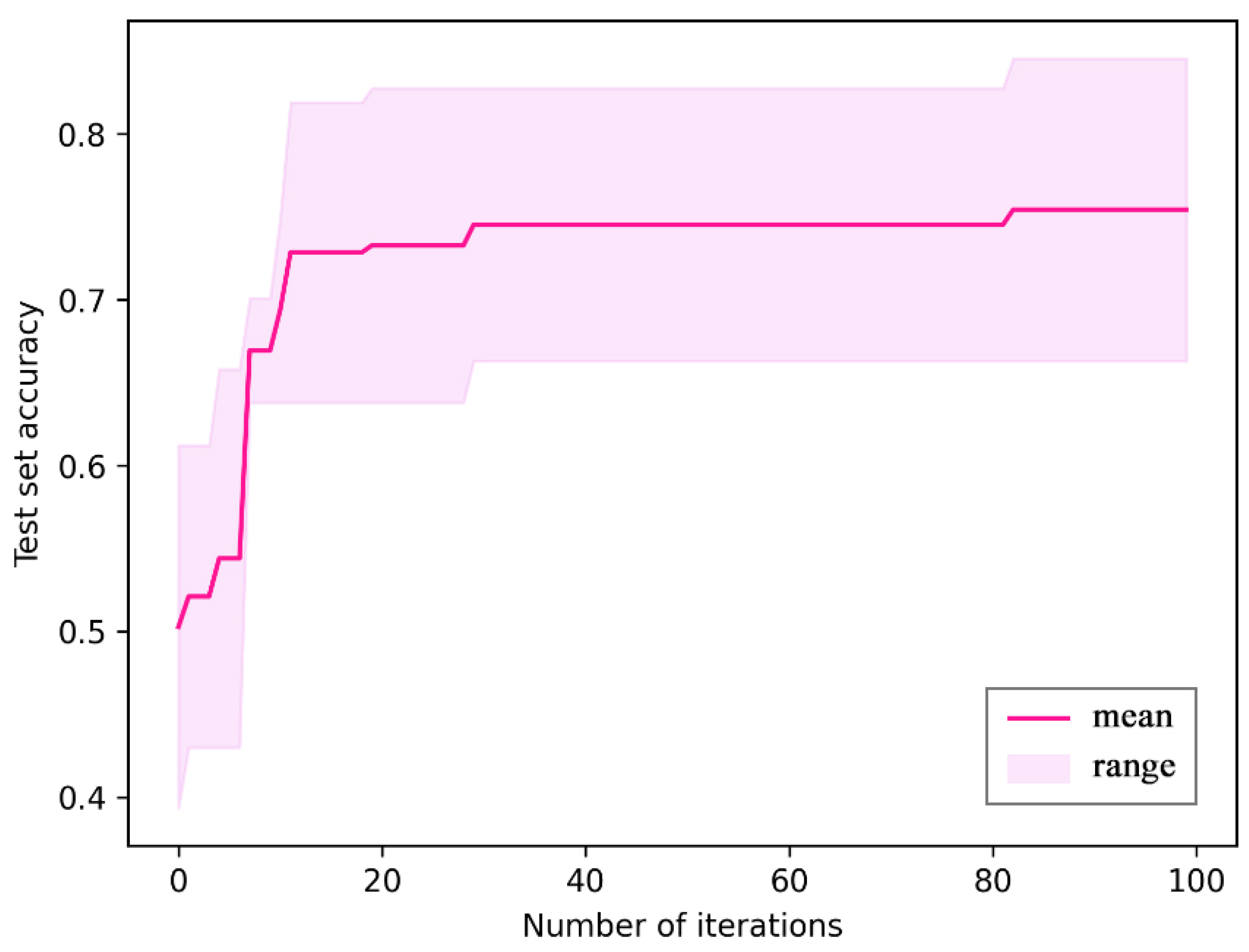
PSO demonstrated effective convergence during parameter tuning. The convergence curve (Figure 8) shows that across 10 randomized trials, the highest accuracy reached 84.56%, while the lowest accuracy was 68.2%. The middle trajectory indicates a consistent upward trend in average performance as iterations increased. All runs converged after approximately 80 iterations, where particles stabilized at a common optimal position, confirming convergence stability. Table 4 lists the optimized hyperparameters generated by PSO, showing precise tuning across both structural and training parameters of the SGCN. The optimized values differ significantly from the initial configuration, especially in floating-point parameters, which were fine-adjusted to the third decimal place. This indicates that PSO achieved refined parameter calibration. With PSO applied, the model parameters were adjusted to better fit complex urban flood datasets.

4.2. Performance Results of Different Models

Figure 9 compares the performance of GCN, LSTM, and P-SGCN on urban flood test sets from six cities. Across all datasets, P-SGCN achieved the highest accuracy, while LSTM exhibited the lowest. The confusion matrices in Figure 10 show that P-SGCN achieved classification accuracies of 0.836, 0.855, and 0.841 for low-, medium-, and high-risk classes.
Table 5 further summarizes the quantitative evaluation metrics, where P-SGCN ranked highest in precision, recall, f1 score, PR-AUC, and ROC-AUC. In comparison, LSTM showed the weakest performance across all metrics, while GCN performed notably better than LSTM on each indicator but still fell short of the proposed P-SGCN.
Table 6 presents the feature sensitivity scores for each model. GCN showed higher sensitivity to elevation and proximity, while LSTM responded most strongly to precipitation. In contrast, P-SGCN demonstrated balanced sensitivity across both spatial and temporal inputs—not in terms of numerical range but in maintaining comparable responsiveness to both feature types, reflecting its ability to integrate spatiotemporal information more effectively.
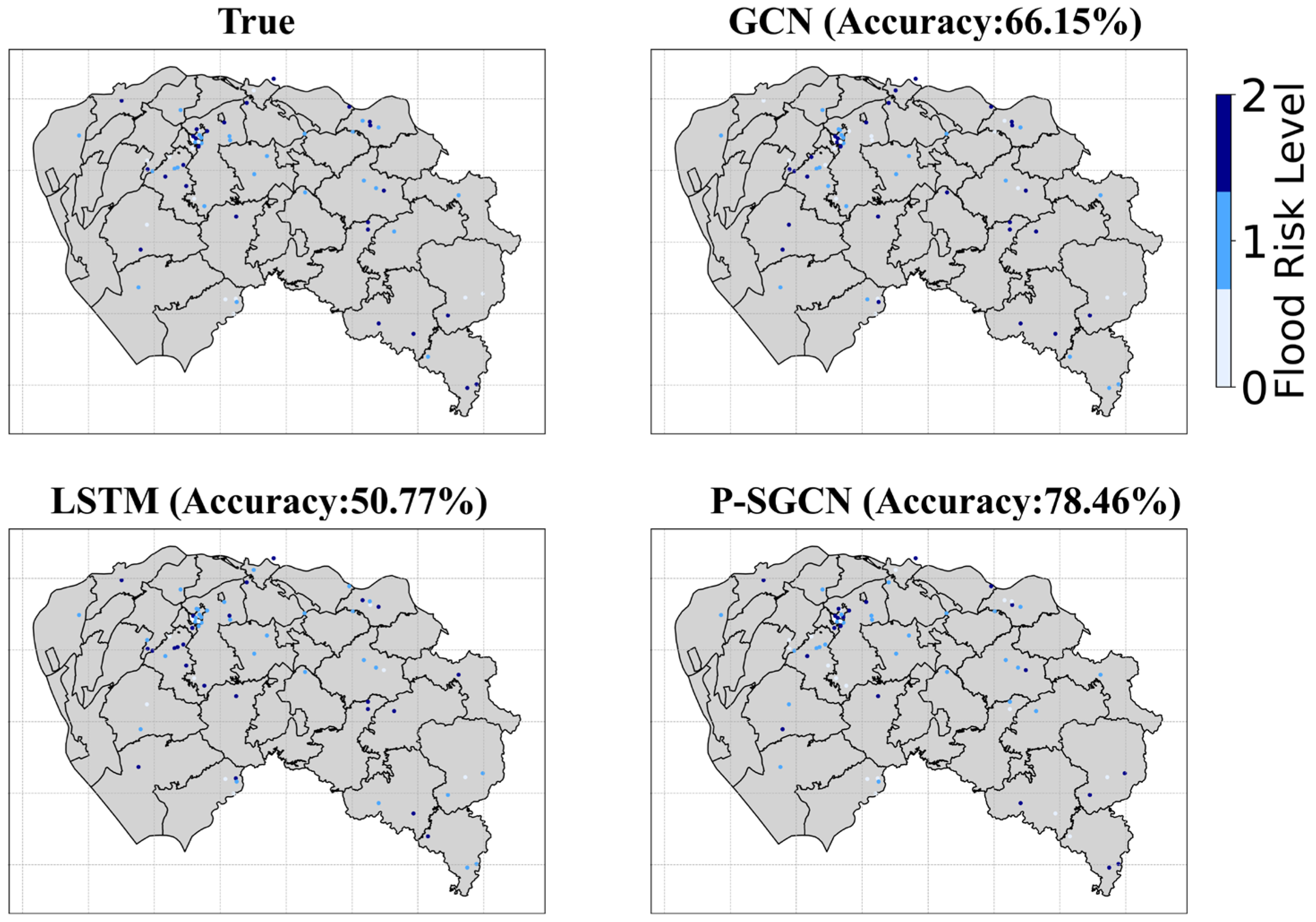
Figure 11 shows the application of the three models on Dongguan flood data, with their predicted flood risk overlaid on actual flood maps. P-SGCN achieves the highest accuracy (78.46%), followed by GCN (66.15%) and LSTM (50.77%).

4.3. Energy Consumption and Parameters of Different Models

Table 7 reports the energy consumption and parameter count of the three models. P-SGCN consumed a total of 11.9 J, which was lower than both GCN (53.5 J) and LSTM (20.4 J). In addition, P-SGCN contained only 1.31 million parameters compared to 2.06 million for GCN and 2.37 million for LSTM. The memory and computation usage recorded for RAM, CPU, and GPU show that P-SGCN required less computational overhead for inference compared with the other models.

4.4. P-SGCN Model Adaptation via Transfer Learning

Table 8 presents the transfer learning results. Transfer learning refers to the process of adapting a pre-trained model from one domain (source city) to another related domain (target city) to improve performance with limited local data. The results were evaluated using accuracy, defined as the proportion of correctly classified urban flood risk samples in each city. The universal model achieved accuracy values ranging from 0.809 to 0.869 across different cities. After transfer learning adjustment, accuracy increased for all cities, with improvements observed for Beijing (0.865→0.904), Shanghai (0.853→0.892), and Wuhan (0.817→0.878). Shenzhen and Shijiazhuang showed marginal changes after transfer, indicating that the universal model already aligned well with their data patterns.

5. Discussion

5.1. Impact of PSO on Model Stability and Optimization Efficiency

The optimization results indicate that PSO significantly enhances the stability and convergence efficiency of the SGCN model, consistent with findings from recent research on metaheuristic optimization in deep learning [62,63,64]. The rapid convergence observed around the 80th iteration suggests that the algorithm can consistently locate a global optimum with minimal fluctuations, even under randomized initialization. Unlike conventional grid or random search methods, PSO dynamically balances exploration and exploitation, which explains its superior convergence behavior in high-dimensional spatiotemporal parameter spaces. This stable convergence pattern reduces reliance on manual hyperparameter tuning, making the training process more reproducible and scalable across different datasets and deployment environments. This finding extends previous studies, which primarily verified PSO’s efficiency in image or signal domains, by demonstrating its capability to stabilize learning in graph-based spiking architectures—a setting not previously explored.
The fine-grained adjustment of continuous parameters to the third decimal place demonstrates PSO’s ability to explore the hyperparameter space efficiently, even when handling nonlinear spatiotemporal dependencies. Parameter adaptation is essential for hybrid models, especially those that combine both spatial graph convolutions and temporally sensitive mechanisms [63]. Our results further reveal that PSO’s global search property reduces the risk of overfitting in spatiotemporal tasks by maintaining smoother parameter landscapes during optimization. For spatiotemporal flood risk modeling, where rainfall intensity, runoff accumulation, and urban drainage response interact in complex ways, this precise optimization capability enables the model to better align with real-world data dynamics. This complements and refines previous optimization-focused studies that did not consider the chaotic and non-stationary nature of hydrological data, showing that PSO can serve as a general mechanism to enhance model interpretability and stability under environmental uncertainty.

5.2. Interpretation of Cross-Model Performance Differences

The superior performance of P-SGCN compared with GCN and LSTM validates the benefit of combining spatial topology learning with spiking-based temporal feature extraction. Unlike prior approaches that treated spatial and temporal dependencies as independent modules, our results show that their joint representation leads to synergistic improvement rather than additive gains. P-SGCN outperforms both baselines by integrating GCN’s spatial representational power with the spike-based temporal encoding of SNN. This hybrid mechanism allows the model to simultaneously track spatial clustering of flood signals and spike-driven temporal surges in rainfall-induced runoff. Our results demonstrate, for the first time, that event-based spike encoding can capture temporal accumulation effects in environmental processes without relying on dense recurrent structures, offering a more biologically inspired and energy-efficient alternative.
Such coupled learning reflects the physical process of urban flooding, where localized topographic depressions, road networks, and stormwater drainage interact with the temporal evolution of precipitation. This integrated spatiotemporal learning not only aligns model behavior with hydrological theory but also addresses the interpretability gap observed in purely data-driven models. In alignment with the sustainable development goal “Sustainable Cities and Communities,” this approach promotes adaptive resilience by enabling decentralized flood warning strategies that respond dynamically to evolving urban conditions. Overall, the P-SGCN architecture contributes a novel theoretical link between spiking dynamics and urban hydrology, providing a foundation for interpretable, cross-domain environmental AI systems.

5.3. Energy Efficiency and Lightweight Architecture Advantages

Energy efficiency and architectural compactness are increasingly important in the deployment of deep-learning-based early warning systems. A core finding of this study is that event-driven spiking computation can substantially reduce inference energy without sacrificing predictive accuracy. Compared with conventional GCN and LSTM baselines, P-SGCN attains a markedly lower energy profile through sparse, spike-triggered activations rather than dense matrix operations. This demonstrates that energy-efficient architectures are not only feasible for spatiotemporal flood modeling but can also maintain or improve performance—contradicting a common implicit assumption in prior work that efficiency necessarily trades off with accuracy.
This energy–accuracy coupling has practical implications and refines existing knowledge: lightweight, low-energy models like P-SGCN are better suited for edge and municipal deployments where power and compute are constrained, enabling continuous, real-time flood monitoring that was previously impractical with heavy models.

5.4. Transfer Learning and Model Adaptability Across Cities

The transfer learning results demonstrate that while the universal P-SGCN model achieves strong performance across diverse urban settings, localized fine-tuning significantly enhances prediction accuracy in cities with complex hydrological dynamics or sparse crowdsourced flood data. This finding reveals that universal flood models, though robust, must still adapt to micro-level hydrological differences to reach operational precision. By confirming these domain-specific adjustments, our results correct a common misconception in previous cross-city flood research—that universal models alone can fully generalize without adaptation.
In contrast, cities like Shenzhen, with more uniform urban layouts and consistent rainfall-drainage behavior, benefit less from transfer learning. This indicates that model adaptability should follow a selective adaptation strategy, where transfer learning resources are prioritized for morphologically complex or data-scarce regions. Our findings refine the current understanding of model transferability, suggesting that the effectiveness of transfer learning is governed not only by data volume but by the hydrological diversity of the target city. Although this study’s experiments were conducted in China, the P-SGCN architecture demonstrates clear global applicability. With modular data ingestion, social sensing inputs can be replaced with other region-specific information sources such as Twitter feeds, Facebook crisis alerts, or sensor-based flood reports. This adaptability distinguishes P-SGCN from earlier localized models, positioning it as a scalable foundation for multi-region flood intelligence systems.

5.5. Practical Implications, Data Reliability, and Future Research Directions

The results confirm that P-SGCN holds strong potential for integration into operational urban flood warning systems. Its capability to deliver high accuracy with a low computational cost positions it as a viable core module for smart city flood intelligence platforms. Practically, this means that municipal centers could implement real-time flood prediction even under limited computational conditions, advancing the feasibility of AI-driven disaster management in developing regions. Furthermore, the model’s demonstrated transferability implies that a single globally trained model could be maintained as a centralized foundation and gradually adapted to local conditions through incremental fine-tuning. This paradigm bridges global modeling and local adaptation, offering a path toward federated, continuously learning environmental AI systems.
However, challenges remain in the reliability of crowdsourced flood indicators. User-generated data present biases in spatial reporting, timestamp accuracy, and perception of severity [65]. Despite the filtering pipeline applied in this study, unstructured social media data can be subject to overreporting in densely populated commercial zones and underreporting in marginalized or low-connectivity neighborhoods. This limitation underscores that social-sensing data should serve as a complementary, not primary, layer in multi-source flood monitoring frameworks. Future research should incorporate multimodal fusion strategies integrating remote sensing, weather radar, unmanned aerial vehicle imagery, and hydrological sensor networks. Additionally, continual learning could allow the model to adjust automatically to infrastructure changes and shifting climate baselines, ensuring long-term reliability.

6. Conclusions

This study presents P-SGCN, a universal model for urban flood risk assessment across multiple cities. By jointly modeling spatial and temporal dependencies, P-SGCN significantly outperforms baseline models, achieving an accuracy, precision, recall, and F1 score of 0.8456, 0.8474, 0.8456, and 0.8458, respectively. Its performance was validated using a self-constructed mixed-city flood risk dataset and further confirmed through real-world testing in Dongguan, demonstrating strong robustness and generalizability. The results highlight that flood risk mapping benefits from integrating spatial–temporal features, particularly proximity relationships and elevation variations, as shown by sensitivity analysis. The model also underscores the secondary but notable influence of population and building density, offering valuable insights for flood mitigation and resilience planning.
The integration of PSO effectively enhances model accuracy and computational efficiency. By systematically tuning key parameters, PSO enables P-SGCN to achieve high performance while maintaining a low computational cost. The model’s total energy consumption is only 11.9 J, considerably lower than that of conventional models, making it suitable for real-time flood prediction. Transfer learning further demonstrates the model’s adaptability, allowing efficient fine-tuning for specific cities while preserving generalization capability. These features establish P-SGCN as a scalable solution for diverse urban environments.
Despite its strengths, several limitations remain. The reliance on social-media-derived flood data may introduce biases, as data quality and availability differ by region. Moreover, while the model generalizes well across six Chinese cities, further validation is required in areas with different climatic and urban conditions. The use of local rainfall data, though suitable for pluvial flooding, may not capture fluvial dynamics influenced by upstream rainfall. Future research should refine data integration, incorporate broader environmental and hydrological variables, and extend validation to global cities. Enhancing real-time processing and optimizing large-scale deployment will further improve practical applicability in disaster management and urban planning.
By addressing key challenges in flood risk assessment with a scalable, efficient, and adaptable framework, this study contributes to improving global urban flood resilience. Beyond technical advances, P-SGCN has strong policy relevance—supporting dynamic flood zoning, informed resource allocation, and real-time decision-making for emergency response. Its low energy use and deployability on edge devices align with green AI principles, making it ideal for integration into sustainable urban infrastructure and smart city resilience systems. Ultimately, P-SGCN serves not only as a computational model but also as a strategic tool for data-driven urban governance, disaster preparedness, and long-term sustainable development, with practical applications for urban planning agencies, water authorities, emergency management, smart city centers, insurance institutions, and community response units.

Author Contributions

X.F.: Conceptualization, Methodology, Software, Formal analysis, Investigation, Resources, Writing—original draft, Visualization. J.L.: Conceptualization, Methodology, Writing—review and editing, Resources, Supervision, Project administration, Funding acquisition. M.W.: Investigation, Writing—review and editing. A.C.: Conceptualization, Writing—review and editing. S.S.: Conceptualization, Writing–review and editing, Resources, Supervision. Q.L.: Formal analysis, Visualization. All authors have read and agreed to the published version of the manuscript.

Funding

This work was supported by the National Key Research and Development Program of China (2023YFC3206700), the National Natural Science Foundation of China (No. 52109079), the Guangdong Provincial Key Laboratory of Intelligent Disaster Prevention and Emergency Technologies for Urban Lifeline Engineering (2022B1212010016). The authors would also like to express their sincere gratitude to the Dongguan Meteorological Bureau for providing the measured urban flooding data in Dongguan.

Institutional Review Board Statement

Not applicable.

Informed Consent Statement

Not applicable.

Data Availability Statement

Data will be made available on request.

Conflicts of Interest

The authors declare that they have no known competing financial interests or personal relationships that could have appeared to influence the work reported in this paper.

References

  1. Jongman, B.; Hochrainer-Stigler, S.; Feyen, L.; Aerts, J.C.; Mechler, R.; Botzen, W.W.; Bouwer, L.M.; Pflug, G.; Rojas, R.; Ward, P.J. Increasing Stress on Disaster-Risk Finance Due to Large Floods. Nat. Clim. Change 2014, 4, 264–268. [Google Scholar] [CrossRef]
  2. Pourghasemi, H.R.; Gayen, A.; Panahi, M.; Rezaie, F.; Blaschke, T. Multi-Hazard Probability Assessment and Mapping in Iran. Sci. Total Environ. 2019, 692, 556–571. [Google Scholar] [CrossRef]
  3. Rahmati, O.; Darabi, H.; Panahi, M.; Kalantari, Z.; Naghibi, S.A.; Ferreira, C.S.S.; Kornejady, A.; Karimidastenaei, Z.; Mohammadi, F.; Stefanidis, S. Development of Novel Hybridized Models for Urban Flood Susceptibility Mapping. Sci. Rep. 2020, 10, 12937. [Google Scholar] [CrossRef]
  4. Rusk, J.; Maharjan, A.; Tiwari, P.; Chen, T.-H.K.; Shneiderman, S.; Turin, M.; Seto, K.C. Multi-Hazard Susceptibility and Exposure Assessment of the Hindu Kush Himalaya. Sci. Total Environ. 2022, 804, 150039. [Google Scholar] [CrossRef]
  5. Yousefi, S.; Pourghasemi, H.R.; Rahmati, O.; Keesstra, S.; Emami, S.N.; Hooke, J. Geomorphological Change Detection of an Urban Meander Loop Caused by an Extreme Flood Using Remote Sensing and Bathymetry Measurements (a Case Study of Karoon River, Iran). J. Hydrol. 2021, 597, 125712. [Google Scholar] [CrossRef]
  6. Wang, Y.; Xie, X.; Liang, S.; Zhu, B.; Yao, Y.; Meng, S.; Lu, C. Quantifying the Response of Potential Flooding Risk to Urban Growth in Beijing. Sci. Total Environ. 2020, 705, 135868. [Google Scholar] [CrossRef]
  7. Wang, H.; Hu, Y.; Guo, Y.; Wu, Z.; Yan, D. Urban Flood Forecasting Based on the Coupling of Numerical Weather Model and Stormwater Model: A Case Study of Zhengzhou City. J. Hydrol. Reg. Stud. 2022, 39, 100985. [Google Scholar] [CrossRef]
  8. Ziegler, A.D.; She, L.H.; Tantasarin, C.; Jachowski, N.R.; Wasson, R. Floods, False Hope, and the Future. Hydrol. Process. 2012, 26, 1748–1750. [Google Scholar] [CrossRef]
  9. Wang, M.; Fu, X.; Zhang, D.; Chen, F.; Liu, M.; Zhou, S.; Su, J.; Tan, S.K. Assessing Urban Flooding Risk in Response to Climate Change and Urbanization Based on Shared Socio-Economic Pathways. Sci. Total Environ. 2023, 880, 163470. [Google Scholar] [CrossRef]
  10. Chen, Z.; Fang, X.; Li, J.; Wang, M.; Chen, A.; Yin, L. An Overview of Application of Machine Learning Models in Urban Flood Simulation and Forecasting. Pearl River 2025, 46, 9–22. [Google Scholar] [CrossRef]
  11. Liao, Y.; Wang, Z.; Chen, X.; Lai, C. Fast Simulation and Prediction of Urban Pluvial Floods Using a Deep Convolutional Neural Network Model. J. Hydrol. 2023, 624, 129945. [Google Scholar] [CrossRef]
  12. Mignot, E.; Dewals, B. Hydraulic Modelling of Inland Urban Flooding: Recent Advances. J. Hydrol. 2022, 609, 127763. [Google Scholar] [CrossRef]
  13. Wang, Y.; Zhang, Q.; Lin, K.; Liu, Z.; Liang, Y.; Liu, Y.; Li, C. A Novel Framework for Urban Flood Risk Assessment: Multiple Perspectives and Causal Analysis. Water Res. 2024, 256, 121591. [Google Scholar] [CrossRef]
  14. Mukerji, A.; Chatterjee, C.; Raghuwanshi, N.S. Flood Forecasting Using ANN, Neuro-Fuzzy, and Neuro-GA Models. J. Hydrol. Eng. 2009, 14, 647–652. [Google Scholar] [CrossRef]
  15. Mudashiru, R.B.; Sabtu, N.; Abustan, I.; Balogun, W. Flood Hazard Mapping Methods: A Review. J. Hydrol. 2021, 603, 126846. [Google Scholar] [CrossRef]
  16. Wang, Y.; Zhang, Q.; Zhang, J.; Lin, K. Impact of 2D and 3D Factors on Urban Flooding: Spatial Characteristics and Interpretable Analysis of Drivers. Water Res. 2025, 280, 123537. [Google Scholar] [CrossRef]
  17. Jodar-Abellan, A.; Valdes-Abellan, J.; Pla, C.; Gomariz-Castillo, F. Impact of Land Use Changes on Flash Flood Prediction Using a Sub-Daily SWAT Model in Five Mediterranean Ungauged Watersheds (SE Spain). Sci. Total Environ. 2019, 657, 1578–1591. [Google Scholar] [CrossRef]
  18. Devia, G.K.; Ganasri, B.P.; Dwarakish, G.S. A Review on Hydrological Models. Aquat. Procedia 2015, 4, 1001–1007. [Google Scholar] [CrossRef]
  19. Gironás, J.; Roesner, L.A.; Rossman, L.A.; Davis, J. A New Applications Manual for the Storm Water Management Model (SWMM). Environ. Model. Softw. 2010, 25, 813–814. [Google Scholar] [CrossRef]
  20. Xia, X.; Liang, Q.; Ming, X. A Full-Scale Fluvial Flood Modelling Framework Based on a High-Performance Integrated Hydrodynamic Modelling System (HiPIMS). Adv. Water Resour. 2019, 132, 103392. [Google Scholar] [CrossRef]
  21. Mesa-Mingorance, J.L.; Ariza-López, F.J. Accuracy Assessment of Digital Elevation Models (DEMs): A Critical Review of Practices of the Past Three Decades. Remote Sens. 2020, 12, 2630. [Google Scholar] [CrossRef]
  22. Teng, J.; Jakeman, A.J.; Vaze, J.; Croke, B.F.; Dutta, D.; Kim, S. Flood Inundation Modelling: A Review of Methods, Recent Advances and Uncertainty Analysis. Environ. Model. Softw. 2017, 90, 201–216. [Google Scholar] [CrossRef]
  23. Yatsalo, B.; Radaev, A.; Martínez, L. From MCDA to Fuzzy MCDA: Presumption of Model Adequacy or Is Every Fuzzification of an mCDA Method Justified? Inf. Sci. 2022, 587, 371–392. [Google Scholar] [CrossRef]
  24. Bączkiewicz, A.; Wątróbski, J.; Kizielewicz, B.; Sałabun, W. Towards Objectification of Multi-Criteria Assessments: A Comparative Study on MCDA Methods. In Proceedings of the 2021 16th Conference on Computer Science and Intelligence Systems (FedCSIS), Sofia, Bulgaria, 2–5 September 2021; pp. 417–425. [Google Scholar]
  25. Lin, L.; Tang, C.; Liang, Q.; Wu, Z.; Wang, X.; Zhao, S. Rapid Urban Flood Risk Mapping for Data-Scarce Environments Using Social Sensing and Region-Stable Deep Neural Network. J. Hydrol. 2023, 617, 128758. [Google Scholar] [CrossRef]
  26. Fu, G.; Jin, Y.; Sun, S.; Yuan, Z.; Butler, D. The Role of Deep Learning in Urban Water Management: A Critical Review. Water Res. 2022, 223, 118973. [Google Scholar] [CrossRef]
  27. Li, C.; Sun, N.; Lu, Y.; Guo, B.; Wang, Y.; Sun, X.; Yao, Y. Review on Urban Flood Risk Assessment. Sustainability 2022, 15, 765. [Google Scholar] [CrossRef]
  28. Farahmand, H.; Xu, Y.; Mostafavi, A. A Spatial–Temporal Graph Deep Learning Model for Urban Flood Nowcasting Leveraging Heterogeneous Community Features. Sci. Rep. 2023, 13, 6768. [Google Scholar] [CrossRef]
  29. Guo, K.; Guan, M.; Yu, D. Urban Surface Water Flood Modelling–a Comprehensive Review of Current Models and Future Challenges. Hydrol. Earth Syst. Sci. 2021, 25, 2843–2860. [Google Scholar] [CrossRef]
  30. Karmegam, D.; Ramamoorthy, S.; Mappillairaju, B. Near Real Time Flood Inundation Mapping Using Social Media Data as an Information Source: A Case Study of 2015 Chennai Flood. Geoenviron. Disasters 2021, 8, 25. [Google Scholar] [CrossRef]
  31. Young, J.C.; Arthur, R.; Spruce, M.; Williams, H.T. Social Sensing of Flood Impacts in India: A Case Study of Kerala 2018. Int. J. Disaster Risk Reduct. 2022, 74, 102908. [Google Scholar] [CrossRef]
  32. Wang, Y. Medieval Chinese Autobiographical Writing: The Self-Written Epitaph. Mediev. Hist. J. 2015, 18, 305–345. [Google Scholar] [CrossRef]
  33. Kipf, T.N.; Welling, M. Semi-Supervised Classification with Graph Convolutional Networks. In Proceedings of the 5th International Conference on Learning Representations (ICLR 2017), Toulon, France, 24–26 April 2017. [Google Scholar]
  34. Zhang, S.; Tong, H.; Xu, J.; Maciejewski, R. Graph Convolutional Networks: A Comprehensive Review. Comput. Soc. Netw. 2019, 6, 11. [Google Scholar] [CrossRef] [PubMed]
  35. Tavanaei, A.; Ghodrati, M.; Kheradpisheh, S.R.; Masquelier, T.; Maida, A. Deep Learning in Spiking Neural Networks. Neural Netw. 2019, 111, 47–63. [Google Scholar] [CrossRef] [PubMed]
  36. Kennedy, J.; Eberhart, R. Particle Swarm Optimization. In Proceedings of the ICNN’95—International Conference on Neural Networks, Perth, WA, Australia, 27 November–1 December 1995; Volume 4, pp. 1942–1948. [Google Scholar]
  37. Khemani, B.; Patil, S.; Kotecha, K.; Tanwar, S. A Review of Graph Neural Networks: Concepts, Architectures, Techniques, Challenges, Datasets, Applications, and Future Directions. J. Big Data 2024, 11, 18. [Google Scholar] [CrossRef]
  38. Taherkhani, A.; Belatreche, A.; Li, Y.; Cosma, G.; Maguire, L.P.; McGinnity, T.M. A Review of Learning in Biologically Plausible Spiking Neural Networks. Neural Netw. 2020, 122, 253–272. [Google Scholar] [CrossRef]
  39. Lorenzo, P.R.; Nalepa, J.; Kawulok, M.; Ramos, L.S.; Pastor, J.R. Particle Swarm Optimization for Hyper-Parameter Selection in Deep Neural Networks. In Proceedings of the Genetic and Evolutionary Computation Conference, Berlin, Germany, 15–19 July 2017; ACM: Berlin, Germany, 2017; pp. 481–488. [Google Scholar]
  40. Boyarskikh, K.A.; Khishchenko, K.V. Algorithm for Finding Parameters of Equations of State by Particle Swarm Optimization. Bull. Russ. Acad. Sci. Phys. 2024, 88, 1446–1451. [Google Scholar] [CrossRef]
  41. Yin, K.; Ma, J.; Mostafavi, A. Unsupervised Graph Deep Learning Reveals Emergent Flood Risk Profile of Urban Areas. arXiv 2023, arXiv:2309.14610. [Google Scholar] [CrossRef]
  42. Zhang, L.; Qin, H.; Mao, J.; Cao, X.; Fu, G. High Temporal Resolution Urban Flood Prediction Using Attention-Based LSTM Models. J. Hydrol. 2023, 620, 129499. [Google Scholar] [CrossRef]
  43. Zhao, Z.; Alzubaidi, L.; Zhang, J.; Duan, Y.; Gu, Y. A Comparison Review of Transfer Learning and Self-Supervised Learning: Definitions, Applications, Advantages and Limitations. Expert. Syst. Appl. 2023, 242, 122807. [Google Scholar] [CrossRef]
  44. Qin, D.; Tao, S.; Dong, S.; Luo, Y. Climate, Environmental, and Socioeconomic Characteristics of China. In Climate and Environmental Change in China: 1951–2012; Qin, D., Ding, Y., Mu, M., Eds.; Springer: Berlin/Heidelberg, Germany, 2016; pp. 1–27. ISBN 978-3-662-48480-7. [Google Scholar]
  45. Hou, H.; Shen, L.; Jia, J.; Xu, Z. An Integrated Framework for Flood Disaster Information Extraction and Analysis Leveraging Social Media Data: A Case Study of the Shouguang Flood in China. Sci. Total Environ. 2024, 949, 174948. [Google Scholar] [CrossRef]
  46. Zeng, Z.; Lan, J.; Hamidi, A.R.; Zou, S. Integrating Internet Media into Urban Flooding Susceptibility Assessment: A Case Study in China. Cities 2020, 101, 102697. [Google Scholar] [CrossRef]
  47. Li, C.; Liu, M.; Hu, Y.; Wang, H.; Zhou, R.; Wu, W.; Wang, Y. Spatial Distribution Patterns and Potential Exposure Risks of Urban Floods in Chinese Megacities. J. Hydrol. 2022, 610, 127838. [Google Scholar] [CrossRef]
  48. Li, Y.; Zhao, S. Floods losses and hazards in China from 2001 to 2020. Clim. Change Res. 2022, 18, 154. [Google Scholar] [CrossRef]
  49. Song, J.; Chang, Z.; Li, W.; Feng, Z.; Wu, J.; Cao, Q.; Liu, J. Resilience-Vulnerability Balance to Urban Flooding: A Case Study in a Densely Populated Coastal City in China. Cities 2019, 95, 102381. [Google Scholar] [CrossRef]
  50. Huffman, G.J.; Bolvin, D.T.; Braithwaite, D.; Hsu, K.; Joyce, R.; Xie, P.; Yoo, S.-H. NASA Global Precipitation Measurement (GPM) Integrated Multi-Satellite Retrievals for GPM (IMERG); National Aeronautics and Space Administration: Washington, DC, USA, 2015; Volume 4, p. 30. [Google Scholar]
  51. Yan, Z.; Guo, X.; Zhao, Z.; Tang, L. Achieving Fine-Grained Urban Flood Perception and Spatio-Temporal Evolution Analysis Based on Social Media. Sustain. Cities Soc. 2024, 101, 105077. [Google Scholar] [CrossRef]
  52. Goodfellow, I.; Pouget-Abadie, J.; Mirza, M.; Xu, B.; Warde-Farley, D.; Ozair, S.; Courville, A.; Bengio, Y. Generative Adversarial Nets. In Proceedings of the Advances in Neural Information Processing Systems 27 (NIPS 2014), Montréal, QC, Canada, 8–13 December 2014; Ghahramani, Z., Welling, M., Cortes, C., Lawrence, N., Weinberger, K.Q., Eds.; Curran Associates, Inc.: Red Hook, NY, USA, 2014; Volume 27, pp. 2672–2680. [Google Scholar]
  53. Lobo, J.L.; Del Ser, J.; Bifet, A.; Kasabov, N. Spiking Neural Networks and Online Learning: An Overview and Perspectives. Neural Netw. 2020, 121, 88–100. [Google Scholar] [CrossRef]
  54. Zhu, R.-J.; Zhang, M.; Zhao, Q.; Deng, H.; Duan, Y.; Deng, L.-J. Tcja-Snn: Temporal-Channel Joint Attention for Spiking Neural Networks. IEEE Trans. Neural Netw. Learn. Syst. 2024, 36, 5112–5125. [Google Scholar] [CrossRef] [PubMed]
  55. Sboev, A.; Serenko, A.; Rybka, R.; Vlasov, D. Solving a Classification Task by Spiking Neural Network with STDP Based on Rate and Temporal Input Encoding. Math. Methods Appl. Sci. 2020, 43, 7802–7814. [Google Scholar] [CrossRef]
  56. Gütig, R.; Sompolinsky, H. The Tempotron: A Neuron That Learns Spike Timing–Based Decisions. Nat. Neurosci. 2006, 9, 420–428. [Google Scholar] [CrossRef]
  57. Beni, G. Swarm Intelligence. In Complex Social and Behavioral Systems; Sotomayor, M., Pérez-Castrillo, D., Castiglione, F., Eds.; Springer: New York, NY, USA, 2020; pp. 791–818. ISBN 978-1-07-160367-3. [Google Scholar]
  58. Paszke, A.; Gross, S.; Massa, F.; Lerer, A.; Bradbury, J.; Chanan, G.; Killeen, T.; Lin, Z.; Gimelshein, N.; Antiga, L.; et al. Pytorch: An Imperative Style, High-Performance Deep Learning Library. In Proceedings of the Advances in Neural Information Processing Systems 32 (NeurIPS 2019), Vancouver, BC, Canada, 8–14 December 2019; Wallach, H., Larochelle, H., Beygelzimer, A., D'Alché-Buc, F., Fox, E., Garnett, R., Eds.; Curran Associates, Inc.: Red Hook, NY, USA, 2019; Volume 32, pp. 8024–8035. [Google Scholar]
  59. Fang, W.; Chen, Y.; Ding, J.; Yu, Z.; Masquelier, T.; Chen, D.; Huang, L.; Zhou, H.; Li, G.; Tian, Y. SpikingJelly: An Open-Source Machine Learning Infrastructure Platform for Spike-Based Intelligence. Sci. Adv. 2023, 9, eadi1480. [Google Scholar] [CrossRef]
  60. Jeddi, A.; Shafiee, M.J.; Karg, M.; Scharfenberger, C.; Wong, A. Learn2perturb: An End-to-End Feature Perturbation Learning to Improve Adversarial Robustness. In Proceedings of the IEEE/CVF Conference on Computer Vision and Pattern Recognition, Online, 14–19 June 2020; pp. 1241–1250. [Google Scholar]
  61. Li, C.; Zhang, D.; Huang, W.; Zhang, J. Cross Contrasting Feature Perturbation for Domain Generalization. In Proceedings of the IEEE/CVF International Conference on Computer Vision, Paris, France, 2–6 October 2023; pp. 1327–1337. [Google Scholar]
  62. Fakhouri, H.N.; Alawadi, S.; Awaysheh, F.M.; Hamad, F. Novel Hybrid Success History Intelligent Optimizer with Gaussian Transformation: Application in CNN Hyperparameter Tuning. Clust. Comput. 2024, 27, 3717–3739. [Google Scholar] [CrossRef]
  63. Huang, Y.; Wei, X. Improved BP Neural Network Prediction Model Based on Particle Swarm Algorithm. Acad. J. Comput. Inf. Sci. 2024, 7, 143–151. [Google Scholar] [CrossRef]
  64. Omar, M.; Yakub, F.; Abdullah, S.S.; Abd Rahim, M.S.; Zuhairi, A.H.; Govindan, N. One-Step vs Horizon-Step Training Strategies for Multi-Step Traffic Flow Forecasting with Direct Particle Swarm Optimization Grid Search Support Vector Regression and Long Short-Term Memory. Expert. Syst. Appl. 2024, 252, 124154. [Google Scholar] [CrossRef]
  65. Guo, K.; Guan, M.; Yan, H. Utilising Social Media Data to Evaluate Urban Flood Impact in Data Scarce Cities. Int. J. Disaster Risk Reduct. 2023, 93, 103780. [Google Scholar] [CrossRef]
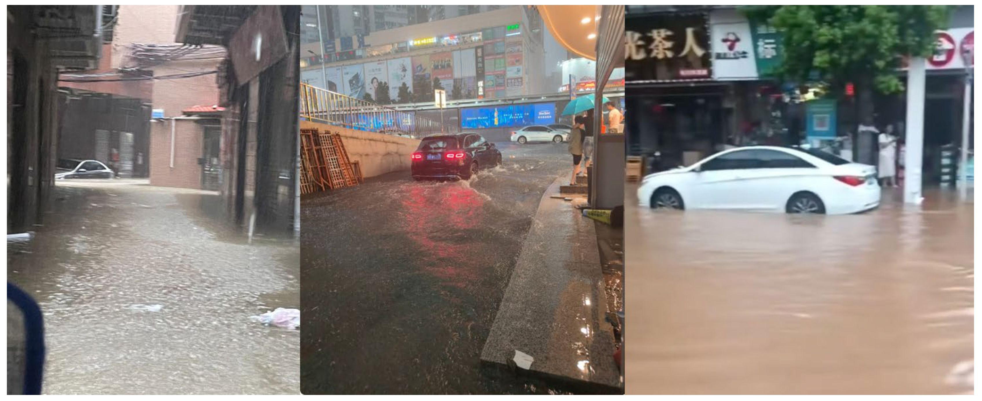
Figure 1. Some samples of urban floods in China (these photographs were taken in Shenzhen on 22 August 2024).
Sustainability 17 09973 g001
Figure 2. The study area: 6 representative cities in China.
Sustainability 17 09973 g002
Figure 3. The proposed methodology framework for constructing a mixed-city flood risk dataset. The data sources and their corresponding indicators are as follows: Sina Weibo (via Application Programming Interface, API); GPM (global precipitation measurement) for rainfall data; Zhongke Chaotu Geographic Data Cloud Platform for elevation data; and local statistical bureaus of various cities for building density and population density data.
Sustainability 17 09973 g003
Figure 4. Flood risk classification criteria based on water depth.
Sustainability 17 09973 g004
Figure 5. Overview of the mixed-city flood risk dataset. Population density is measured in persons per 30 m × 30 m (referring to the number of people within a 30 m × 30 m area); building density is measured in proportion per 30 m × 30 m (referring to the proportion of built-up area within a 30 m × 30 m area).
Sustainability 17 09973 g005
Figure 6. P-SGCN model architecture.
Sustainability 17 09973 g006
Figure 7. PSO-optimized SGCN framework.
Sustainability 17 09973 g007
Figure 8. Convergence curve of optimized SGCN with PSO.
Sustainability 17 09973 g008
Figure 9. Different models in six city test sets with true urban flood situations on map.
Sustainability 17 09973 g009
Figure 10. Confusion matrices depicting the performance of different models on our test set: (a) GCN; (b) LSTM; (c) P-SGCN.
Sustainability 17 09973 g010
Figure 11. Application and validation of different models in Dongguan.
Sustainability 17 09973 g011
Table 1. Collected data and sources.
DataResolutionYearSource
Urban floodPoint data2015–2024Sina Weibo
Precipitation0.1° × 0.1°2015–2024GPM [50]
DEM30 m × 30 m2015–2020Zhongke Chaotu Geographic Data Cloud Platform
Population Density30 m × 30 m2015–2020Local statistical bureaus of various cities
Building Density30 m × 30 m2015–2020
Table 2. The description of flood risk classification criteria based on water depth.
Risk LevelDescriptionWater Depth
d (cm)
Low risk
(0 level)
Incidents where no visible flooding is observed, or water submerges less than half of a car’s tire d   < 30
Medium risk
(1 level)
Incidents where water rises above the sidewalk curb or submerges half of a car’s wheel but does not reach the car’s engine hood30   d   < 50
High risk
(2 level)
Incidents where water submerges a car’s engine hood or reaches above pedestrians’ knees, potentially completely submerging vehicles d   > 50
Table 3. Optimizable parameters for PSO training in our SGCN model.
SGCN ComponentParameterTypeAnnotation
Graph dataset p g r a p h n IntNumber of nodes in the model’s input graph
p d FloatDistance-related coefficient
p h FloatElevation difference coefficient
p c i t y FloatCity relationship coefficient
GCN architecture p g c n n IntNumber of GCN layers
p g c n h i d IntNumber of hidden units in GCN
SNN architecture p s n n n IntNumber of SNN layers
p m IntNumber of neurons in the SNN
p T FloatTotal time for the simulation (SNN)
p t a u FloatDecay constant for synaptic current
p t a u s FloatTime constant for neuronal integration
Hyperparameters p e p o c h IntNumber of training epochs
p b a t c h IntBatch size for training
p l r FloatLearning rate for model training
Table 4. Optimized parameter results for PSO training in our SGCN model.
SGCN ComponentParameterOptimized ValueValue Range
Graph dataset p g r a p h n 52 to 10
p d 0.3340 to 10
p h 0.0160 to 10
p c i t y 0.0250 to 10
GCN architecture p g c n n 41 to 8
p g c n h i d 2058 to 256
SNN architecture p s n n n 31 to 8
p m 248 to 256
p T 1410 to 200
p t a u 232.7720 to 400
p t a u s 74.435 to 100
Hyperparameters p e p o c h 8720 to 200
p b a t c h 82 to 64
p l r 0.0351 × 10⁻⁵ to 1 × 10⁻¹
Table 5. Evaluation metrics for performance comparison of different models.
ModelPrecisionRecallF1 ScoreAccuracyPR-AUCROC-AUC
GCN0.72800.70840.71010.70840.74510.7623
LSTM0.63720.61470.61500.61410.65800.6752
P-SGCN0.84740.84560.84580.84560.87840.8921
Table 6. Sensitivity scores for different models and input features.
ModelPrecipitationPopulation DensityBuilding DensityElevation RelationshipProximity Relationship
GCN1.20.30.41.82.3
LSTM2.10.80.6N/AN/A
P-SGCN1.70.20.31.52.5
Table 7. Energy consumption and parameters of different models.
ModelParameters
(Million)
RAM Power
(kWh)
CPU Power
(kWh)
GPU Power
(kWh)
Total Energy
(J)
GCN2.065.4 × 10−69 × 10−65.4 × 10−653.5
LSTM2.371.8 × 10−61.8 × 10−62.7 × 10−620.4
P-SGCN1.313.6 × 10−69 × 10−69 × 10−611.9
Table 8. Performance of SGCN model transfer across individual cities (BJ: Beijing, SH: Shanghai, SZ: Shenzhen, HZ: Hangzhou, SJZ: Shijiazhuang, WH: Wuhan).
Model/DatasetBJSHSZHZSJZWH
Universal model0.8650.8530.8690.8090.8610.817
Universal model transfer to each city0.9040.8920.8700.8640.8610.878
Disclaimer/Publisher’s Note: The statements, opinions and data contained in all publications are solely those of the individual author(s) and contributor(s) and not of MDPI and/or the editor(s). MDPI and/or the editor(s) disclaim responsibility for any injury to people or property resulting from any ideas, methods, instructions or products referred to in the content.