Article

Panel Cointegration and Causality Among Socioeconomic Indicators in CEE Regions: Insights for Regional Economic Resilience and Sustainable Development

Faculty of Economic Cybernetics, Statistics and Informatics, Bucharest University of Economic Studies, Calea Dorobanți, 15–17, Sector 1, 010552 București, Romania
*
Author to whom correspondence should be addressed.
Sustainability 2025, 17(22), 9947; https://doi.org/10.3390/su17229947
Submission received: 5 August 2025 / Revised: 24 September 2025 / Accepted: 5 November 2025 / Published: 7 November 2025
(This article belongs to the Section Economic and Business Aspects of Sustainability)

Abstract

After the powerful socioeconomic shock of the fall of the communist regime in the early 90s, the ten countries in Central and Eastern Europe (CEE) analyzed in this study became growing Member States of the European Union (EU). However, they faced the 2008 financial crisis, the 2019 COVID shock, and sharp income disparities both at the regional level and compared to the countries in Western EU. This study explores the differences in sustainable regional development, modeling with Panel Autoregressive Distributed Lag (ARDL) to analyze relationships across multiple cross-sections in the short and long run, as well as with Cointegration Tests and Granger Panel Causality to detect evidence of causality among the variables in the study. The analysis covers 2012–2022, a period in which the Member States from CEE had the best access to generous structural and cohesion EU funds and that includes both the post-financial crisis convergence phase and the COVID-19 shock, enabling us to capture regional resilience dynamics. The results indicate that capital formation and population density positively influence disposable household income in the long run, across CEE regions, while unemployment and life expectancy exert negative effects. The results of this paper can be of use to decision-making institutions seeking to implement proactive socioeconomic policies in the lagging regions, before the next crisis, focused on capital investments, reducing unemployment, and bridging the rural–urban divide. The study contributes to the literature on inclusive and sustainable economic development at the CEE regional level.

1. Introduction

In today’s unpredictable world, disturbances such as epidemics, financial crises, wars, and natural disasters have increased in frequency, emphasizing the need to advance regional economic development and resilience. “Economic resilience” is the term describing a region’s capacity to adapt, adjust, and transform under certain shocks to its economic development [1], or from another perspective, it represents the ability to continuously create new paths for growth within the region [2]. The 2008 Great Recession attracted considerable attention from researchers attempting to investigate through the conceptual lens of resilience the causes that fueled the economic shock and its effects across countries and regions [3]. Some authors contributing to the literature on economic resilience have turned their attention to more recent global disturbances, such as the COVID-19 epidemic shock, supply chain crises, and wars [4]. In the flourishing literature, we find in studies different operationalization of the multifaceted resilience concept using GDP series, fluctuations in employment levels and other labor market indicators, economic performance and investment volumes, socio-demographic indicators, digital and innovation indicators, environment and urbanization, healthcare, or education measures [5,6,7,8,9]. The economic resilience literature follows a mixed structure of resistance concepts (how well the regional economy can absorb the shocks), recovery analysis (how fast the regional economy recovers from disturbances), re-orientation (how a regional economy can restructure itself after the shock), and renewal (to what extent a regional economy can create more suitable growth paths) [3].
High economic differentiation determines the difference in resilience across regions [10], which is why a relevant contribution to the progress of research on economic resilience is possible by shedding light on the socioeconomic regional inequalities. In the literature, the many faces of wealth inequality between countries and between regions have been frequently addressed [11]. In many European Union (EU) Member States, inequality has been on the rise in the past thirty years and has become more pronounced after the 2008 economic crisis [12]. In 2017, in the EU were existing two types of lagging regions: low-growth regions characterized by a persistent lack of growth, which did not converge to the EU average between 2000 and 2013, mainly located in the southern Member States, and the low-income regions, mainly eastern Member States, which remained much deviated from the EU average GDP per capita [13].
The differences in disposable income among EU countries are important, as highlighted in Figure 1. Countries shaded in yellow and light yellow (Luxembourg, Germany, Austria, Belgium, Netherlands) have a high and very high disposable income per capita, while countries shaded in orange and dark orange, which include all CEE countries, have a low (Czechia, Lithuania, Poland, Slovenia) and very low (Bulgaria, Estonia, Hungary, Latvia, Romania, Slovakia) disposable income per capita compared to the EU average.
In recent years, sustainability has become a central pillar of the EU’s policy, through European Green Deal and cohesion policy objectives. Regional economic disparities hinder social cohesion and represent an important obstacle to sustainable development. Structurally weak regions sometimes struggle to adapt to environmental, demographic, and technological transition. Economic resilience and social inclusion are linked to active participation in a process of sustainable development.
In the early 1990s, CEE countries had to adapt, adjust, and transform their economic systems toward market-based ones under the shock of the communist regime’s fall. These countries started a ‘post-socialist transformation process’ of their economies, with privatization steps and market reforms, while state-owned firms whose outputs were sold at prices determined by nonmarket mechanisms had to face major changes in the production model to offer competitive products in global markets [14]. Expectations were that privatization and liberalization of the economies would correct the imbalances accumulated from the communist regime, leading to prosperity for most people [15]. In the past three decades, CEE countries have gone through a major transformation from former communist countries to dynamically growing members of the EU. Different growth trajectories have been recorded in CEE countries during the transition period, the main explanatory factors for the differences being the time when the reforms were carried out, the speed of changing from a centrally planned economy to a market economy, and the macroeconomic policies implemented in the early years of the transition [16,17]. During the period 2000–2014, there are six CEE countries that recorded very high economic development dynamics: Romania (RO), followed by Slovakia (SK), Estonia (EE), Bulgaria (BG), Latvia (LT), and Lithuania (LV), and the economies of other four CEE countries, Czech Republic (CZ), Hungary (HU), Slovenia (SI), and Poland (PL), developed with a good GDP growth pace [10]. However, measured by the average value of GDP, CEE economies are relatively small in comparison to the economies of Germany (DE), France (FR), United Kingdom (UK), or Italy (IT). It is noteworthy that CEE regions occupy negligible places in world city rankings, from financial services and other specific indicators perspectives [18].
Even though the CEE regions, particularly the capital regions, have managed to support GDP growth over the last three decades, the success in improving living standards and achieving convergence towards equitable prosperity among the majority of the population has been limited [19]. CEE countries are characterized by sharp regional disparities. In these countries, there are major differences in development between urban regions and rural regions, between the main metropolitan region and the rest of the regions, and the western regions often perform better than their eastern regions [15]. Population in CEE countries is increasingly concentrated in a smaller number of prosperous regions, particularly the capital areas, in contrast to an increasing number of regions that are experiencing a decline in population density, hence the demographic development in CEE regions, further exacerbated problems of deepening regional inequalities in CEE countries [20]. Although the EU has adopted regional and cohesion policies in the past years, regional inequalities have increased [15].
Considering these aspects, this study investigates the long-run and short-run relationships among relevant socioeconomic indicators and regional disposable income levels in 56 NUTS2 regions from 10 CEE countries. The analysis aims to identify how structural factors such as investment (GFCF), unemployment (UNEMP), life expectancy (LIFEEXP), and population density (POP) contributed to disparities in disposable income (INC) during 2012–2022. Cointegration and a panel ARDL model are used to explore the mechanisms behind regional economic resilience and inequality in CEE context. Our findings provide a basis to formulate policies for regional development and convergence in the EU.
The study is guided by several research questions. First, we check whether a long-run equilibrium exists between INC and socioeconomic drivers in CEE. Second, we explore which of the variables GFCF, UNEMP, LIFEEXP, and POP affect INC in both the long and short term. Third, we evaluate to what extent these factors explain the persistent regional disparities observed across NUTS2 regions in CEE. To respond to these questions empirically, we test four hypotheses:
H1. 
GFCF has a positive long-run effect on INC, reflecting the role of capital investment in stimulating regional economic growth of lagging regions, these showing resilience when facing shocks.
H2. 
UNEMP has a negative long-run effect on INC, reflecting its detrimental influence on labor market participation and households’ living standards.
H3. 
LIFEEXP is negatively associated with INC in the long run, due to demographic aging and fiscal dependency pressures.
H4. 
POP contributes positively to INC in the long run, reflecting the productivity brought by urban agglomeration which, however, sharpens regional inequalities.
The paper is organized in five sections. The next section Section 2 contains a comprehensive literature review that contextualizes the socioeconomic transformation of CEE regions. Section 3 presents the data and the methodology. Section 4 contains the empirical results, first capturing the relationship between socioeconomic indicators of the CEE regions, then carrying out several regional comparisons. Section 5 ends the paper with conclusions and policy recommendations.

2. Literature Review

2.1. Socioeconomic Development Highlighting Regional Differentiation

A country’s economic development can be viewed as a continuous change in its socioeconomic life that enriches the living standards for its population [21]. The analysis of socioeconomic development is nourished by a variety of research topics, such as urban green spaces’ impact on socioeconomic variations [22], how cultural tourism or environmental sustainability signal socioeconomic development [23,24], disparities in social and economic development [25], and the role of structural change on resilience [26]. There is empirically based research claiming that less inequality benefits all, and that a more socially and spatially even society would produce more growth [27]. But the reality in Europe as well as in all other parts of the world indicates the existence of inequalities and their increase. European countries are characterized by regional polarization of the level of economic and social development, with the economically well-developed regions differentiated by the agglomeration of a highly specialized workforce, high GDP per capita, capital investments, and many financial, cultural, and research centers [28]. Inequality may relate to income and wealth and to different levels of socioeconomic development, but also to aspects related to education, basic services, or infrastructure [12].
In recent decades, economic inequality has deepened in many EU countries, and NUTS2 regions are heading towards a higher level of income inequality [29]. In 2017, in EU-28, the highest income disparities measured with Gini coefficient were recorded in Lithuania and Bulgaria (of over 35.0%). The report indicates countries having a Gini coefficient above the EU-28 average: Italy, Estonia, the United Kingdom, Romania, Greece, Portugal, Latvia, and Spain, as well as countries with less income disparity: Slovenia, Slovakia, the Czech Republic, Belgium, and Finland [12]. Carrera et al. [30] reported the evolution of regional inequalities for 22 EU countries, from 2000 to 2016. Authors found wider disparities on a regional level than on a country level, and an increasing disconnection between the distribution of production and the distribution of incomes. IT infrastructure, research and development expenditures, employment, and the number of universities increase regional GDP in the long term [31]. These findings reinforce the importance of innovation and human capital in driving regional convergence. R&D and digitalization act as main mechanisms for stimulating productivity and structural transformation across lagging regions.
Previous research has emphasized that inclusive growth, equitable access to capital and social welfare measured by life expectancy, and employment are drivers of sustainability. The capacity of a region to sustain economic activity and attract investment is connected to its socioeconomic structure. Convergence and cohesion policies are components of sustainable development.
Everywhere in Europe, the regional inequalities remain sharp in rural areas and the peripherally located former industrial areas, continually losing distance from more developed areas. For Great Britan (GB), for example, London metropolitan area is the leader in development, dominating economically over other GB areas [28]. The least developed GB regions are the peripherally located regions, in which tourism and agriculture play an important role. Referenced authors argue regional inequalities in GB are high and growing.

2.2. Regional Disparities in CEE Countries

Researching the multiple facets of regional disparities is relevant for CEE countries, as these countries have gone through a rapid exposure to processes of internationalization after the socioeconomic changes in the early 1990s and after their accession to the EU in 2004–2007 [15]. After belonging to the EU structures, all CEE countries benefited from EU supporting schemes like structural funds. In regions that have absorbed Cohesion Policy funds, the pace of reducing inequality has been faster, suggesting therefore that the structural funds alleviated socioeconomic disparities [29]. Still, after 2000, CEE countries experienced disproportionally high increases in regional disparities compared to the EU15 states [15,32,33].
Regarding CEE regional disparities, several studies have addressed the determinants of foreign direct investments and their positive spillovers on regional economies [34,35]. Others have given attention to the contribution of regional innovation systems to inequalities convergence [36]. Motivated by the highly uneven regional GDP growth rates observed within CEE countries, ref. [14] assessed the relationship between industrial restructuring and economic growth of CEE regions, focusing on a regional level analysis, covering 1995–2004 data. Results show that those regions that have succeeded in reconverting their production specialization to new sectors with higher value functions achieved better economic performance.
Ref. [37] focused on factors that determine cross-national variation in economic inequality trends in 10 CEE countries. Their results, found using random-effects regression models, emphasize that changes in income inequality in CEE countries in the first years after 1989 were influenced by the expansion of the private sector, penetration of foreign capital, retrenchment of the redistributive state, and the social exclusion of national minorities. Authors found that income disparities have risen faster in those CEE countries that privatized more substantially after 1989, or in those that received more capital investments per capita.
The leaders of the CEE countries in terms of bonding social capital are Estonia, Slovenia, and Poland, while people in Czech Republic and Slovenia are happiest [38].
Among others, ref. [39] signaled for CEE countries a strong socioeconomic spatial polarization between metropole regions and the remaining regions. Smolińska-Bryza et al. [40] shed light on the regional differences in Poland, one of the CEE countries, evaluating the inequalities in socioeconomic development between the NUTS2 regions in two time intervals, 2010–2012 and 2020–2022. In their study, authors note Poland’s accession to EU structures has triggered remarkable socioeconomic development through EU cohesion funds, particularly in the regions of the west of the country, contrasting with the pace of development in the eastern regions of the country. EU funding through the cohesion program aimed at reducing regional differences, but the authors note that the efficiency of reaching this goal varied. If in regions such as Mazowieckie and Dolno’slaskie, the improvements in socioeconomic development have been major, in other regions such as Lubusz or Warmian-Masurian, the improvements have been less important. Mazowieckie area, which includes Warsaw, the country’s capital city, is emphasized as being the most economically advanced area, having a high density of education and financial services, as well as a variety of employment opportunities [40].
Ref. [41] highlights the dual dynamics of cross-country convergence and within-country divergence in the EU. Ref. [42] document the impact of the COVID-19 crisis on regional inequalities across NUTS2 regions. Our paper advances the debate by applying panel ARDL, cointegration, and causality analysis to CEE regions over 2012–2022, thus capturing both short- and long-run dynamics and explicitly disentangling the effects of capital formation, unemployment, life expectancy, and population density on income disparities.
A comparison based on research objective, territory, time interval, and results for selected studies covering socioeconomic development in connection with regional disparities in European countries is provided in Table 1.

2.3. Research Gap

This analysis is carried out in two steps: in the first we capture the relationship between socioeconomic indicators of the CEE regions and their relevance in supporting both income inequalities convergence among regions and economic resilience, and in the second step we indicate major differences in development between urban core regions and rural regions in CEE. Comprehensive and dynamic analysis of how structural socioeconomic factors jointly affect disposable income, highlighting regional disparities and economic resilience insights, is not widely debated in the literature. Most studies focus on national data, ignoring long- and short-run dynamics, or overlooking cross-sectional dependence. This study fills the gap by using panel ARDL with cointegration and causality tests to explore how gross fixed capital formation, unemployment, life expectancy, and population density influence disposable household income across all CEE regions. The explanatory variables of the econometric models have been selected because each provides an essential and unique perspective in the socioeconomic landscape of a region: the potential for regional development (GCFC variable), the perspective of employment conditions and regional social stability (UNEMP variable), the health perspective of the population (LIFEEXP variable), and last but not least, the perspective of short-term recovery from a shock through a demographic mechanism (POP variable) [7,8,45,46,47].

3. Methodology

3.1. Cross-Sectional Dependence

Panel data models are widely used in economics and finance to analyze complex systems. They capture both differences and interdependencies across cross-sections. Cross-sectional dependence (CD) in panel data appears when observations across entities are not independent at some moment. This may result from common shocks (e.g., global crises, environmental changes, etc.), geographic proximity, or network effects [48].
In practice, CD means that a change affecting one cross-section may influence others, creating correlated errors. Ignoring CD leads to biased estimates or wrong conclusions. In this paper we test CD by means of the Breusch and Pagan Lagrange Multiplier (LM) [49], the Pesaran scaled LM test [50], and the Pesaran CD test [50]. The Pesaran tests were created for large panel data settings and improve the Breusch–Pagan LM test.

3.2. Panel Unit Root Tests

The data stationarity is tested by means of some panel unit root tests: Levin, Lin, and Chu (LLC) [51]; Im, Pesaran, and Shin (IPS) [52]; and the Augmented Dickey–Fuller test (ADF), by Maddala and Wu [53].
Panel unit root tests have the following formulation:
y i t = ρ i y i t 1 + z i t γ + u i t
In Equation (1), i = 1 , , N denotes the index for the unit (country); t = 1 , , T is the time (year); z i t is the deterministic term; and u i t is the error term. The null hypothesis NH is ρ i = 0 , for each i i. N is the number of units and T is the number of periods. is the first difference operator.

3.2.1. LLC Panel Unit Root Test

Levin et al. [51] assumes a common autoregressive coefficient across all individuals such that ρ i = ρ for all i . The NH is ρ i = ρ = 0 , indicating a unit root, while the alternative hypothesis AH is ρ i = ρ < 0 for all i. The LLC expression is
y i t = ρ i y i t 1 + α o i + α i t t + u i t ,   = 1 , , N ,   t = 1 , , T
Equation (2) has both a time trend component α i t t and individual specific effects.
u i t = j = 1 θ i j u i t j + ε i t
For panels with N between 10 and 250 and T between 25 and 250, LLC test is recommended [51]. A limitation of the LLC test is that it assumes identical autoregressive parameters across all units [54]. The NH is
NH :   ρ 1 = = ρ N = ρ = 0
Versus the AH:
AH :   ρ 1 = = ρ N = ρ < 0 .

3.2.2. IPS Panel Unit Root Test

IPS panel unit root test [52] uses the t-bar statistic, which allows for heterogeneity in the autoregressive parameter ρ i across individuals. Unlike the LLC test, the IPS test allows ρ i to vary across individuals. Its specification is
y i t = α 0 i + ρ i y i t 1 + j = 1 p i φ i j Δ i t j + ε i t ,   = 1 , , N ,   t = 1 , , T
The NH is ρ i = 0 , i = 1 , , N , meaning that all series have a unit root. The AH is ρ i < 0 , i = 1 , , N 1 ; ρ i = 0 , i = N 1 + 1 , , N . The t-bar statistic is
t ¯ = 1 N i = 1 N t i T
In Equation (5), t i T is the ADF test [53]. The IPS test performs effectively when both the cross-sectional dimension (N) and time dimension (T) are sufficiently large [52]. Simulation studies [55] suggest that the test has good size and power properties when N ≥ 10–20 and T ≥ 20–25. The test assumes that individual series are integrated of order one and that CD is weak; otherwise, results may be biased.
We acknowledge that with T = 11, the IPS test may suffer from size distortions. To mitigate this, we complement IPS with alternative panel unit root tests (e.g., Fisher–ADF) that are more robust in small-T contexts. By using Pedroni and Kao cointegration tests, which remain informative in small-T but large-N settings, we increase confidence in the robustness of our results. The use of the ARDL error-correction framework provides an additional check, since ARDL is well suited to small-sample panels and allows both short- and long-run dynamics to be estimated consistently.

3.2.3. ADF Panel Unit Root Test

Maddala and Wu [53] introduced the ADF–Fisher panel unit root test. This test aggregates p-values from individual ADF tests across cross-sections. It allows for heterogeneity in intercepts and lag structures. This makes it more flexible for testing panel data stationarity.

3.3. Panel Cointegration Tests

Cointegration tests assess evidence of a long-term causality. Cointegration tests consider both cross-sectional and time-series variation. Pedroni [56,57] introduced seven different statistics. These statistics verify the NH of no cointegration against the AH that at least one cointegrating relationship exists. The methodology distinguished between two groups:
Within-dimension tests (Panel statistics) assume common autoregressive coefficients across different panel members. Between-dimension tests (Group statistics) allow for individual autoregressive coefficients.
To account for potential CD, Pedroni [56] suggests adjusting the data by subtracting the average value from all unit at each period:
y ¯ t = 1 N i = 1 N y i t
The regressions used to generate the residuals for the test statistics are available in [56,58]. Further documentation on the methodological aspects is available in [56,59].
Kao panel cointegration test by Kao [60] is simpler. It assumes the same autoregressive coefficient for all cross-sections but allows different intercepts. Residuals from the cointegration equation are used and an ADF-type unit root test is applied. Kao [60] introduced a modified Dickey–Fuller t-test for checking cointegration. Both Kao and Pedroni tests can be applied if the variables are integrated of order 1, I(1), and help identifying long-term relationships in panel data.

3.4. Panel ARDL

The Panel ARDL (Autoregressive Distributed Lag) model extends the ARDL technique by Pesaran and Shin [61] to panel data. It is used to analyze relationships between variables across multiple cross-sections in short and long run. An advantage of the panel ARDL model is that it deals with variables that are stationary in level or in first difference. The ARDL model can be expressed as an Error Correction Model (ECM), which separates short-term dynamics from long-term equilibrium path. It permits heterogeneity across units.
The ARDL(p,q) model can be formulated in [61] as follows:
y = j = 1 p φ i j y i t j + j = 0 q δ i j x i t j + ϑ i + ϵ i t
In Equation (7), i = 1 , , N , t = 1 , , T , N is the number of units, T is the number of periods, ϑ i is the fixed effect of the cross-sections, and p and q are lag lengths. The Error Correction Term (ECT) describes the long-run equation of the ARDL model:
y i t = Φ i y i t 1 + θ i y i t + j = 1 p 1 φ i j Δ y y i t j + j = 0 q 1 δ i j Δ x i t j + ν i + ϵ i t
In Equation (8), Φ is the ECT, θ i is the long-run coefficient, and φ i j and δ i j are short-run coefficients. The ECT coefficient should be negative, in the interval [−1, 0], and statistically significant to confirm the presence of cointegration.

3.5. Granger Panel Causality Test

Granger causality by Granger [62] is a statistical hypothesis test used to determine if one time series can predict another. If a variable X Granger-causes another variable Y, then the past values of X provide information to forecast Y that is not contained in the past values of Y alone. The formulation of the Granger causality test assumes estimating two models.
The unrestricted model in relation (9) includes lagged values of both the dependent variable Y and the independent variable X. One assesses whether X provides additional predictive power for Y:
Y t = α 0 + i = 1 p α i Y t i + j = 1 q β j X t j + ε t
The restricted model in relation (10) includes lagged values of the dependent variable Y. It serves as a baseline to assess if excluding X reduces the model’s explanatory power:
Y t = γ 0 + i = 1 p γ i Y t i + u y
The NH H 0 is that X does not Granger-cause Y, which implies all β j = 0 . If the NH is rejected by means of an F-test or a Wald test, then X Granger-causes Y.
All empirical analyses were performed using RStudio 2023.12.1 and EViews 13.

4. Results

4.1. Input Data

We assemble a first dataset for the period 2012–2022, covering all 56 NUTS2 regions in the following ten CEE countries: Bulgaria (BG), Czech Republic (CZ), Estonia (EE), Hungary (HU), Latvia (LV), Lithuania (LT), Poland (PL), Romania (RO), Slovakia (SK), and Slovenia (SI), and a second dataset which covers in addition two out of four NUTS2 regions in Croatia (HR), for the time interval 2013–2022 (the other two NUTS2 regions in Croatia were not included because of data limitations). Other CEE countries were not included in our study because they are not EU Member States (Serbia, Bosnia and Herzegovina, Albania, Montenegro), thus they did not have the opportunity to absorb EU cohesion funds aimed at reducing income disparities. The disposable income of private households (INC) reflects the net resources, earned during the period, which are available for consumption and/or saving, adjusted to take account of social transfers in kind [63]. It expresses income disposability and captures disparities in income levels [64], being an important measure of residents’ living standards, so in the face of shocks, regions with higher living standards tend to have stronger resilience and faster recovery times [8]. Disposable income per household is one of the three indicators used to measure and report economic convergence in EU, along with GDP per capita and income inequality [65]. Gross fixed capital formation (GCFC) is key in compiling capital stocks data and balance sheets, covering mostly machinery, equipment, buildings, or other structures that are used repeatedly or continuously in production over periods of time of more than one year [45]. This indicator is used in studies as a measure of development potential [7]. Unemployment rates are one of the key indicators for evaluating employment conditions and social stability. When a region encounters sudden shocks, the higher the number of unemployed people, and the less stable society becomes [8]. Life expectancy (LIFEEXP) is frequently used as a summary indicator of population health [46,66]. Population density (POP) is a key social and economic indicator in short-term recovery after shocks [47]. Educational attainment (EDUC) plays a major role in the labor market, in the lives of individuals, and in society in general, with higher levels of education usually leading to higher rates of employment, higher productivity, and higher lifetime earnings for individuals [67]. Youth employment rate (YEMP) is an indicator capturing the engagement of young people in the labor market and society, their individual economic success, and their well-being [68]. Table 2 summarizes the research variables, source, and measurement units.
The analysis covers the period 2012–2022. This temporal span was chosen for several reasons. First, it captures the post-financial crisis convergence phase following the 2008–2010 recession, when CEE regions entered a more stable trajectory of socioeconomic adjustment. Second, the time frame covers the EU’s 2014–2020 Cohesion Policy program, during which CEE regions had access to important structural and cohesion funds aimed at reducing disparities, as well as the start of the 2021–2027 funding cycle. Third, it allows us to observe both the pre-COVID convergence dynamics and the impact of the COVID-19 shock (2019–2021), offering a meaningful test of regional resilience. By starting in 2012, we ensure comparability across CEE Member States that had full access to EU cohesion instruments, excluding those that joined the EU later or had delayed absorption capacity (e.g., Croatia, which joined the EU in 2013). Thus, the 2012–2022 interval aligns with critical turning points in regional development and EU policy cycles.
The violin plots in Figure 2 show the distribution of each variable across NUTS2 regions. Wider sections indicate a higher concentration of regions, while narrower sections suggest fewer. Symmetrical plots reflect even distributions, while asymmetry points to skewness. Peaks represent the most frequent values, and long tails represent outliers or broader spreads [69].
The violin plots point to structural disparities among CEE regions. The right-skewness in INC and UNEMP means that wealth and jobs are concentrated in metropolitan centers. Peripheral regions face long-term labor market issues [12,15,70]. POP is extremely uneven, implying that capital areas attract most economic activity, consistent with demographic polarization between urban hubs and rural regions [14,20]. GFCF and EDUC are also skewed, showing that investments and higher education opportunities cluster in more developed regions [29,31]. By contrast, LIFEEXP appears more evenly distributed, pointing to the equal role of national healthcare policies among regions [46,66].
One can notice important disparities in development, living standards, and labor market dynamics of the socioeconomic indicators during 2012–2022. INC and UNEMP distributions are right skewed. Most NUTS2 regions have disposable incomes between 15,000 and 25,000 units and low unemployment (around 4–6%), while a few have INC values exceeding 60,000 units, and some regions reach unemployment rates over 15%. It means that household wealth is concentrated in a small number of regions, e.g., economically advanced areas, revealing a broader income inequality across the CEE regions. Employment conditions are generally stable, but some NUTS2 regions face structural labor market issues due to industrial decline, low educational attainment, or weak economic diversification. POP distribution shows extreme right skewness. The majority of CEE regions have moderate population density, with values below 500 units, while a few show very high density, above 3000 units, indicative of large urban centers. This points to the fact that POP distribution is spatially dispersed, urbanization and economic activities being highly concentrated in a few main regions. GFCF is highly skewed to the right. Most NUTS2 regions cluster at the lower end of the spectrum, below 10,000 units, with only a few outlier regions showing importantly higher investment levels. These outliers correspond to regions with major development potential, industrial zones, or metropolitan areas where capital-intensive projects are more common. The disparity implies an unequal distribution of economic development and capital stocks across NUTS2 regions. The violin plot of EDUC shows a moderately right-skewed distribution. Even if most regions in CEE countries have between 20% and 35% of their population attaining tertiary education, some regions reach above 45%. It signals that educational resources or opportunities are concentrated in more developed areas. This uneven distribution points to regional gaps in access to or quality of higher education. LIFEEXP distribution is narrow and symmetric, with values ranging between 74 and 78 years, signaling that population health level across CEE NUTS2 regions is relatively consistent, due to national healthcare policies. Local socioeconomic conditions or healthcare access might produce lower variations. YEMP distribution is left skewed. Most NUTS2 regions report high levels of youth employment, often above 70%. This reflects that young people are effectively integrated into the workforce in most areas. At the lower end, we identify several NUTS2 regions needing targeted support to improve opportunities for young adults, especially in terms of education-to-employment issues.
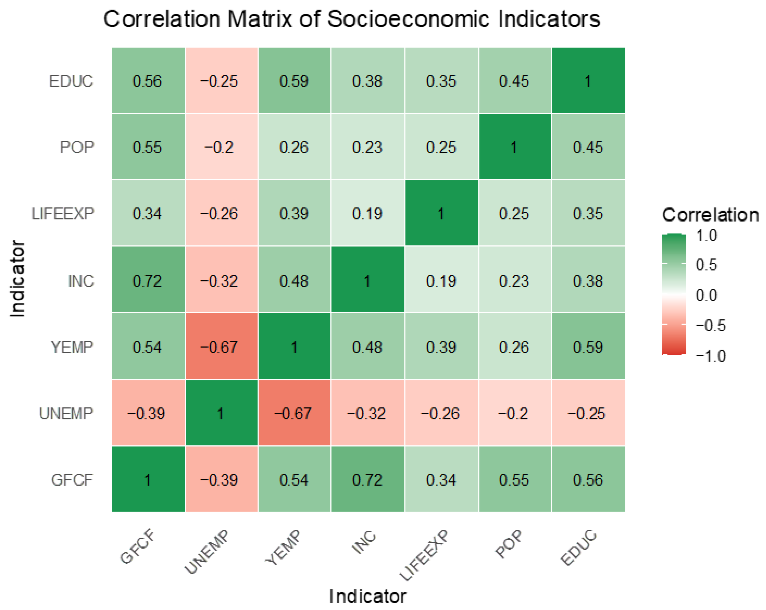
The correlation matrix in Figure 3 reports the relationships among the selected socioeconomic indicators across CEE regions for the period 2012 to 2022. The heatmap points to moderate and weak correlations among the variables, with both expected and policy-relevant patterns. All correlation coefficients fall below 0.8. There is no indication of severe multicollinearity that would distort further ARDL regression results.
GFCF and INC have the strongest positive association, with a correlation of 0.72. This suggests that NUTS2 regions with higher levels of investment activity also report higher household disposable income. This reflects the mutually reinforcing relation between capital accumulation, productivity, and income generation. GFCF also shows moderate positive correlations with YEMP (0.54), POP (0.55), and EDUC (0.56). It follows that capital-intensive regions are often more urbanized, have higher levels of education, and offer better employment prospects for young people.
EDUC is moderately correlated with several indicators, YEMP (0.59), INC (0.38), and LIFEEXP (0.35). These correlations point to the benefits of education in improving health level and labor market integration. YEMP is also moderately correlated with INC (0.48) and LIFEEXP (0.39) and negatively correlated with UNEMP (−0.67). NUTS2 regions with stronger labor market conditions for young people are usually more economically and socially developed.
UNEMP is negatively associated the other indicators in the correlation matrix in Figure 2. The strongest negative correlation is with YEMP (−0.67). UNEMP also has a moderate negative association with INC (−0.32), LIFEEXP (−0.26), and EDUC (−0.25). High unemployment rates characterize less developed regions, where income and human capital are also lower.
POP shows weak to moderate positive correlations with GFCF (0.55), INC (0.23), and EDUC (0.45). This implies that more densely populated regions are centers of economic activity and education.
The selected variables do not exhibit the degree of statistical dependency that would cause multicollinearity concerns in the panel ARDL model. Multicollinearity usually occurs when variables are highly correlated, i.e., r > 0.8 or VIF > 5 [71], as it inflates the standard errors of regression coefficients and leads to instability in parameter estimation.
The descriptive statistics of the socioeconomic indicators for the period 2012–2022 are contained in Table 3.
EDUC mean is 26.1%, and its values range from 11.2% to 62.1%. EDUC distribution is right skewed and leptokurtic. The standard deviation of 9.88 reflects moderate variability.
UNEMP has a mean of 6.18%, with a minimum of 1.2% and a maximum of 18.4%. UNEMP skewness and kurtosis suggest a moderately right-skewed and slightly peaked distribution. Most CEE regions have relatively low unemployment, but a few outliers have much higher levels.
YEMP has a mean of 74.6% and a symmetrical distribution. Relatively high mean and median values indicate a strong labor market inclusion of young people in most regions, even if a standard deviation of 7.06 points to some regional variation.
LIFEEXP is distributed around a mean of 76.57 years, with minimum and maximum values of 69.5 and 82.8, respectively. The near-zero skewness and kurtosis 3.35 confirm that the data is approximately normally distributed.
POP displays a significant dispersion, with a mean of 238.06 inhabitants per km2 and a very wide range from 29.7 to 3448.1. The right-skewed and peaked POP distribution indicates the presence of few very densely populated urban regions surrounded by many more sparsely populated areas.
GFCF has a mean of 4840.76 and a very large variation. POP distribution is right skewed and leptokurtic. This suggests the presence of a few highly investment-intensive regions among many that invest at more modest levels.
INC has a wide spread, indicating a skewed distribution. The skewness value of 1.89 and kurtosis of 7.15 confirm a right-skewed and fat-tailed distribution, with a few high-income CEE regions lifting the overall mean.

4.2. Empirical Results

The relation among the variables has the following form:
I N C = f G F C F ,   U N E M P , L I F E E X P ,   P O P
Even if EDUC and YEMP were part of the broader analysis to depict the regional development dynamics, they were excluded from the ARDL model due to model parsimony. Their effects on INC are captured indirectly, through included variables CGFC, UNEMP, LIFEEXP, and POP, which reflect labor market conditions, capital availability, and demographic structure.
Panel data modeling is used to deal with this case study. There are several advantages of panel data over cross-sectional or time-series data [72]: parameter stability, the ability to deal with hidden variables, reduced estimate bias, analyzing individual and group behaviors, etc.
First, we perform several CD tests: the Breusch and Pagan Lagrange Multiplier (LM) test [49], the Pesaran scaled LM test [50], and the Pesaran CD test [50]. We reject the hypothesis of no CD, as shown in Table 4. The econometric modeling that we further use assumes the presence of CD.
To verify the validity of long-term relationships among variables, in Table 5 we tested for stationarity using panel unit root tests: LLC, IPS, and ADF tests. After taking first differences, all variables become stationary at 1% significance level. This confirms the first-order integration, I(1). The condition is required for applying panel cointegration techniques to explore long-term relationships.
Since all variables are integrated of order 1, I(1), panel cointegration tests were performed by means of the Pedroni [56] and Kao [60] tests to verify whether a stable long-run relationship exists among the socioeconomic indicators. Table 6 reports the results of these tests. Several within-dimension statistics from the Pedroni test, namely the panel PP-statistic and the panel ADF-statistic, are significant, as are the between-dimension statistics, namely the group PP-statistic and group ADF-statistic. These results reject the NH of no cointegration at conventional significance levels. Six out of eleven tests indicate evidence of cointegration.
The Kao residual-based test in Table 7 also indicates cointegration, with a significant t-statistic (p < 0.01). Both the Pedroni and Kao cointegration tests prove that INC, GCFC, UNEMP, POP, and LIFEEXP share a common long-term equilibrium path across the NUTS2 regions.
The optimal model is ARDL (1,1,1,1,1). The ARDL (1,1,1,1,1) specification was chosen because including more than 1 lag would reduce the degrees of freedom and compromise model reliability. One lag was the maximum feasible lag number for all variables.
Table 8 contains the long-run and short-run estimated ARDL coefficients.
A one-unit increase in GFCF leads to a long-term increase of 1.31 units in INC. This indicates that greater capital investment corresponds to household disposable income growth. Regional economic resilience is enhanced by capital accumulation. Productivity increase and job creation are stimulated by investments in infrastructure and technology. This leads to higher wages and more household consumption. Hypothesis H1 is confirmed in this case. This finding aligns with Rodríguez-Pose and Crescenzi [73] who proved that investment in physical capital drives regional growth by means of knowledge spillovers in a study on EU-25 countries.
GFCF also generates multiplier effects. Better infrastructure generates lower transportation costs and facilitates access to markets. Private investments are attracted, and economic activity is boosted. The demand for labor increases and income growth is stimulated in urban and peripheral areas.
A one-percentage-point increase in UNEMP leads to a long-term decrease of 755 units in INC, confirming hypothesis H2. More UNEMP means that fewer people earn wages. Consumption and tax revenues decrease and reliance on social support increases. Broader economic spillovers of UNEMP include reduced investment activity and a slowdown in regional economic output. This result is consistent with Di Caro [70], who shows that regional resilience in Italy is caused by uneven responses to employment shocks. Areas with stronger industrial activity show greater resistance to crises, emphasizing the role of labor markets in sustaining local economic growth.
A one-year increase in LIFEEXP results in a long-term reduction of 1118 units in INC, validating hypothesis H3. Aging is associated with demographic and fiscal pressures. Living longer changes the population structure, such that the number of retired people increases and workforce reduces. The pension system can be under pressure during this demographic transition. Economic activity slows down, since old people save more and spend less. In regions with more elderly people, tax bases shrink and productivity decreases. The negative association between LIFEEXP and INC proves the existence of regional disparities. Longer LIFEEXP might be concentrated in less economically dynamic regions, where economic opportunities have stagnated. Although the impact of LIFEEXP on growth may be modest, in post-transition economies with weaker institutional capacity and less flexible labor markets, this influence is higher [74].
A one-unit increase in POP contributes to a rise of 1289 units in INC, proving hypothesis H4. This suggests that densely populated urban areas offer better income opportunities, sharpening regional inequalities. The agglomeration effect in urban regions raises productivity, wages, and access to services. These densely populated urban regions attract private investments and high-paying jobs. Similar long-run effects are observed in another study [75], where regional decentralization, disparities, and the distinct features of Romania’s macro-regions are examined.
Also, Brülhart and Sbergami [76] prove that spatial agglomeration stimulates economic growth in countries below a certain income level, particularly in lower- to middle-income countries like those in CEE.
In the short run, most explanatory variables do not affect INC. Immediate response to economic and demographic shifts is limited. The only exception is LIFEEXP, where a one-year increase in LIFEEXP leads to a rise of 196 units in INC. Better population health may be associated with higher productivity or lower health expenditures. GFCF, UNEMP, and POP do not affect INC in the short term. Their effect on INC emerges over time. Structural factors like capital formation and urban expansion manifest themselves in the long run.
ECT is negative and significant, belonging to [−1, 0]. This confirms a stable long-run relationship between INC and its determinants: GFCF, UNEMP, LIFEEXP, and POP. A total of 13% of any short-time deviations in INC is corrected annually. The speed of adjustment to long-run equilibrium after economic shock is moderate in this case.
As a sensitivity analysis of findings, Appendix A includes additional results obtained by including two Croatian NUTS2 regions, which allows us to assess the stability of the results relative to the baseline dataset.
Table 9 presents the bidirectional causalities among the variables.
There exists a bidirectional causality between GCFC and INC. Higher capital investment increases household disposable income by job creation and productivity. Conversely, a higher INC is associated with higher demand and savings, stimulating investments.
The bidirectional causality between INC and UNEMP indicates that less unemployment improves income. Conversely, the labor market gets more stable since higher income raises consumption and investment.
A bidirectional causality exists between INC and LIFEEXP. Healthier, longer-living populations correspond to higher productivity and income. Conversely, higher income improves access to healthcare and living conditions, leading to longer LIFEEXP.
The causal relationship from GFCF to LIFEEXP suggests that investment in infrastructure, healthcare, and public goods improves health conditions. The converse relationship indicates that a healthier population supports long-term economic activity and attracts more investment.
GFCF and POP are also in a bidirectional relationship. Population growth and density attract capital investment through agglomeration economies. Investment promotes urbanization by improving infrastructure and creating jobs.
LIFEEXP and UNEMP are mutually linked as well. Reduced healthcare access decreases labor force participation and increases unemployment. Weak labor markets worsen health outcomes, conversely.
No significant causality exists between POP and INC or between POP and UNEMP or LIFEEXP. It means that population growth alone does not lead to higher INC, better population health, or lower UNEMP. Targeted investments and supportive policies are needed to make population growth effective.
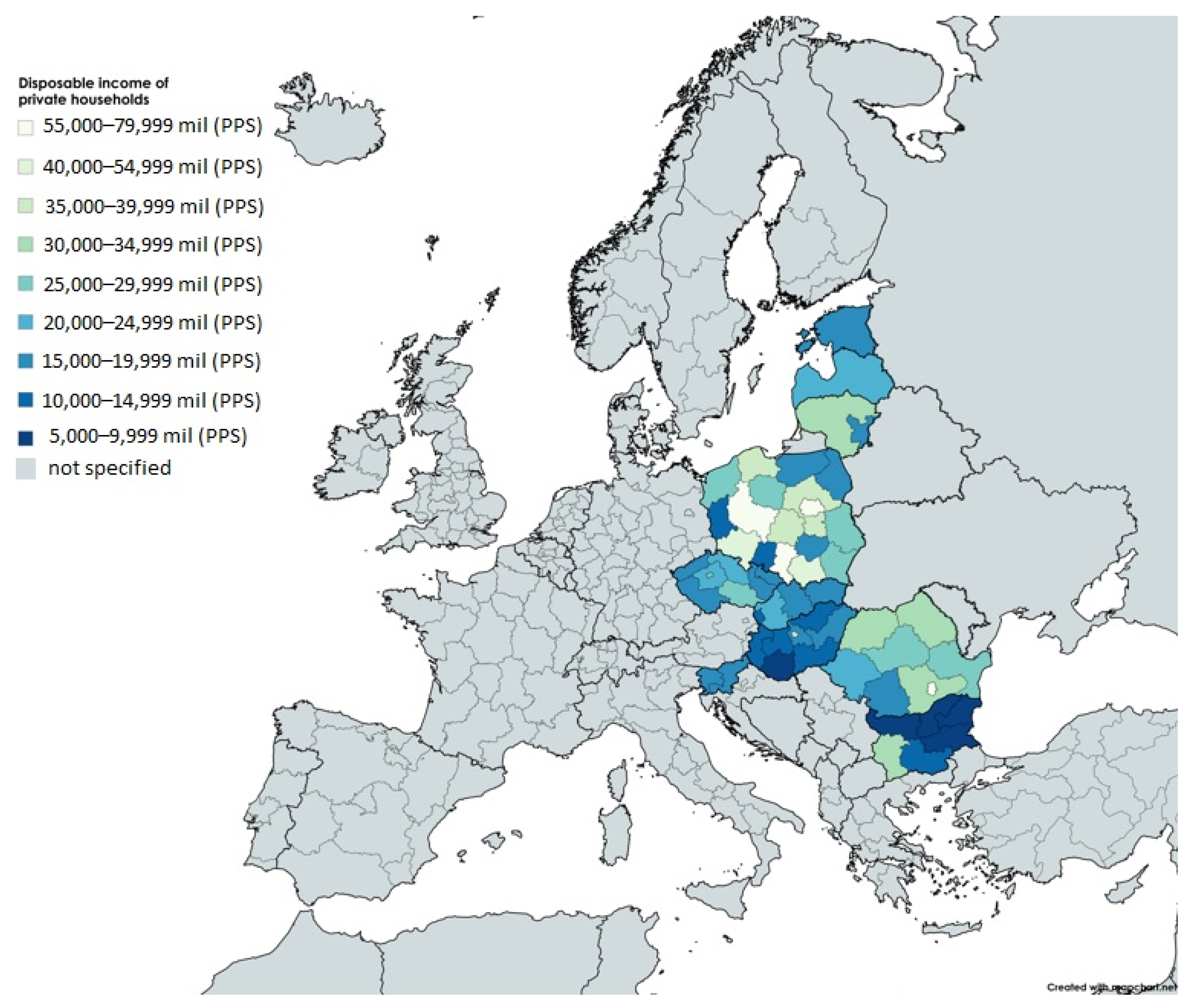
Sharp regional disparities are present in CEE, and Figure 4 allows visualization of them. For all CEE countries, the color palette is observed at the regional level, ranging from light green, indicating a region with a disposable income level of over 55,000 units, to a darker shade of green and up to an intense shade of blue, signaling a region with the lowest disposable income level.
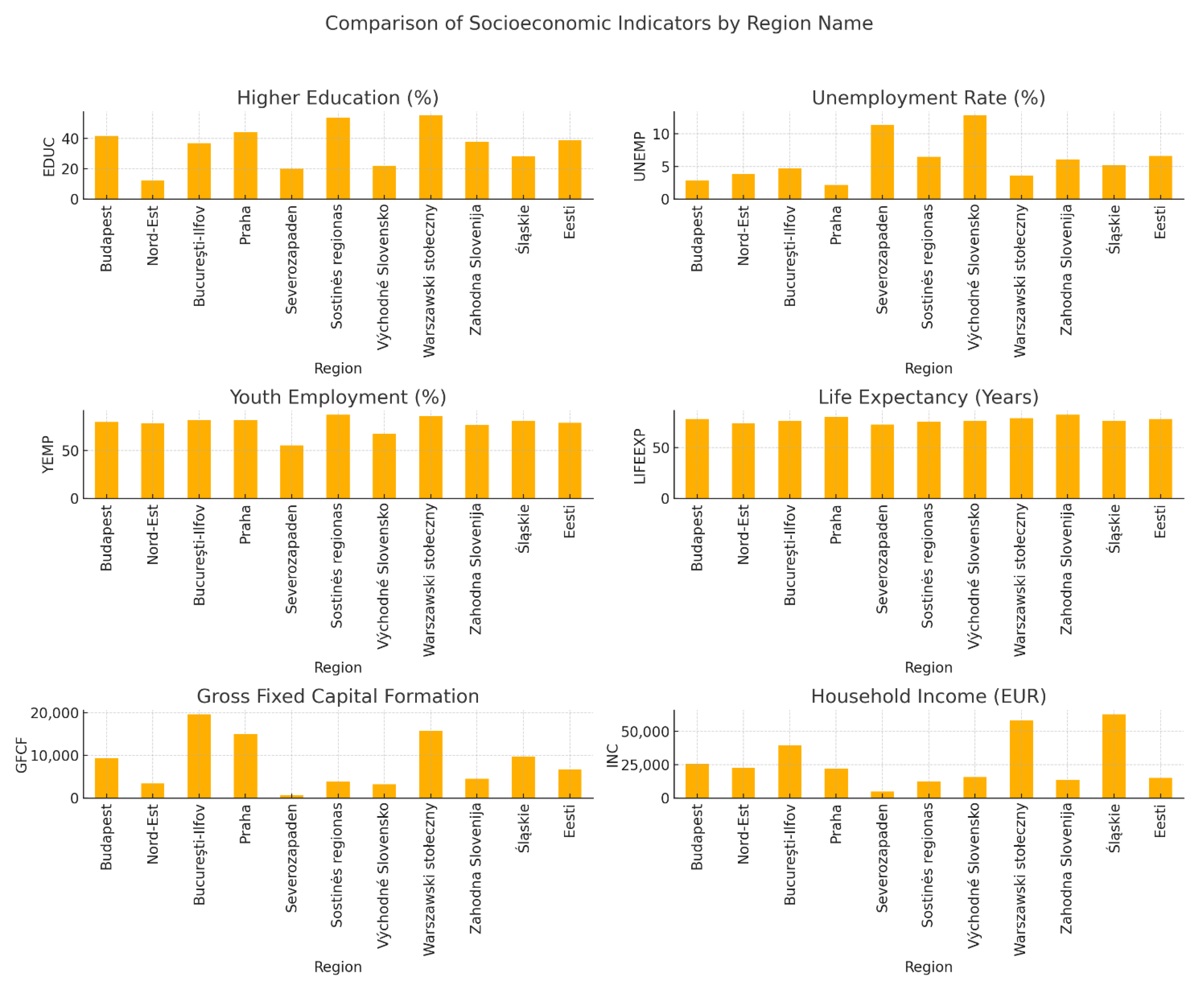
Figure 5 compares eleven selected regions using the mean values of the socioeconomic indicators. This regional comparison illustrates the spatial polarization of development in CEE, which further determines the difference in economic resilience across regions.
The selected NUTS2 regions include both capital areas—such as București-Ilfov (Romania), Budapest (Hungary), Praha (Czechia), Warszawski stołeczny (Poland), Sostinės regionas (Lithuania), and Bratislavský kraj (Slovakia)—and structurally weaker peripheral regions like Severozapaden (Bulgaria), Nord-Est (Romania), and Východné Slovensko (Slovakia). Through this selection of regions, we aim to carry out a comparative analysis of regional disparities in CEE countries.
Capital regions show high levels of socioeconomic development, being hubs of investment, innovation and national economic growth. București-Ilfov, Budapest, and Praha stand out as regions with high INC, GFCF levels and a strong youth market integration. Romania’s main economic hub is Bucuresti-Ilfov, leader in GCFC and INC. Budapest is characterized by high levels of education, strong labor market indicators, and a dense urban infrastructure. Praha has the highest LIFEEXP and the lowest UNEMP among the analyzed regions, with a social stable population and a diversified economy.
Other capital-adjacent regions such as Warszawski stołeczny, Sostinės regionas, and Bratislavský kraj also perform well across multiple indicators. Warszawski stołeczny is characterized by high income and employment levels. Sostinės regionas, which includes Vilnius, has moderate capital accumulation and disposable income levels, but performs strongly in life expectancy and education. Bratislavský kraj is characterized by a high educational attainment with good labor and investment indicators, aligning closely with Western European standards.
Peripheral rural regions such as Severozapaden, Nord-Est, and Východné Slovensko reveal persistent structural disadvantages. Severozapaden is a region in northwestern Bulgaria, one of the poorest in EU both in terms of GDP per capita and other socioeconomic indicators. Its ranking in last reflects long-standing issues such as weak infrastructure investments, limited access to education, and demographic decline. Nord-Est in Romania also exhibits low education levels and limited GFCF, even if it registers moderate YEMP and relatively low UNEMP. Východné Slovensko is less developed compared to western parts of Slovakia. This region faces higher UNEMP, lower INC, and less capital formation compared to Slovakia’s capital region.
Intermediate performers are Śląskie, Zahodna Slovenija, and Eesti. They have a balanced profile. Śląskie is a traditional industrial region in southern Poland with moderate income and investment levels, struggling to adapt its labor force to the requirements of post-industrial transformation. Zahodna Slovenija is located in the proximity of Italy and the Adriatic, with moderate GFCF and INC levels. Eesti, representing Estonia as a whole, shows high levels of population health, education, and employment, reflecting the benefits of sustained digitalization and institutional reforms. Estonia is often viewed as a digital front-runner and a model for e-governance and public sector innovation [77].

5. Conclusions and Policy Implications

The paper evaluated the relationship between five socioeconomic indicators of the CEE regions and identified the factors related to disparities in disposable income, providing insights into the differences in regional economic resilience in Central and Eastern Europe. The results confirm a long-run equilibrium relationship between disposable income, gross fixed capital formation, unemployment, life expectancy, and population density. Furthermore, these results allow us to return to the research questions set in the Introduction. Capital formation and population density have positive long-term effects on disposable income (H1 and H4 supported), reflecting the role of development potential and urban agglomerations in income regional convergence, while unemployment and life expectancy exert negative impacts (H2 and H3 supported), highlighting the importance of diminishing labor market weaknesses and demographic pressures to converge towards regions with small differences in income and economic resilience between them.
Given that the resilient aspect of a region can be measured if we consider the evolution of certain variables over a long run [6], we addressed in the analysis the long-run determinants of regional disposable income disparities and economic resilience across NUTS2 regions in CEE. The ECT coefficient confirming the presence of cointegration proved a stable long-run relationship between disposable income and its determinants, gross fixed capital formation, unemployment, life expectancy, and population density. The slow adjustment mechanism (ECT ≈ −0.12) suggests the persistence of regional disposable income and economic resilience disparities, as well as a structural rigidity that characterizes the convergence process in CEE.
The results of our paper point to the idea that there are regional disparities in socioeconomic indicators, hence different contexts to reacting to an economic or epidemic crisis: capital regions show highest levels of socioeconomic development, capital-adjacent regions also perform well across multiple indicators, intermediate performing regions have a balanced profile in terms of socioeconomic development, and peripheral rural regions reveal persistent structural disadvantages, being the least equipped to face the crises.
In terms of disposable income per household inequality, the convergence process among EU Member States was disrupted during 2011–2014 by the financial crisis, when there was a period of downward divergence, after which the EU returned to the path of improving indicators and convergence [65]. After a few years, in 2019, the process of convergence since 2014 was reversed by the impact of COVID-19 shock, and between 2019 and 2021, there has been increasing performance coupled with increasing disparities [63]. In this context of observing the increase in income disparities following a shock, as was observed after the 2008 Great Recession or after the COVID-19 shock, this paper discusses the need for EU-level policies to prevent the rise in income inequalities between regions in the period following the shock. A proactive attitude on the part of decision-making institutions is essential to intelligently manage the next shock. In the case of our research, based on the panel ARDL model with cointegration analysis results, the recommended preventive policy is a mix of measures in the lagging regions, focused on (1) capital investments; (2) reducing unemployment; and (3) bridging the rural–urban divide.
Our paper has several limitations, which include the short time span and restricted data availability, which constrain model robustness and variable coverage. Future research should expand the dataset with indicators regarding the funding absorbed by regions through the EU-funded regional cohesion programs, employment-to-population ratios, and structural change indicators (e.g., declining manufacturing, rising services) to allow a broader analysis of the socioeconomic indicators and trends among women, the elderly, and minority groups that are determinants for sustainable development, strengthening economic resilience, and reducing income inequalities between regions, with a view to specific funding programs, industry structural change, and labor market participation. Future research may incorporate NUTS 2 regions in Croatia, Serbia, Bosnia and Herzegovina, Albania, and Montenegro once consistent data are available, to enable broader and more robust cross-country comparisons within the CEE region. The application of spatial econometrics, or nonlinear ARDL models could capture heterogeneous effects of the regions and explain cross-sectional dependence.

Author Contributions

Conceptualization, M.B. and I.G.; methodology, I.G.; software, I.G.; validation, M.B. and I.G.; formal analysis, M.B. and I.G.; investigation, M.B. and I.G.; resources, M.B. and I.G.; data curation, M.B.; writing—original draft preparation, M.B. and I.G.; writing—review and editing, M.B. and I.G.; visualization, M.B. and I.G.; supervision, M.B. and I.G.; project administration, I.G.; funding acquisition, I.G. All authors have read and agreed to the published version of the manuscript.

Funding

This research received no funding.

Institutional Review Board Statement

Not applicable.

Informed Consent Statement

Not applicable.

Data Availability Statement

Data will be available on request.

Conflicts of Interest

The authors declare that there are no conflicts of interest.

Appendix A

We extended the dataset to include the two Croatian NUTS2 regions, Panonska Hrvatska and Jadranska Hrvatska, for which data were available, for the period 2013–2022. The ARDL (1,1,1,1,1) model was re-estimated with these additional cross-sections.
Table A1 confirms that the inclusion of the Croatian NUTS2 regions does not alter the integration properties of the variables. INC and GFCF are found to be integrated of order one, I(1), while UNEMP, LIFEEXP, and POP are I(0). Thus, the econometric requirements for estimating the ARDL model are maintained.
Table A1. Panel unit root tests (NUTS2 level, including Croatia).
At Levels
INCGCFCUNEMPLIFEEXPPOP
Unit root (Common Unit Root Process)
LLC13.17
(0.99)
5.88
(0.99)
−19.48
(0.000) *
−31.19
(0.000) *
−548.41
(0.000) *
Unit root (Individual Unit Root Process)
IPS14.81
(0.99)
7.83
(0.99)
−6.09
(0.000) *
−14.96
(0.000) *
−741.02
(0.000) *
ADF-Fisher Chi-square3.19
(0.99)
57.39
(0.999)
230.75
(0.000) *
257.99
(0.000) *
72.52
(0.000) *
At first difference
Unit root (Common Unit Root Process)
LLC−6.51
(0.000) *
−20.31
(0.000) *
−4.26
(0.000) *
−61.77
(0.000) *
−2598.32
(0.000) *
Unit root (Individual Unit Root Process)
IPS−3.80
(0.000) *
−7.69
(0.000) **
−1.87
(0.030) **
−21.44
(0.000) *
−809.26
(0.000) *
ADF-Fisher Chi-square188.64
(0.000) *
285.13
(0.000) *
137.65
(0.083) *
348.21
(0.000) *
165.329
(0.000) *
*, ** significant at 1%, and 5% level.
Table A2 reports the panel ARDL (1,1,1,1,1) estimates including the two Croatian NUTS2 regions. When comparing Table A2 with Table 8, the main hypotheses on GFCF and UNEMP (H1, H2) remain robust. GFCF continues to exert a strong positive effect on income, while UNEMP exerts a negative effect, though of smaller magnitude in the absolute value. However, the results for LIFEEXP and POP (H3, H4) are less stable. With the addition of Croatia, LIFEEXP turns positive and significant, suggesting that longevity supports INC in the enlarged sample. POP becomes negative and only weakly significant. The ECT loses significance, pointing to a weaker adjustment mechanism compared to the long-run equilibrium. The conclusion of the sensitivity analysis is that the main drivers of INC remain consistent, but demographic variables are more sensitive to sample composition.
Table A2. Panel ARDL (1,1,1,1,1) (NUTS2 level, including Croatia).
VariableCoefficientStd. Errort-StatisticProb. *
Long-Run Equation
GFCF2.830.2013.990.000 *
UNEMP−213.9935.83−5.970.000 *
LIFEEXP112.2410.5210.660.000 *
POP−6.723.23−2.070.038 **
Short-Run Equation
COINTEQ01−0.010.02−0.460.638
D(GFCF)0.390.113.350.000 *
D(UNEMP)−213.3357.35−1.970.048 **
D(LIFEEXP)43.1579.920.530.589
D(POP)−227.97173.01−1.310.188
*, ** significant at 1%, and 5% level.

References

  1. Davies, S. Regional resilience in the 2008–2010 downturn: Comparative evidence from European countries. Camb. J. Reg. Econ. Soc. 2011, 4, 369–382. [Google Scholar] [CrossRef]
  2. Boschma, R. Towards an evolutionary perspective on regional resilience. Reg. Stud. 2015, 49, 733–751. [Google Scholar] [CrossRef]
  3. Prodi, E.; Ghinoi, S.; Rubini, L.; Silvestri, F. Do informal institutions matter for the economic resilience of European regions? A study of the post-2008 shock. Econ. Polit. 2023, 40, 189–223. [Google Scholar] [CrossRef]
  4. Mantas, R.; Mindaugas, B. From adversity to advantage: A systematic literature review on regional economic resilience. Urb. Sci. 2025, 9, 118. [Google Scholar]
  5. Cellini, R.; Di Caro, P.; Torrisi, G. Regional resilience in Italy: Do employment and income tell the same story? In Handbook of Regions and Competitiveness; MPRA Paper No. 59660; University Library of Munich: Munich, Germany, 2014. [Google Scholar]
  6. Nijkamp, P.; Ţigănaşu, R.; Bănică, A.; Pascariu, G.C. Institutional adaptability: Its relevance for enhancing resilience and smart specialization capacity of the European Union’s lagging regions. Eurasian Geogr. Econ. 2022, 65, 1–33. [Google Scholar] [CrossRef]
  7. Peng, A. Sustainable regional development from the perspective of economic resilience: Based on the impact of COVID-19. PLoS ONE 2025, 20, 0314663. [Google Scholar] [CrossRef] [PubMed]
  8. Tian, S.; He, Y. The impact of digital industry development on regional economic resilience: Evidence from China. PLoS ONE 2025, 20, 0315203. [Google Scholar] [CrossRef]
  9. Gu, J.; Liu, Z. A study of the coupling between the digital economy and regional economic resilience: Evidence from China. PLoS ONE 2024, 19, 0296890. [Google Scholar] [CrossRef]
  10. Drobniak, A. Economic resilience and hybridization of development—A case of the central European regions. Reg. Stat. 2017, 7, 43–62. [Google Scholar] [CrossRef]
  11. Goldin, I. Why Do Some Countries Develop and Others Not? In Development in Turbulent Times: The Many Faces of Inequality Within Europe, 1st ed.; Dobrescu, P., Ed.; Springer: Berlin/Heidelberg, Germany, 2019; pp. 13–30. [Google Scholar]
  12. European Parliament. Regional Inequalities in the EU. Briefing 2019. Available online: https://www.europarl.europa.eu/RegData/etudes/BRIE/2019/637951/EPRS_BRI(2019)637951_EN.pdf (accessed on 19 May 2025).
  13. European Commission. Competitiveness in Low-Income and Low-Growth Regions. The Lagging Regions Report. 2017. Available online: https://ec.europa.eu/regional_policy/sources/studies/lagging_regions%20report_en.pdf (accessed on 19 May 2025).
  14. Capello, R.; Perucca, G. Industrial restructuring in CEE regions: Determinants of regional growth in the accession and in the crisis period. J. Balt. Stud. 2016, 48, 309–329. [Google Scholar] [CrossRef]
  15. Lang, T. Socio-economic and political responses to regional polarisation and socio-spatial peripheralisation in central and eastern Europe: A research agenda. Hung. Geogr. Bull. 2015, 64, 171–185. [Google Scholar] [CrossRef]
  16. Tichit, A. The Optimal Speed of Transition Revisited. Eur. J. Political Econ. 2006, 22, 349–369. [Google Scholar] [CrossRef]
  17. Svejnar, J. Transition Economies: Performance and Challenges. J. Econ. Perspect. 2002, 16, 3–28. [Google Scholar] [CrossRef]
  18. Csomós, G.; Derudder, B. European cities as command-and-control centres 2006–11. Eur. Urban Reg. Stud. 2013, 21, 345–352. [Google Scholar] [CrossRef]
  19. Smith, A.; Timár, J. Uneven transformations: Space, economy and society 20 years after the collapse of state socialism. Eur. Urban Reg. Stud. 2010, 21, 115–125. [Google Scholar] [CrossRef]
  20. Steinführer, A.; Haase, A. Demographic Change as Future Challenge for Cities in East Central Europe. Geogr. Ann. B 2007, 89, 183–195. [Google Scholar] [CrossRef]
  21. Stec, M.; Filip, P.; Grzebyk, M.; Pierscieniak, A. Socio-economic development in EU member states—Concept and classification. Eng. Econ. 2014, 25, 504–512. [Google Scholar] [CrossRef]
  22. Wu, L.; Kim, S.K. Does socioeconomic development lead to more equal distribution of green space? Evidence from Chinese cities. Sci. Total Environ. 2021, 757, 143780. [Google Scholar] [CrossRef] [PubMed]
  23. Vorontsov, D.; Shikhalev, A.; Semushina, K. Using of cultural heritage in the socio-economic development strategy of the EU regions. Procedia Soc. Behav. Sci. 2015, 188, 163–169. [Google Scholar] [CrossRef]
  24. Jie, H.; Khan, I.; Alharthi, M.; Zafar, M.W.; Saeed, A. Sustainable energy policy, socio-economic development, and ecological footprint: The economic significance of natural resources, population growth, and industrial development. Util. Policy 2023, 81, 101490. [Google Scholar] [CrossRef]
  25. Herodowicz, T.; Konecka-Szydlowska, B.; Churski, P.; Perdal, R. Political Divisions and Socio-Economic Disparities in Poland: A Geographical Approach. Sustainability 2021, 13, 13604. [Google Scholar] [CrossRef]
  26. Compagnucci, F.; Gentili, A.; Valentini, E.; Gallegati, M. Asymmetric responses to shocks: The role of structural change on resilience of the Euro area regions. Appl. Econ. 2022, 53, 4324–4355. [Google Scholar] [CrossRef]
  27. OECD. It Together: Why Less Inequality Benefits All; OECD Publishing: Paris, France, 2015. [Google Scholar] [CrossRef]
  28. Pastuszka, S.; Pastuszka, K. The level and dynamics of socio-economic development of Great Britain regions in 2012-2020. Eur. Res. Stud. 2024, 27, 3–19. [Google Scholar] [CrossRef]
  29. Savoia, F. Income Inequality Convergence Across EU Regions. Available online: http://www.lisdatacenter.org/wps/liswps/760.pdf (accessed on 15 May 2025).
  30. Carrera, E.J.S.; Rombaldoni, R.; Pozzi, R. Socioeconomic inequalities in Europe. Econ. Anal. Policy 2021, 71, 307–320. [Google Scholar] [CrossRef]
  31. Georgescu, I.; Nica, I.; Delcea, C.; Chiriță, N.; Ionescu, Ș. Assessing regional economic performance in Romania through panel ARDL and panel quantile regression models. Sustainability 2024, 16, 9287. [Google Scholar] [CrossRef]
  32. Artelaris, P.; Kallioras, D.; Petrakos, G. Regional inequalities and convergence clubs in the European Union New Member States. East. J. Eur. Stud. 2010, 1, 113–133. [Google Scholar]
  33. Petrakos, G.; Kallioras, D.; Anagnostou, A. Regional Convergence and Growth in Europe: Understanding Patterns and Determinants. Eur. Res. Stud. 2011, 18, 375–391. [Google Scholar] [CrossRef]
  34. Eller, M.; Haiss, P.; Steiner, K. Foreign Direct Investment in the Financial Sector and Economic Growth in Central and Eastern Europe: The Crucial Role of the Efficiency Channel. Emerg. Mark. Rev. 2006, 7, 300–319. [Google Scholar] [CrossRef]
  35. Nicolini, M.; Resmini, L. FDI Spillovers in New EU Member States. Econ. Transit. 2010, 18, 487–511. [Google Scholar] [CrossRef]
  36. Radosevic, S. Regional Innovation Systems in Central and Eastern Europe: Determinants, Organizers and Alignments. J. Technol. Transf. 2002, 27, 87–96. [Google Scholar] [CrossRef]
  37. Bandelj, N.; Mahutga, M.C. How socio-economic change shapes income inequality in post-socialist Europe. Soc. Forces 2010, 88, 2133–2161. [Google Scholar] [CrossRef]
  38. Growiec, K.; Growiec, J. Trusting only whom you know, knowing only whom you trust: The joint impact of social capital and trust on happiness in CEE countries. J. Happiness Stud. 2014, 15, 1015–1040. [Google Scholar] [CrossRef]
  39. Krätke, S. Metropolisation of the European Economic Territory as a Consequence of Increasing Specialisation of Urban Agglomerations in the Knowledge Economy. Eur. Plan. Stud. 2007, 15, 1–27. [Google Scholar] [CrossRef]
  40. Smolińska-Bryza, K.; Okereke, O.; Anyebe, D. Regional analysis of socio-economic development: The case of Poland. Sustainability 2025, 17, 1877. [Google Scholar] [CrossRef]
  41. Gergics, T. The Impact of Convergence on Inequalities in the European Union since 2004. Public Financ. Q. 2023, 68, 30–47. [Google Scholar] [CrossRef]
  42. Antonescu, D.; Florescu, I.C. Spatial Patterns of Regional Inequalities in European Union in Pandemic Time: Empirical Evidence from NUTS 2 Regions. J. Acad. Res. Econ. 2023, 15, 596–615. [Google Scholar]
  43. Christopoulos, D.K. The relationship between output and unemployment: Evidence from Greek regions. Pap. Reg. Sci. 2004, 83, 611–620. [Google Scholar] [CrossRef]
  44. Lloyd, S.J.; Quijal-Zamorano, M.; Achebak, H.; Hajat, S.; Muttarak, R.; Striessnig, E.; Ballester, J. The direct and indirect influences of interrelated regional-level sociodemographic factors on heat-attributable mortality in Europe: Insights for adaptation strategies. Environ. Health Perspect. 2023, 131, e084675. [Google Scholar] [CrossRef]
  45. EUROSTAT. Gross Fixed Capital Formation by Main Asset Type. 2025. Available online: https://ec.europa.eu/eurostat/cache/metadata/en/nama_10_an6_esms.htm (accessed on 23 May 2025).
  46. Luy, M.; Di Giulio, P.; Di Lego, V.; Lazarevic, P.; Sauerberg, M. Life expectancy: Frequently used, but hardly understood. Gerontology 2020, 66, 95–104. [Google Scholar] [CrossRef]
  47. Hou, X.; Ma, Q.; Wang, X. Spatial differentiation and elements influencing urban resilience in the middle reaches of the Yangtze river under the COVID-19 pandemic. Discret. Dyn. Nat. Soc. 2021, 2021, 6687869. [Google Scholar] [CrossRef]
  48. Sarafidis, V.; Wansbeek, T. Cross-Sectional Dependence in Panel Data Analysis. Econom. Rev. 2012, 31, 483–531. [Google Scholar] [CrossRef]
  49. Breusch, T.S.; Pagan, A.R. The Lagrange Multiplier Test and its Applications to Model Specification in Econometrics. Rev. Econ. Stud. 1980, 47, 239–253. [Google Scholar] [CrossRef]
  50. Pesaran, M.H. General Diagnostic Tests for Cross Section Dependence in Panels; Cambridge Working Papers in Economics No. 0435; Center for Economic Studies & Ifo Institute for Economic Research CESifo: Munich, Germany, 2004. [Google Scholar]
  51. Levin, A.; Lin, C.F.; Chu, C.S.J. Unit root tests in panel data: Asymptotic and finite-sample properties. J. Econom. 2002, 108, 1–24. [Google Scholar] [CrossRef]
  52. Im, K.S.; Pesaran, M.H.; Shin, Y. Testing for unit roots in heterogeneous panels. J. Econom. 2003, 115, 53–74. [Google Scholar] [CrossRef]
  53. Maddala, G.S.; Wu, S. A comparative study of unit root tests with panel data and a new simple test. Oxf. Bull. Econ. Stat. 1999, 61, 631–652. [Google Scholar] [CrossRef]
  54. Barbieri, L. Panel Cointegration Tests: A Survey. Riv. Internazionale Di Sci. Soc. 2008, 1, 3–36. [Google Scholar]
  55. Hlouskova, J.; Wagner, M. The performance of panel unit root and stationarity tests: Results from a large scale simulation study. Econom. Rev. 2006, 25, 85–116. [Google Scholar] [CrossRef]
  56. Pedroni, P. Critical values for cointegration tests in heterogeneous panels with multiple regressors. Oxf. Bull. Econ. Stat. 1999, 61, 653–670. [Google Scholar] [CrossRef]
  57. Pedroni, P. Panel cointegration: Asymptotic and finite sample properties of pooled time series tests with an application to the PPP hypothesis. Econom. Theory 2004, 20, 597–625. [Google Scholar] [CrossRef]
  58. Neal, T. Panel cointegration analysis with xtpedroni. Stata J. 2014, 14, 684–692. [Google Scholar] [CrossRef]
  59. Çetintaş, H.; Barişik, S. Export, Import and Economic Growth: The Case of Transition Economies. Transit. Stud. Rev. 2009, 15, 636–649. [Google Scholar] [CrossRef]
  60. Kao, C. Spurious regression and residual-based tests for cointegration in panel data. J. Econom. 1999, 90, 1–44. [Google Scholar] [CrossRef]
  61. Pesaran, M.H.; Shin, Y. Cointegration and speed of convergence to equilibrium. J. Econom. 1996, 71, 117–143. [Google Scholar] [CrossRef]
  62. Granger, C.W.J. Investigating Causal Relations by Econometric Models and Cross-spectral Models. Econometrica 1969, 37, 424–438. [Google Scholar] [CrossRef]
  63. EUROSTAT. Households—Statistics on Income, Saving and Investment. 2025. Available online: https://ec.europa.eu/eurostat/statistics-explained/index.php?_saving_and_investment&oldid=585444#Gross_household_adjusted_disposable_income (accessed on 23 May 2025).
  64. Zhu, J.H.; Sun, H.X. Research on Spatial-temporal Evolution and Influencing Factors of Urban Resilience of China’s Three Metropolitan Agglomerations. Soft Sci. 2020, 34, 72–79. [Google Scholar]
  65. Eurofound. European Foundation for the Improvement of Living and Working Conditions. Convergence: Economic Dimension. 2025. Available online: https://eurofound.europa.eu/en/convergence-economic-dimension (accessed on 30 May 2025).
  66. Mackenbach, J.P. Health Inequalities: Persistence and Change in European Welfare States, 1st ed.; Oxford University Press: Oxford, UK, 2020. [Google Scholar]
  67. EUROSTAT. Educational Attainment Statistics. 2025. Available online: https://ec.europa.eu/eurostat/statistics-explained/index.php?title=Educational_attainment_statistics (accessed on 23 May 2025).
  68. OECD. Youth Employment and Social Policies. 2025. Available online: https://www.oecd.org/en/topics/youth-employment-and-social-policies.html (accessed on 23 May 2025).
  69. Hintze, J.L.; Nelson, R.D. Violin Plots: A Box Plot-Density Trace Synergism. Am. Stat. 1998, 52, 181–184. [Google Scholar] [CrossRef]
  70. Di Caro, P. Recessions, recoveries and regional resilience: Evidence on Italy. Camb. J. Reg. Econ. Soc. 2015, 8, 273–291. [Google Scholar] [CrossRef]
  71. Hair, J.F.; Black, W.C.; Babin, B.J.; Anderson, R.E. Multivariate Data Analysis, 7th ed.; Pearson New International Edition: London, UK, 2013. [Google Scholar]
  72. Hsiao, C. Analysis of Panel Data, 4th ed.; Cambridge University Press: Cambridge, UK, 2022. [Google Scholar]
  73. Rodríguez-Pose, A.; Crescenzi, R. Research and Development, Spillovers, Innovation Systems, and the Genesis of Regional Growth in Europe. Reg. Stud. 2008, 42, 51–67. [Google Scholar] [CrossRef]
  74. Bloom, D.E.; Canning, D.; Fink, G. Implications of population aging for economic growth. Oxf. Rev. Econ. Policy 2010, 26, 583–612. [Google Scholar] [CrossRef]
  75. Androniceanu, A.; Georgescu, I. Regional Policy in Romania: Main Changes and Dilemmas of Practice; London Scientific: London, UK, 2018; ISBN 978-0-9954618-5-7. [Google Scholar]
  76. Brülhart, M.; Sbergami, F. Agglomeration and Growth: Cross-Country Evidence. J. Urban Econ. 2009, 65, 48–63. [Google Scholar] [CrossRef]
  77. Adeodato, R.; Pournouri, S. Secure Implementation of E-Governance: A Case Study About Estonia. In Cyber Defence in the Age of AI, Smart Societies and Augmented Humanity; Jahankhani, H., Kendzierskyj, S., Chelvachandran, N., Ibarra, J., Eds.; Advanced Sciences and Technologies for Security Applications; Springer: Cham, Switzerland, 2020. [Google Scholar] [CrossRef]
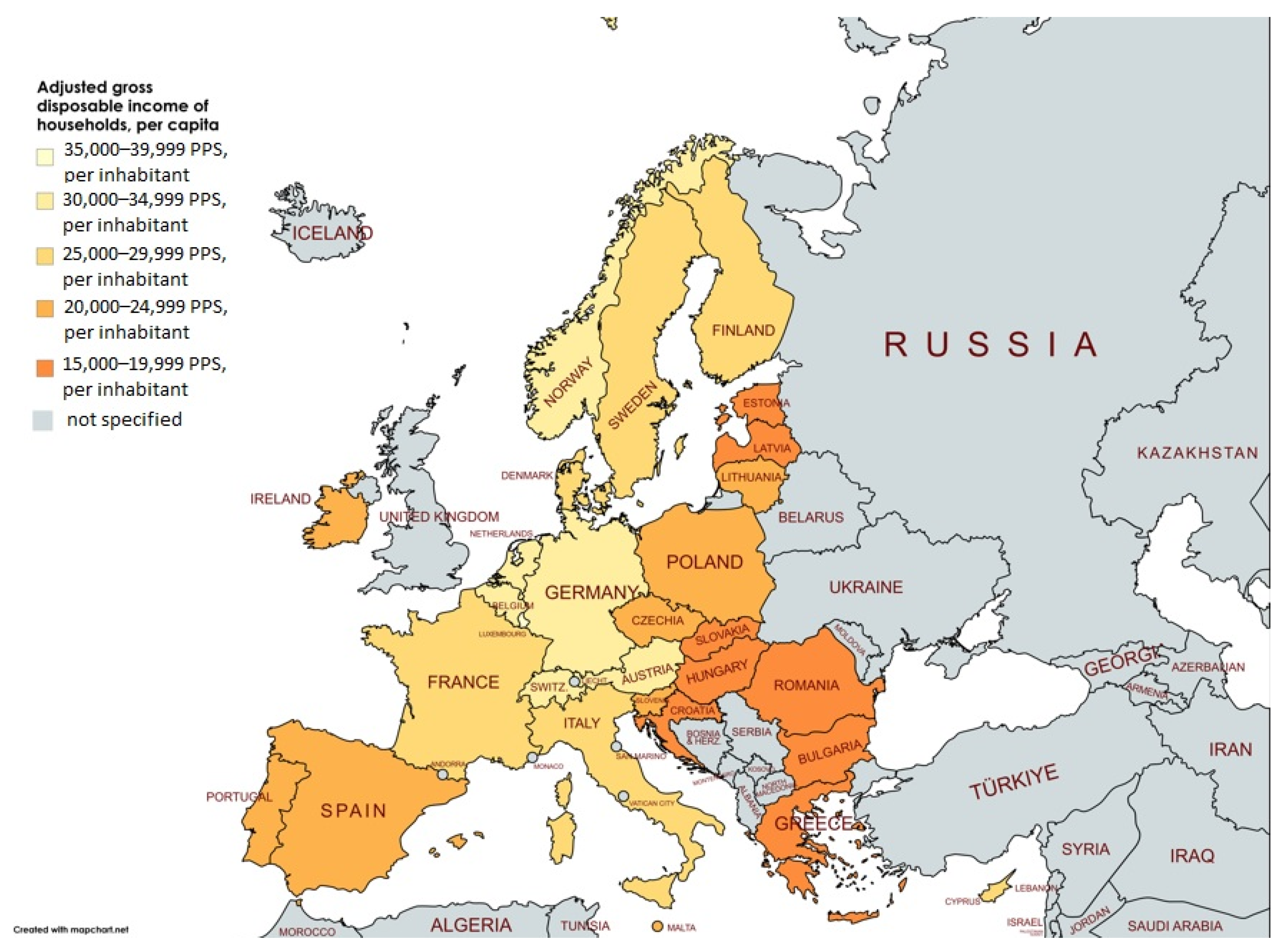
Figure 1. Adjusted gross disposable income of households, per capita, in European countries (2022). Created with Eurostat data, in MapChart v5.11.1.
Sustainability 17 09947 g001
Figure 2. Violin plots for each variable covering BG, CZ, EE, HU, LV, LT, PL, RO, SK, SI regions.
Sustainability 17 09947 g002
Figure 3. Correlation plot covering BG, CZ, EE, HU, LV, LT, PL, RO, SK, SI regions.
Sustainability 17 09947 g003
Figure 4. Disposable income of private households in NUTS2 regions in CEE countries (2022). Created with Eurostat data in MapChart.
Sustainability 17 09947 g004
Figure 5. Comparison of socioeconomic indicators (mean values) by region.
Sustainability 17 09947 g005
Table 1. Brief comparison among studies. CEE—Central and Eastern Europe; EU—European Union; GB—Great Britain.
Ref.ObjectiveTerritoryTime IntervalResults
Ref. [37]Factors that determine changes in income inequality10 CEE countries1989–2001Income inequality is mainly related to the privatization process, the social exclusion of minorities, and foreign capital investments.
Ref. [14]Relationship between industrial restructuring and economic growthCEE countries2004–2012Regional growth differences are due to productivity inequalities in higher-value sectors.
Ref. [30]Relationship between spatial and social disparities276 EU regions2000–2016Regional inequalities are related to the geography of production.
Ref. [43]Relationship between output expansion and unemployment13 Greek regions1971–1993A long-run relationship documented between unemployment and output growth. Okun’s law con-firmed for 6 out of the 13 regions examined.
Ref. [44]Influence of sociodemographic predictors and relative income147 EU regions1998–2012More levels of education are associated with lower heat-related mortality, while higher life expectancy and relative income have mixed relations.
Ref. [28]Evaluation of the dynamics of social and economic development41 GB regions2012–2020The leader in socioeconomic development among GB regions is London, which dominates economically over other regions.
Ref. [40]Outline regional disparities in developmentNUTS2 regions in Poland2010–2012; 2020–2022Authors highlighted clear spatial and structural disparities. Mazowieckie, which includes the capital city, importantly diverges in its level of social and economic development from the other regions.
Table 2. Variable specifications.
VariableAcronymMeasurement UnitSource
Disposable income of private households by NUTS2 regionINCMillion purchasing power standards (PPS, EU27 from 2020)Eurostat
Gross fixed capital formation by NUTS2 regionGCFCMillion euroEurostat
Unemployment rates by NUTS2 regionUNEMP% of population from 20 to 64 yearsEurostat
Population density by NUTS2 regionPOPPersons per square kilometerEurostat
Life expectancy at birth by NUTS2 regionLIFEEXPYearEurostat
Educational attainment level by NUTS2 regionEDUC% of population with tertiary educationEurostat
Youth employment rate by NUTS2 regionYEMP% of population from 25 to 29 yearsEurostat
Table 3. Descriptive statistics.
EDUCUNEMPYEMPLIFEEXPPOPGFCFINC
Mean26.096.1774.6376.57238.054840.7619,701.63
Median23.85.475.576.589.43946.3516,415
Maximum62.118.491.382.83448.131,298.5776,303.39
Minimum11.21.250.169.529.7408.023981.8
Std. Dev.9.883.367.052.06572.993723.5312,189.21
Skewness1.110.84−0.560.124.512.601.89
Kurtosis4.133.303.353.2522.8912.627.14
Table 4. Cross-sectional dependence test results (NUTS2 level covering BG, CZ, EE, HU, LV, LT, PL, RO, SK, SI).
TestsStatisticp-Value
Breusch–Pagan LM5240.380.000
Pesaran–scaled LM66.670.000
Pesaran CD9.420.000
Table 5. Panel unit root tests (NUTS2 level covering BG, CZ, EE, HU, LV, LT, PL, RO, SK, SI).
At Levels
INCGCFCUNEMPLIFEEXPPOP
Unit root (Common Unit Root Process)
LLC12.81
(0.99)
5.78
(0.99)
3.07
(0.998)
49.16
(0.999)
0.59
(0.723)
Unit root (Individual Unit Root Process)
IPS14.27
(0.99)
7.64
(0.99)
1.17
(0.879)
4.50
(0.999)
3.39
(0.999)
ADF-Fisher Chi-square3.19
(0.99)
57.10
(0.999)
87.30
(0.959)
21.68
(0.999)
115.11
(0.401)
At first difference
Unit root (Common Unit Root Process)
LLC−6.72
(0.000) *
−20.60
(0.000) *
−3.84
(0.000) *
−14.57
(0.000) *
−10.59
(0.000) *
Unit root (Individual Unit Root Process)
IPS−4.11
(0.000) *
−7.66
(0.000) **
−1.71
(0.043) **
−9.72
(0.023) **
−2.40
(0.008) *
ADF-Fisher Chi-square188.09
(0.000) *
278.25
(0.000) *
244.09
(0.000) *
323.968
(0.000) *
164.31
(0.009) *
*, ** significant at 1%, and 5% level.
Table 6. Results of Pedroni cointegration tests (NUTS2 level covering BG, CZ, EE, HU, LV, LT, PL, RO, SK, SI).
Pooled AR Coefficients Within-Dimension
Statistics (Prob.)Weighted Statistics (Prob.)
Panel v-stat.0.90 (0.183)−3.07 (0.99)
Panel ρ-stat. 4.58 (0.99)5.62 (0.99)
Panel PP-stat.−8.40 * (0.000)−11.52 * (0.000)
Panel ADF-stat. −6.89 * (0.000)−7.22 * (0.000)
Individual AR Coefficients Between-Dimension
Group ρ-stat.8.98 (0.99)
Group PP-stat.−17.94 * (0.000)
Group ADF-stat. −6.22 * (0.000)
* significant at 1% level.
Table 7. Results of Kao cointegration test (NUTS2 level covering BG, CZ, EE, HU, LV, LT, PL, RO, SK, SI).
t-StatisticProb
Variance ratio 0.001−3.340.000 *
* significant at 1% level.
Table 8. Panel ARDL (1,1,1,1,1) (NUTS2 level covering BG, CZ, EE, HU, LV, LT, PL, RO, SK, SI).
VariableCoefficientStd. Errort-StatisticProb. *
Long-Run Equation
GFCF1.310.0619.590.000 *
UNEMP−755.4115.01−50.300.000 *
LIFEEXP−1111.7354.90−20.370.000 *
POP1288.8629.8743.130.000 *
Short-Run Equation
COINTEQ01−0.120.06−2.070.039 **
D(GFCF)0.110.130.890.369
D(UNEMP)−41.1170.37−0.580.559
D(LIFEEXP)196.1472.772.690.007 *
D(POP)−265.39252.53−1.050.294
C−5690.74838.74−1.170.240
*, ** significant at 1%, and 5% level.
Table 9. Granger panel causality test (NUTS2 covering BG, CZ, EE, HU, LV, LT, PL, RO, SK, SI).
Null Hypothesis (H0)F-Statisticp-ValueConclusion
GCFC nGC INC6.120.002 *GCFC → INC
INC nGC CGFC5.830.003 *INC → GCFC
UNEMP nGC INC6.620.001 *UNEMP → INC
INC nGC UNEMP7.260.008 *INC → UNEMP
LIFEEXP nGC INC3.460.032 **LIFEEXP → INC
INC nGC LIFEEXP4.470.011 **INC → LIFEEXP
POP nGC INC2.060.128
INC nGC POP2.250.105
UNEMP nGC GCFC1.650.192
GCFC nGC UNEMP2.090.124
LIFEEXP nGC GFCF7.650.000 *LIFEEXP ⟶ GFCF
GFCF nGC LIFEEXP4.940.007 *GFCF → LIFEEXP
POP nGC GFCF7.560.000 *POP → GFCF
GFCF nGC POP4.940.007 *GFCF → POP
LIFEEXP nGC UNEMP5.500.004 *LIFEEXP → UNEMP
UNEMP nGC LIFEEXP11.162 × 10−5 *UNEMP → LIFEEXP
POP nGC UNEMP2.090.123
UNEMP nGC POP1.710.181
POP nGC LIFEEXP1.080.339
LIFEEXP nGC POP1.290.275
*, ** significant at 1%, and 5% level. “nGC” stands for” does not Granger cause”.
Disclaimer/Publisher’s Note: The statements, opinions and data contained in all publications are solely those of the individual author(s) and contributor(s) and not of MDPI and/or the editor(s). MDPI and/or the editor(s) disclaim responsibility for any injury to people or property resulting from any ideas, methods, instructions or products referred to in the content.