Article

Landscape Preferences of Recreational Walkways in Urban Green Spaces: Bada Shanren Meihu Scenic Area, China

1
College of Forestry, Jiangxi Agricultural University, Nanchang 330045, China
2
College of Life Sciences and Food Engineering, Huaiyin Institute of Technology, Huai’an 223003, China
3
Jiangxi Rural Cultural Development Research Center, Jiangxi Agricultural University, Nanchang 330045, China
*
Author to whom correspondence should be addressed.
Sustainability 2025, 17(22), 9931; https://doi.org/10.3390/su17229931
Submission received: 19 September 2025 / Revised: 11 October 2025 / Accepted: 19 October 2025 / Published: 7 November 2025

Abstract

Urban greenway trails serve as a vital link between urban populations and the natural environment, playing a key role in enhancing quality of life and promoting physical and mental well-being. We propose an interpretable machine learning framework applied to 424 geotagged footprint images from the Bada Shanren Meihu Scenic Area in China. Our main findings are as follows: (1) The key factors influencing trail landscape preferences include the Water Visibility Index (WVI), Building Landscape Index (BVI), Freedom Index, and Greenery Visibility Index (GVI). (2) For WVI, SHAP values significantly increase around the 0.05 threshold. BVI has a critical threshold of 0.17, with a strong influence below it and a reduced effect above it. The Freedom variable shows an inverse relationship, with minimal contribution below 0.21 and a sharp increase above this threshold. GVI maintains high SHAP values at lower levels (GVI ≤ 0.66), but its predictive utility decreases at higher values. (3) Landscape preferences are significantly positively correlated with naturalness, wildness, WVI, and openness, with water landscapes being the strongest driver. In contrast, artificial factors, V_Low, and H_Purple significantly suppress preferences. This suggests that human intervention and certain color tones may reduce the attractiveness of the landscape.

1. Introduction

Urban green spaces confer a multitude of advantages upon human well-being, encompassing both physical and mental health as well as social benefits [1,2]. The act of visiting green spaces presents an opportunity for individuals to directly experience the merits of the “natural” ecosystem, particularly for urban dwellers with restricted exposure to the natural environment [3]. This experience is, in essence, a multi-sensory process of landscape perception. As underscored in the European Landscape Convention, the essence of a landscape extends beyond its physical manifestation; it resides in the meaning construction bestowed by human subjects through visual engagement [4]. Nonetheless, the rapid pace of urbanization has exacerbated issues such as visual pollution, conflicts between artificial and natural elements, and the divergence between public preferences and landscape design [5]. Visual Landscape Assessment (VLA), an essential regulatory approach for enhancing the quality of the human settlement environment, has its core essence in the systematic analysis of the multi-dimensional interaction mechanism between landscapes and individuals [6,7]. Through the visual perception pathway, VLA undertakes the scientific identification and value evaluation of the external morphology and functional attributes of landscape spaces.
This research field investigates interactions between objective visual elements and subjective human perceptions. Objective elements comprise tangible natural and artificial components that shape human perception [8]. Measuring subjective perceptions in relation to these elements helps define and validate the role of visual features in environmental experience. Current studies typically examine either objective visual elements or subjective perceptions, but rarely both. Some research has employed regression analysis to investigate their correlations. However, this approach remains inadequate. It creates two practical challenges: (1) existing metrics often fail to detect visual quality deterioration, and (2) design decisions rely heavily on expert evaluation, potentially amplifying subjective bias [9]. Therefore, there is an urgent need for a framework that both quantifies the objective composition of landscapes and provides an interpretable connection to public preferences. This framework should address the questions, “Which landscape elements most drive preferences?” and “Can the method of surpassing correlation analysis better explain its relationship?”
A review of the theoretical spectrum reveals that VLA (Visual Landscape Assessment) has formed four complementary paradigms. The psychophysical paradigm treats landscape esthetics as a stimulus-response process, developing scales such as SBE and LCJ to rank landscape quality based on consistency judgments. The expert paradigm emphasizes evaluations based on formal esthetic principles by trained professionals, integrated with GIS [10], imaging, and visual resource management technologies to support planning decisions. The cognitive paradigm focuses on the coupling between landscapes and cognitive/emotional responses, using indicators such as PRS [11], POMS [12], and EEG/ECG to enhance validity. The experiential paradigm highlights how individual traits and cultural contexts shape esthetic judgments [13,14].
While many traditional methods are still in use, advancements in tools and technologies—such as public participation platforms (PPGIS) [15], street-view imaging [16], visitor tracking [17], and eye-tracking [18,19,20]—have significantly improved analytical precision and result accuracy. Notably, in recent years, image semantic segmentation technology has been widely applied in landscape research, particularly in areas such as land cover detection, landscape ecology, and street scene analysis.
Building on these advancements, this study proposes an innovative framework that quantifies the objective composition of landscapes and establishes an interpretable connection to subjective preferences. The RF-SHAP framework overcomes the limitations of regression analysis by utilizing random forest (RF) to capture nonlinear relationships and interactions among landscape elements. Additionally, the SHAP method enhances interpretability by providing insights into the individual contributions of each element, reducing reliance on expert judgment and offering a more objective and scalable approach for landscape analysis. First, semantic segmentation is used to perform pixel-level quantification of landscape elements in images [6,21,22]. Then, a random forest model is employed to predict subjective preference scores, while SHAP (Shapley Additive Explanations) is introduced to attribute model outputs and identify the key environmental features driving preferences, along with their nonlinear and interactive effects.
Compared to traditional methods, this framework offers three key contributions. First, it bridges the gap between objective landscape composition and subjective preferences, providing a consistent quantitative link. Second, it goes beyond linear correlation to reveal complex mechanisms of action and offers interpretable evidence at the element level. Third, it provides actionable strategies for design and management, supporting early identification of visual quality risks and precise optimization of element configurations, ultimately enhancing the experiential quality and sustainability of pathway landscapes.

2. Materials and Methods

2.1. Research Scope

The Bada Shanren Meihu Scenic Area, situated in Qingyunpu District, Nanchang City, Jiangxi Province, constitutes a multidimensional cultural landscape (Figure 1). This study selects it as an exemplary case based on three defining characteristics: In terms of geographic spatial background, functioning as Nanchang’s southern gateway cultural nexus, it constitutes a critical node in the Ganpo Cultural-Ecological Corridor. This site simultaneously preserves urban cultural continuity and establishes ecological networks. In terms of cultural heritage value, housing China’s most intact surviving Ming loyalist artistic heritage sites, it serves as the memorial complex for Zhu Da (Bada Shanren)—a pinnacle figure in Chinese freehand painting. The well-preserved Ming-Qing architecture cluster embodies the materialized expression of Eastern esthetic philosophy. In terms of ecological recreation, the scenic area is linked by the Meihu Lake system, with a water surface area of approximately 45.62 hectares. Through dredging and water system connection projects, it has formed a meandering river and lake landscape, attracting numerous tourists every year. Through analyzing the visual preference mechanisms of its trail landscapes, this research proposes universal optimization strategies for sustainable management of analogous cultural landscapes.

2.2. Experimental Procedure

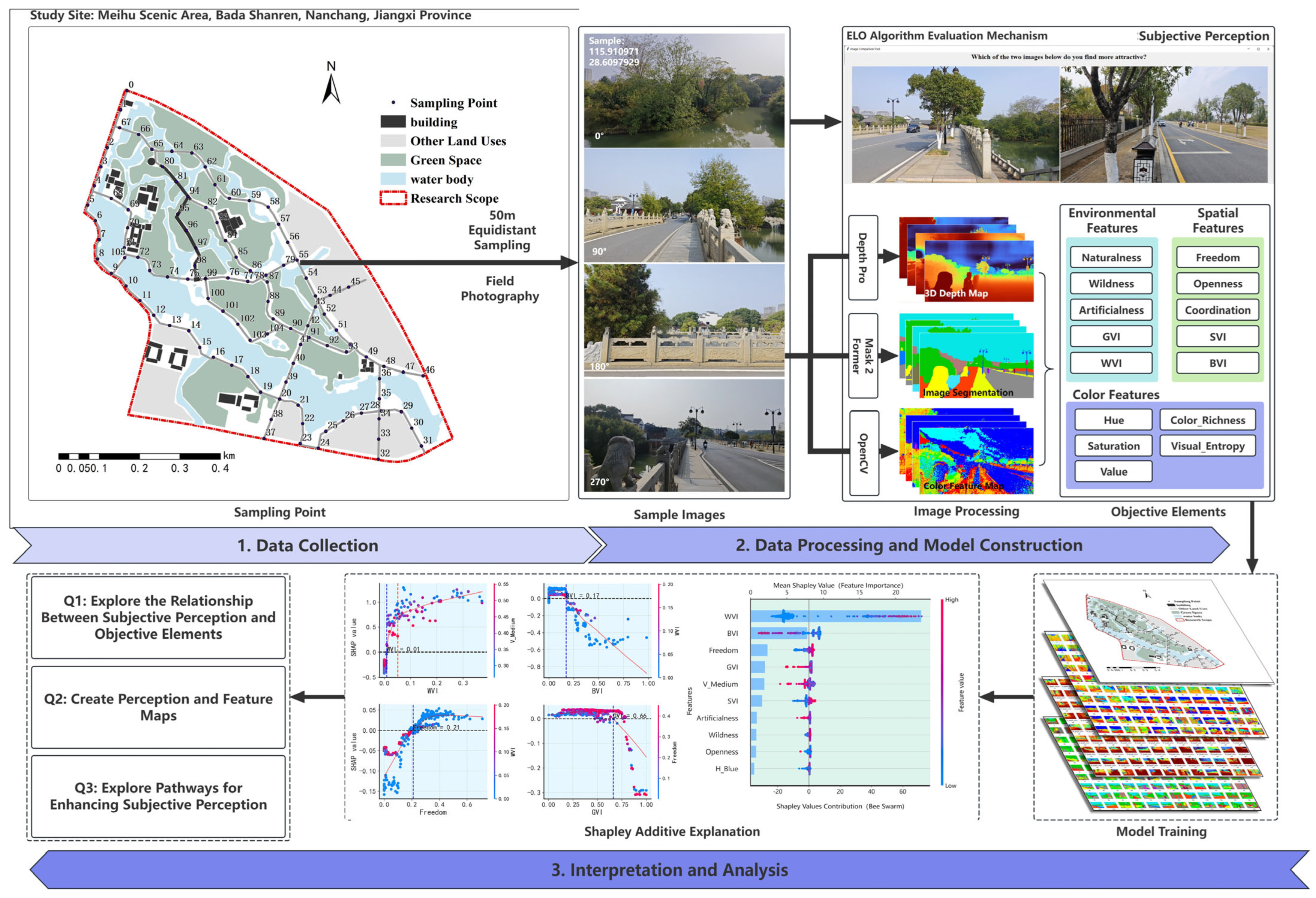
To empirically evaluate the visual quality of walking trails in the Bada Shanren Scenic Area, this study first plotted the trails using the official site maps in ArcGIS (version 10.8). Employing the ArcPy module, sampling points were generated every fifty meters along each trail, resulting in one hundred six sample points. The determination of this 50 m interval was based on a comprehensive evaluation of regional characteristics, prior research experience, and data collection/analysis feasibility. The trail landscape in Badashanren Scenic Area exhibits distinct spatial coherence and a relatively stable configuration. This selected spacing ensures adequate coverage of typical variations among diverse landscape elements within the study area. On 8 December 2024 (weather: clear), images were captured at each sample point from four azimuth angles (0°, 90°, 180°, 270°) at a standardized height of 1.6 m, producing a total of four hundred twenty-four images for visual quality assessment. Depth Pro, Mask2Former, and the OpenCV library were then utilized to derive depth maps, perform image segmentation, and extract color features. The resulting objective features were integrated with subjective evaluations and modeled using RF. A SHAP (SHapley Additive exPlanations) analysis was then conducted to interpret the model’s outputs. The complete workflow is depicted in Figure 2.

2.3. Related Methods

2.3.1. ELO Evaluation Algorithm

Visual subjective evaluation primarily investigates the relationship between images and the reactions they elicit, as well as the differences in responses among various groups [23]. Traditional methods, such as Semantic Differential Evaluation (SBE) and Likert Scale Judgment (LCJ) [24,25,26,27], often face reliability concerns due to subjective score variations among different evaluators when rating identical images. To address this issue, this study employs the ELO Rating System, which facilitates subjective image evaluations through pairwise comparisons. Participants are tasked with selecting between randomly presented image pairs, a method that has been scientifically validated by researchers such as Goodspeed [28]. Compared to the SBE and LCJ methods, the ELO system offers two major advantages: it supports direct comparisons, as in the LCJ method, and mitigates evaluator bias, similar to the SBE method, thereby enhancing result consistency and reliability. In this research, the ELO rating system was realized via a Python 3.11 program, aiming to quantify the disparities in tourists’ preferences for the images of the scenic area. At the initial stage, an identical baseline score (with an initial ELO value of 1000) was assigned to all images. During the experimental process, the system randomly selected two images for juxtaposition. Participants were obligated to make a choice grounded in their subjective judgment regarding “which image is more appealing”. This criterion was designed to capture tourists’ immediate impressions, interests, and emotional stances towards the scenic area, rather than a mere assessment of “beauty” from an esthetic perspective. As an important part of visual perception, landscape attractiveness reflects individuals’ active recognition and selection of landscape spaces, and also determines the objective scope and degree to which landscape elements exert an attraction on individuals.
Prior to the commencement of the experiment, participants were required to peruse the guidelines and complete the training session, so as to clarify the operational definition of “attractiveness”. In this study, “attractiveness” is predominantly defined as the intensity of positive emotions (such as a sense of yearning and delight) elicited by the image. To enhance the data quality and minimize redundancy, an adaptive sampling strategy was incorporated into the program. This strategy gave precedence to image pairs that had not been compared for an extended period. Such an approach optimized the data collection process, diminished redundant comparisons, and augmented the efficiency and flexibility of the experiment.
To ensure the scientific rigor and accuracy of the data, participants must meet the following screening criteria: all participants must have normal color vision, with no color blindness or color weakness; they must possess normal cognitive abilities, free from cognitive impairments or neurological disorders, and be capable of understanding and performing the experimental tasks. Additionally, participants with backgrounds in landscape design, urban planning, or related fields are excluded to prevent professional knowledge from influencing preference judgments. The participant pool comprised 62 subjects, ensuring the diversity and representativeness of the evaluation outcomes. Their demographic characteristics are presented in the subsequent Table 1.
In the ELO Rating System, the comparison results dynamically update the image scores. Specifically, the system calculates a “win-loss score” based on the current scores of the images. When an image wins, its score increases, and when it loses, its score decreases. Over multiple pairwise comparisons, the ranking difference (Rank_diff) between the images stabilizes. Although all images start with the same initial score, this initial score only affects the starting point and does not influence the final relative ranking or score differences.

2.3.2. Depth Pro Model

Depth Pro was selected for its zero-shot monocular depth estimation from single RGB images, providing efficient processing without the need for specialized hardware, ideal for analyzing field-captured trail photos in this study. Depth Pro, developed by Apple, is a zero-shot monocular depth estimation model capable of generating high-resolution 3D depth maps from a single 2D image in approximately 0.3 s. Its source code is available at https://github.com/apple/ml-depth-pro (accessed on 20 December 2024). The model’s innovations include a multi-scale Vision Transformer (ViT) architecture, zero-shot learning capabilities, and enhanced boundary and detail extraction [29]. By integrating advanced deep learning algorithms with convolutional neural networks (CNNs) and efficient data processing frameworks, Depth Pro achieves near-instantaneous image conversion. Compared to hardware-based systems like LiDAR, which provide millimeter-precision but require specialized equipment and extensive fieldwork, Depth Pro offers sufficient accuracy for visual landscape analysis with advantages in speed, cost, and flexibility from single images. Unlike immediate depth capture from Time-of-Flight (ToF) cameras, Depth Pro’s 0.3 s time reflects software processing on a standard GPU for 2.25-megapixel maps, making it suitable for post-field analysis of monocular photos. This monocular RGB-based framework enables cost-effective depth estimation without requiring specialized sensors. Ongoing enhancements to its zero-shot generalization capabilities suggest its potential as a viable alternative to conventional spatial sensing approaches. Specific applications in landscape terrain modeling, augmented reality (AR)-enhanced site analysis, autonomous robotic navigation, and medical imaging diagnostics highlight its cross-domain adaptability.
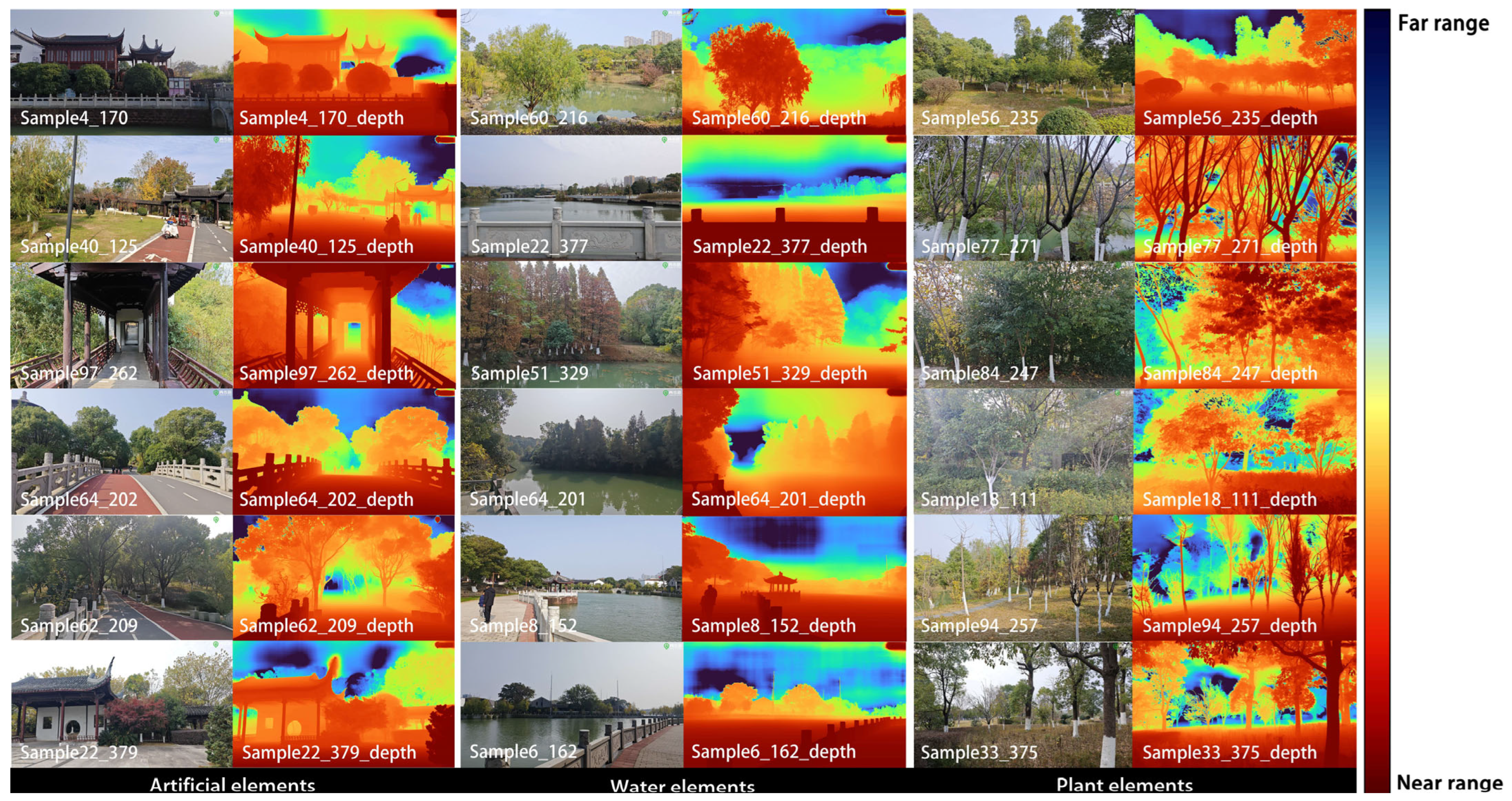
In Figure 3, we demonstrate the application of this algorithm to generate a depth map from two-dimensional images of the study site. The method effectively captures depth information for built, aquatic, and vegetative elements. The resulting depth map is rendered using a color gradient ranging from dark blue to dark red. Pixels closer to dark blue are located farther from the camera, while those closer to dark red appear nearer. Ultimately, the mean depth of all elements in the image is calculated to represent environmental openness.

2.3.3. Mask2Former Model

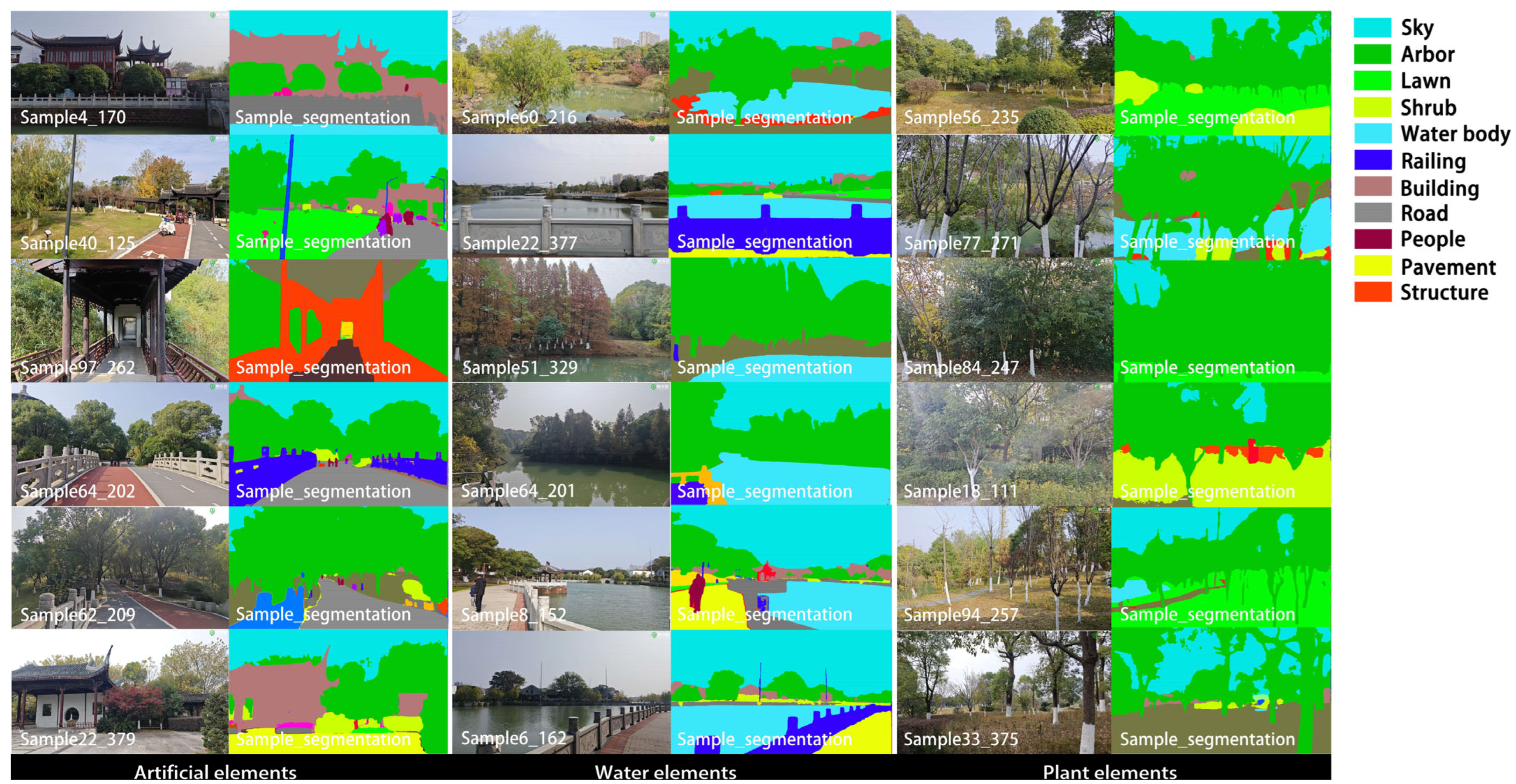
Mask2Former was chosen for its high accuracy in semantic and instance segmentation of complex natural scenes, leveraging Transformer architectures trained on the ADE20K dataset, which supports detailed landscape element analysis. Mask2Former is a deep learning model specifically designed for image segmentation tasks, notably instance and semantic segmentation [30]. It incorporates Transformer-based architectures into traditional segmentation workflows, emphasizing more efficient mask generation. The training dataset utilizes ADE20K, a benchmark dataset released by MIT in 2017. This dataset supports multiple computer vision tasks including scene perception, image parsing, semantic segmentation, multi-object recognition, and semantic understanding. Its hierarchical annotation structure enables both pixel-level accuracy assessment and holistic scene comprehension. These characteristics make it particularly valuable for landscape pattern analysis and vegetation segmentation applications. Consequently, Mask2Former achieves higher accuracy, particularly in complex settings and multi-object instance segmentation scenarios. The segmentation effect of the model is shown in Figure 4.

2.3.4. Quantification of Color Elements

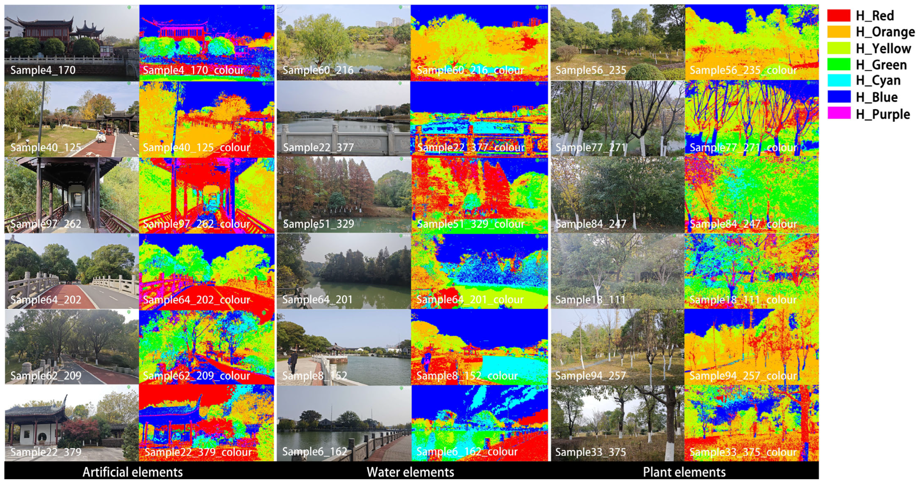
This study adopts an HSV-based image feature extraction method for automated batch processing and metric computation. First, images are converted from the BGR to the HSV color space using OpenCV, which better aligns with human visual perception. Next, we calculate and normalize pixel distributions for red, orange, yellow, green, cyan, blue, and purple according to predefined hue, saturation, and value ranges, thereby quantifying the proportion of each color (Figure 5). We also compute the mean and standard deviation of pixel values to derive color richness (Color_Richness), indicating the overall diversity of colors within an image. Finally, we employ grayscale histogram entropy to measure visual entropy (Visual_Entropy) [31]. Initially introduced to depict disorder in thermodynamics, entropy has been increasingly used in graphics to describe the subjective perception of detail and structural complexity.

2.3.5. Machine Learning Modeling Methods

Nonlinear machine learning fitting establishes relationships between feature variables and known sample categories through model construction [32]. This approach autonomously learns complex patterns and identifies latent data characteristics [33]. By training and optimizing models, it facilitates the discovery of hidden data regularities and trends, thereby providing scientific foundations for decision-making. To identify the most suitable algorithm, six prevalent machine learning classifiers were evaluated: Decision Trees (DT), Random Forest (RF), Support Vector Machine (SVM), Logistic Regression (LR), K-Nearest Neighbors (KNN), and eXtreme Gradient Boosting (XGBoost) [34]. The study established predefined search spaces encompassing core hyperparameters. A systematic grid search coupled with 5-fold cross-validation was implemented to identify optimal parameter configurations for each algorithm, ultimately constructing performance-optimized regression models.

2.3.6. SHAP Model

SHAP (SHapley Additive exPlanations), introduced by Lundberg and Lee [35], is a widely utilized framework for model interpretability in machine learning. Rooted in cooperative game theory’s Shapley values, SHAP quantifies each feature’s contribution and direction (positive or negative) to a model’s predictions. While complex models (e.g., deep neural networks, XGBoost) achieve high predictive accuracy, their opaque “black box” nature impedes transparent interpretation. By assessing feature importance, SHAP elucidates these predictive mechanisms, making it suitable for both regression and classification models [36]. It enables interpretation from both global and local perspectives, thereby enhancing the trustworthiness and applicability of complex machine learning models. SHAP thus serves as a pivotal methodology for mitigating the interpretability challenges of advanced predictive modeling. The computational approach for Shapley values is as follows:
φ i ( f ) = S N \ i | S | ! ( | N | - | S | - 1 ) ! | N | ! f ( S i ) f ( S ) ,
where N represents the complete set of features; S represents a subset of features;
f ( S ) is the model’s prediction result given the feature subset S ;
f ( S { i } ) is the model’s prediction result given the feature subset S with the addition of feature i .

2.4. Selection of Objective Indicators

Previous studies have rigorously examined the concept of integrating subjective perception with visual landscapes by considering how individuals visually and psychologically engage with their surroundings [37]. Through this perspective, researchers have identified a range of factors that shape environmental preferences and have translated these factors into measurable and comparable indicators [38]. Drawing on theoretical frameworks from environmental psychology, visual perception, and architectural esthetics, this study classifies the indicators into three principal categories: “environmental characteristics”, “spatial characteristics” and “color characteristics”.
Within the spatial dimension, emphasis is placed on freedom [39,40], coordination, and the building view index [41]. In the environmental dimension, primary attention is given to the green view index [42], naturalness [43], water view index [44], and wildness [45,46]. Meanwhile, the color dimension encompasses variables such as hue [47], saturation, value, visual entropy, and color richness [48].
Although environmental and spatial characteristics both fall under the broader umbrella of “environment and design,” they diverge in emphasis. Environmental characteristics highlight “what is present in the landscape,” referring to visible elements and their inherent attributes, which directly influence individuals’ physiological and psychological responses [49]. By contrast, spatial characteristics address “how these landscape elements are arranged and organized to shape spatial experiences”, underscoring how people perceive the overall spatial form and relationships within an environment.
Building on these objective indicators and site-specific conditions, this study investigates the Bada Shanren area, ultimately deriving 25 indicators that span the three primary dimensions, as presented in Table 2.

3. Results

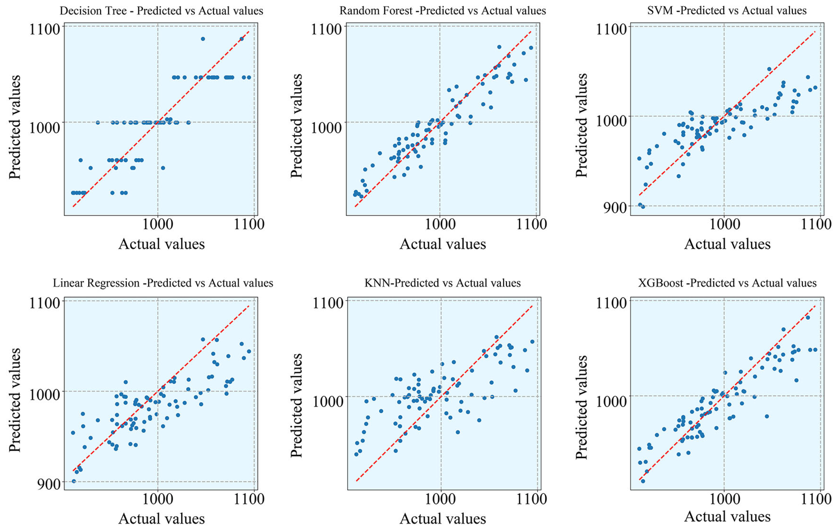
In this research, the model performance was evaluated comprehensively using the Mean Absolute Error (MAE), Mean Squared Error (MSE), Root Mean Squared Error (RMSE), and the coefficient of determination (R2). The findings revealed that the Random Forest algorithm (MAE = 13.62, MSE = 276.48, RMSE = 16.63, R2 = 0.875) outperformed the other five types of models (Table 3). As shown in Figure 6, the scatter plots of predicted versus true values for each model further corroborate this observation. The red dashed line represents the identity line (y = x); tighter clustering around this line indicates greater accuracy and smaller errors. With an R2 value of 0.875, the model was able to account for 87.5% of the variation in the target variable, significantly surpassing other models (e.g., SVM with an R2 of 0.618 and KNN with an R2 of 0.501). This performance superiority stemmed from the Random Forest’s parameter settings of max_depth = 6 and n_estimators = 100. These settings effectively captured the nonlinear interactions among multi-dimensional features while mitigating the risk of overfitting. Although XGBoost (R2 = 0.811) ranked second in performance, its explanatory power far exceeded that of traditional linear models (such as linear regression with an R2 of 0.582), further validating the suitability of ensemble learning methods for modeling complex landscape perceptions. Ultimately, considering the balance among error minimization, maximizing explanatory power, and ensuring robustness, this study chose the Random Forest as the core algorithm. Its high accuracy and stability furnished a solid foundation for the subsequent SHAP-driven attribution analysis.

3.1. Feature Contributions

Decision tree-based models, like random forests, are capable of automatically assigning feature importance. Nevertheless, their assignment mechanisms exert an influence on the analysis outcomes. It is crucial to note that there exists a fundamental distinction between feature importance and feature contribution. The former reveals which features have the most significant impact on the model’s prediction accuracy, whereas the latter offers an intuitive explanation of the formation mechanism behind numerical prediction results.
In this research, two analytical approaches are employed to assess the significance of each feature and its contribution to model prediction: the model-based feature importance analysis method and the feature importance analysis method grounded in the SHAP summary graph. Initially, the importance of each feature within the model is analyzed. The importance ranking graph depicted in Figure 7a primarily reflects the predictive ability of features during the regression analysis procedure. The cumulative sum of the importance weights of all features in the model amounts to 1. Among these, the top few variables with the highest importance scores are, in sequence, WVI, BVI, GVI, V Medium, and Freedom. However, it should be emphasized that this analysis result fails to illustrate the contribution level of each feature to specific numerical prediction outcomes. To address this, we further introduce the SHAP summary analysis for a more in-depth examination.
By means of the SHAP summary graph (Figure 7b), quantitative values that reflect the contribution of variables (i.e., aggregated Shapley values) can be derived. The x-axis of this graph showcases the contribution of each feature to the regression prediction result, based on the average sum of the absolute values of the SHAP values. The analysis indicates that the top few variables with the highest contribution to the model prediction are, in order: WVI [50], BVI, Freedom, GVI, and V_Medium, among others.

3.2. Feature Dependency Analysis

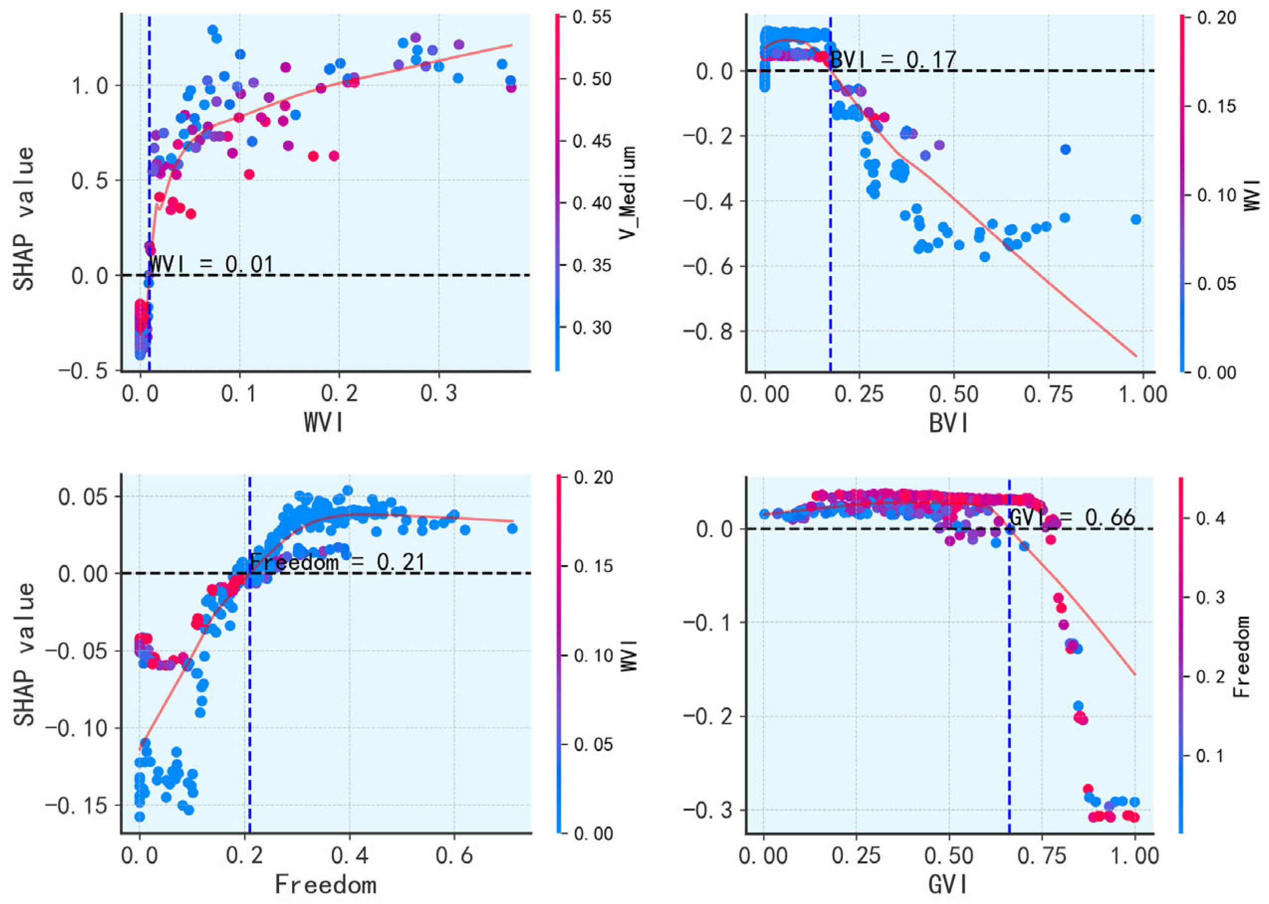
The SHAP dependence plots were analyzed to examine how input variable interactions contribute to the Random Forest (RF) model predictions. As depicted in Figure 8, the most striking trends in the SHAP dependence analysis results are related to the graphs of WVI, BVI, Freedom, and GVI. These graphs rank highly in terms of contribution based on the SHAP summary graph (see Figure 7b). The scatter plot of red and blue points illustrates the variations in the SHAP values of WVI. In the graph, around 0.05 (the vertical red line), the variation trends of the SHAP values of WVI are evident. When the water view rate of the site is low (WVI < 0.05), increasing the proportion of water features in the site (e.g., installing some water feature facilities) can significantly enhance the landscape preference [51]. Correspondingly, when the site already has a certain water view rate, increasing the proportion of water features has a negligible positive contribution to the outcome, and WVI peaks at approximately 0.1. Regarding BVI, when the building view index is below 0.17, the SHAP value of BVI is high, contributing substantially to the estimation of landscape preference. Conversely, when BVI exceeds 0.17, the SHAP value of BVI is low. For Freedom, when its value is less than 0.21, the SHAP value of Freedom is low. Conversely, when Freedom is greater than 0.21, it has a high SHAP value and makes a significant contribution to the estimation of landscape preference, reaching a peak around 0.3. Additionally, for GVI, the green view rate has always been a crucial element in previous studies. Nevertheless, in this study, it is discovered that when GVI is 0.66 or lower, high SHAP values are relatively evenly distributed. When GVI is greater than 0.66, the higher the GVI value, the lower the contribution to the landscape preference.

3.3. Spatial Distribution of Features

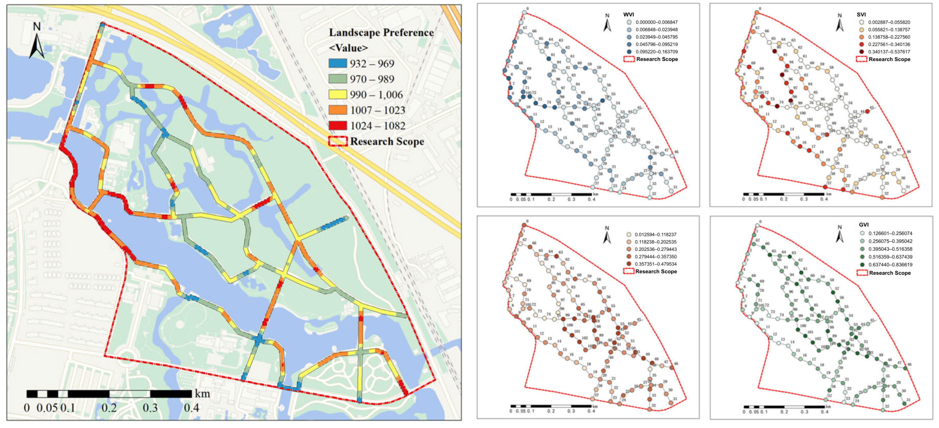
We calculated the average landscape preference for four images at each sampling point, and then visualized the landscape preferences along the trails of the scenic area using the Inverse Distance Weighting (IDW) method in ArcGIS. As shown in Figure 9. In the central portion of the Bada Shanren Scenic Area (points 80–93 and 94–104), landscape preference is relatively low, likely due to reduced water visibility, naturalness, and emptiness ratio. In contrast, the northern (46–67) and western (0–31 and 68–79) segments generally display higher levels of landscape preference. Nonetheless, several individual points (16, 20, 23, and 24) warrant targeted improvements. Based on the objective metrics mapped in this study, these locations are primarily characterized by low water visibility, sky visibility, and naturalness, coupled with high building sight index and artificiality. Therefore, targeted improvements should focus on these specific aspects to enhance the landscape quality.
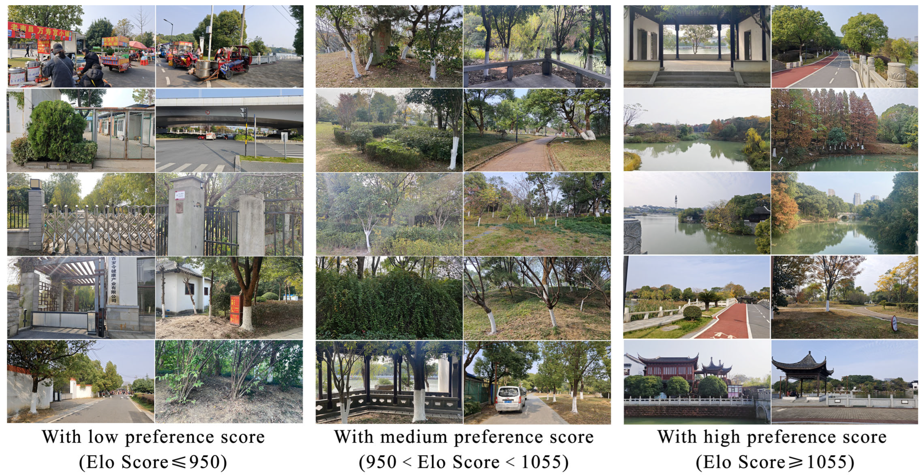
We differentiated the subjective preference Elo score, and Figure 10 shows representative images of high, medium, and low landscape preferences, arranged from low (left) to high (right) in order of preference level. The results align with intuitive expectations: images featuring greenery and water bodies received higher preference scores, while those containing artificial structures or exposed soil were consistently rated lower.
We analyzed the relationship between landscape preference scores and objective metrics using Spearman’s correlation analysis. As shown in Table 4, landscape preferences demonstrated significant correlations with multiple environmental indicators:
  • Positive correlations: Naturalness ( ρ = 0.156, p = 0.001), Wildness ( ρ = 0.117, p = 0.015), WVI ( ρ = 0.527, p < 0.001), and Openness ( ρ = 0.261, p < 0.001). Water features showed the strongest positive effect.
  • Negative correlations: Artificialness ( ρ = −0.23, p < 0.001), V_Low ( ρ = −0.105, p = 0.03), and H_Purple ( ρ = −0.129, p = 0.008), suggesting artificial elements and specific color tones reduce appeal.
Additional findings:
  • High brightness ( ρ = 0.245, p < 0.001) and blue tones ( ρ = 0.251, p < 0.001) enhanced preferences by increasing visual vibrancy and serenity, respectively.
  • Non-significant indicators (p > 0.05): Freedom and Coordination require further investigation.
Figure 11 quantifies the driving mechanisms of different features on landscape preference through SHAP contribution values. In the high-preference category, WVI and Freedom exhibit the most prominent contributions, with SHAP values of 0.065 and 0.064, respectively. This indicates that the visual accessibility of water landscapes and exploratory activities in open spaces are key factors enhancing visitor preference. In the medium-preference category, Freedom (0.048) and WVI (0.047) show similar contribution values. Meanwhile, Openness (Spatial Visual Diversity, 0.038) emerges as a significant factor, reflecting that moderately preferred landscapes require a balance between spatial openness and visual diversity. For the low-preference category, Artificialness acts as the primary negative driving factor, with a SHAP value of 0.106. Its contribution magnitude surpasses all other features, confirming the detrimental effect of artificial environments on scenic esthetic appeal.

3.4. Single-Sample Local Interpretation

To gain deeper insights into the results generated by individual samples within the SHAP model, we employed SHAP waterfall plots. By displaying each feature’s contribution to the predicted outcome, these plots offer an intuitive means of interpreting the decision-making process of complex models. A key advantage of such visualizations is that they not only illustrate the magnitude of each feature’s contribution to the model’s prediction but also reveal the direction of that influence, whether positive or negative. Although SHAP waterfall plots can be computationally expensive and may pose scalability challenges, they remain widely used in the academic community due to their value in model interpretation and feature contribution analysis.
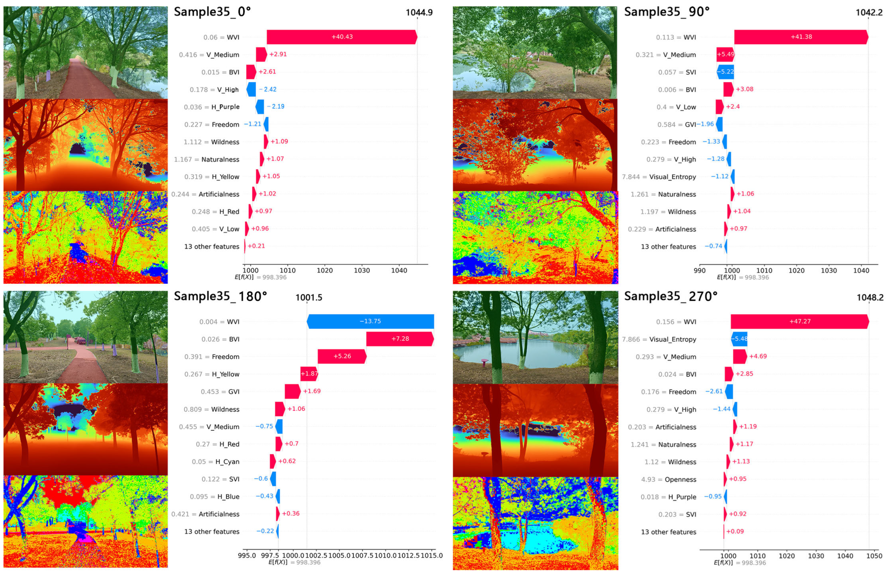
From the generalized results of landscape preference evaluations in the Bada Shanren Scenic Area, we randomly selected Sample No. 35, which includes four orientations (0°, 90°, 180°, and 270°; see Figure 12). The local interpretation results were visualized using the SHAP algorithm, where the vertical axis represents the variables and their respective feature values, and the horizontal axis indicates the magnitude and direction of their influence on the model. Blue denotes a suppressive effect, red denotes a promotive effect, and f(x) denotes the cumulative contribution of all factors, corresponding to the processed predicted value of the model.
This study identifies core predictive variables for the model, including WVI, BVI, Freedom, and V_Medium. In samples 35_0°, 35_90°, and 35_270°, increased WVI consistently enhanced landscape preference, aligning with Fry’s [52] prior findings. Conversely, sample 35_90° exhibited a low WVI value (0.004), yielding a moderate negative contribution. BVI and Artificialness demonstrated positive effects across all four perspectives, suggesting that trailside artificial amenities enhance attractiveness when visually balanced. The Freedom metric, measuring activity space autonomy, showed sample-specific effects: negative associations in 35_0°, 35_90°, and 35_270° stemmed from constrained spatial layouts, whereas sample 35_180°—featuring expansive lawns and meandering paths—showed positive correlations. All landscapes exhibited wilding traits, with Wildness scores contributing positively at varying intensities. SHAP single-sample waterfall plots quantify variable impacts in individual images, offering visual tools to identify detracting factors and inform targeted design improvements, thereby enhancing esthetic and experiential outcomes.

4. Discussion

We combine pixel-level semantic segmentation and Depth Pro depth estimates with a Random Forest regression model. The ensemble yields robust prediction and clear interpretability for trail landscape preferences. Across competing algorithms, RF achieved the strongest overall performance, consistent with the working hypothesis that nonlinear, interaction-aware models better accommodate the complexity of visual environments. Global and local SHAP analyses converge on several drivers: higher water visibility (WVI) and spatial freedom (Freedom) consistently elevate preferences; building visibility (BVI) and overall artificialness depress them once they exceed modest levels; and green view (GVI) exhibits diminishing returns rather than unbounded gains. These patterns reinforce a threshold-and-interaction view of landscape perception rather than simple linear dose–response assumptions.
Our findings align with long-standing evidence that blue–green cues and legible open vistas foster restorative and esthetic responses. The prominence of WVI is consistent with literature on biophilic and restorative affordances of water and sky, but the results refine those traditions by emphasizing visibility (i.e., unobstructed lines of sight) over mere presence. Similarly, the biophilic design patterns outlined by Browning et al. in “14 Patterns of Biophilic Design” highlight visual connections to nature, such as water and open vistas, as key to well-being—corroborating our WVI prominence while refining it to prioritize unobstructed sightlines over static presence [53]. The Freedom effect extends work on spatial legibility and choice by showing that opportunities to move, pause, and explore function as positive affordances that amplify preference when paired with adequate enclosure and sightlines. These observations on WVI and Freedom resonate with classical theories such as Prospect-Refuge Theory, which posits that humans prefer landscapes offering opportunities for prospect (open views) and refuge (enclosure), thereby enhancing perceived safety and esthetic pleasure [54].
At the same time, the observed saturation of GVI challenges a common simplification that “more greenery is always better”. When greenery occludes sky/water or increases visual uniformity, preferences plateau or decline—consistent with theories that emphasize balance among coherence, complexity, and prospect. Likewise, the dual role of built elements corroborates prior reports: well-placed, visually quiet structures can support wayfinding and activity, but excessive massing or high-contrast façades raise visual entropy and crowd out blue–green cues. Peters and D’Penna in “Biophilic Design for Restorative University Learning Environments” link prospect (open sightlines) and refuge (enclosure) to preference amplification in built settings, paralleling our observations of Freedom’s role when paired with blue-green cues and providing evidence-based design implications for trail landscapes [55].
In addition, this work highlights the difference between feature importance (which improves global fit) and feature contribution (which explains individual predictions). Model-embedded importances alone can mislead when features interact; SHAP complements them by revealing direction, magnitude, and context of effects. Nonetheless, SHAP assumes a background distribution and may over- or under-attribute in the presence of correlated features. Best practice therefore combines multiple diagnostics and checks stability across resamples and background sets.

4.1. Impact and Contributions on Planning and Design

The explainable learning framework developed here offers an operational bridge from objective scene composition to subjective preference. Rather than prescribing universal recipes, the results indicate threshold-aware and interaction-sensitive guidelines. In our study context, water visibility (WVI) exhibited strong positive effects that attenuate beyond a modest range, green view (GVI) displayed diminishing returns at high levels, building visibility (BVI) became detrimental past a low-to-moderate threshold, and spatial freedom (Freedom) was consistently beneficial once a minimum affordance level was achieved. These inflection zones should be interpreted as calibration priors for local application, to be verified with site-specific sampling and iteration. Because the recommended thresholds are conditional and context-dependent, planning should institutionalize adaptive cycles. Include fixed-vantage seasonal imagery in evaluations to refresh the baseline of subjective preferences.
Consistent with restorative environment theory, natural vistas—especially water and sky—are primary drivers of landscape preference. The model shows that raising the Water Visibility Index (WVI) from very low baselines yields large gains. Beyond a mid-range, additional increases offer limited benefits. Planning should therefore prioritize visibility to water: select tall-crowned vegetation, control railing heights along shorelines, and introduce small, visibly accessible waterscapes before expanding total water surface area. Where visibility is already sufficient, investment should shift from enlarging area to improving waterfront edge quality. Over-programming or excessive formalization may erode the very qualities that support preference.
GVI remains a robust positive cue, but the observed saturation cautions against equating higher GVI with monotonically higher quality. Dense, uniform canopies or continuous shrub screens can occlude sky and water and compress sightlines, thereby reducing perceived depth and exploratory potential. Planting design should pursue structural diversity (layered canopies, mixed leaf forms, seasonal contrast) while safeguarding visual permeability through lifted crowns, intermittent shrub masses, and “windowed” openings aligned with key vistas. Where heat stress or glare is a concern, shading objectives can be met with canopy architecture and deciduous species selection rather than blanket densification that undermines openness.

4.2. Limitations

Several limitations constrain the study’s generalizability. We analyzed a single scenic trail within one urban green space. External validity across cities, cultures, and landscape types remains to be established. Image acquisition was cross-sectional, with limited control over season, time of day, occupancy, and weather. These factors can shift user preferences. Nevertheless, they do not materially affect the interpretation of the findings or the decision logic of the proposed model.

5. Conclusions

As urbanization accelerates, enhancing the quality of urban green spaces to meet public esthetic expectations and foster harmonious human–nature interactions has emerged as a critical research focus [56]. Understanding the key determinants of landscape preference along walking trails facilitates more user-oriented and context-specific design interventions, thereby supporting the sustainable development of scenic areas. Our study of the Badashanren Scenic Trail shows that water visibility (WVI), building visibility (BVI), spatial freedom, and the green view index (GVI) interact in nonlinear ways to shape landscape preferences. These findings address gaps in interpretability and support broader sustainability goals by guiding user-centered interventions that improve restorative benefits and biodiversity in urban environments.
This research leverages the RF-SHAP framework to develop an interpretable model for visual landscape preference assessment, overcoming limitations in traditional methods’ data handling and explanatory power. Through global and local analyses of factor contributions, spatial patterns, and correlations, the integrated findings highlight a multifaceted view of preference formation, where environmental cues like naturalness and openness amplify appeal while artificial elements may detract.
Key synthesized outcomes include the following:
(1)
Superior Performance of Random Forest Model: The Random Forest (RF) algorithm outperformed the other five models (MAE = 13.62, MSE = 276.48, RMSE = 16.63, R2 = 0.875). It explained 87.5% of the target variable’s variance, demonstrating high accuracy and reliability in trail landscape preference assessment. By integrating the SHAP-RF method, this study quantified the contribution and importance of influencing factors at both global and local levels. The approach provides a scientific tool for landscape preference modeling and enhances the interpretability of machine learning models in theory and practice.
(2)
Key Influencing Factors for Trail Landscape Preference: Critical factors include WVI, BVI, freedom, GVI. Their importance varies, and different indicator values significantly affect their contribution direction and magnitude. For the Water Visibility Index (WVI), SHAP values exhibited a pronounced increase near the 0.05 threshold (marked by a vertical reference line), indicating that enhancing water features in low-visibility areas (WVI < 0.05) significantly improves preference scores. However, beyond WVI ≈ 0.1, further increases in water visibility yielded diminishing returns, with marginal gains in predictive contribution. Similarly, the Building View Index (BVI) demonstrated a critical threshold at 0.17, below which it strongly influenced preference, but above which its impact declined substantially. The Sense of Freedom variable showed an inverse relationship, with minimal contribution below 0.21 but a sharp increase beyond this threshold, peaking near 0.3. Notably, while Green View Index (GVI) maintained uniformly high SHAP values at lower levels (GVI ≤ 0.66), its predictive utility diminished progressively at higher values, suggesting an optimal range for vegetation visibility in preference formation. These nonlinear relationships underscore the importance of context-specific thresholds in landscape design interventions. These factors should be prioritized in improving scenic area landscape quality. SHAP-based local interpretation enables precise and targeted enhancements for specific locations.
(3)
Significant Correlations Between Landscape Preferences and Environmental Indicators: Preferences showed significant positive correlations with Naturalness ( ρ = 0.156, p = 0.001), Wildness ( ρ = 0.117, p = 0.015), WVI ( ρ = 0.527, p = 0), and Openness ( ρ = 0.261, p = 0). Among these, water landscapes had the strongest driving effect. Conversely, Artificialness ( ρ = −0.23, p = 0), V_Low ( ρ = −0.105, p = 0.03), and H_Purple ( ρ = −0.129, p = 0.008) significantly suppressed preferences. This suggests that artificial interventions and specific color tones may reduce landscape appeal.
Collectively, these results advocate for context-sensitive urban planning that prioritizes visible natural features while mitigating over-artificialization, aligning with multidimensional sustainability analyses. Future research could extend this framework to diverse geographic settings or incorporate seasonal variations, integrating advanced perceptual models like AHP-TOPSIS-POE to further refine predictive accuracy and inform policy for resilient green infrastructures. By synthesizing these elements, our work provides a foundation for evidence-based designs that enhance human well-being and ecological harmony in rapidly urbanizing landscapes.

Author Contributions

Conceptualization, C.Z. (Chengling Zhou) and J.T.; methodology, J.T.; software, C.Z. (Cheng Zhang); validation, B.O., Y.Z. and C.Z. (Chengling Zhou); formal analysis, B.O.; investigation, T.Z.; resources, H.G.; data curation, C.Z. (Chengling Zhou); writing—original draft preparation, B.O.; writing—review and editing, B.O.; visualization, J.T.; supervision, C.L.; project administration, C.L.; funding acquisition, C.L. and T.Z. All authors have read and agreed to the published version of the manuscript.

Funding

This research was funded by National Natural Science Foundation of China (52268012 and 51968026); the 76th batch of China Postdoctoral Science Foundation (2024M761227); Grant C of the National Postdoctoral Researchers Program (GZC20240621); and The General Project Funding for Philosophy and Social Sciences Research in Jiangsu Universities, ‘Research on Rural Landscape Characteristics of Huai’an Section of the Grand Canal between Beijing and Hangzhou’ (2023SJYB1917). The APC was funded by Chengling Zhou. All funders had no influence on the interpretation of research outcomes.

Institutional Review Board Statement

Not applicable.

Informed Consent Statement

Informed consent was obtained from all subjects involved in the study.

Data Availability Statement

Data available in a publicly accessible repository. The original data presented in the study are openly available in Zenodo at 10.5281/zenodo.14685746.

Conflicts of Interest

The authors declare no conflicts of interest.

Abbreviations

The following abbreviations are used in this manuscript:
GVIGreen View Index
WVIWater View Index
SVISky View Index
BVIBuilding View Index

References

  1. Bedimo-Rung, A.L.; Mowen, A.J.; Cohen, D.A. The significance of parks to physical activity and public health: A conceptual model. Am. J. Prev. Med. 2005, 28, 159–168. [Google Scholar] [CrossRef]
  2. Zhang, Y.; Qin, W.; Qiao, L. Characteristics of the vertical variation in water quality indicators of aquatic landscapes in urban parks: A case study of Xinxiang, China. PLoS ONE 2024, 19, e314860. [Google Scholar] [CrossRef]
  3. Palmer, S.E.; Schloss, K.B.; Sammartino, J. Visual aesthetics and human preference. Annu. Rev. Psychol. 2013, 64, 77–107. [Google Scholar] [CrossRef] [PubMed]
  4. Golestani, N.; Khakzand, M.; Faizi, M. Evaluation of the quality of participatory landscape perception in neighborhoods of cultural landscape to achieve social sustainability. Aestimum 2022, 81, 71–91. [Google Scholar] [CrossRef]
  5. Antrop, M. Landscape change and the urbanization process in Europe. Landsc. Urban Plan. 2004, 67, 9–26. [Google Scholar] [CrossRef]
  6. Zhang, X.; Xiong, X.; Chi, M.; Yang, S.; Liu, L. Research on visual quality assessment and landscape elements influence mechanism of rural greenways. Ecol. Indic. 2024, 160, 111844. [Google Scholar] [CrossRef]
  7. Gyurkovich, M.; Pieczara, M. Using composition to assess and enhance visual values in landscapes. Sustainability 2021, 13, 4185. [Google Scholar] [CrossRef]
  8. Chon, J.; Scott Shafer, C. Aesthetic responses to urban greenway trail environments. Landsc. Res. 2009, 34, 83–104. [Google Scholar] [CrossRef]
  9. Keith, S.J.; Larson, L.R.; Shafer, C.S.; Hallo, J.C.; Fernandez, M. Greenway use and preferences in diverse urban communities: Implications for trail design and management. Landsc. Urban Plan. 2018, 172, 47–59. [Google Scholar] [CrossRef]
  10. Teng, J.; Zhang, C.; Gong, H.; Liu, C. Machine learning-based urban noise appropriateness evaluation method and driving factor analysis. PLoS ONE 2024, 19, e311571. [Google Scholar] [CrossRef]
  11. Pasini, M.; Berto, R.; Brondino, M.; Hall, R.; Ortner, C. How to measure the restorative quality of environments: The PRS-11. Procedia-Soc. Behav. Sci. 2014, 159, 293–297. [Google Scholar] [CrossRef]
  12. Curran, S.L.; Andrykowski, M.A.; Studts, J.L. Short form of the profile of mood states (POMS-SF): Psychometric information. Psychol. Assess. 1995, 7, 80. [Google Scholar] [CrossRef]
  13. Hong, C.Y.; Chang, H.; Chung, E.S. Comparing the functional recognition of aesthetics, hydrology, and quality in urban stream restoration through the framework of environmental perception. River Res. Appl. 2019, 35, 543–552. [Google Scholar] [CrossRef]
  14. Joo-Hwan, S.; Hee-Seung, Y. A study on framing techniques of landscape assessment using the Analytic Hierarchy Process-the assessment on the landscape control points. J. Korean Inst. Landsc. Archit. 2004, 32, 94–104. [Google Scholar]
  15. Zhao, H.; Ge, Y.; Zhang, J. Evaluation on the implementation effect of public participation in the decision-making of NIMBY facilities. PLoS ONE 2022, 17, e263842. [Google Scholar] [CrossRef] [PubMed]
  16. Xia, Y.; Yabuki, N.; Fukuda, T. Development of a system for assessing the quality of urban street-level greenery using street view images and deep learning. Urban For. Urban Green. 2021, 59, 126995. [Google Scholar] [CrossRef]
  17. Hamstead, Z.A.; Fisher, D.; Ilieva, R.T.; Wood, S.A.; McPhearson, T.; Kremer, P. Geolocated social media as a rapid indicator of park visitation and equitable park access. Comput. Environ. Urban Syst. 2018, 72, 38–50. [Google Scholar] [CrossRef]
  18. Dupont, L.; Ooms, K.; Antrop, M.; Van Eetvelde, V. Comparing saliency maps and eye-tracking focus maps: The potential use in visual impact assessment based on landscape photographs. Landsc. Urban Plan. 2016, 148, 17–26. [Google Scholar] [CrossRef]
  19. Miller, P.A. Eye-Tracking and visual preference: Maybe beauty is in the eye of the beholder? Land 2024, 13, 598. [Google Scholar] [CrossRef]
  20. Wang, P.; Yang, W.; Wang, D.; He, Y. Insights into public visual behaviors through eye-tracking tests: A study based on national park system pilot area landscapes. Land 2021, 10, 497. [Google Scholar] [CrossRef]
  21. Fang, Y.; Tian, J.; Namaiti, A.; Zhang, S.; Zeng, J.; Zhu, X. Visual aesthetic quality assessment of the streetscape from the perspective of landscape-perception coupling. Environ. Impact Assess. Rev. 2024, 106, 107535. [Google Scholar] [CrossRef]
  22. Qin, X.; Fang, M.; Yang, D.; Wangari, V.W. Quantitative evaluation of attraction intensity of highway landscape visual elements based on dynamic perception. Environ. Impact Assess. Rev. 2023, 100, 107081. [Google Scholar] [CrossRef]
  23. Zhang, F.; Zhou, B.; Liu, L.; Liu, Y.; Fung, H.H.; Lin, H.; Ratti, C. Measuring human perceptions of a large-scale urban region using machine learning. Landsc. Urban Plan. 2018, 180, 148–160. [Google Scholar] [CrossRef]
  24. Daniel, T.C.; Anderson, L.M.; Schroeder, H.W.; Wheeler III, L. Mapping the scenic beauty of forest landscapes. Leis. Sci. 1977, 1, 35–52. [Google Scholar] [CrossRef]
  25. Buhyoff, G.J.; Wellman, J.D.; Daniel, T.C. Predicting scenic quality for mountain pine beetle and western spruce budworm damaged forest vistas. For. Sci. 1982, 28, 827–838. [Google Scholar] [CrossRef]
  26. Buhyoff, G.J.; Gauthier, L.J.; Wellman, J.D. Predicting scenic quality for urban forests using vegetation measurements. For. Sci. 1984, 30, 71–82. [Google Scholar] [CrossRef]
  27. Cao, Y.; Huang, L. Research on the healing effect evaluation of campus’ small-scale courtyard based on the method of semantic differential and the perceived restorative scale. Sustainability 2023, 15, 8369. [Google Scholar] [CrossRef]
  28. Goodspeed, R. Research note: An evaluation of the Elo algorithm for pairwise visual assessment surveys. Landsc. Urban Plan. 2017, 157, 131–137. [Google Scholar] [CrossRef]
  29. Bochkovskii, A.; Delaunoy, A.; Germain, H.; Santos, M.; Zhou, Y.; Richter, S.R.; Koltun, V. Depth Pro: Sharp monocular metric depth in less than a second. arXiv 2024, arXiv:2410.02073. [Google Scholar] [CrossRef]
  30. Cheng, B.; Misra, I.; Schwing, A.G.; Kirillov, A.; Girdhar, R. Masked-attention mask transformer for universal image segmentation. In Proceedings of the 2022 IEEE/CVF Conference on Computer Vision and Pattern Recognition (CVPR), New Orleans, LA, USA, 18–24 June 2022; pp. 1290–1299. [Google Scholar]
  31. Stamps, A.E., III. Entropy, visual diversity, and preference. J. Gen. Psychol. 2002, 129, 300–320. [Google Scholar] [CrossRef]
  32. Hassan, S.; Li, Q.; Zubair, M.; Alsowail, R.A.; Qureshi, M.A. Unveiling the correlation between nonfunctional requirements and sustainable environmental factors using a machine learning model. Sustainability 2024, 16, 5901. [Google Scholar] [CrossRef]
  33. Zhang, J.; Ma, X.; Zhang, J.; Sun, D.; Zhou, X.; Mi, C.; Wen, H. Insights into geospatial heterogeneity of landslide susceptibility based on the SHAP-XGBoost model. J. Environ. Manag. 2023, 332, 117357. [Google Scholar] [CrossRef] [PubMed]
  34. Jeong, J.; Cho, K. Proposing machine learning models suitable for predicting open data utilization. Sustainability 2024, 16, 5880. [Google Scholar] [CrossRef]
  35. Lundberg, S.M.; Erion, G.G.; Lee, S. Consistent individualized feature attribution for tree ensembles. arXiv 2018, arXiv:1802.03888. [Google Scholar]
  36. He, Z.; Yang, Y.; Fang, R.; Zhou, S.; Zhao, W.; Bai, Y.; Li, J.; Wang, B. Integration of shapley additive explanations with random forest model for quantitative precipitation estimation of mesoscale convective systems. Front. Environ. Sci. 2023, 10, 1057081. [Google Scholar] [CrossRef]
  37. Kalivoda, O.; Vojar, J.; Skřivanová, Z.; Zahradník, D. Consensus in landscape preference judgments: The effects of landscape visual aesthetic quality and respondents’ characteristics. J. Environ. Manag. 2014, 137, 36–44. [Google Scholar] [CrossRef]
  38. Swanwick, C. Society’s attitudes to and preferences for land and landscape. Land Use Policy 2009, 26, S62–S75. [Google Scholar] [CrossRef]
  39. Franěk, M. Landscape preference: The role of attractiveness and spatial openness of the environment. Behav. Sci. 2023, 13, 666. [Google Scholar] [CrossRef]
  40. Zhang, G.; Yang, J.; Wu, G.; Hu, X. Exploring the interactive influence on landscape preference from multiple visual attributes: Openness, richness, order, and depth. Urban For. Urban Green. 2021, 65, 127363. [Google Scholar] [CrossRef]
  41. Keshtkaran, R.; Habibi, A.; Sharif, H. Aesthetic preferences for visual quality of urban landscape in Derak High-Rise Buildings (Shiraz). J. Sustain. Dev. 2017, 10, 94–106. [Google Scholar] [CrossRef]
  42. Li, X.; Zhang, C.; Li, W.; Ricard, R.; Meng, Q.; Zhang, W. Assessing street-level urban greenery using Google Street View and a modified green view index. Urban For. Urban Green. 2015, 14, 675–685. [Google Scholar] [CrossRef]
  43. Kang, N.; Liu, C. Assessment of visual quality and social perception of cultural landscapes: Application to Anyi traditional villages, China. Herit. Sci. 2024, 12, 235. [Google Scholar] [CrossRef]
  44. Dramstad, W.E.; Tveit, M.S.; Fjellstad, W.J.; Fry, G.L. Relationships between visual landscape preferences and map-based indicators of landscape structure. Landsc. Urban Plan. 2006, 78, 465–474. [Google Scholar] [CrossRef]
  45. Van den Berg, A.E.; Koole, S.L. New wilderness in the Netherlands: An investigation of visual preferences for nature development landscapes. Landsc. Urban Plan. 2006, 78, 362–372. [Google Scholar] [CrossRef]
  46. Zheng, B.; Zhang, Y.; Chen, J. Preference to home landscape: Wildness or neatness? Landsc. Urban Plan. 2011, 99, 1–8. [Google Scholar] [CrossRef]
  47. Lin, W.; Mu, Y.; Zhang, Z.; Wang, J.; Diao, X.; Lu, Z.; Guo, W.; Wang, Y.; Xu, B. Research on cognitive evaluation of forest color based on visual behavior experiments and landscape preference. PLoS ONE 2022, 17, e276677. [Google Scholar] [CrossRef] [PubMed]
  48. Huang, A.S.; Lin, Y. The effect of landscape colour, complexity and preference on viewing behaviour. Landsc. Res. 2020, 45, 214–227. [Google Scholar] [CrossRef]
  49. Foltête, J.; Ingensand, J.; Blanc, N. Coupling crowd-sourced imagery and visibility modelling to identify landscape preferences at the panorama level. Landsc. Urban Plan. 2020, 197, 103756. [Google Scholar] [CrossRef]
  50. López-Martínez, F. Visual landscape preferences in Mediterranean areas and their socio-demographic influences. Ecol. Eng. 2017, 104, 205–215. [Google Scholar] [CrossRef]
  51. Khakzand, M.; Faizi, M.; Azari, A. A trivalent approach to the quality of the “Khoshk River” landscape in shiraz. Space Ontol. Int. J. 2015, 4, 33–40. [Google Scholar]
  52. Fry, G.; Tveit, M.S.; Ode, Å.; Velarde, M.D. The ecology of visual landscapes: Exploring the conceptual common ground of visual and ecological landscape indicators. Ecol. Indic. 2009, 9, 933–947. [Google Scholar] [CrossRef]
  53. Ryan, C.O.; Browning, W.D.; Clancy, J.O.; Andrews, S.L.; Kallianpurkar, N.B. Biophilic design patterns: Emerging nature-based parameters for health and well-being in the built environment. ArchNet-IJAR Int. J. Archit. Res. 2014, 8, 62. [Google Scholar] [CrossRef]
  54. Appleton, J. Landscape evaluation: The theoretical vacuum. Trans. Inst. Br. Geogr. 1975, 66, 120–123. [Google Scholar] [CrossRef]
  55. Peters, T.; D Penna, K. Biophilic design for restorative university learning environments: A critical review of literature and design recommendations. Sustainability 2020, 12, 7064. [Google Scholar] [CrossRef]
  56. Frank, S.; Fürst, C.; Koschke, L.; Witt, A.; Makeschin, F. Assessment of landscape aesthetics—Validation of a landscape metrics-based assessment by visual estimation of the scenic beauty. Ecol. Indic. 2013, 32, 222–231. [Google Scholar] [CrossRef]
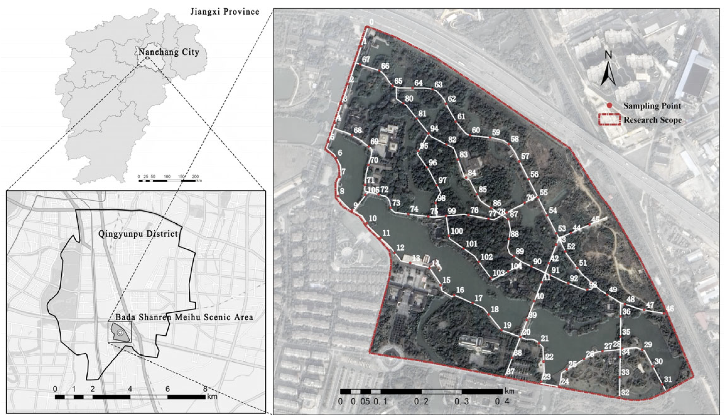
Figure 1. Research scope and sampling points.
Sustainability 17 09931 g001
Figure 2. An overview of the present study.
Sustainability 17 09931 g002
Figure 3. Example of Image depth processing results.
Sustainability 17 09931 g003
Figure 4. Example of image segmentation processing results.
Sustainability 17 09931 g004
Figure 5. Example of image color extraction processing results.
Sustainability 17 09931 g005
Figure 6. Scatter plot of predicted values vs. actual values for each model.
Sustainability 17 09931 g006
Figure 7. (a) Importance of the Indicator (b) Feature contribution in the model (top 10).
Sustainability 17 09931 g007
Figure 8. SHAP dependency graph.
Sustainability 17 09931 g008
Figure 9. Landscape preference and spatial distribution of the top four ranking indicators.
Sustainability 17 09931 g009
Figure 10. The correlation between objective indicators and landscape preferences.
Sustainability 17 09931 g010
Figure 11. The SHAP contribution of each feature in the RF model to different preference categories.
Sustainability 17 09931 g011
Figure 12. SHAP Waterfall Diagram of Sample No. 35.
Sustainability 17 09931 g012
Table 1. The demographic characteristics of 62 participants.
Demographic CharacteristicVariablesStatistics
Gender (%)Male2743.55%
Female3556.45%
Age (%)<1858.06%
18—242641.94%
25—301524.19%
31—401016.13%
41—5046.45%
51—6023.23%
>6000.00%
Educational level (%)Junior high school and below812.90%
High school1219.35%
College (bachelor’s degree)2540.32%
Master’s degree and above1727.42%
Table 2. Selection of objective indicators.
DimensionMeaningIndicatorIndicator Description
Environmental FeaturesCharacteristics of Sufficient Natural ComponentsNaturalnessProportion of natural elements (e.g., Plants, lawns, water bodies, rocks, mountains, etc.)
Naturalness = arctan([Natural Elements]/[Gray Infrastructure])
Characteristics of Wildness and Non-contactWildnessRatio of flora to the arctangent of lawns plus all non-natural elements (including gray infrastructure and other artificial facilities)
Wildness = arctan([Flora]/([Lawns] + [Non-natural Elements]))
Degree of Human Intervention in the EnvironmentArtificialnessProportion of artificial facility elements (e.g., buildings, seats, street lamps, signs, rain shelters, flower pots, outdoor flooring, sculptures, etc.)
Characteristics of Sufficient Green SpaceGreen View Index (GVI)Sum of the area proportion of all green components (trees, grass, flora)
Characteristics of Sufficient Water AreasWater View Index (WVI)Proportion of rivers, lakes, and water bodies
Spatial FeaturesCharacteristics of Free ActivityFreedomSum of the area proportions of free activity spaces (lawns, soil, ground, outdoor surfaces)
Characteristics of OpennessOpennessDistance of objects in the image from the viewpoint; image bit depth
Characteristics of Spatial HarmonyCoordinationDegree of coordination between artificial and natural elements
Coordination = (Natural Elements × Non-natural Elements)/(Natural Elements + Non-natural Elements)2
Characteristics of Sufficient Air SpaceSky View Index (SVI)Proportion of sky area in a view
Characteristics of Sufficient BuildingsBuilding View Index (BVI)Proportion of building area (houses, buildings, etc.)
Color FeatureHueH_RedColors with hue in the ranges (0,30) for bright red and (330,360) for dark red in the HSV color system
H_OrangeColors with hue in the range (30,60) in the HSV color system
H_YellowColors with hue in the range (60,90) in the HSV color system
H_GreenColors with hue in the range (90,150) in the HSV color system
H_CyanColors with hue in the range (150,210) in the HSV color system
H_BlueColors with hue in the range (210,270) in the HSV color system
H_PurpleColors with hue in the range (270,330) in the HSV color system
SaturationS_HighColors with saturation in the range (0.67,1) in the HSV color system
S_MediumColors with saturation in the range (0.33,0.67) in the HSV color system
S_LowColors with saturation in the range (0,0.33) in the HSV color system
ValueV_HighColors with value in the range (0.67,1) in the HSV color system
V_MediumColors with value in the range (0.33,0.67) in the HSV color system
V_LowColors with value in the range (0,0.33) in the HSV color system
Rich and varied colorsColor_RichnessThe differences and variations between the red, green, and blue channels in the image represent the degree of color variation
The complexity and uncertainty of visual objectsVisual_EntropyMeasures the complexity of the image by the frequency of different brightness (grayscale) values appearing
Table 3. Model performance status.
ModelMAEMSERMSER2Optimal Parameter
Decision Tree18.2542525.046922.91390.7628‘max_depth’: 3
Random Forest13.6175276.478616.62760.8751‘max_depth’: 6, ‘n_estimators’: 100
SVM23.1663845.041129.06960.6183‘C’: 1, ‘gamma’: ‘scale’, ‘kernel’: ‘linear’
Linear Regression24.1837925.096130.41540.5821
KNN27.62651105.884033.25480.5005n_neighbors’: 7
XGBoost16.3487418.322520.45290.8110‘learning_rate’: 0.05, ‘max_depth’: 3, ‘n_estimators’: 100
Table 4. The correlation between objective indicators and landscape preferences.
Objective IndicatorsMeanS.D.MinMaxElo Score
ρ p
Naturalness0.92310.38330.01921.57080.156 **0.001
Wildness0.73860.34340.00001.57030.117 *0.015
Artificialness0.34030.19370.00000.9811−0.23 **0
GVI0.45790.22100.00280.9995−0.136 **0.005
WVI0.02890.06720.00000.37260.527 **0
Freedom0.24280.14060.00000.71070.0060.895
Openness12.468914.46791.569375.21330.261 **0
Coordination0.18710.07080.00000.2500−0.0280.561
SVI0.16860.13210.00000.50060.399 **0
BVI0.12870.17450.00000.9810−0.147 **0.002
H_Red0.18930.08640.01230.5856−0.050.299
H_Orange0.27690.11950.02430.7296−0.0310.528
H_Yellow0.18350.09240.01540.6058−0.0010.982
H_Green0.09130.06720.00220.6596−0.115 *0.018
H_Cyan0.08980.08470.00200.5876−0.0650.179
H_Blue0.21830.13570.00720.64110.251 **0
H_Purple0.02460.02000.00130.1295−0.129 **0.008
S_Low0.75350.13060.31510.97990.0250.601
S_Medium0.20920.10550.01720.5316−0.040.413
S_High0.03730.03220.00070.18670.0190.699
V_Low0.26840.09640.02570.6618−0.105 *0.03
V_Medium0.40630.09100.12980.7242−0.202 **0
V_High0.32530.12110.05650.75410.245 **0
Color_Richness0.11980.03540.03660.22540.0310.519
Visual_Entropy7.59790.23426.71557.9343−0.12 *0.014
p < 0.05 *, p < 0.01 **.
Disclaimer/Publisher’s Note: The statements, opinions and data contained in all publications are solely those of the individual author(s) and contributor(s) and not of MDPI and/or the editor(s). MDPI and/or the editor(s) disclaim responsibility for any injury to people or property resulting from any ideas, methods, instructions or products referred to in the content.