Abstract
Efficient utilization of sustainable energy is imperative for supporting the globally escalating electricity demand. Because the unstable wind energy makes the wind power access challenging for power systems, the wind power forecasting becomes the critical part of the power dispatch. In this paper, a short-term wind power forecasting approach based on model configuration optimization via prequential-cross cooperative validation estimation (PCCVE) is proposed. It enables the hybrid ANN including the convolutional neural network, bidirectional long short-term memory network, and multi-head attention mechanism (CNN-BiLSTM-MHA) to better construct the wind speed–power mapping relationship for improving forecasting performance. Firstly, the box-plot local detection–correction combining the spatial–temporal optimal-weighted fuzzy clustering and the sliding window connected box-plot is proposed to reasonably detect and correct local outlier wind speed points. It prevents CNN-BiLSTM-MHA from being interfered with local outlier wind speed points. Secondly, PCCVE based on the prequential-validation estimation and cross-validation estimation is proposed to more accurately give the estimated error of CNN-BiLSTM-MHA, thus better assisting the optimization of the values of CNN-BiLSTM-MHA’s hyperparameters. It enables CNN-BiLSTM-MHA to efficiently construct the wind speed–power mapping relationship. By comparing different approaches on the actual wind farm dataset, the effectiveness and advantages of the proposed approach are demonstrated.
1. Introduction
In recent decades, to solve the increasingly serious energy shortage and environmental pollution, global energy use is shifting away from fossil fuels to sustainable energies, including wind, solar, nuclear, hydropower, and geothermal energy [1]. Among them, wind energy is more low-carbon, more economical, and more extensive, which has attracted more attention and development [2]. According to the statistics released by the World Wind Energy Association, in 2024, the total installed capacity of wind turbines in the world has reached 1174 GW, 121 GW more than that in 2023 [3]. However, wind energy is a kind of unstable energy with fluctuation and intermittence, which makes large-scale wind power access bring great challenges to the stable operation of the power system [4]. To timely and reasonably dispatch wind power to ensure the stable operation of the power system, the development and application of short-term (30 min to 6 h in advance) wind power forecasting is very important [5].
With the development of computer science, many artificial neural network models (ANNs), such as the back propagation neural network [6], long-term and short-term memory network [7], and convolutional neural network [8], are proposed and widely used in short-term wind power forecasting. Compared with the traditional physical models [9,10] and statistical models [11,12], ANN is better at constructing the complex wind speed–power mapping relationship to provide more accurate short-term wind power forecasting. To enable ANN to better construct the wind speed–power mapping relationship, model configuration optimization and data preprocessing are extensively studied [13].
Model configuration optimization aims at optimizing the values of hyperparameters of ANN to efficiently construct the wind speed–power mapping relationship [14]. Usually, the error estimation method is used to give the estimated error of ANN. According to the estimated error, the hyperparameters of ANN are reconfigured with better values by the optimization algorithm [15]. At present, there are two commonly used error estimation methods: (a) prequential-validation estimation (PVE) [16] and (b) cross-validation estimation (CVE) [17]. Both PVE and CVE cut the time series (such as the wind speed series) into several equal-size and orderly subsets for multiple operations. Each operation is to select some subsets to train and verify ANN in a certain way to produce a verification error. After multiple operations, verification errors are averaged as the estimated error. For the error estimation method, the less the estimated error deviates from the actual error of ANN obtained in practical application, the more accurate it is. However, the first few operations of PVE have the data under-utilization problem [18], which makes the estimated error deviate from the actual error and limits the accuracy of PVE. Furthermore, most operations of CVE have the data leakage problem [19], which also makes the estimated error deviate from the actual error and limits the accuracy of CVE. Even worse, inaccurate PVE and CVE sometimes mislead the optimization algorithm to finally configure hyperparameters with suboptimal value, which limits ANN from providing better wind power forecasting. Compared with previous researches that only blindly used PVE or CVE, Ref. [20] reasonably made the comprehensive use of PVE and CVE. Specifically, Ref. [20] studied the deviation distance characteristic of PVE and CVE, which finds that if the non-stationary degree of the time series is higher, estimated errors given by PVE and CVE tend to be closer to and further away from the actual error, respectively; if the non-stationary degree is lower, estimated errors given by PVE and CVE tend to be further away and closer to the actual error, respectively. So, Ref. [20] used PVE and CVE when the non-stationary degree is high and low, respectively. However, the essence of this comprehensive use of PVE and CVE is a simple selection of PVE and CVE, and its accuracy is still not high enough. To our knowledge, more and more deviation characteristics of PVE and CVE are studied, such as the deviation direction characteristic [21,22]. It finds that estimated errors given by PVE and CVE tend to be higher and lower than the actual error, respectively. Therefore, deeply studying the deviation characteristics of PVE and CVE to realize more accurate comprehensive use of PVE and CVE is the first motivation of this paper.
Data preprocessing often focuses on preventing outlier wind speed points from interfering with the construction of the wind speed–power mapping relationship [23]. Box-plot [24], as a popular statistical-based detection method with good effect, is often used to preprocess outlier data points. Compared with distance/density-based detection methods [25] that rely on complex abstract calculation, the box-plot uses concise statistical quantiles to perform detection, which is more interpretable and reliable. In addition, the z-score is also a statistical-based detection method, but it relies on statistical standard deviation and can only be applied to data that obey normal distribution [26]. Better than the z-score, the box-plot has no requirement for data distribution, which is more universal. Since wind speed data usually obey non-strict normal distribution, the box-plot is more used than the z-score to preprocess outlier wind speed points. For example, Ref. [27] adopted the traditional box-plot detection, which uses the quartiles of all wind speed points to construct box-plot boundaries, thus identifying wind speed points exceeding box-plot boundaries as outlier wind speed points. However, the outlier detection strategy [28] points out that if global time data points are used as the detection context, the global outlier points are detected; if local time data points are used as the detection context, the local outlier points are detected. Obviously, the traditional box-plot detection only identifies global outlier wind speed points but ignores local outlier wind speed points. To identify local outlier points, Ref. [29] used the sliding window with the relatively small width to capture local time data points. However, the sliding window only captures and provides few local time data points, which makes it difficult for the box-plot to reasonably detect local outlier points. This is because when local time data points are few, they contain fewer reasonable time data points, which hardly ensures their quartiles are accurate enough under the influence of local outlier wind speed points. This further makes box-plot boundaries not accurate enough to reasonably detect these local outlier points. Therefore, how to capture and input a sufficient number of reasonable local wind speed points to the box-plot to more reasonably detect and correct local outlier wind speed points is the second motivation of this paper.
Inspired by the above work, a short-term wind power forecasting approach based on model configuration optimization via prequential-cross cooperative validation estimation (PCCVE) is proposed. Firstly, the historical wind speed series from the SCADA system of the wind turbine is provided. Secondly, in the data preprocessing of historical wind speed series, the box-plot local detection–correction combining the spatial–temporal optimal-weighted fuzzy clustering and the sliding window connected box-plot is proposed to reasonably detect and correct local outlier wind speed points to produce the available historical wind speed series. Spatial–temporal optimal-weighted fuzzy clustering, which adopts the traditional similarity objective function, the novel balance objective function, and non-dominated sorting [30], is proposed to effectively transform the historical wind speed series into several clusters of similar wind speed segments, thus further providing them to the sliding window connected box-plot. Then, in the model configuration optimization of the hybrid deep ANN including the convolutional neural network, bidirectional long short-term memory network, and multi-head attention mechanism (CNN-BiLSTM-MHA) [31], and PCCVE based on PVE and CVE is proposed to more accurately give the estimated error of CNN-BiLSTM-MHA, thus better assisting the dual fitness particle swarm optimization [32] to optimize the values of CNN-BiLSTM-MHA’s hyperparameters. Finally, CNN-BiLSTM-MHA with the optimal values of main hyperparameters is trained with the available historical wind speed series, and the real-time wind speed series is input to the trained CNN-BiLSTM-MHA to receive the forecasted wind power series.
The innovations of this approach are as follows:
(1) Prequential-cross cooperative validation estimation (PCCVE) based on PVE and CVE is proposed for the first time to more accurately give the estimated error of ANN. By synthesizing the deviation direction and distance characteristics of PVE and CVE, the relative position relationship of the actual error of ANN to the estimated errors given by PVE and CVE is confirmed. This relative position relationship indicates that in the value space, the actual error of ANN tends to be between the estimation errors given by PVE and CVE, and it further tends to be closer to one of those two estimation errors due to the influence of the non-stationary degree of the time series used in PVE and CVE. According to this relative position relationship, the estimated errors given by PVE and CVE can be used to give a better estimated error that is closer to the actual error of ANN. Therefore, in model configuration optimization, PCCVE is more effective than PVE and CVE at guiding the optimization algorithm to finally configure hyperparameters with optimal values instead of suboptimal values, which promotes ANN to provide better wind power forecasting.
(2) Box-plot local detection–correction adopting the spatial–temporal optimal-weighted fuzzy clustering, the sliding window, and the box-plot is proposed for the first time to more reasonably detect and correct local outlier wind speed points. Due to the regular behaviors of wind [33], the clustering is used to transform the wind speed series into similar wind speed segments. When the sliding window is slid on similar wind speed segments to capture and input local wind speed points to the box-plot, local outlier wind speed points are more reasonably detected, because the number of local wind speed points captured by each sliding on similar wind speed segments is significantly more than that captured by each sliding on the wind speed series. Accordingly, there is a larger number of reasonable local wind speed points to resist the influence of local outlier wind speed points on the accuracy of quartiles, which further makes box-plot boundaries accurate enough.
(3) Due to the cosine measure being more sensitive to time series data than the Euclidean measure, the traditional similarity objective function based on these two measures in the spatial–temporal clustering [34] often causes the cosine measure to have an overly large weight, which further makes similar wind speed segments have overly significant temporal variation similarity and insignificant spatial position similarity, that is, insignificant spatial–temporal similarity. Therefore, the spatial–temporal optimal-weighted fuzzy clustering, which uses the novel balance objective function besides the traditional similarity objective function, is proposed for the first time to produce similar wind speed segments with more significant spatial–temporal similarity. The balance objective function is designed to evaluate the balance degree of temporal variation similarity and spatial position similarity under current weights, which further guides non-dominated sorting to select more appropriate weights for cosine measure and Euclidean measure, thus balancing the improvements of temporal variation similarity and spatial position similarity.
2. Proposed Approach
The flowchart of the proposed approach can be illustrated in Figure 1, and the procedure can be described as follows:
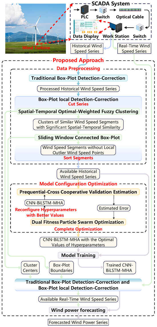
Figure 1.
Flowchart of the proposed approach.
Step I: Obtain the historical wind speed series that comes from the SCADA system of the local wind turbine.
Step II: Apply the traditional box-plot detection–correction [27] and the proposed box-plot local detection–correction to the historical wind speed series in turn, which deals with the global outlier wind speed points and the local outlier wind speed points, respectively, thus getting the available historical wind speed series.
Step III: Configure the hyperparameters of the CNN-BiLSTM-MHA with random values.
Step IV: Utilize the proposed prequential-cross cooperative validation estimation to train and validate the CNN-BiLSTM-MHA with the available historical wind speed series to give the estimated error of the CNN-BiLSTM-MHA.
Step V: Use the estimated error to guide the dual fitness particle swarm optimization [32] to reconfigure the hyperparameters of the CNN-BiLSTM-MHA with better values that may further reduce the estimated error.
Step VI: Repeat Step IV and Step V until the maximum number of optimizations is reached. The optimal values of hyperparameters that minimize the estimated error of the CNN-BiLSTM-MHA are obtained. The CNN-BiLSTM-MHA with the optimal values of hyperparameters is finally trained with the whole available historical wind speed series to produce the trained CNN-BiLSTM-MHA.
Step VII: Perform the same detection–corrections as in Step II to the real-time wind speed series in turn to produce the available real-time wind speed series. The box-plot boundaries and cluster centers of the detection–corrections in this step do not need to be calculated but come from Step II.
Step VIII: Input the real-time wind speed series that comes from the SCADA system of the local wind turbine to the trained CNN-BiLSTM-MHA to output the forecasted wind power series.
2.1. Data Preprocessing Based on Box-Plot Local Detection–Correction
The spatial–temporal optimal-weighted fuzzy clustering and the box-plot local detection–correction are described in the following two parts, respectively:
2.1.1. Spatial–Temporal Optimal-Weighted Fuzzy Clustering
The historical wind speed series is cut into M wind speed segments with equal width and chronological order. Define the jth wind speed segment as , , the number of clusters as K, the kth clustering center as , , the weights of Euclidean and cosine measures as w and , respectively, , the spatial–temporal fuzzy clustering based on Euclidean measure, cosine measure, and fuzzy c-means clustering, which can be described as follows:
Step I: Randomly initialize the spatial position membership degree and the temporal variation membership degree of to , , , , .
Step II: Calculate the spatial–temporal membership degree by
Step III: Update the cluster center by
Step IV: Update and by
where m is the fuzzy coefficient, and and are Euclidean measure and cosine measure in [34], respectively.
Step V: Repeat Step II to Step V until the maximum number of iterations is reached.
Step VI: Divide to the th cluster if is the largest in , .
Step VII: Output K clusters of similar wind speed segments.
To ensure similar wind speed segments have significant spatial–temporal similarity, w needs to be optimized based on the similarity objective function and the novel balance objective function . Like the traditional similarity objective function in [34], also makes w optimized to improve the spatial–temporal similarity of similar wind speed segments in the same cluster, which is designed as follows:
where the smaller , the more improvement of spatial–temporal similarity. Because is more sensitive to time series data, such as wind speed segments, the greater is than w, the smaller . However, it leads to the improvement of spatial–temporal similarity realized by overly improving temporal variation similarity and slightly improving spatial position similarity, which further makes similar wind speed segments have overly significant temporal variation similarity and insignificant spatial position similarity, that is, insignificant spatial–temporal similarity.
Therefore, is used to balance the improvements of temporal variation similarity and spatial position similarity, which is designed as follows:
where the smaller , the more balanced improvements of temporal variation similarity and spatial position similarity. The closer w and are, the smaller is.
Obviously, it is conflicting to reduce and at the same time, which indicates that the optimization of w is a multi-objective optimization problem. Well-known, non-dominated sorting genetic algorithm II, as a multi-objective optimization method composed of genetic algorithm and non-dominated sorting [29], is widely used. However, the value range of w is relatively small, which makes the use of the genetic algorithm overqualified. Therefore, grid search is used to replace the genetic algorithm, and its combination with non-dominated sorting is used to optimize w. The spatial–temporal optimal-weighted fuzzy clustering can be described as follows:
Step I: Use grid search to select P different values with D decimal places from (0,1) as weights , .
Step II: Apply the spatial–temporal fuzzy clustering under each weight of to receive the corresponding .
Step III: Utilize and non-dominant sorting to sort and receive the pareto front of non-dominated weights, as shown in Figure 2.
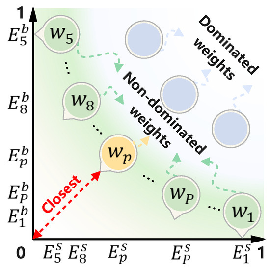
Figure 2.
Pareto front of non-dominated weights.
In Figure 2, the non-dominated weight on the pareto front, which is closest to , is selected as the best weight, . Because and of are moderate in and , respectively, it indicates has makes the compromise between improving spatial–temporal similarity and balancing spatial–temporal similarity, which enables K clusters of similar wind speed segments to have not only significant temporal variation similarity but also significant spatial position similarity, that is, significant spatial–temporal similarity.
Step IV: Output K clusters of similar wind speed segments obtained under .
2.1.2. Box-Plot Local Detection–Correction
Suppose there is a periodic time data series, which is shown in Figure 3.
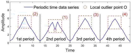
Figure 3.
Periodic time data series.
In Figure 3, there is the local outlier point O with the value of in the 2nd period. When the sliding window is slid at area (1), local time data points , , , , are captured and input to the box-plot. The lower quartile , upper quartile , and quartile distance of those local time data points are 3.69, 5.05, and 1.36, respectively. By and , box-plot boundaries and are calculated as 3.01 and 7.1, respectively. However, is lower than O, which makes O not detected. The reason for the detection failure is that so few local time data points are captured that each of them significantly influences the accuracy of quartiles and box-plot boundaries. Among them, O is overly far below other points, which makes too small, too big, and too low. Generally, periods in the periodic time data series are similar, which makes local outlier points in one period more reasonably detected by referring to a sufficient number of reasonable local time data points in other periods. When local time data points in area (1) are input to the box-plot together with local time data points , , , , in area (2), local time data points , , , , in area (3), and local time data points , , , , in area (4), , , and are 3.91, 5.13, and 1.22, respectively. and are constructed as 3.3 and 6.96, respectively. Obviously, the use of local time data points in areas (2), (3), and (4) resists the influence of O on the accuracy of quartiles and box-plot boundaries, which makes bigger than , smaller than , and higher than . Importantly, is higher than O, which makes O detected. Like similar periods in the periodic time data series, there are similar wind speed segments in the historical wind speed series due to the regular behaviors of wind. Generally, the clustering is used to identify similar wind speed segments and put them into the same cluster. In the same cluster, local outlier wind speed points in one wind speed segment can also be more reasonably detected by referring to a sufficient number of reasonable local wind speed points in other wind speed segments.
Define the local wind speed point at time i of the zth wind speed segment in the kth cluster as , , the width of the wind speed segment as W, , the number of wind speed segments in the kth cluster as , and the box-plot local detection–correction can be illustrated in Figure 4, and the procedure can be described as follows:
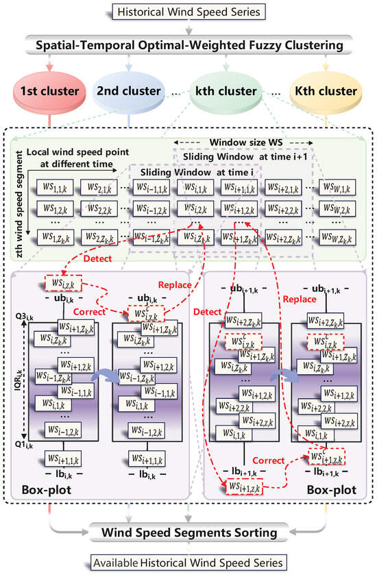
Figure 4.
Structure of the box-plot local detection–correction (window size = 3).
Step I: Perform the spatial–temporal optimal-weighted fuzzy clustering to the historical wind speed series to receive K clusters of similar wind speed segments. Set and .
Step II: Apply the sliding window at time i of the k th cluster to capture and input local wind speed points not only , , , but also , , , …, , , of similar wind speed segments to the box-plot.
Step III: Use the lower quartile , the upper quartile , and the quartile distance of local wind speed points to construct the box-plot upper boundary and box-plot lower boundary by and .
Step IV: Utilize and to detect and correct each local wind speed point in turn. If the local wind speed point is higher than or lower than , it is detected as a local outlier wind speed point, and it is further moved down to or up to to produce the corrected local wind speed point . Otherwise, it is detected as a reasonable local wind speed point.
Step V: Set and repeat Step II to Step IV until .
Step VI: Set and . Repeat Step II to Step V until .
Step VII: Use the chronological order in Section 2.1.1. to sort all wind speed segments that have no local outlier wind speed points to produce the available historical wind speed series.
2.2. Model Configuration Optimization Based on Prequential-Cross Cooperative Validation Estimation
PCCVE and CNN-BiLSTM-MHA are described in the following two parts, respectively:
2.2.1. Prequential-Cross Cooperative Validation Estimation
Both PVE and CVE cut the time series into several equal-size and orderly subsets for multiple operations. Each operation is to select some subsets to train and verify ANN in a certain way to produce a verification error. After multiple operations, verification errors are averaged as the estimated error of ANN.
For PVE, the subsets used for training are strictly earlier than the subset used for verification, which follows the forecasting logic of “forecasting the future data with the historical data”. However, in the first few operations, only a few subsets are used for training, which easily leads to the data under-utilization problem [18], resulting in verification errors of ANN being overly high. These verification errors further make the estimated error tend to deviate from and be higher than the actual error of ANN [21], which is the deviation direction characteristic of PVE.
Different with PVE, CVE makes full use of subsets to avoid the data under-utilization problem to some extent. In each operation, one subset is used for verification, and other subsets are used for training. However, in most operations, subsets used for training are later than subsets used for verification, which does not follow the forecasting logic and easily leads to the data leakage problem [19], resulting in verification errors of ANN being overly low. These verification errors further make estimated error tend to deviate from and be lower than [22], which is the deviation direction characteristic of CVE.
Importantly, PVE and CVE are sensitive to the non-stationarity degree of the time series [20]. When the non-stationarity degree is low, the consistency between historical data and future data is strong, which makes the influence of the data leakage problem on CVE less. In addition, unlike PVE, CVE is not influenced by the data under-utilization problem. Therefore, compared with , deviates less from . On the contrary, when the non-stationarity degree is high, the data leakage problem has more influence on CVE. Unlike CVE, PVE is not influenced by the data leakage problem. Furthermore, the influence of the data under-utilization problem on PVE is limited. Therefore, compared with , deviates less from . In summary, if the non-stationary degree of the time series becomes higher, and tend to be closer to and further away from , respectively; if the non-stationary degree becomes lower, and tend to be further away and closer to , respectively. This is the deviation distance characteristic of PVE and CVE.
By synthesizing the deviation direction characteristics of PVE and CVE, the relative position relationship of to and in the value space is pointed out. It finds that tends to be higher than and lower than , that is, between and . By further introducing the deviation distance characteristics of PVE and CVE, this relative position relationship is improved. It further finds that if the non-stationary degree , of the time series becomes higher, tends to be closer to than , and if becomes lower, tends to be closer to than , which is illustrated in Figure 5.
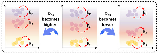
Figure 5.
Relative position relationship of the actual error of ANN to the estimated error given by PVE and estimated error given by CVE in the value space ( is the non-stationarity degree of the time series).
According to this relative position relationship, can be dynamically approximated by , which is illustrated in Figure 6.
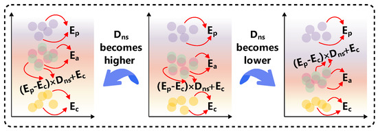
Figure 6.
Approximate value of in the value space ( and are estimated errors given by PVE and CVE, is the actual error of ANN, and is the non-stationarity degree of the time series).
In Figure 6, it can be seen that is also between and , like . If becomes higher, tends to be closer to than , like ; if becomes lower, tends to be closer to than , like . Compared with and , deviates less from . Therefore, it is feasible for PVE and CVE to cooperate to more accurately give as the estimated error of ANN.
Define the nth subset of the available historical wind speed series as , , and the prequential-cross cooperative validation estimation based on PVE and CVE can be illustrated in Figure 7, and the procedure can be described as follows:
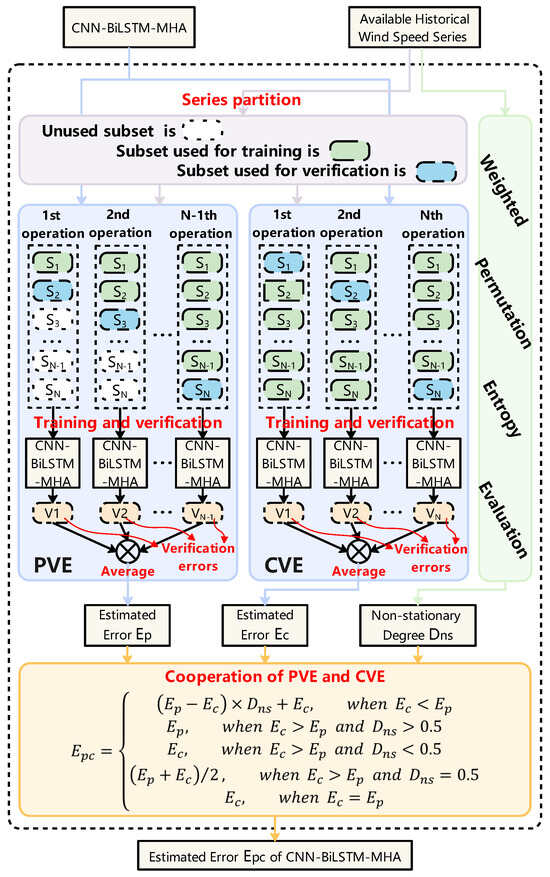
Figure 7.
Structure of prequential-cross cooperative validation estimation.
Step I: Partition the available historical wind speed series into N equal-size and orderly subsets . Set and .
Step II: Train CNN-BiLSTM-MHA with and verify CNN-BiLSTM-MHA with to produce the verification error .
Step III: Set and repeat Step II until .
Step IV: Average as the estimated error given by PVE.
Step V: Train CNN-BiLSTM-MHA with and . Verify CNN-BiLSTM-MHA with to produce the verification error .
Step VI: Set and repeat Step V until .
Step VII: Average as the estimated error given by CVE.
Step VIII: Use the weighted permutation entropy evaluation [35] to evaluate the available historical wind speed series to receive the non-stationary degree , .
Step IX: Use , , and to produce the estimated error of CNN-BiLSTM-MHA. In most cases of < , = , due to the interference of the random error, < is sometimes not satisfied. In a few cases of > , according to the deviation distance characteristics of PVE and CVE [20], if > , PVE is considered more accurate than CVE, so ; if , CVE is considered more accurate than PVE, so ; and if , PVE and CVE are considered equally accurate, so . In rare cases of , .
Compared with PVE and CVE, PCCVE more accurately estimates the quality of values of hyperparameters. That is to say, when PCCVE is used to guide the optimization algorithm, the optimal value is easier to select, which ensures ANN accurately forecasts wind power.
Suppose there are two sets of values of hyperparameters, and , which are optimal and suboptimal, respectively. The actual errors of ANN under and are and , respectively, and < . When PVE is used to estimate the quality of and , the estimated errors of and are and , respectively. Due to the accuracy of PVE being insufficient, the situation of > appears with high probability. If so, is configured to the hyperparameters of ANN. is obtained and means that ANN inaccurately forecasts wind power. Like PVE, CVE faces the above situation. When PCCVE is used to estimate the quality of and , the estimated errors of and are and , respectively. Due to the accuracy of PCCVE being relatively sufficient, the situation of < appears with high probability. If so, is configured to the hyperparameters of ANN. is obtained and means that ANN accurately forecasts wind power.
According to given by PCCVE, the dual fitness particle swarm optimization [32] is used to reconfigure the hyperparameters of the CNN-BiLSTM-MHA with better values that may further reduce . Until the maximum number of optimizations is reached, the CNN-BiLSTM-MHA with the optimal values of hyperparameters is finally trained with the whole available historical wind speed series. The real-time wind speed series is further input to the trained CNN-BiLSTM-MHA to output the forecasted wind power series.
2.2.2. CNN-BiLSTM-MHA
CNN-BiLSTM-MHA, as a hybrid deep ANN with a well-developed ability of feature extraction, is used to construct the wind speed–power mapping relationship and forecast wind power. Define the ith input and ith output of CNN-BiLSTM-MHA in the training process as available historical wind speed points and the available historical wind power point , respectively, the lag step as g, and the forecast horizon as h, and the training process of CNN-BiLSTM-MHA can be illustrated in Figure 8.
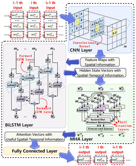
Figure 8.
Training process of CNN-BiLSTM-MHA.
In Figure 8, the CNN layer is used to extract local features on small regions of with the convolutional kernel, which outputs the feature maps with spatial information. The BiLSTM layer is used to extract the contextual features of the feature map from both forward and reverse directions with the forward LSTM layer and the backward LSTM layer, which outputs hidden state vectors with spatial–temporal information. The MHA layer is used to correlate all the features and positional information of hidden state vectors with through multiple self-attention layers, which outputs attention vectors with more important spatial–temporal information. The fully connected layer is used to linearly transform attention vectors to approximate to construct the wind speed–power mapping relationship.
When the trained CNN-BiLSTM-MHA is in the verification process, the jth input is available historical wind speed points , and the jth output is the forecasted wind power point of the available historical wind power point . When the trained CNN-BiLSTM-MHA is in the testing process, the zth input is real-time wind speed points , and the zth output is the forecasted wind power point of the future wind power at time .
3. Application
The proposed approach is built using MATLAB version R2023a. All calculations are performed on the computer with the hardware device of Intel(R) Xeon(R) Silver 4210 CPU (20 cores, 40 threads, and 2.20 GHz base frequency), as well as the Windows 10 operating system. To be mentioned, the proposed approach contains a large number of loop operations, and each operation includes the training and verification of a deep learning network, which is relatively time-consuming. Since there is no information dependence among operations, the parallel computing toolbox of MATLAB is used to execute operations on 20 cores in parallel to accelerate the running of the proposed approach.
3.1. Datasets Description
The layout of the kelmarsh wind farm in the United Kingdom is shown in Figure 9. In the wind farm, the actual wind dataset of the 6th wind turbine (rated capacity is 2050 kW) is collected by the SCADA system (sampling from 1 January 2020 to 31 December 2021 with a 10 min interval) and used for experiments.
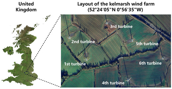
Figure 9.
Layout of the kelmarsh wind farm in the United Kingdom.
In the dataset, there are wind speed points and wind power points, which are, respectively, processed by the min–max normalization method:
where is the normalized data point, x is the original data point, and and are the maximum data points and minimum data points, respectively. The dataset is resampled with the 1 h interval and then divided into training/validation set and testing set. These two sets contain 8708 and 8669 normalized wind speed–power points, respectively.
3.2. Evaluation Indices
Normalized root mean square error (NRMSE) and normalized mean absolute error (NMAE) are utilized.
where and are the forecasted and actual wind power. L is the length of the actual wind power series. is the rated capacity of the wind turbine. The smaller NRMSE and NMAE, the better the forecasting performance.
4. Experiments and Analysis
4.1. Effectiveness Analysis of Spatial–Temporal Optimal-Weighted Fuzzy Clustering
To verify the spatial–temporal optimal-weighted fuzzy clustering (SOFC), optimally weighted Euclidean measures and cosine measures to enable similar wind speed segments to have good spatial–temporal similarity, clusters output by the spatial–temporal empirical-weighted k-means clustering (EKC) [34], and SOFC are compared. The clusters output by EKC are shown in Figure 10.
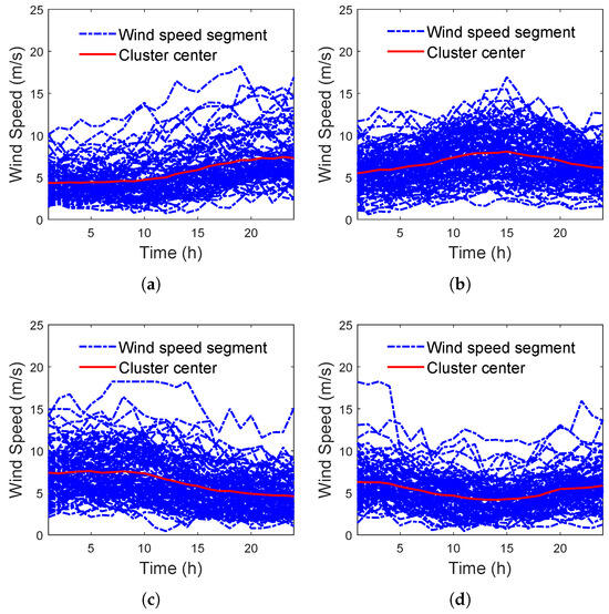
Figure 10.
Clusters output by EKC. (a) The 1st cluster output by EKC. (b) The 2nd cluster output by EKC. (c) The 3rd cluster output by EKC. (d) The 4th cluster output by EKC.
In Figure 10, it can be clearly seen that similar wind speed segments in the same cluster have similar curve shapes but different curve heights, which indicates that similar wind speed segments output by EKC have significant temporal variation similarity but insignificant spatial position similarity, that is, insignificant spatial–temporal similarity.
The pareto front of weights of SOFC is shown in Figure 11.
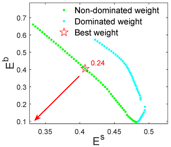
Figure 11.
Pareto front of weights of SOFC.
The clusters output by SOFC under are shown in Figure 12.
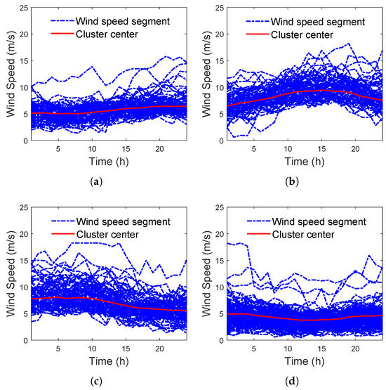
Figure 12.
Clusters output by SOFC. (a) The 1st cluster output by SOFC. (b) The 2nd cluster output by SOFC. (c) The 3rd cluster output by SOFC. (d) The 4th cluster output by SOFC.
In Figure 12, it can be clearly seen that similar wind speed segments in the same cluster have not only close curve heights but also similar curve shapes, which indicates that similar wind speed segments output by SOFC have significant temporal variation similarity and significant spatial position similarity, that is, significant spatial–temporal similarity.
4.2. Effectiveness Analysis of Box-Plot Local Detection–Correction
To verify that similar wind speed segments give accurate enough quartiles, including the lower quartile , upper quartile , and quartile distance to construct box-plot boundaries, bootstrap [36] is used. Bootstrap, as a popular statistical method to estimate the point distribution characteristics by repeatedly and randomly sampling, gives the 95% confidence interval (CI) of the point distribution characteristics of the original point set. The 95% CI can be further used to reflect the accurate degree of point distribution characteristics. The 95% CIs of , , and given by different numbers of similar wind speed segments are shown in Figure 13.
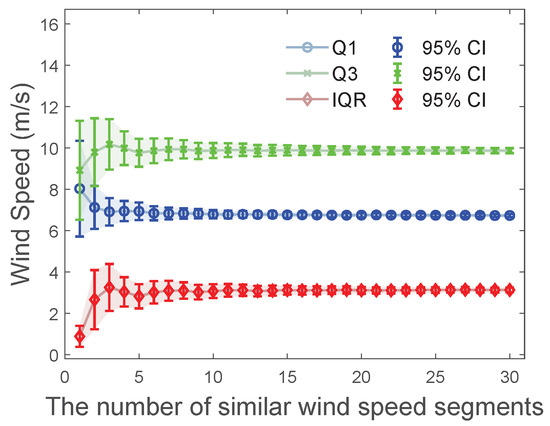
Figure 13.
The 95% CIs of , , and given by different numbers of similar wind speed segments.
In Figure 13, it can be clearly seen that the more the number of similar wind speed segments, the narrower the 95% CIs of , , and , which means , , and are more accurate. Until the number of similar wind speed series is higher than 20, the 95% CIs are no longer obviously narrow and tend to be stable, which means , , and are accurate enough.
Importantly, the number of similar wind speed segments in each cluster in SOFC is much higher than 20. It ensures that , , and are accurate enough and can be used to construct box-plot upper and lower boundaries in the sliding window connected box-plot (SWBP).
Then, the detection and correction of local outlier wind speed points by SWBP on K clusters are shown in Figure 14.
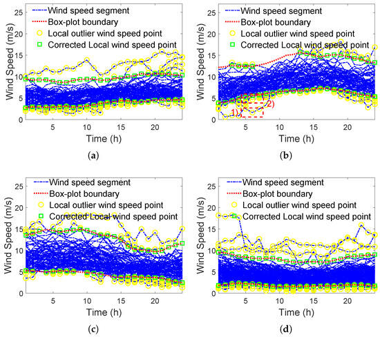
Figure 14.
Detection and correction of local outlier wind speed points by SWBP on each cluster (number of clusters ). (a) SWBP on 1st cluster. (b) SWBP on 2nd cluster. (c) SWBP on 3rd cluster. (d) SWBP on 4th cluster.
In Figure 14, box-plot upper and lower boundaries are reasonably constructed in each cluster, and they well surround similar wind speed segments that have good spatial–temporal similarity. However, local wind speed points exceeding these boundaries are inconsistent with the spatial–temporal similarity, so they are detected as local outlier wind speed points and further corrected. For example, in Figure 14b, wind speed segments follow the spatial–temporal similarity, that is, the spatial position of “Around wind speed = 9 m/s” and temporal variation of “Low to high to low”. However, local wind speed points in area (1) distribute too low and rise too slowly, which is inconsistent with the spatial–temporal similarity and exceed the box-plot low boundary. So, these local wind speed points are detected as local outlier wind speed points and further moved to the box-plot lower boundary to produce corrected local outlier wind speed points in area (2).
To intuitively illustrate the effectiveness of BLDC, the detection labels output by the z-score (Z), box-plot (B), and BLDC are compared, as shown in Figure 15. Note that the sliding window (S) is also used to assist Z and B to detect local outlier wind speed points.
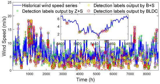
Figure 15.
Detection labels output by different detection methods.
In Figure 15, it can be clearly seen that the behaviors of the wind speed points labeled by Z+S, B+S, and BLDC are relatively abnormal to that of their neighboring points, which belong to local outlier wind speed points. This indicates that Z+S, B+S, and BLDC are all effective. However, both Z+S and B+S only observe a few neighboring points to judge whether a wind speed point should be labeled, which faces the problem that the number of normal wind speed points is insufficient to effectively highlight the local outlier wind speed points. Therefore, there are many local outlier wind speed points that are only labeled by BLDC, especially when the wind speed is low, such as between time 5400 and time 5480. This indicates BLDC is more effective than Z+S and B+S.
To further quantify the effectiveness of BLDC, the accuracy of the approaches based on different combinations of Z+S, B+S, BLDC, and TCN-LSTM (T) are compared. The forecasted wind power series of different approaches are shown in Figure 16. Note that local outlier wind speed points detected by Z and B are removed and filled by the cubic spline interpolation (I).
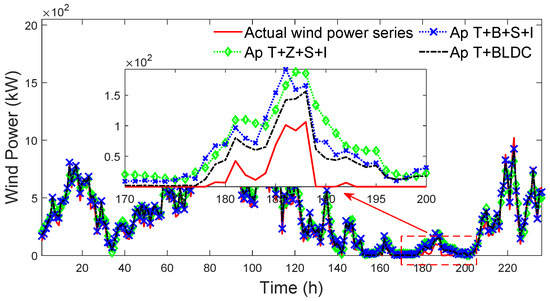
Figure 16.
Forecasted wind power series of different approaches (the values of the hyperparameters of T in different approaches are kept consistent).
In Figure 16, it can be clearly seen that the forecasted wind power series of Ap T+BLDC more approximate the actual wind power series than that of Ap T+Z+S+I and Ap T+B+S+I, especially between time 170 and time 200. The reason is that BLDC more effectively removes abnormal spatial–temporal characteristics caused by local outlier wind speed points, which enables T to better construct the wind speed–power mapping relationship to forecast wind power. The forecasting errors of different approaches are shown in Table 1.

Table 1.
Forecasting errors of different approaches.
In Table 1, it can be clearly seen that NRMSE and NMAE of Ap T+BLDC are significantly reduced compared with Ap T+Z+S+I and Ap T+B+S+I.
To verify the significance of the forecasting improvements of BLDC relative to Z+S+I and B+S+I, bootstrap is applied for significance testing. Firstly, repeated sampling with replacement is carried out from the testing set to generate many bootstrap testing sets. Then, on each bootstrap testing set, NRMSE under BLDC is used to subtract NRMSE under Z+S+I, and the difference value is recorded. Finally, a 95 % confidence interval is constructed based on the distribution of these difference values, which is [−0.93, −0.44]. Obviously, [−0.93, −0.44] is completely less than 0, which proves that the forecasting improvement of BLDC relative to Z+S+I is significant and stable. A 95 % confidence interval of the forecasting improvement of BLDC relative to B+S+I is also calculated, which is [−0.86, −0.31].
In addition, the runtimes of Z+S, B+S, and BLDC under the wind speed series with different lengths are shown in Table 2.
Table 2.
Runtimes of different detection methods.
In Table 2, it can be clearly seen that the runtimes of Z+S, B+S, and BLDC all increase with the increase in the length of wind speed series. However, the runtimes of BLDC are much longer than that of Z+S and B+S, because there is the spatial–temporal optimal-weighted fuzzy clustering in BLDC, which is relatively time-consuming.
4.3. Effectiveness Analysis of Prequential-Cross Cooperative Validation Estimation
To verify the accuracy of the prequential-cross cooperative validation estimation (PCCVE), the estimation deviations of PVE, CVE, and PCCVE are compared. However, multilayer perceptron (MLP) and elman neural network (ELMAN) need to be trained by a sufficient amount of data. So, MLP and ELMAN are sensitive to the data under-utilization problem, which easily make the estimation deviations of PVE large. Long short-term memory (LSTM) and temporal convolutional network (TCN) need to capture long-term temporal information. So, LSTM and TCN are more sensitive to the data leakage problem, which more easily make the estimation deviations of CVE large. Since the construction of PCCVE is based on PVE and CVE, the estimation deviation of PCCVE is also influenced by the type of ANN. Therefore, the estimation deviations of PVE, CVE, and PCCVE should be compared on different types of ANNs to more strictly verify the accuracy of PCCVE. The main hyperparameters of four different types of ANNs are shown in Table 3.
Table 3.
Main hyperparameters of four different types of ANNs.
The relatively effective values of these main hyperparameters are determined as = , = , = , = , = , = , and = . By traversing all combinations of the values of , , , and to configure MLP, 840 different MLPs are obtained. By defining the estimated error minus the actual error as the estimation deviation, the estimation deviations of PVE, CVE and PCCVE on 840 different MLPs are obtained. So on, the estimation deviations of PVE, CVE, and PCCVE on 840 ELMANs, 168 LSTMs, and 2688 TCNs are obtained. Violin plot [37], as a popular data visualization method, can be used to reflect the distribution differences between different data. Violin plots of estimation deviations of PVE, CVE, and PCCVE on four different types of ANNs are shown in Figure 17.
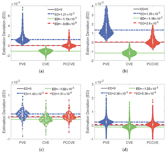
Figure 17.
Violin plots of estimation deviations of PVE, CVE, and PCCVE on four different types of ANNs (non-stationary degree = 0.475 and number of subsets N = 5). (a) Violin plots of estimation deviations of PVE, CVE and PCCVE on 840 MLPs. (b) Violin plots of estimation deviations of PVE, CVE and PCCVE on 840 ELMANs. (c) Violin plots of estimation deviations of PVE, CVE, and PCCVE on 168 LSTMs. (d) Violin plots of estimation deviations of PVE, CVE, and PCCVE on 2688 TCNs.
In Figure 17, the violin plots of estimation deviations of PVE, CVE, and PCCVE on 840 MLPs, 840 ELMANs, 168 LSTMs, and 2688 TCNs are shown in Figure 17a–d in turn. In Figure 17a, violin plots show that the estimation deviations of PVE on MLPs are mainly distributed above and far from ED = 0, around , the estimation deviations of CVE on MLPs are mainly distributed below and far from ED = 0, around , and the estimation deviations of PCCVE on MLPs are mainly distributed near ED = 0, around . Importantly, it can be clearly seen that the distribution of estimation deviations of PCCVE is relatively closer to ED = 0 than that of PVE and CVE, which indicates that is generally closer to than and . That is, PCCVE is more accurate than PVE and CVE in giving the estimated errors of MLPs. Furthermore, in Figure 17b–d, the comparison between violin plots of estimation deviations of PVE, CVE, and PCCVE also indicate that PCCVE is more accurate than PVE and CVE in giving the estimated errors of ELMANs, LSTMs, and TCNs.
To verify the improvements of the PVE, CVE, and PCCVE to the model performance, the accuracy of the approaches based on different combinations of PVE, CVE, PCCVE, the dual fitness particle swarm optimization (D), and TCN-LSTM (T) are compared. The forecasted wind power series of different approaches are shown in Figure 18.
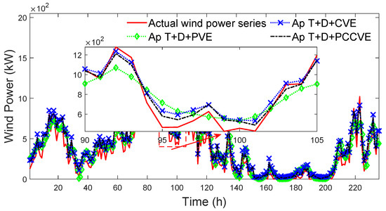
Figure 18.
Forecasted wind power series of different approaches.
In Figure 18, it can be clearly seen that the forecasted wind power series of Ap T+D+PCCVE more approximate the actual wind power series than that of Ap T+D+PVE and Ap T+D+CVE, especially between time 90 and time 105. The forecasting errors of different approaches are shown in Table 4.
Table 4.
Forecasting errors of different approaches.
In Table 4, it can be clearly seen that NRMSE and NMAE of Ap T+D+PCCVE are significantly reduced compared with Ap T+D+PVE and Ap T+D+CVE. The main reason is that the hyperparameters of T in Ap T+D+PCCVE are better configured. In the training result of Ap T+D+PCCVE, T is configured with , and the NRMSE of T estimated by PCCVE is 4.12. In the training result of Ap T+D+CVE, T is configured with , and the NRMSE of T estimated by CVE is 3.79. By further observing the training process of Ap T+D+CVE, it is found that T is also configured with in an iteration, but the NRMSE of T estimated by CVE is 3.98. Obviously, 3.79 is smaller than 3.98, which makes finally replaced by . However, 3.79 is far less than 4.86 in Table 4, which indicates the accuracy of CVE is insufficient. For the same reason, the accuracy of PVE is also insufficient. On the contrary, in Ap T+D+PCCVE, the NRMSE of T estimated by PCCVE is 4.12 and is very close to 4.32 in Table 4, which indicates the accuracy of PCCVE is sufficient. This proves that PCCVE is more effective than PVE and CVE in guiding the optimization algorithm to finally configure hyperparameters with optimal values instead of suboptimal values, thus promoting ANN to provide better wind power forecasting.
To verify the significance of the forecasting improvements of PCCVE relative to PVE and CVE, bootstrap is applied for significance testing. Based on NRMSE, 95 % confidence intervals of the forecasting improvements of PCCVE relative to PVE and CVE are calculated, which are [−1.06, −0.64] and [−0.69, −0.27], respectively. They prove that the forecasting improvements of PCCVE relative to PVE and CVE are significant and stable.
4.4. Ablation Analysis of Proposed Approach
To confirm the contribution of the box-plot local detection–correction (BLDC) and prequential-cross cooperative validation estimation (PCCVE) to the performance of our approach, the accuracy and complexity of the approaches based on different combinations of BLDC, PCCVE, the dual fitness particle swarm optimization (D), and CNN-BiLSTM-MHA (C) are compared. The forecasted wind power series of different approaches are shown in Figure 19.
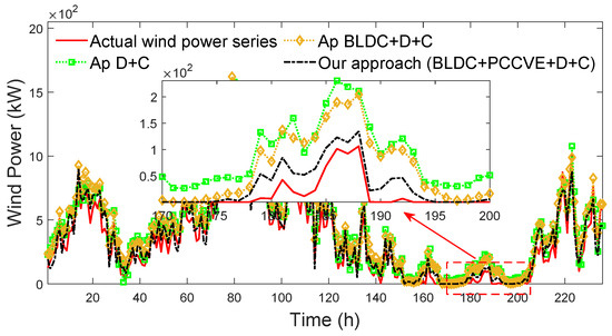
Figure 19.
Forecasted wind power series of different approaches (forecast horizon h = 1).
In Figure 19, viewing from the distance of each approach from the forecasted wind power series to the actual wind power series, it can be seen that the distance of Ap D+C is largest, the distance of Ap BLDC+D+C is moderate, and the distance of our approach is smallest, especially between time 170 and time 200. The forecasting errors and runtimes of different approaches are shown in Table 5.
Table 5.
Forecasting errors and runtimes of different approaches.
In Table 5, it can be clearly seen that both BLDC and PCCVE effectively reduce forecasting error but also increase runtime. Viewing the forecasting error of Ap D+C and Ap BLDC+D+C, it can be seen that BLDC reduces NRMSE by 0.51% and NMAE by 0.34%. Viewing the forecasting error of Ap BLDC+D+C and our approach, it can be seen that PCCVE reduces NRMSE by 1.91% and NMAE by 1.85%. Compared with BLDC, PCCVE reduces more forecasting error. Viewing the runtime of these approaches, it can be seen that the runtimes of Ap BLDC+D+C and Ap D+C are close, while the runtime of our approach is nearly six times the runtime of Ap BLDC+D+C. Compared with BLDC, PCCVE increases more runtime. Obviously, PCCVE provides the main contribution to the accuracy and complexity of our approach.
4.5. Performance Comparison of Different Approaches
To comprehensively demonstrate the performance of our approach, the accuracy and complexity of our approach are compared with that of benchmark approaches. Generally, the forecasting approach has three main components: (a) data preprocessing, (b) model forecasting, and (c) model configuration optimization. The greater the difference between different forecasting approaches in three main components, the lower the comparability between them. To ensure the comparability between benchmark approaches and our approach, recent advanced approaches Ap [38], Ap [39], and Ap [40] that have similar main components to our approach are selected as benchmark approaches. The detailed implementations of benchmark approaches and our approach are shown in Table 6.
Table 6.
Detailed implementations of benchmark approaches and our approach.
In Table 6, it can be seen that Ap [38], Ap [39], Ap [40], and our approach all use box-plot in data preprocessing to deal with outlier wind speed points, all select the deep neural network in model forecasting to forecast wind power, and all use the heuristic optimization in model configuration optimization to optimize the values of main hyperparameters. The number of main hyperparameters of Ap [38], Ap [39], Ap [40], and our approach is 17, 9, 6, and 12, respectively. Compared with Ap [38], Ap [39], and Ap [40], the number of main hyperparameters of our approach is moderate. To further ensure the fairness of the comparison, during the implementation of Ap [38], Ap [39], Ap [40], and our approach, the common main hyperparameters that need to be optimized are set to belong to the same value ranges. Specifically, = , = , = , and = . The common main hyperparameters that need to be given directly are set to the same value. Specifically, PS = 20 and MG = 100. The remaining main hyperparameters of these approaches are set through the trial–error method. In addition, the persistence model, as the popular and simple forecasting approach, is often used to demonstrate the performance of other approaches. Therefore, the persistence model is also used as a benchmark approach in the comparison. The forecasted wind power series of different approaches under forecast horizon h = 1 are shown in Figure 20.
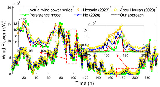
Figure 20.
Forecasted wind power series of different approaches (forecast horizon h = 1) [38,39,40].
In Figure 20, it can be clearly seen that in most situations, actual wind power moderately fluctuates, and the forecasted wind power series of all approaches well approximate the actual wind power series. Furthermore, in some situations, actual wind power severely fluctuates, and the forecasted wind power series of our approach better approximate the actual wind power series than that of other approaches, especially between time 90 and time 105. The reason is that PCCVE adapts to the non-stationarity degree of historical wind speed series and more accurately gives the estimated error of CNN-BiLSTM-MHA, which guides the optimization algorithm to better configure the values of CNN-BiLSTM-MHA’s hyperparameters. It ensures CNN-BiLSTM-MHA more effectively constructs the complex wind speed–power mapping relationship to better forecast the wind power under severe wind power fluctuations. However, in few situations, actual wind power has no fluctuation and remains around 0, and the forecasted wind power series of the persistence model better approximates the actual wind power series than that of our approach, especially between time 170 and time 200. This is because in these few situations, the fluctuation of actual wind power does not follow the fluctuation of actual wind speed, which makes it difficult for our approach, as well as Ap [38], Ap [39], and Ap [40] to effectively construct the wind speed–power mapping relationship to forecast the wind power. The forecasting way of the persistence model is to keep actual wind power at the last time as forecasted wind power at the next time, which shows its superiority in these few situations. The forecasting errors and runtimes of different approaches under forecast horizon h = 1 are shown in Table 7.
Table 7.
Forecasting errors and runtimes of different approaches (forecast horizon h = 1).
In Table 7, it can be seen that NRMSE and NMAE of our approach are smaller than those of other approaches. In addition, the runtime of our approach is moderate compared with that of other approaches. Specifically, due to our approach and Ap [38] adopting PCCVE and CVE, respectively, the runtimes of our approach and Ap [38] are significantly greater than that of Ap [39] and Ap [40]. Because our approach trains one CNN-LSTM-MHA, while Ap [38] trains multiple LSTMs, the runtime of our approach is lower than that of Ap [38].
Besides, the values of main hyperparameters of Ap [38], Ap [39], Ap [40], and our approach under forecast horizon h = 1 are detailed in Appendix A.
To better demonstrate the adaptability of our approach, the accuracy of different approaches under different forecast horizons are compared. The forecasted wind power series of different approaches under forecast horizon h = 3 are shown in Figure 21.
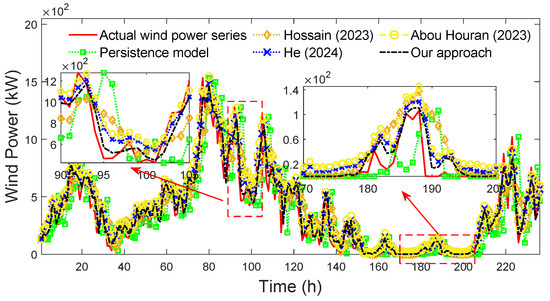
Figure 21.
Forecasted wind power series of different approaches (forecast horizon h = 3) [38,39,40].
The forecasting errors of different approaches under forecast horizon h = 3 are shown in Table 8.
Table 8.
Forecasting errors of different approaches (forecast horizon h = 3).
The forecasted wind power series of different approaches under forecast horizon h = 5 are shown in Figure 22.
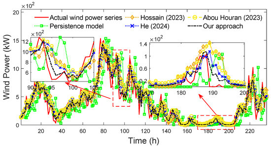
Figure 22.
Forecasted wind power series of different approaches (forecast horizon h = 5) [38,39,40].
The forecasting errors of different approaches under forecast horizon h = 5 are calculated and shown in Table 9.
Table 9.
Forecasting errors of different approaches (forecast horizon h = 5).
By comparing Figure 20, Figure 21 and Figure 22, it can be seen that the performance of all approaches decreases with the increase in forecast horizon, without exception. However, under different forecasting horizons, the forecasted wind speed series of our approach all better approximate the actual wind speed series than that of other approaches, and the forecasting errors of our approach are all smaller, which proves the availability of our approach under different forecasting horizons.
By comprehensively comparing different approaches, it is found that our approach can more accurately forecast wind power with only moderate runtime.
5. Conclusions
In this paper, an approach based on model optimal configuration via prequential-cross cooperative validation estimation is proposed for short-term wind power forecasting.
The main contributions are as follows: (i) to enable CNN-BiLSTM-MHA to efficiently construct the wind speed–power mapping relationship, the prequential-cross cooperative validation estimation based on PVE and CVE is proposed to accurately give the co-estimated error of CNN-BiLSTM-MHA and better assist the optimization of the values of CNN-BiLSTM-MHA’s hyperparameters; (ii) to prevent CNN-BiLSTM-MHA from being interfered by local outlier wind speed points, the box-plot local detection–correction combining the spatial–temporal optimal-weighted fuzzy clustering and the sliding window connected box-plot is proposed for the first time to reasonably detect and correct local outlier wind speed points; and (iii) to ensure the accuracy of the sliding window connected box-plot, the spatial–temporal optimal-weighted fuzzy clustering, which adopts the traditional similarity objective function, novel balance objective function, and non-dominated sorting, is proposed for the first time to effectively mine and provide similar wind speed segments as the detection contexts of multiple sliding window connected box-plots. Furthermore, sufficient experiments demonstrated that our approach accurately and stably forecasts wind power, which is beneficial to the power dispatch of power systems.
The main limitations are as follows: (i) prequential-cross cooperative validation estimation and box-plot local detection–correction are relatively time-consuming; and (ii) prequential-cross cooperative validation estimation is specially designed for forecasting time series tasks, and it is difficult to be extended to other types of tasks. Therefore, how to reduce the time consumption of prequential-cross cooperative validation estimation and box-plot local detection–correction and expand the former to other types of tasks has become the focus of our future research.
Author Contributions
Conceptualization, L.J. and G.W.; methodology, L.J. and G.W.; software, L.J.; validation, G.W. and X.P.; formal analysis, L.J. and X.P.; investigation, G.W.; resources, G.W.; data curation, X.P.; writing—original draft preparation, L.J.; writing—review and editing, G.W.; visualization, L.J.; supervision, G.W.; project administration, G.W.; funding acquisition, G.W. All authors have read and agreed to the published version of the manuscript.
Funding
This work was supported by Fundamental Research Funds for the Central Universities in China (N25ZLE008) and National Natural Science Foundation of China (62373085).
Institutional Review Board Statement
Not applicable.
Informed Consent Statement
Not applicable.
Data Availability Statement
Data in this study are available on request from the corresponding author.
Conflicts of Interest
The authors declare no conflicts of interest.
Appendix A
The main hyperparameters of benchmark approaches and our approach include K (the number of clusters), HN (the number of hidden neurons), IL (the initial learn rates), FS (the number of filters), CK (the size of convolution kernel), DF (the dilation factor), AH (the number of attention heads), KC (the number of key and query channels), PS (the population size), MG (the maximum generations), MR (the migration ratio), MP (the migration period), LD (the ratio of leaders to population), CC (the curve control value), IW (the inertia weight), and N (the number of subsets).
The values of 17 main hyperparameters of Ap [38] are shown in Table A1.
Table A1.
Values of 17 main hyperparameters of Ap [38].
Table A1.
Values of 17 main hyperparameters of Ap [38].
| Main Component | Main Hyperparameter |
|---|---|
| 1st LSTM | HN = 16 and IL = 0.035 |
| 2nd LSTM | HN = 16 and IL = 0.05 |
| 3rd LSTM | HN = 32 and IL = 0.05 |
| 4th LSTM | HN = 32 and IL = 0.05 |
| 5th LSTM | HN = 32 and IL = 0.065 |
| 6th LSTM | HN = 48 and IL = 0.065 |
| Monarch butterfly optimization | PS = 20, MG = 100, MR = 0.4, and MP = 1.2 |
| CVE | N = 10 |
HN and IL are set by the optimization. PS and MG are uniformly set. MR and MP are set by the trial–error method. N is set according to [38].
The values of 9 main hyperparameters of Ap [39] are shown in Table A2.
Table A2.
Values of 9 main hyperparameters of Ap [39].
Table A2.
Values of 9 main hyperparameters of Ap [39].
| Main Component | Main Hyperparameter |
|---|---|
| TCN-LSTM-SA | FS = 32, CK = 3, DF = 2, HN = 48, and IL = 0.05 |
| Improved coot optimization | PS = 20, MG = 100, LD = 0.2, and CC = 5 |
FS, CK, DF, HN, and IL are set by the optimization. PS and MG are uniformly set. LD and CC are set by the trial–error method.
The values of 6 main hyperparameters of Ap [40] are shown in Table A3.
Table A3.
Values of 6 main hyperparameters of Ap [40].
Table A3.
Values of 6 main hyperparameters of Ap [40].
| Main Component | Main Hyperparameter |
|---|---|
| CNN-LSTM | FS = 32, CK = 3, HN = 32, and IL = 0.065 |
| Coati optimization | PS = 20 and MG = 100 |
FS, CK, HN, and IL are set by the optimization. PS and MG are uniformly set.
The values of 12 main hyperparameters of our approach are shown in Table A4.
Table A4.
Values of 12 main hyperparameters of our approach.
Table A4.
Values of 12 main hyperparameters of our approach.
| Main Component | Main Hyperparameter |
|---|---|
| BLDC | K = 4 and D = 2 |
| CNN-BiLSTM-MHA | FS = 32, CK = 3, HN = 48, IL = 0.05, AH = 2, and KC = 2 |
| Dual fitness particle swarm optimization | PS = 20, MG = 100, and IW = 0.9 |
| PCCVE | N = 5 |
K is set according to [33]. D is set by the sobol method [41]. FS, CK, HN, IL, AH, and KC are set by the optimization. PS and MG are uniformly set. IW is set by the trial–error method. N is set by the artificial experience.
References
- Kanagarathinam, K.; Aruna, S.K.; Ravivarman, S.; Safran, M.; Alfarhood, S.; Alrajhi, W. Enhancing sustainable urban energy management through short-term wind power forecasting using lstm neural network. Sustainability 2023, 15, 13424. [Google Scholar] [CrossRef]
- Guo, Z.; Wei, F.; Qi, W.; Han, Q.; Liu, H.; Feng, X.; Zhang, M. A time series prediction model for wind power based on the empirical mode decomposition–convolutional neural network–three-dimensional gated neural network. Sustainability 2024, 16, 3474. [Google Scholar] [CrossRef]
- World Wind Energy Association. WWEA Annual Report 2024: A Challenging Year for Windpower. Available online: https://wwindea.org/GlobalStatistics (accessed on 23 April 2025).
- Mao, J.; Zhao, J.; Zhang, H.; Gu, B. A Novel Hybrid Deep Learning Model for Day-Ahead Wind Power Interval Forecasting. Sustainability 2025, 17, 3239. [Google Scholar] [CrossRef]
- Song, Y.; Tang, D.; Yu, J.; Yu, Z.; Li, X. Short-term forecasting based on graph convolution networks and multiresolution convolution neural networks for wind power. IEEE Trans. Ind. Inform. 2023, 19, 1691–1702. [Google Scholar] [CrossRef]
- Wang, H.; Xue, W.; Liu, Y.; Peng, J.; Jiang, H. Probabilistic wind power forecasting based on spiking neural network. Energy 2020, 196, 117072. [Google Scholar] [CrossRef]
- Pan, C.; Wen, S.; Zhu, M.; Ye, H.; Ma, J.; Jiang, S. Hedge backpropagation based online LSTM architecture for ultra-short-term wind power forecasting. IEEE Trans. Power Syst. 2024, 39, 4179–4192. [Google Scholar] [CrossRef]
- Jonkers, J.; Avendano, D.N.; Van Wallendael, G.; Van Hoecke, S. A novel day-ahead regional and probabilistic wind power forecasting framework using deep CNNs and conformalized regression forests. Appl. Energy 2024, 361, 122900. [Google Scholar] [CrossRef]
- Al-Yahyai, S.; Charabi, Y.; Gastli, A. Review of the use of numerical weather prediction (NWP) models for wind energy assessment. Renew. Sust. Energ. Rev. 2010, 14, 3192–3198. [Google Scholar] [CrossRef]
- Zhang, J.; Yan, J.; Infield, D.; Liu, Y.; Lien, F.S. Short-term forecasting and uncertainty analysis of wind turbine power based on long short-term memory network and Gaussian mixture model. Appl. Energy 2019, 241, 229–244. [Google Scholar] [CrossRef]
- Bikcora, C.; Verheijen, L.; Weiland, S. Density forecasting of daily electricity demand with ARMA-GARCH, CAViaR, and CARE econometric models. Sustain. Energy Grids Netw. 2018, 13, 148–156. [Google Scholar] [CrossRef]
- Yunus, K.; Thiringer, T.; Chen, P. ARIMA-based frequency-decomposed modeling of wind speed time series. IEEE Trans. Power Syst. 2016, 31, 2546–2556. [Google Scholar] [CrossRef]
- Wang, Y.; Zou, R.; Liu, F.; Zhang, L.; Liu, Q. A review of wind speed and wind power forecasting with deep neural networks. Appl. Energy 2021, 304, 117766. [Google Scholar] [CrossRef]
- Shams, M.H.; Niaz, H.; Hashemi, B.; Liu, J.J.; Siano, P.; Anvari-Moghaddam, A. Artificial intelligence-based prediction and analysis of the oversupply of wind and solar energy in power systems. Energy Conv. Manag. 2021, 250, 114892. [Google Scholar] [CrossRef]
- Wolpert, D.H.; Macready, W.G. An efficient method to estimate bagging’s generalization error. Mach. Learn. 1999, 35, 41–55. [Google Scholar] [CrossRef]
- Wang, X.; Luo, D.; Zhao, X.; Sun, Z. Estimates of energy consumption in China using a self-adaptive multi-verse optimizer-based support vector machine with rolling cross-validation. Energy 2018, 152, 539–548. [Google Scholar] [CrossRef]
- Wu, Z.; Xia, X.; Xiao, L.; Liu, Y. Combined model with secondary decomposition-model selection and sample selection for multi-step wind power forecasting. Energy 2020, 261, 114345. [Google Scholar] [CrossRef]
- Lainder, A.D.; Wolfinger, R.D. Forecasting with gradient boosted trees: Augmentation, tuning, and cross-validation strategies: Winning solution to the M5 Uncertainty competition. Int. J. Forecast. 2022, 38, 1426–1433. [Google Scholar] [CrossRef]
- Krawczuk, J.; Łukaszuk, T. The feature selection bias problem in relation to high-dimensional gene data. Artif. Intell. Med. 2016, 66, 63–71. [Google Scholar] [CrossRef] [PubMed]
- Cerqueira, V.; Torgo, L.; Mozetič, I. Evaluating time series forecasting models: An empirical study on performance estimation methods. Mach. Learn. 2020, 109, 1997–2028. [Google Scholar] [CrossRef]
- Bergmeir, C.; Hyndman, R.J.; Koo, B. A note on the validity of cross-validation for evaluating autoregressive time series prediction. Comput. Stat. Data Anal. 2018, 120, 70–83. [Google Scholar] [CrossRef]
- Bergmeir, C.; Benítez, J.M. On the use of cross-validation for time series predictor evaluation. Inf. Sci. 2012, 191, 192–213. [Google Scholar] [CrossRef]
- Wang, G.; Jia, R.; Liu, J.; Zhang, H. A hybrid wind power forecasting approach based on Bayesian model averaging and ensemble learning. Renew. Energy 2020, 145, 2426–2434. [Google Scholar] [CrossRef]
- McGill, R.; Tukey, J.W.; Larsen, W.A. Variations of box plots. Am. Stat. 1978, 33, 12–16. [Google Scholar] [CrossRef]
- Smiti, A. A critical overview of outlier detection methods. Comput. Sci. Rev. 2020, 38, 100306. [Google Scholar] [CrossRef]
- Liu, S.; Liu, X.; Lyu, Q.; Li, F. Comprehensive system based on a DNN and LSTM for predicting sinter composition. Appl. Soft Comput. 2020, 95, 106574. [Google Scholar] [CrossRef]
- Fang, P.; Fu, W.; Wang, K.; Xiong, D.; Zhang, K. A compositive architecture coupling outlier correction, EWT, nonlinear Volterra multi-model fusion with multi-objective optimization for short-term wind speed forecasting. Appl. Energy 2022, 307, 118–191. [Google Scholar] [CrossRef]
- Blázquez-García, A.; Conde, A.; Mori, U.; Lozano, J.A. A review on outlier/anomaly detection in time series data. ACM Comput. Surv. 2022, 54, 1–33. [Google Scholar] [CrossRef]
- Angiulli, F.; Fassetti, F. Distance-based outlier queries in data streams: The novel task and algorithms. Data Min. Knowl. Discov. 2010, 20, 290–324. [Google Scholar] [CrossRef]
- Deb, K.; Pratap, A.; Agarwal, S.; Meyarivan, T.A.M.T. A fast and elitist multiobjective genetic algorithm: NSGA-II. IEEE Trans. Evol. Comput. 2002, 6, 182–197. [Google Scholar] [CrossRef]
- Li, Z.; Li, L.; Chen, J.; Wang, D. A multi-head attention mechanism aided hybrid network for identifying batteries’ state of charge. Energy 2024, 286, 129504. [Google Scholar] [CrossRef]
- Rezaei, F.; Safavi, H.R. Sustainable conjunctive water use modeling using dual fitness particle swarm optimization algorithm. Water Resour. Manag. 2022, 36, 989–1006. [Google Scholar] [CrossRef]
- Wang, G.; Jia, L.; Xiao, Q. A hybrid approach based on unequal span segmentation-clustering for short-term wind power forecasting. IEEE Trans. Power Syst. 2023, 39, 203–216. [Google Scholar] [CrossRef]
- Sun, G.; Jiang, C.; Cheng, P.; Liu, Y.; Wang, X.; Fu, Y.; He, Y. Short-term wind power forecasts by a synthetical similar time series data mining method. Renew. Energy 2018, 115, 575–584. [Google Scholar] [CrossRef]
- Xia, J.; Shang, P.; Wang, J.; Shi, W. Permutation and weighted-permutation entropy analysis for the complexity of nonlinear time series. Commun. Nonlinear Sci. Numer. Simul. 2016, 31, 60–68. [Google Scholar] [CrossRef]
- DiCiccio, T.J.; Efron, B. Bootstrap confidence intervals. Stat. Sci. 1996, 11, 189–228. [Google Scholar] [CrossRef]
- Hintze, J.L.; Nelson, R.D. Violin plots: A box plot-density trace synergism. Am. Stat. 1998, 52, 181–184. [Google Scholar] [CrossRef]
- Hossain, M.A.; Gray, E.; Lu, J.; Islam, M.R.; Alam, M.S.; Chakrabortty, R.; Pota, H.R. Optimized forecasting model to improve the accuracy of very short-term wind power prediction. IEEE Trans. Ind. Inform. 2023, 19, 10145–10159. [Google Scholar] [CrossRef]
- He, X.; He, B.; Qin, T.; Lin, C.; Yang, J. Ultra-short-term wind power forecasting based on a dual-channel deep learning model with improved coot optimization algorithm. Energy 2024, 305, 132320. [Google Scholar] [CrossRef]
- Abou Houran, M.; Bukhari, S.M.S.; Zafar, M.H.; Mansoor, M.; Chen, W. COA-CNN-LSTM: Coati optimization algorithm-based hybrid deep learning model for PV/wind power forecasting in smart grid applications. Appl. Energy 2023, 349, 121638. [Google Scholar] [CrossRef]
- Lai, X.; Meng, Z.; Wang, S.; Han, X.; Zhou, L.; Sun, T.; Li, X.; Wang, X.; Ma, Y.; Zheng, Y. Global parametric sensitivity analysis of equivalent circuit model based on Sobol’method for lithium-ion batteries in electric vehicles. J. Clean. Prod. 2021, 294, 126246. [Google Scholar] [CrossRef]
Disclaimer/Publisher’s Note: The statements, opinions and data contained in all publications are solely those of the individual author(s) and contributor(s) and not of MDPI and/or the editor(s). MDPI and/or the editor(s) disclaim responsibility for any injury to people or property resulting from any ideas, methods, instructions or products referred to in the content. |
© 2025 by the authors. Licensee MDPI, Basel, Switzerland. This article is an open access article distributed under the terms and conditions of the Creative Commons Attribution (CC BY) license (https://creativecommons.org/licenses/by/4.0/).