Article

Study on RSEI Changes Using Remote Sensing and Markov-FLUS Modeling Approach

1
Hainan Academy of Ocean and Fisheries Sciences, Haikou 572000, China
2
Yazhou Bay Innovation Institute, Hainan Tropical Ocean University, Sanya 570100, China
3
Hainan Aerospace Technology Innovation Center, Wenchang 571333, China
4
School of Geography and Environmental Sciences, Hainan Normal University, Haikou 571158, China
*
Author to whom correspondence should be addressed.
Sustainability 2025, 17(22), 10267; https://doi.org/10.3390/su172210267
Submission received: 1 October 2025 / Revised: 6 November 2025 / Accepted: 10 November 2025 / Published: 17 November 2025
(This article belongs to the Special Issue Environmental Planning and Governance for Sustainable Cities)

Abstract

With the rapid advancement of the Hainan Free Trade Port (HFTP), substantial changes in land use and ecological systems have emerged. The study analyzes the spatiotemporal dynamics of ecological quality in Hainan Province from 2017 to 2024 and projects its potential evolution through 2030 under different development scenarios. A comprehensive framework integrating the Remote Sensing Ecological Index (RSEI) and Land Use/Cover Change (LUCC) simulations was employed. Multi-source datasets, including remote sensing imagery, geographic, meteorological, and socio-economic data, were combined with the Markov–FLUS model to simulate future land-use patterns. The results indicate extensive urban expansion and a notable increase in construction land, accompanied by a continuous decline in RSEI values, particularly under the business-as-usual scenario. In contrast, policy-guided simulations suggest more sustainable land allocation and gradual improvement in ecological quality. The findings demonstrate that integrating scenario-based simulation with ecological index modeling provides an effective approach for supporting ecological conservation and sustainable urban planning in tropical island regions experiencing rapid economic transformation.

1. Introduction

Land use and land cover (LULC) serves as a key indicator of the complex interactions between human activities and the natural environment [1]. It not only reflects the pace of urbanization but also mirrors the spatial heterogeneity of ecological quality. Rapid urban expansion accelerates land-use transitions, increases the intensity of human activities, and triggers ecological issues such as biodiversity loss, soil erosion, and deforestation [2]. Therefore, exploring Land Use/Cover Change (LUCC) dynamics is essential for understanding the mechanisms linking urban growth, ecological degradation, and sustainable regional development. As urban construction land expands, the structure and function of ecosystems are profoundly altered, highlighting the need for rapid, quantitative, and spatially explicit methods to assess ecological quality across multiple scales.
Ecological environment quality refers to the extent to which ecological factors within a specific space and time support human survival and sustainable socio-economic development [3]. Early evaluations mainly relied on qualitative or semi-quantitative methods such as the Analytic Hierarchy Process (AHP) [4], expert scoring [5], and grey correlation analysis [6]. Although these methods provided valuable initial insights, their subjectivity and limited spatial visualization constrained both accuracy and scalability. With the advancement of remote sensing technology, ecological assessment has evolved toward data-driven and quantitative frameworks capable of monitoring long-term environmental changes. In the early stages, single indicators such as the Normalized Difference Vegetation Index (NDVI) [7] and Land Surface Temperature (LST) [8] were used as proxies for ecosystem health. However, single-variable approaches failed to capture the multi-dimensional nature of ecological processes. To overcome these limitations, Xu (2013) [9] introduced the RSEI, which integrates four key components: greenness, humidity, heat, and dryness, using principal component analysis. The RSEI has proven effective in producing objective and comprehensive assessments of ecological conditions and has been widely applied to evaluate ecosystem health across different regions and time periods.
Land use evolution is driven by the combined effects of natural conditions, socio-economic development, and policy interventions. Recent research has investigated LUCC mechanisms from various perspectives, including human–land system coupling [10], impacts on ecosystem services [11], and the spatial drivers of land transitions [12]. However, most research has focused on ecologically fragile or environmentally stressed areas such as arid and mountainous regions [13,14], while the complex feedbacks between LUCC and ecological quality under intensive, policy-driven economic transformation remain underexplored. Accurate simulation and prediction of LUCC are essential for promoting sustainable land resource utilization and effective environmental management. Various models, including System Dynamics [15], CLUE-S [16], SLEUTH [17], Cellular Automata [18], and Markov models [19], have been extensively used, yet their ability to capture spatial heterogeneity and nonlinear conversion dynamics varies. The Markov–FLUS model, which combines transition probability with a self-adaptive cellular automata framework, has shown superior performance in reproducing realistic spatial dynamics of land-type transformations [20,21].
In recent years, Hainan Province has become a national testing ground for China’s new stage of institutional openness and sustainable development. The Hainan Free Trade Port (HFTP), officially launched in 2020 as the first and only free trade port covering an entire island province, is guided by the Master Plan for the Construction of the HFTP [22]. The initiative aims to build a globally competitive, innovation-driven, and low-tariff economy by 2035 through liberalized trade and investment mechanisms. Within the broader framework of China’s ecological civilization policy, the HFTP serves as a strategic experiment in balancing rapid economic liberalization with ecological sustainability [22].
The implementation of these transformative policies has profoundly reshaped Hainan’s spatial development patterns. Rapid expansion of urban construction land, industrial parks, transport infrastructure, and tourism facilities has intensified pressure on limited land resources and fragile island ecosystems [23]. Experiences from other free trade zones such as Hong Kong, Singapore, and Dubai suggest that liberalized trade and investment can promote technological diffusion, industrial upgrading, and more efficient land use [24,25], yet may also generate negative externalities, including pollution displacement and ecological degradation under weak environmental governance [26,27]. In tropical island ecosystems with limited environmental carrying capacities, such risks can quickly lead to irreversible ecological damage.
Despite increasing policy interest, most current research on the HFTP remains focused on its economic performance, trade facilitation, and institutional innovation [28]. Spatially explicit and quantitative analyses integrating LUCC dynamics with ecological quality indicators remain limited. The lack of such studies restricts a comprehensive understanding of how HFTP-related policies influence land-use transitions and ecological resilience. Examining the impacts of policy-driven development under the HFTP on regional land-use structure, ecosystem function, and overall ecological quality is therefore of both scientific and practical significance.
To address this gap, the present study integrates multi-temporal remote sensing data, the RSEI, and the Markov–FLUS simulation framework to analyze the spatiotemporal impacts of HFTP development on land use and ecological environment quality in Hainan Province. By analyzing LUCC patterns from 2017 to 2024 and projecting future land-use scenarios through 2030, the study provides empirical evidence on how large-scale policy interventions and economic transformation reshape the ecological landscape of a tropical island. The findings contribute to the broader discussion on sustainable urbanization and policy evaluation, offering insights to support decision-making that balances economic growth with environmental protection in rapidly developing free trade ports.
The structure of the paper is as follows. Section 2 describes the study area and data sources. Section 3 presents the methodology, including LULC classification, land use intensity index, RSEI construction, and the Markov–FLUS model. Section 4 reports the main results on land-use change, ecological environment quality, and simulation outcomes. Section 5 discusses the findings in the context of existing research, and Section 6 concludes the study and outlines future research directions.

2. Study Area and Materials

2.1. Study Area

Haikou City (19°31′32″–20°04′52″ N, 110°07′22″–110°42′32″ E) is located in the northern part of Hainan Province and characterized by a tropical marine monsoon climate. The terrain is predominantly flat with gentle undulations, consisting mainly of plains and terraced farmlands interspersed with rivers and wetlands. Haikou administers four districts: Xiuying, Longhua, Qiongshan, and Meilan. Serving as the political, economic, technological, cultural, and transportation center of Hainan Province, the city holds a pivotal position in regional development [29]. The spatial distribution of the study area is presented in Figure 1.

2.2. Datasets and Materials

The research utilized remote sensing imagery along with key geographic, meteorological, and socio-economic datasets. The remote sensing data included Sentinel-2 land-use data for Haikou City from 2017 to 2024, Landsat 8 OLI/TIRS images from 2017 and 2024, and Sentinel-2A images for the same years. The geographic data comprised the vector boundary of Haikou City and digital elevation model (DEM) data. Meteorological variables included annual mean temperature (TEM), total annual rainfall (RAI), and mean annual wind speed (WIN). Socio-economic data covered population (POP), gross domestic product (GDP), railway length (LRRL), highway length (LRDL), and information obtained from the Haikou Statistical Yearbooks. A summary of all datasets is provided in Table 1.
The land cover data used in this study were obtained from the Sentinel-2 Land Cover Explorer, which provides global land-use information at a 10 m spatial resolution for the period 2017–2024. The dataset, developed by Impact Observatory, Microsoft, and Esri through a deep-learning–based land classification model, employs the UTM (WGS84) coordinate system. Based on the research objectives, land-use types were reclassified into seven categories: Water, Trees, Flooded Vegetation, Crops, Built Area, Range Land, and Others (including Bare Ground and Clouds).
To ensure the accuracy of surface reflectance data and minimize the effects of atmospheric interference, cloud cover, and shadow contamination, Landsat 8 Surface Reflectance (SR) imagery was preprocessed using a cloud and shadow masking algorithm within the Google Earth Engine (GEE) platform (https://code.earthengine.google.com). The procedure followed the standard preprocessing steps recommended by the United States Geological Survey (USGS) for Landsat Collection 2 Level-2 products.
The quality assurance band (QA_PIXEL) was used to identify and remove pixels affected by clouds and cloud shadows. Bitwise operations were applied to decode the relevant bits representing clouds (bit 4) and cloud shadows (bit 3). Pixels meeting either condition were excluded by assigning a mask value of zero, while clear-sky pixels were retained. The masking operation was defined as Equation (1):
m a s k   =   ( Q A   _   P I X E L   &   2 3   =   0 )     ( Q A _   P I X E L   &   2 4   =   0 )  
The resulting mask was applied to the surface reflectance bands to generate a cloud-free composite. All reflectance values were then scaled by a factor of 0.0001 (i.e., divided by 10,000) to convert digital numbers (DNs) to surface reflectance values ranging from 0 to 1. Temporal metadata were preserved to maintain the integrity of the time-series dataset.

3. Methodology

The methodological framework of this study is illustrated in Figure 2, which integrates multi-source data, land use simulation models, and ecological evaluation techniques to analyze the spatiotemporal changes in ecological status in HFTP from 2017 to 2024.
First, multi-source datasets were collected as inputs, including remote sensing images (2017–2024), DEM and MODIS data, and meteorological and socio-economic datasets. The methodological workflow comprised six key modules: (1) LULC Classification: The standard land cover dataset provided by Esri and Impact Observatory was reclassified into seven categories according to the actual conditions of the study area: Water, Trees, Flooded Vegetation, Crops, Built Area, Range Land, and Others (including Bare Ground and Clouds); (2) Ecological Factor Extraction: Ecological indicators including NDVI, Land Surface Temperature (LST), Normalized Difference Built-up and Soil Index (NDBSI), and Tasseled Cap Wetness (TCP) were extracted from Landsat and DEM data to form the basis for RSEI; (3) Driving Factor Identification: Socio-economic and policy-related variables were used to identify the main driving forces influencing land-use changes, including infrastructure expansion and policy planning; (4) Land Use Simulation: The Markov–FLUS model was employed to simulate future land-use scenarios. A Markov transition probability matrix was calculated to estimate future land demand, while the future land use simulation (FLUS)model generated spatially explicit land-use patterns for 2030; (5) Ecological Quality Assessment: Principal Component Analysis (PCA) was used to integrate multiple ecological indicators into a unified RSEI. Both current and simulated LUCC data were incorporated into the spatiotemporal RSEI framework to detect ecological trends under different development scenarios; (6) Ecological Trend Evaluation: The final module synthesized all results to assess ecological change trends and provide insights for sustainable land management and environmental policy formulation within the HFTP.

3.1. LULC Classification and Change Dynamics

The land use transition matrix [30] provides a quantitative depiction of land structure and its temporal transformations across different periods. This method is useful for understanding the dynamics of LULC changes. Formula (2) presents the mathematical representation of the land-use transition matrix. Data covering eight periods from 2017 to 2024 were generated and analyzed to examine patterns and trends of land-use transformations in Haikou City.
S i j = S 11 S 12 S 1 n S 21 S 22 S 2 n S n 1 S n 2 S n n
S i j represents the area of land category i that has been transformed into category j , while n denotes the total number of land-use classes.

3.2. Comprehensive Index of Land Use Intensity

The degree of land use quantifies the extent and intensity of land utilization, reflecting the combined influence of human activities and natural environmental conditions [31]. Following the comprehensive land use degree assessment framework proposed by Zhuang et al. [31], land use is classified into four categories according to the equilibrium state of the natural land complex. Table 2 provides the detailed classification of the indices. The land use degree index model is given [32] by Formula (3):
L j = 100 × i = 1 n A i × C i
L j represents the land use degree index, while A i denotes the grading index corresponding to the i -level of land use degree. The variable C i indicates the area percentage for land use level i , while n specifies the number of land use categories. The land use degree index varies between 100 and 400, with higher values indicating greater intensity of land utilization.

3.3. Construction of Remote Sensing Ecological Index

The RSEI was applied to evaluate the ecological status of the study area, following the method proposed by [9]. The index integrates four core indicators: (1) NDVI, which represents vegetation greenness derived from the red and near-infrared (NIR) bands; (2) LST, derived from Landsat thermal infrared bands or MODIS products; (3) NDBSI, which quantifies surface dryness by combining the Index-based Built-up Index (IBI) and the Soil Index (SI); (4) WET, which indicates surface moisture extracted through Tasseled Cap transformation. The RSEI provides an integrated assessment of ecosystem health by leveraging remote sensing and geographic information systems (GISs), demonstrating the advantages of interdisciplinary environmental monitoring [33].
In this study, the GEE platform was used to process Landsat 8 and Sentinel-2 imagery for the target year (January–December). Cloud filtering was conducted to retain images with the lowest cloud coverage, and time-series interpolation was applied to fill missing values. Four ecological component indicators directly related to urban environmental quality: greenness (NDVI), wetness (TCW), dryness (NDBSI), and heat (LST). The component indicators and their respective formulas are presented in Table 3 [34].
During the data processing stage, NDVI, WET, and NDBSI were derived from Sentinel-2 MSI surface reflectance products with a spatial resolution of 10 m, while LST was calculated from Landsat 8 TIRS thermal bands (30 m resolution) using the single-channel algorithm. All input indicators were normalized to a range of 0–1 prior to PCA to ensure comparability.
To minimize the influence of subjective judgment in assigning weights, the selected indicators (NDVI, WET, NDBSI, LST) were combined using PCA [35]. The first principal component (PC1) was used to construct the RSEI, as it captures the majority of the variance among the indicators. Since each indicator has different units and numerical scales, normalization was performed to standardize all variables within the 0–1 range [36]. To ensure that higher PC1 values correspond to better ecological conditions, eigenvalue analysis was conducted on the GEE platform. The initial RSEI (RSEI0) was obtained by subtracting PC1 from 1, as shown in Equation (4). Finally, RSEI0 was standardized to generate the final RSEI (Equation (5)), enabling consistent comparison across temporal and spatial scales.
I ( N I ) = I I m i n I m a x I m i n
where I ( N I ) represents the normalized pixel value of a certain indicator factor, I represents the pixel value of a specific indicator factor, and I m a x and I m i n represent the maximum and minimum values of that indicator factor (Equation (5)).
R S E I 0 = 1 P C 1 f N D V I , W E T , N D S B I , L S T
All indicators were normalized to a 0–1 range before performing PCA. The PC1, which accounted for more than 85% of the total variance, was extracted as the RSEI. A higher RSEI value indicates a better ecological condition, as shown in Equation (6).
R S E I = R S E I 0 R S E I 0   m i n R S E I 0   m a x R S E I 0   m i n
where RSEI values range from 0 to 1, with higher values indicating better ecological conditions, and vice versa for poorer ecological environment quality. R S E I 0 m a x and R S E I 0 m i n represent the maximum and minimum values of the R S E I 0 index, respectively.
To determine the relative contribution of each indicator objectively, PCA was applied to the four normalized indices. PCA transforms the original correlated variables into orthogonal components that maximize the total variance explained. The PC1, which accounted for more than 85% of the total variance across all study years, was extracted as the synthetic ecological component. The factor loadings of PC1 represent the relative contribution (weight) of each ecological indicator to overall ecological quality. In all years, NDVI and WET exhibited positive loadings, whereas LST and NDBSI showed negative loadings, consistent with ecological theory indicating that higher vegetation greenness and surface moisture correspond to better environmental conditions, while dryness and heat are associated with ecological degradation.
Accordingly, the RSEI was constructed from PC1 and linearly scaled to a range of 0–1 (Equation (7)):
R S E I = f P C 1 =   P C 1 P C 1 m i n   P C 1 m a x     P C 1 m i n  
Higher RSEI values indicate better ecological quality. This approach ensures that the ecological index is data-driven, objective, and reproducible, thereby avoiding the subjectivity inherent in weight assignment methods such as expert scoring or the AHP. The PCA-based weighting framework follows the methodology established and has been validated in subsequent ecological remote sensing studies [9,37,38].
To ensure the reliability and comparability of the RSEI across years, a temporal consistency analysis of the PCA loadings was conducted for the period 2017–2024. The results showed that the PC1 consistently explained more than 80 percent of the total variance, confirming its dominant role in representing overall ecological quality. The loadings of the four indicators, namely NDVI (greenness), WET (humidity), LST (heat), and NDBSI (dryness), remained stable throughout the study period. NDVI and WET displayed strong positive correlations with PC1, whereas LST and NDBSI showed strong negative correlations. The stable pattern indicates that PC1 effectively captures the ecological gradient from favorable green and moist conditions to degraded hot and dry environments.
Interannual variations in loading coefficients were minimal, with differences below 5 percent for all indicators, indicating strong temporal robustness of the PCA fusion process. The stable signs and relative magnitudes of the loadings further confirm the comparability of RSEI values across different years. This stability suggests that variations in RSEI primarily reflect genuine ecological changes rather than statistical inconsistencies in PCA weighting.
In addition, the consistent directionality of the indicators ensures that RSEI values retain a uniform ecological interpretation over time, with higher values consistently representing better ecological quality. The complete PCA loading matrices for all study years are presented in Table 4, and the PCA variance ratios are shown in Table 5 to ensure reproducibility and transparency. These results verify the methodological validity of using PC1 as the foundation of the RSEI and confirm the temporal reliability of the ecological assessment framework adopted in this study.

3.4. Markov-Plus Module and Driving Factors

Land-use change is influenced by the combined effects of multiple factors, and the dominant drivers vary across regions and time periods. The selection of appropriate driving factors is essential for developing reliable land-use prediction models and simulating future spatial patterns. Considering the natural geographical characteristics, socio-economic development conditions, data availability, scientific validity, and sustainability of the study area, eight driving factors were selected based on previous studies on land-use change mechanisms [39,40,41]. These driving factors encompass four aspects: topographic conditions, socio-economic factors, climate factors, and transportation location. To ensure consistency, all datasets were standardized with unified coordinate systems, identical row and column numbers, and consistent spatial resolution. Each dataset was converted into TIF format to complete the parameter set used for land-use prediction in Haikou City.
To ensure the robustness of the land-use simulation, eight driving factors were selected, namely population density, GDP density, distance to roads, distance to coastline, elevation, slope, NDVI, and land-use intensity. These factors were identified based on their established influence on land-use dynamics and ecological processes in coastal regions [42,43].
To quantitatively assess their suitability, a Pearson correlation analysis was conducted between each driving factor and the observed land-use transitions from 2010 to 2020. The results showed that all variables exhibited significant correlations with land-use change at the 95 percent confidence level (p < 0.05). GDP density and population density demonstrated strong positive correlations (r = 0.63 and 0.59, respectively), indicating that socio-economic drivers play a leading role in urban expansion. NDVI and slope were negatively correlated with the growth in construction land (r = 0.42 and 0.37, respectively), suggesting that ecological and topographic constraints continue to influence spatial development in Hainan.
For model transparency, spatial distribution maps of all driving factors were generated, and descriptive statistics, including mean, standard deviation, and range, were summarized. These results confirm the spatial heterogeneity and rational selection of the driving factors incorporated into the model.
In this research, a combined Markov–FLUS model was utilized to dynamically simulate and forecast LUCC in Haikou. Within the FLUS framework, the Cellular Automata (CA) module, which incorporates an adaptive inertia mechanism, manages spatial distribution by simulating interactions among neighboring cells [44]. The Markov model complements this process by estimating the magnitude of changes across different land-use categories.
(1)
Markov Model and Transition Probability Matrix Construction
To simulate future changes in ecological quality, this study integrated the Markov chain model with the FLUS framework, enabling spatially explicit prediction of RSEI dynamics driven by land-use transitions. The integrated Markov–FLUS model combines the probabilistic land-use conversion mechanism of the Markov chain with the spatial allocation capability of the FLUS module, allowing the simultaneous representation of temporal transition probabilities and spatial heterogeneity.
The Markov model estimates the probability of conversion between different land-use categories based on observed transitions during two historical periods. The transition probability matrix P i j was computed as (Equation (8)):
P i j = N i j j = 1 K N i j
where K is the number of land-use categories. Each row of the matrix P = P i j sums to one and describes the probability that a pixel of class i will become class j in the next time step.
The land-use area vector at time t + δ t is then projected by Equation (9):
A t + δ t = A t × P
Multi-step projections (e.g., to 2030) are obtained by repeated multiplication P n . The resulting projected land-use area demands serve as non-spatial constraints within the FLUS model, which spatially allocates land-use transitions based on suitability maps, neighborhood interactions, and inertia coefficients. Through this integrated framework, the Markov process quantifies the magnitude of land-use change, whereas the FLUS model determines its spatial distribution.
(2)
FLUS Model Parameterization
The FLUS model applies an adaptive Cellular Automata (CA) mechanism that incorporates both driving factors and neighborhood effects to simulate land-use dynamics. The neighborhood influence was parameterized using a 5 × 5 Moore neighborhood, in which the transition probability of each central cell is affected by the composition of its surrounding cells according to a weighted neighborhood function (Equation (10)):
Ω k x , y , t = m , n N W k δ k   m , n , t  
where Ω k x , y , t represents the neighborhood influence of land-use type t at location ( x , y ) , W k is the neighborhood weight, and δ k ( m , n , t ) indicates the presence of type k in the neighborhood.
The inertia coefficient α k was introduced to represent the resistance of each land-use category to change, providing a balance between stability and transition potential. Typical values ranged from 0.2 to 0.8, depending on the historical stability of each category. Urban and built-up areas were assigned higher inertia coefficients to reflect strong planning and regulatory constraints, whereas cropland and forest areas were given lower values, indicating greater flexibility for land-use conversion.
(3)
Driving Factors and Model Calibration
Eight spatial driving factors were selected as explanatory variables: elevation, slope, distance to roads, distance to rivers, distance to built-up areas, population density, GDP density, and policy zoning related to the HFTP development area. All factors were normalized and incorporated as input layers into the FLUS suitability module based on transition rules derived from logistic regression.
Model calibration was performed by comparing the simulated 2022 land-use map with the actual 2022 land-use data using the Kappa coefficient and the Figure of Merit (FoM). The optimal parameter combination yielded a Kappa value of 0.64 and an overall accuracy (OA) of 0.75, demonstrating a high level of simulation reliability.
(4)
Coupling with RSEI Evaluation
The simulated land-use maps for 2030 under different policy scenarios (business-as-usual, eco-protection, and HFTP-accelerated) were then used to compute RSEI distributions. For each scenario, the RSEI was reconstructed by integrating four indicators: NDVI, WET, LST, and NDBSI, which were derived from Landsat and Sentinel imagery. The PCA-based RSEI calculation was applied consistently across all time periods to ensure comparability. The resulting RSEI maps represent predicted ecological quality outcomes influenced by land-use transitions simulated through the Markov and FLUS models.
The coupled model simulated the spatial distribution of land use in 2030 through three main steps. First, 2018 was selected as the base year, and driving factor parameters were input into the ANN module of the GeoSOS FLUS platform to generate a probability map of land-use suitability. Based on this, land-use data for 2022 were simulated. Second, the Validation module compared the simulated and actual land-use data for 2022. The Kappa coefficient, OA, and FoM were used to evaluate the accuracy and reliability of the Markov FLUS model. Third, using the 2022 land-use data as the starting point, rivers and reservoirs were incorporated as constraint layers for future land-use change, and the CA module was then applied to predict the spatial distribution of land use in 2030. Among them, the accuracy evaluation index FOM (Figure of Merit) [45] is a statistical index that can directly measure the accuracy of the predicted changes, representing the consistency between the actual and simulated results. Its formula can be expressed as Equation (11):
F O M = B / ( A + B + C + D )
Here, A denotes the number of pixels that actually changed, but were incorrectly predicted as unchanged; B indicates the number of correctly predicted pixels where both actual and simulated changes occurred; C refers to the number of pixels that underwent actual change and were predicted to change, but to a different land-use category; D refers to pixels where no real change occurred, yet the model predicted a change. The FoM index ranges from 0 to 1, with higher values indicating better model performance.

4. Results

4.1. Spatiotemporal Dynamics of Land Use in Haikou City

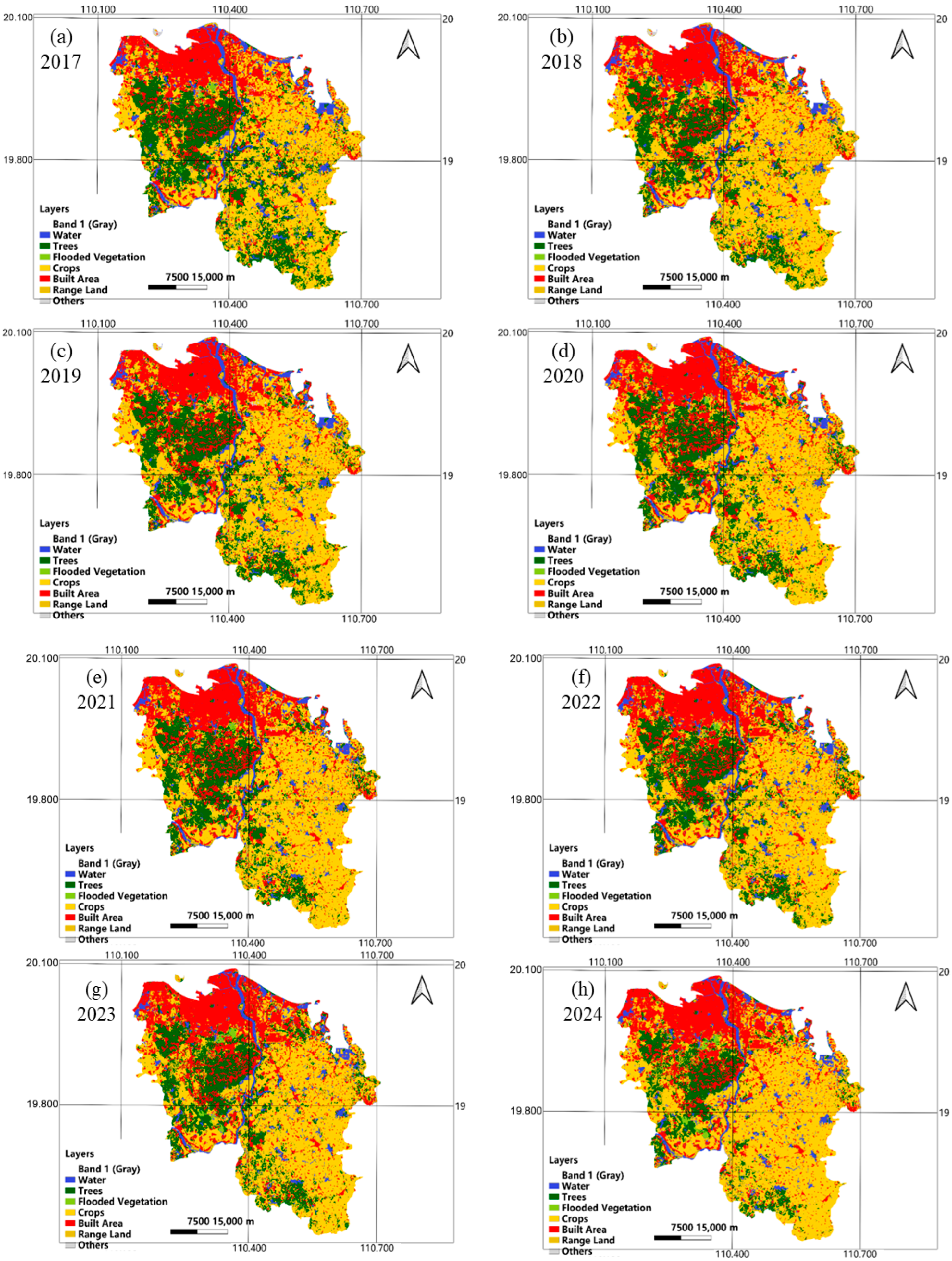
Subplots (a) to (f) Figure 3 presents the land-use and land-cover distribution in Haikou City from 2017 to 2024, and Table 6 summarizes the quantitative changes across land-use categories. Distinct regional differences in land-use patterns were observed during the study period. The southern part of Haikou City, which remains less economically developed, is dominated by agricultural landscapes consisting mainly of cropland and forested areas. The construction of the HFTP resulted in a noticeable increase in built-up areas, which became more spatially concentrated and expanded by less than 100 km2 over eight years. The main driving force behind these changes was large-scale deforestation associated with infrastructure construction, a pattern similar to that observed in other rapidly developing regions of China. The expansion of construction land was accompanied by a decline in cropland and a reduction in water bodies and areas classified as “Others,” while rangeland and flooded vegetation showed a modest increase. These changes suggest that a substantial portion of ecological space was converted for production and development purposes, posing considerable challenges to the ecological environment of Haikou City.

4.2. Land Use Transition Matrix

During the study period, land-use changes in Haikou City were mainly characterized by conversions among built-up areas, cropland, forest, and rangeland, as shown in Table 7. The expansion of built-up land was largely driven by the conversion of cropland, while the increase in cropland mainly resulted from the transformation of forested areas. The reduction in forest cover was primarily attributed to its conversion into cropland. The HFTP construction plan requires significant land for urban infrastructure, residential areas, and industrial parks. Trees and crops are considered viable land resources. To accommodate rapid urban growth, arable land was occupied and forested areas were cleared. As a result, forest land decreased by 247.17 km2, cropland increased by 133.32 km2, built-up land expanded by 71.93 km2, and rangeland increased by 52.59 km2. Ecological protection measures, including large-scale vegetation restoration, led to the conversion of flooded vegetation mainly into cropland and forested areas. The area categorized as “Others” showed a minor outflow of only 2.005 km2, primarily converted into built-up land and grassland for construction and ecological restoration purposes.

4.3. Land Use Intensity Comprehensive Index

The comprehensive land use intensity index reflects the degree of land utilization within the study area. The calculated values for Haikou City from 2017 to 2024 are illustrated in Figure 4. The most significant increase occurred between 2017 and 2018. Despite various challenges, Haikou City maintained steady progress, and the implementation of major urban projects such as the Meilan Airport Phase II and highway expansion contributed to this rise in land use intensity. A slight decline in the index was observed between 2018 and 2023, which may be attributed to the city’s adherence to the new development philosophy and the continued regulation of urban and rural construction land under the Hainan Free Trade Zone policy. These measures helped guide urban expansion in a more controlled and sustainable manner. From 2023 to 2024, the index increased sharply. Considering the strategic context of this period, the change reflects the combined effects of multiple national and provincial initiatives. The accelerated development of the HFTP was the main factor driving the rapid growth in land use intensity.
The period from 2023 to 2024 represents a crucial stage in preparing for the island’s closed-border operations. As the provincial capital and the economic and cultural center of Hainan, Haikou has undertaken the construction of numerous core facilities. The expansion and intelligent upgrading of Meilan Airport, the New Seaport, and Macun Port, together with the construction of second-tier ports such as the New Seaport Passenger Transport Hub, have required substantial land resources. To implement the policy of “opening first-tier ports and controlling second-tier ports,” large areas have been designated for bonded warehouses, inspection sites, and processing zones, all of which exhibit high land-use intensity. To support the Free Trade Port’s development, Haikou City has initiated a series of key infrastructure projects outlined in the Fourteenth Five-Year Plan. The Haikou Jiangdong New District, as a core pilot zone of the Free Trade Port, entered a phase of rapid development and investment promotion during 2023 and 2024. The construction of industrial parks and facilities for the headquarters economy, airport-related industries, and modern service sectors progressed intensively, resulting in extensive land leveling and development activities. Consequently, land-use intensity in and around the district increased sharply. To attract and retain talent for the Free Trade Port, Haikou City also accelerated the construction of talent apartments and affordable housing, which further expanded the scale and intensity of residential land use. The fundamental reason for the marked rise in Haikou’s land-use intensity index between 2023 and 2024 lies in the final preparations for the island-wide closure of the HFTP. To meet the deadline for completing all necessary infrastructure, the city launched numerous large-scale projects, including port facilities, transportation hubs, industrial parks, and support infrastructure. The extensive land requirements and concentrated construction periods of these projects directly contributed to the rapid increase in construction land area and the sharp rise in the land-use intensity index.

4.4. Evaluation of Ecological Environment Quality in Haikou City

4.4.1. Results of the RESI Model

Table 6 presents the PC1 results and average RSEI values for Haikou City from 2017 to 2024. The contribution rate of PC1 exceeded 70 percent in all years, indicating that it effectively captured the main information contained in the ecological indicators. The loadings of NDBSI and LST in PC1 were negative, while those of NDVI and WET were positive. These findings suggest that dryness and heat exerted negative effects on the ecological environment of Haikou City, whereas vegetation greenness and surface moisture had positive influences. The observed relationships are consistent with the overall ecological development trends. Based on these results, the PC1 components of the four indicators were integrated to construct the RSEI model, which was applied to evaluate the ecological environment quality of Haikou City.

4.4.2. Dynamic Changes in Ecological Environment Status

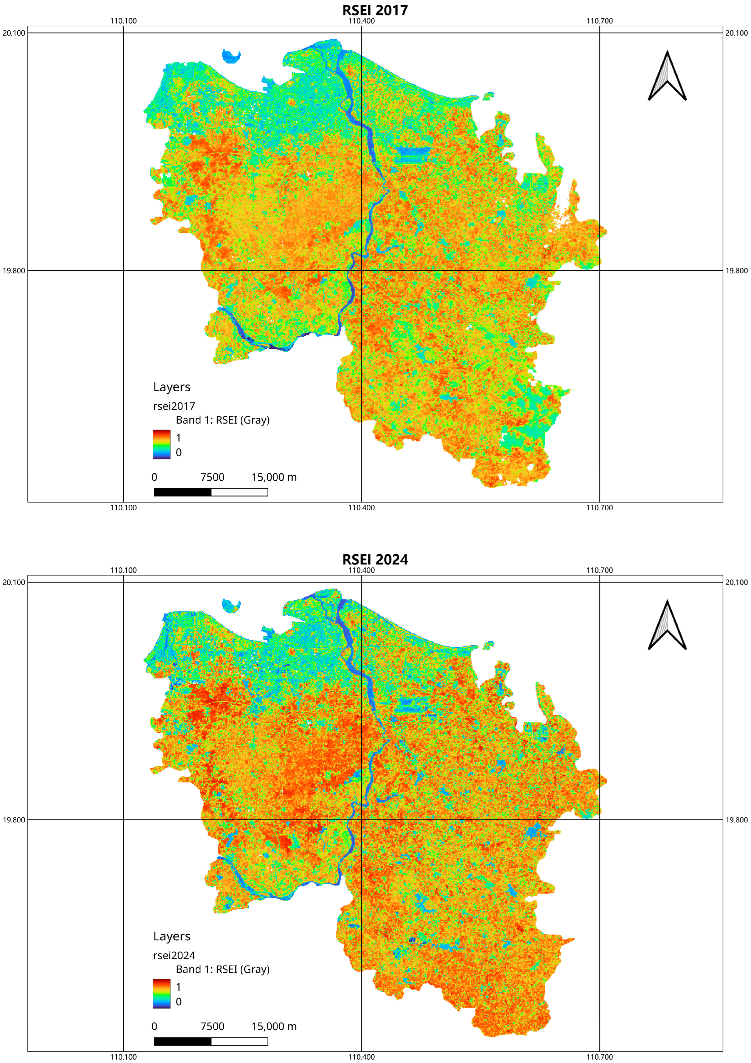
Figure 5 illustrates the spatial distribution of RSEI values in Haikou City, revealing pronounced spatial differences in ecological environment quality. Areas with lower ecological quality are mainly concentrated in the northern urban sectors and along water bodies, where human activity is most intensive. In contrast, regions with higher ecological quality are located primarily in the southern areas, which are characterized by dense vegetation cover and limited urban development. Noticeable improvements in ecological conditions occurred in forest parks, woodlands, grasslands, and wetland parks, whereas areas with lower ecological quality were mainly associated with barren land and newly developed construction zones. These patterns indicate that ecological development initiatives under the HFTP framework have contributed to environmental enhancement in Haikou City.
Although regional ecological restoration efforts in areas such as the West Coast, Haikou Bay, and Dongzhai Port have yielded positive outcomes, rapid urbanization has led to an overall decline in ecological quality. The average RSEI value decreased from 0.730 in 2017 to 0.649 in 2024, reflecting a general downward trend. This reduction highlights a gap between the current ecological condition and the high environmental standards targeted by the Free Trade Port. Figure 6 presents the statistical classification of RSEI values. The excellent and good grades together accounted for more than 65 percent of the total area, suggesting that Haikou’s overall ecological environment remains at a relatively high level. In 2017, the proportion of areas classified as excellent (Grade 5) was the highest, while in 2022, the majority shifted to the good category (Grade 4). This shift indicates that large-scale construction projects, including Meilan International Airport Phase II and the Ring Road Phase II, reduced vegetation coverage in newly developed areas, thereby lowering ecological quality.
To evaluate the statistical significance of changes in ecological quality, the Mann–Kendall trend test and paired t-tests were applied to annual RSEI values from 2017 to 2024. Spatial autocorrelation was examined using Global Moran’s I and Local Getis–Ord Gi indices based on a Queen contiguity matrix. A significantly positive Moran’s I value (p < 0.01) indicated clear spatial clustering of low RSEI values in key development zones, while the Gi analysis revealed ecological hot spots and cold spots that corresponded to areas experiencing intense urbanization.

4.5. Land Use Simulation Results

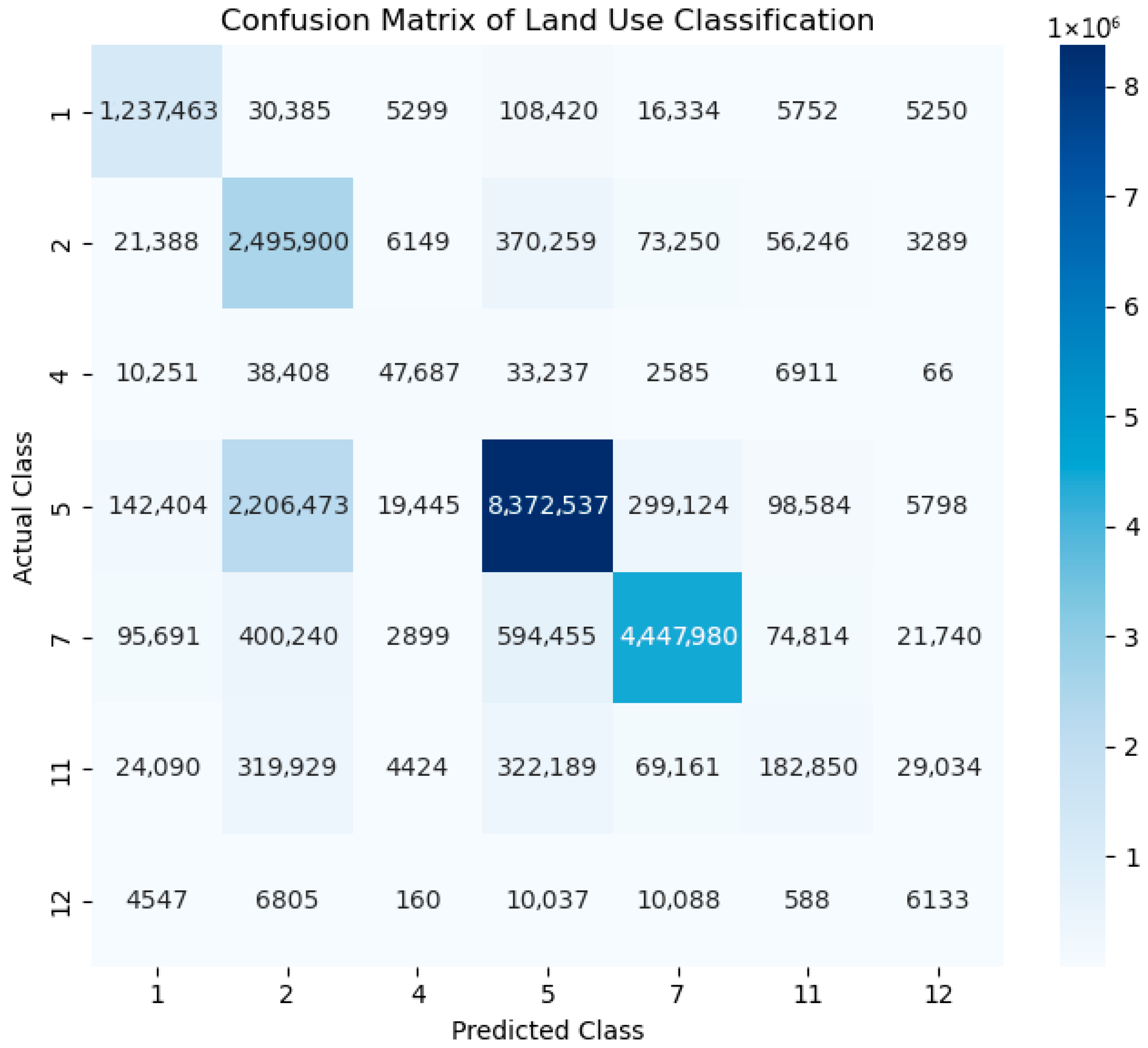
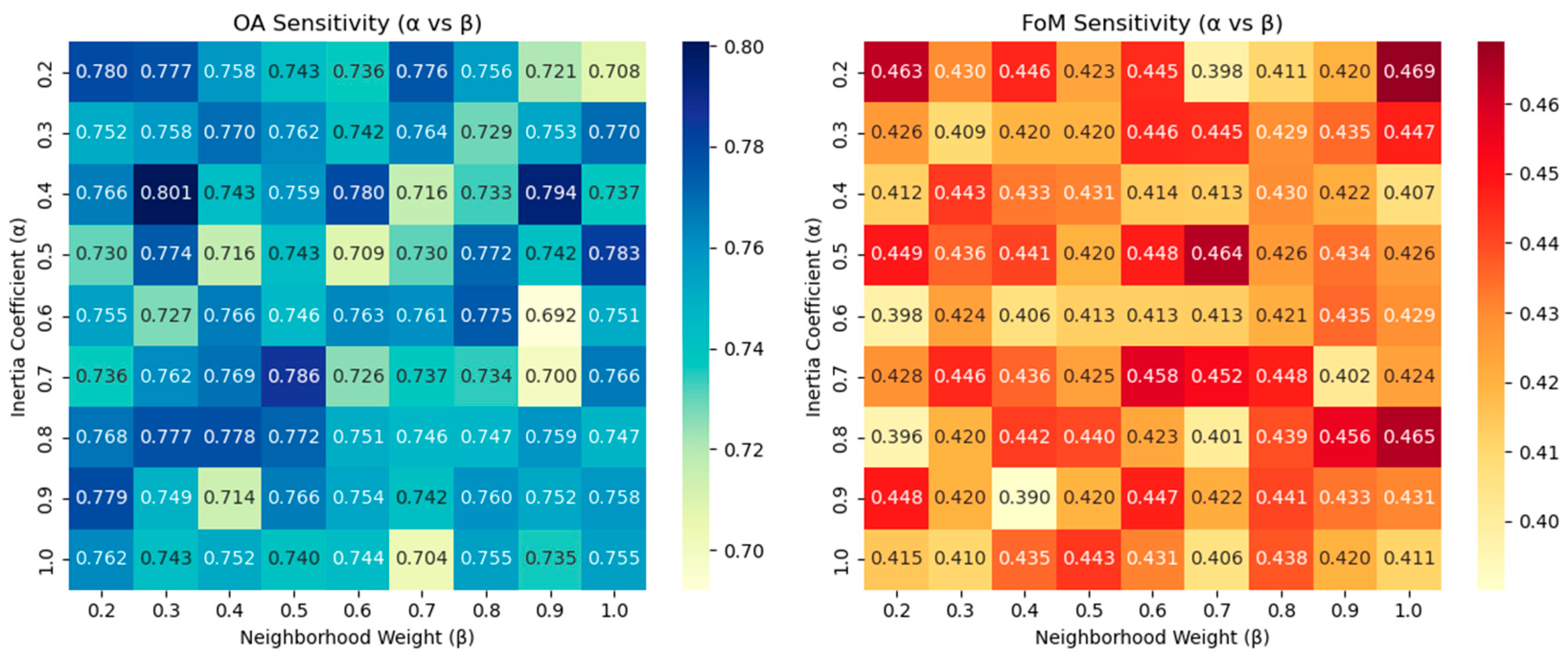
A probability map was generated based on the selected driving factors by incorporating the 2018 land-use data into the CA module of the Markov–FLUS model. The simulated land-use map for 2022 was then produced and compared with the actual 2022 land-use data to evaluate model accuracy. The model parameters were configured with 300 iterations, a neighborhood size of 3, and a model acceleration factor of 0.1. The simulated land quantities were adjusted to match the actual 2022 land-use distribution. The confusion matrix (Figure 7), sensitivity analysis of the FLUS model parameters (Figure 8), and accuracy assessment yielded an OA of 0.75, a Kappa coefficient of 0.63, and a k value of 0.741, indicating strong spatial consistency between simulated and observed results. These outcomes confirm that the model can reliably simulate future land-use dynamics in the study area.
User’s Accuracy (UA) and Producer’s Accuracy (PA) were calculated for each land-use category based on the confusion matrix comparing the simulated 2022 map with the actual 2022 land-use classification. The validation of the Markov–FLUS simulation results was further enhanced through three steps.
(1)
A complete confusion matrix was added to present the classification performance of each land-use category.
(2)
Class-wise UA and PA values were provided to evaluate the spatial prediction reliability of each category, as shown in Table 8.
(3)
A sensitivity analysis was conducted on key FLUS model parameters, including the inertia coefficient and neighborhood weights, to assess their effects on simulation accuracy.
Based on the 2022 land-use data and the development probabilities of different land-use categories, the projected spatial distribution of land use in 2030 is shown in Figure 6. The central urban area of Haikou is expected to experience limited change and remain largely saturated, while surrounding towns are anticipated to undergo considerable expansion as built-up land extends outward from the city core. The northeastern part of Haikou is projected to become increasingly dominated by construction land. In the future, cropland is expected to continue declining, while built-up areas will expand substantially, reflecting a sustained upward trend in urbanization. Statistical projections of land-use areas for 2030 are summarized in Table 9. The cropland area is predicted to decrease significantly from 1009.625 km2 in 2022 to 878.772 km2 in 2030 (shown as Figure 9). In contrast, built-up land is expected to show the largest proportional increase among all categories. This expansion is likely driven by continuous improvements in infrastructure planning and talent introduction policies under the HFTP initiative. As urbanization accelerates and the population continues to grow, the demand for built-up land will rise, leading to extensive conversion of cropland into urban construction areas.

5. Analysis and Discussion

5.1. Analysis of Land Use Changes in Haikou City

This study evaluated the spatiotemporal change characteristics of LUCC in Haikou City from 2017 to 2024. The results indicated that cropland, built-up areas, and forest consistently occupied the largest proportions of land use. An overall increase in built-up land and a decline in forest area were observed, which aligns with previous research findings. Lin X et al. [29] analyzed the spatiotemporal evolution of cultivated land in Haikou City from 1980 to 2020 and reported a continuous decline in cultivated land after 2010, consistent with the observed reduction in cropland between 2018 and 2020 in this study. The decline in agricultural land can be attributed mainly to urban expansion, which has encroached on large areas of farmland. Numerous studies [46,47,48] have shown that regional economic development directly affects land use change. According to data from the Haikou Municipal Bureau of Statistics, Haikou has prioritized high-quality economic development in recent years, significantly strengthening its economic capacity. The city’s GDP grew by an average of 6.5 percent annually, reaching 213.4 billion yuan in 2022, which accounted for 31.3 percent of the provincial total. During this period, built-up land in Haikou increased markedly. The continuous development of road networks and municipal infrastructure projects in the Jiangdong New Area improved connectivity among urban clusters, enhanced public facilities, and promoted industrial expansion. These developments reinforced the ecological foundation and shaped the city’s spatial structure. The significant increase in construction land in the Jiangdong New Area observed in this study corresponds well with actual development patterns.

5.2. Discussion of Changes in RSEI in Haikou

Our research results indicate that from 2017 to 2024, the proportion of RSEI values in the “good” and “excellent” ranges for Haikou City exceeded 65%, reflecting a generally favorable ecological environment consistent with actual conditions [49]. However, rapid economic growth and urban expansion have led to a continuous increase in impervious surfaces, which have replaced ecological land, reduced vegetation coverage, and created challenges for management authorities in enforcing control measures within protected areas. These changes have significantly affected the overall quality of the regional ecological environment. Areas with low RSEI values are mainly concentrated in regions with intensive human activity, such as Longhua District, Meilan District, and the northern part of Xiuying District. In contrast, higher RSEI values are primarily distributed across the southern parts of Longhua and Qiongshan Districts. This spatial pattern indicates that accelerated urbanization contributes to environmental degradation, consistent with the findings of Hussain M. [50]. Although the construction of the HFTP has emphasized both economic development and ecological protection, certain projects, including the Nanhai Pearl Artificial Island, have negatively affected coastal wetlands and diminished the ecological quality of nearby areas. In addition, deforestation and illegal mining have caused localized damage to natural resources and the ecological environment. Xin Fang et al. [51] applied the RSEI model to assess the ecological landscape of Hainan Island and concluded that intensified human activities have deteriorated ecological quality, a conclusion consistent with the findings of the present study.

5.3. Comparison with Related Studies

Compared with representative studies conducted in other major coastal regions of China, such as the Guangdong–Hong Kong–Macao Greater Bay Area (GBA) and the Pearl River Delta (PRD), the present study demonstrates both methodological and contextual advancements. Previous research in the GBA and PRD [52,53,54] mainly relied on long-term Landsat series data to construct the RSEI and simulate land-use transitions through CA–Markov, FLUS, or improved models. These studies effectively revealed the influence of rapid urbanization and policy heterogeneity on ecological quality changes, yet most lacked explicit quantitative evaluation of policy-driven scenarios.
At the city scale, research in Singapore and other Southeast Asian cities [55,56] has explored the spatial dynamics of urban green spaces and ecological quality preservation through compact urban planning and greening strategies. Although RSEI or similar indices have been applied in Vietnamese cities such as Can Tho and Ho Chi Minh City [57], most of these analyses remain descriptive and rarely integrate RSEI-based ecological assessment with spatially explicit land-use simulation models such as Markov–FLUS.
In contrast, the present study integrates RSEI-based ecological quality assessment with the Markov–FLUS simulation framework to quantitatively establish the linkage among driving factors, land-use transition, and ecological response. The HFTP policy scenario is explicitly incorporated as a modeling variable, enabling the projection and comparison of spatial impacts under different policy pathways, including business-as-usual and policy-guided scenarios. Incorporating policy scenarios into spatial simulation provides direct evidence for evaluating the ecological consequences of large-scale development initiatives, an aspect that has been largely neglected in previous research.
Moreover, this research extends the application of RSEI and FLUS modeling into a tropical island context, where coastal ecosystems are more sensitive to land-use pressures and climate variability than in mainland regions. Through detailed model calibration, sensitivity analysis, and spatially explicit validation, the study enhances both methodological transparency and policy relevance in remote-sensing-based ecological evaluation. The proposed framework offers a replicable and policy-responsive approach for supporting sustainable land-use planning in island-based free trade ports and tropical coastal regions worldwide.

6. Conclusions

Under the context of the HFTP construction, the study integrates multi-source remote sensing data, RSEI modeling, and the Markov–FLUS simulation framework to analyze land-use changes and ecological environment quality in Haikou City. The results show that urban construction land expanded rapidly under HFTP-driven urbanization, particularly in key development areas such as Jiangdong New Area, leading to a marked decline in cultivated land and a reorganization of the city’s spatial structure. The RSEI analysis indicates that the overall ecological environment quality remains moderate, with pronounced spatial heterogeneity. Higher ecological quality is observed in the northern coastal zones and central ecological corridors, while lower RSEI values occur in central urban areas and regions near ports where anthropogenic pressure is intense.
Based on the Markov–FLUS projections for 2030, priority areas for ecological conservation were identified, including mangrove belts along the northern coast and central ecological corridors. These zones require strict protection and active ecological restoration. Urban expansion should be directed toward existing urban cores to reduce encroachment on high-quality ecological areas. Recommended land-use regulation strategies include restricting built-up land expansion in low-RSEI regions, restoring degraded agricultural lands, and promoting compact urban development to enhance land-use efficiency while minimizing ecological disturbance.
Furthermore, balancing economic development with ecological conservation during HFTP construction requires policy integration and green governance. Incentives for industrial upgrading, green infrastructure, and ecological compensation mechanisms should be applied in newly developed areas. Scenario-based simulations from the Markov–FLUS model can provide spatial guidance for optimizing land allocation, thereby supporting sustainable development and long-term ecological security in Haikou City.

Author Contributions

P.L.: Conceptualization, Data curation, Visualization, Writing—original draft. T.W.: Investigation, Validation. S.W.: Software, Investigation, Methodology. R.H.: Funding acquisition, Investigation, Writing—review and editing. All authors have read and agreed to the published version of the manuscript.

Funding

This work was supported by Hainan Provincial Natural Science Foundation of China (Grant Number 624QN255); the Major Science and Technology Plan Project of Yazhou Bay Innovation Research Institute of Hainan Tropical Ocean College (2022CXYZD003).

Institutional Review Board Statement

Not applicable.

Informed Consent Statement

Not applicable.

Data Availability Statement

The data presented in this study are available on request from the corresponding author.

Acknowledgments

The authors would like to thank the anonymous reviewers and editor for constructive comments and suggestions.

Conflicts of Interest

The authors declare that they have no known competing financial interests or personal relationships that could have appeared to influence the work report in this paper.

References

  1. Wang, Q.; Wang, H. Spatiotemporal dynamics and evolution relationships between land-use/land cover change and landscape pattern in response to rapid urban sprawl process: A case study in Wuhan, China. Ecol. Eng. 2022, 182, 106716. [Google Scholar] [CrossRef]
  2. Bajocco, S.; De Angelis, A.; Perini, L.; Ferrare, A.; Salvati, L. The impact of land use/land cover changes on land degradation dynamics: A Mediterranean case study. Environ. Manag. 2012, 49, 980–989. [Google Scholar] [CrossRef]
  3. Zhu, C.; Zhang, X.; Zhou, M.; He, S.; Gan, M.; Yang, L.; Wang, K. Impacts of urbanization and landscape pattern on habitat quality using OLS and GWR models in Hangzhou, China. Ecol. Indic. 2020, 117, 106654. [Google Scholar] [CrossRef]
  4. Zhang, R.; Zhang, X.; Yang, J.; Yuan, H. Wetland ecosystem stability evaluation by using Analytical Hierarchy Process (AHP) approach in Yinchuan Plain, China. Math. Comput. Model. 2013, 57, 366–374. [Google Scholar] [CrossRef]
  5. Wang, Y.; Ding, Q.; Zhuang, D. An eco-city evaluation method based on spatial analysis technology: A case study of Jiangsu Province, China. Ecol. Indic. 2015, 58, 37–46. [Google Scholar] [CrossRef]
  6. Özçelik, F.; Öztürk, B.A. Evaluation of Banks’ Sustainability Performance in Turkey with Grey Relational Analysis. J. Account. Financ. 2014, 63, 189–208. [Google Scholar]
  7. Pettorelli, N.; Vik, J.O.; Mysterud, A.; Gaillard, J.; Tucker, C.; Stenseth, N.C. Using the satellite-derived NDVI to assess ecological responses to environmental change. Trends Ecol. Evol. 2005, 20, 503–510. [Google Scholar] [CrossRef]
  8. Hu, Y.; Xu, E.; Kim, G.; Liu, C.; Tian, G. Response of spatio-temporal differentiation characteristics of habitat quality to land surface temperature in a fast urbanized city. Forests 2021, 12, 1668. [Google Scholar] [CrossRef]
  9. Xu, H.Q. A remote sensing urban ecological index and its application. Acta Ecol. Sin. 2013, 33, 7853–7862. [Google Scholar]
  10. Wu, L.; Yang, Y.; Xie, B. Modeling Analysis on Coupling Mechanisms of Mountain–Basin Human–Land Systems: Take Yuxi City as an Example. Land 2022, 11, 1068. [Google Scholar] [CrossRef]
  11. Cabral, P.; Feger, C.; Levrel, H.; Chambolle, M.; Basque, D. Assessing the impact of land-cover changes on ecosystem services: A first step toward integrative planning in Bordeaux, France. Ecosyst. Serv. 2016, 22, 318–327. [Google Scholar] [CrossRef]
  12. Meneses, B.M.; Reis, E.; Pereira, S.; Maria, J.V.; Reis, R. Understanding driving forces and implications associated with the land use and land cover changes in Portugal. Sustainability 2017, 9, 351. [Google Scholar] [CrossRef]
  13. Fang, Z.; Ding, T.; Chen, J.; Xue, S.; Zhou, Q.; Wang, Y.; Wang, Y.; Huang, Z.; Yang, S. Impacts of land use/land cover changes on ecosystem services in ecologically fragile regions. Sci. Total Environ. 2022, 831, 154967. [Google Scholar] [CrossRef] [PubMed]
  14. Tan, J.; Yu, D.; Li, Q.; Tan, X.; Zhou, W. Spatial relationship between land-use/land-cover change and land surface temperature in the Dongting Lake area, China. Sci. Rep. 2020, 10, 9245. [Google Scholar] [CrossRef]
  15. Zhang, Z.; Li, X.; Liu, X.; Zhao, K. Dynamic simulation and projection of land use change using system dynamics model in the Chinese Tianshan mountainous region, central Asia. Ecol. Model. 2024, 487, 110564. [Google Scholar] [CrossRef]
  16. Waiyasusri, K.; Yumuang, S.; Chotpantarat, S. Monitoring and predicting land use changes in the Huai Thap Salao Watershed area, Uthaithani Province, Thailand, using the CLUE-s model. Environ. Earth Sci. 2016, 75, 533. [Google Scholar] [CrossRef]
  17. Clarke, K.C.; Johnson, J.M. Calibrating SLEUTH with big data: Projecting California’s land use to 2100. Comput. Environ. Urban Syst. 2020, 83, 101525. [Google Scholar] [CrossRef]
  18. Tong, X.; Feng, Y. A review of assessment methods for cellular automata models of land-use change and urban growth. Int. J. Geogr. Inf. Sci. 2020, 34, 866–898. [Google Scholar] [CrossRef]
  19. Islam, M.S.; Ahmed, R. Land use change prediction in Dhaka city using GIS aided Markov chain modeling. J. Life Earth Sci. 2011, 6, 81–89. [Google Scholar] [CrossRef]
  20. Zhu, K.; Cheng, Y.; Zang, W.; Zhou, Q.; Archi, Y.E.; Mousazadeh, H.; Kabil, M.; Csoban, K.; David, L.D. Multiscenario Simulation of Land-Use Change in Hubei Province, China Based on the Markov-FLUS Model. Land 2023, 12, 744. [Google Scholar] [CrossRef]
  21. Chen, Z.; Huang, M.; Zhu, D.; Altan, O. Integrating remote sensing and a markov-FLUS model to simulate future land use changes in Hokkaido, Japan. Remote Sens. 2021, 13, 2621. [Google Scholar] [CrossRef]
  22. Overall Plan for the Construction of Hainan Free Trade Port [EB/OL]. (2020-06-08). Available online: https://www.hnftp.gov.cn/zcfg/zcwj/zyzc/201810/t20181017_3023768.html (accessed on 6 November 2025).
  23. Ma, Y.; Mao, M.; Xie, Z.; Mao, S.; Wang, Y.; Chen, Y.; Xu, J.; Liu, T.; Gong, W.; Wu, L. Spatiotemporal Dynamics and Simulation of Landscape Ecological Risk and Ecological Zoning Under the Construction of Free Trade Pilot Zones: A Case Study of Hainan Island, China. Land 2025, 14, 940. [Google Scholar] [CrossRef]
  24. Chiu, S.W.; Siu, K.Y. Hong Kong as an International Hub: The Rise of Hong Kong in the Modern World-System. In Hong Kong Society: High-Definition Stories Beyond the Spectacle of East-Meets-West; Palgrave Macmillan: Singapore, 2022. [Google Scholar]
  25. Zeng, D.Z. Global Experiences with Special Economic Zones with a Focus on China and Africa. J. Int. Commer. Econ. Policy 2015, 7, 11–20. [Google Scholar]
  26. McAusland, C.; Copeland, B.R.; Taylor, M.S. Trade and Environment: Theory and Evidence; Princeton University Press: Princeton, NY, USA, 2003. [Google Scholar] [CrossRef]
  27. Dean, J.; Lovely, M.; Wang, H. Are foreign investors attracted to weak environmental regulations? Evaluating the evidence from China. Int. Econ. Integr. Domest. Perform 2017, 58, 155–168. [Google Scholar] [CrossRef]
  28. Dong, Q.; Bian, Z. Meeting International Economic and Trade Rules: A Case Study of Hainan Free Trade Port, China. World Cust. J. 2024, 18, 81–99. [Google Scholar] [CrossRef]
  29. Lin, X.; Fu, H. Spatial-Temporal Evolution and Driving Forces of Cultivated Land based on the PLUS Model: A Case Study of Haikou City 1980–2020. Sustainability 2022, 14, 14284. [Google Scholar] [CrossRef]
  30. Munsi, M.; Malaviya, S.; Oinam, G.; Joshi, P.K. A landscape approach for quantifying land-use and land-cover change (1976–2006) in middle Himalaya. Reg. Environ. Change 2010, 10, 145–155. [Google Scholar] [CrossRef]
  31. Zhuang, D.F.; Liu, J.Y. Study on the model of regional differentiation of land use degree in China. J. Nat. Resour. 1997, 12, 105–111. [Google Scholar]
  32. Liu, F.; Yang, G.; Han, X.; Jia, G.; Wang, N. Spatial-temporal Evolution of Land Use and Spatial Autocorrelation Analysis in Horqin Sandy Land—A Case Study of Naiman Banner. J. Northwest For. Univ. 2020, 35, 148–157. [Google Scholar]
  33. Wang, K.; Franklin, S.E.; Guo, X.; Cattet, M. Remote sensing of ecology, biodiversity and conservation: A review from the perspective of remote sensing specialists. Sensors 2010, 10, 9647–9667. [Google Scholar] [CrossRef]
  34. Gou, R.; Zhao, J. Eco-environmental quality monitoring in Beijing, China, using an RSEI-based approach combined with random forest algorithms. IEEE Access 2020, 8, 196657–196666. [Google Scholar] [CrossRef]
  35. Wen, X.; Ming, Y.; Gao, Y.; Hu, X. Dynamic monitoring and analysis of ecological quality of Pingtan comprehensive experimental zone, a new type of sea island city, based on RSEI. Sustainability 2019, 12, 21. [Google Scholar] [CrossRef]
  36. Yang, W.; Zhou, Y.; Li, C. Assessment of Ecological Environment Quality in Rare Earth Mining Areas Based on Improved RSEI. Sustainability 2023, 15, 2964. [Google Scholar] [CrossRef]
  37. Muhammad, K.; Kayoko, Y. Analysis and visualization of spatio-temporal variations of ecological vulnerability in Pakistan using satellite observation datasets. Environ. Sustain. Indic. 2024, 23, 100425. [Google Scholar] [CrossRef]
  38. Li, Y.; Tian, H.; Zhang, J.; Liu, S.; Xie, Z.; Shen, W.; Zheng, Z.; Li, M.; Rong, P.; Qin, Y. Detection of spatiotemporal changes in ecological quality in the Chinese mainland: Trends and attributes. Sci. Total Environ. 2023, 884, 163791. [Google Scholar] [CrossRef]
  39. Li, K.; Feng, M.; Biswas, A.; Su, H.; Niu, Y.; Cao, J. Driving factors and future prediction of land use and cover change based on satellite remote sensing data by the LCM model: A case study from Gansu province, China. Sensors 2020, 20, 2757. [Google Scholar] [CrossRef]
  40. Bagaria, P.; Nandy, S.; Mitra, D.; Sivakumar, K. Monitoring and predicting regional land use and land cover changes in an estuarine landscape of India. Environ. Monit. Assess. 2021, 193, 124. [Google Scholar] [CrossRef]
  41. Rafaai, N.H.; Abdullah, S.A.; Reza, M.I.H. Identifying factors and predicting the future land-use change of protected area in the agricultural landscape of Malaysian peninsula for conservation planning. Remote Sens. Appl. Soc. Environ. 2020, 18, 100298. [Google Scholar] [CrossRef]
  42. Li, C.; Huang, J.; Luo, Y.; Wang, J. Spatial Synergy Between Carbon Storage and Emissions in Coastal China: Insights from PLUS-InVEST and OPGD Models. Remote Sens. 2025, 17, 2859. [Google Scholar] [CrossRef]
  43. Yu, Y.; Liu, D.; Hu, S.; Shi, X.; Tang, J. Spatiotemporal Heterogeneity of Vegetation Cover Dynamics and Its Drivers in Coastal Regions: Evidence from a Typical Coastal Province in China. Remote Sens. 2025, 17, 921. [Google Scholar] [CrossRef]
  44. Kourosh Niya, A.; Huang, J.; Kazemzadeh-Zow, A.; Karimi, H.; Keshtkar, H.; Naimi, B. Comparison of three hybrid models to simulate land use changes: A case study in Qeshm Island, Iran. Environ. Monit. Assess. 2020, 192, 302. [Google Scholar] [CrossRef] [PubMed]
  45. Liu, M.; Chen, H.; Qi, L.; Chen, C. LUCC Simulation Based on RF-CNN-LSTM-CA Model with High-Quality Seed Selection Iterative Algorithm. Appl. Sci. 2023, 13, 3407. [Google Scholar] [CrossRef]
  46. Verburg, P.H.; Soepboer, W.; Veldkamp, A.; Limpiada, R.; Espaldon, V.; Mastura, S. Modeling the spatial dynamics of regional land use: The CLUE-S model. Environ. Manag. 2002, 30, 391–405. [Google Scholar] [CrossRef]
  47. Lambin, E.F.; Turner, B.L.; Geist, H.J.; Agbola, S.B.; Angelsen, A.; Bruce, J.W.; Coomes, O.T.; Dirzo, R.; Fischer, G.; Folke, C. The causes of land-use and land-cover change: Moving beyond the myths. Glob. Environ. Change 2001, 11, 261–269. [Google Scholar] [CrossRef]
  48. Mahtta, R.; Fragkias, M.; Güneralp, B.; Mahendra, A.; Reba, M.; Wentz, E.A.; Seto, K.C. Urban land expansion: The role of population and economic growth for 300+ cities. Npj Urban Sustain. 2022, 2, 5. [Google Scholar] [CrossRef]
  49. Xu, D.; Yang, F.; Yu, L.; Zhou, Y.; Li, H.; Ma, J.; Huang, J.; Wei, J.; Xu, Y.; Zhang, C. Quantization of the coupling mechanism between eco-environmental quality and urbanization from multisource remote sensing data. J. Clean. Prod. 2021, 321, 128948. [Google Scholar] [CrossRef]
  50. Hussain, M.; Abbas, A.; Manzoor, S.; Bilal; Ye, C. Linkage of natural resources, economic policies, urbanization, and the environmental Kuznets curve. Environ. Sci. Pollut. Res. 2023, 30, 1451–1459. [Google Scholar] [CrossRef]
  51. Fang, X.; Gao, S. An empirical study on relationship between island ecological environment and socio-economic development from perspective of environmental Kuznets curve (EKC). Ocean Coast. Manag. 2023, 244, 106819. [Google Scholar] [CrossRef]
  52. Yang, C.; Zhang, C.; Li, Q.; Liu, H.; Gao, W.; Shi, T.; Liu, X.; Wu, G. Rapid urbanization and policy variation greatly drive ecological quality evolution in Guangdong-Hong Kong-Macau Greater Bay Area of China: A remote sensing perspective. Ecol. Indic. 2020, 115, 106373. [Google Scholar] [CrossRef]
  53. Jiao, M.; Hu, M.; Xia, B. Spatiotemporal dynamic simulation of land-use and landscape pattern in the Pearl River Delta, China. Sustain. Cities Soc. 2019, 49, 101581. [Google Scholar] [CrossRef]
  54. Wang, Q.; Liu, D.; Gao, F.; Zheng, X.; Shang, Y. A Partitioned and Heterogeneous Land-Use Simulation Model by Integrating CA and Markov Model. Land 2023, 12, 409. [Google Scholar] [CrossRef]
  55. Masoudi, M.; Tan, P.Y.; Fadaei, M. The effects of land use on spatial pattern of urban green spaces and their cooling ability. Urban Clim. 2021, 35, 100743. [Google Scholar] [CrossRef]
  56. Diep, N.T.H.; Nguyen, N.T.; Hieu, D.C.; Huong, N.T.T.; Trang, D.H. Environmental Quality Monitoring Using Remote Sensing Ecological Index (RSEI) in Can Tho City, Vietnam. IOP Conf. Ser. Earth Environ. Sci. 2024, 1345, 012018. [Google Scholar] [CrossRef]
  57. Hien, N.T. Applying the Improved Remote Sensing Ecological Index (IRSEI) for Urban Ecological Assessment in Ho Chi Minh City, VietNam. Earth Environ. Sci. 2025, 1539. [Google Scholar] [CrossRef]
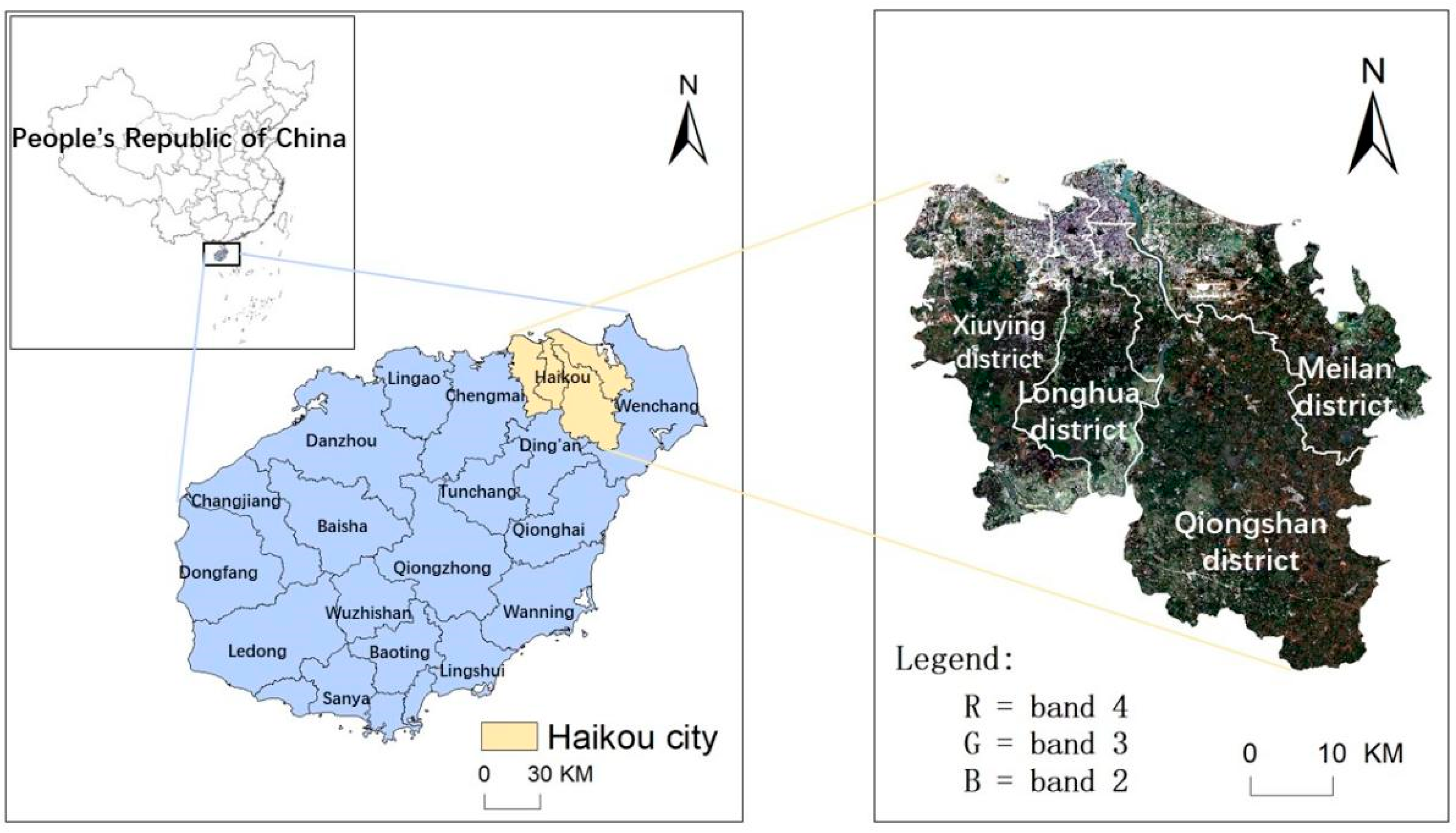
Figure 1. Spatial extent of the study area and remotely sensed data.
Sustainability 17 10267 g001
Figure 2. Flow chart.
Sustainability 17 10267 g002
Figure 3. Land Use Spatial Patterns in Haikou for (a) 2017, (b) 2018, (c) 2019, (d) 2020, (e) 2021, (f) 2022, (g) 2023, and (h) 2024.
Sustainability 17 10267 g003
Figure 4. Trend of Land Use Degree in Haikou.
Sustainability 17 10267 g004
Figure 5. Spatial distribution map of RSEI in Haikou City in 2017 and 2024.
Sustainability 17 10267 g005
Figure 6. Bar chart of the proportion of RSEI grades in Haikou in 2017 and 2024.
Sustainability 17 10267 g006
Figure 7. Confusion Matrix for the 2022 simulated result.
Sustainability 17 10267 g007
Figure 8. Sensitivity Analysis of FLUS Model Parameters.
Sustainability 17 10267 g008
Figure 9. Predicted Spatial Distribution of Land Use in 2030.
Sustainability 17 10267 g009
Table 1. The selected datasets.
Dataset TitleSource Information
LULC images in 2017, 2018, 2019, 2020, 2021, 2022, 2023, 2024Esri Land Cover “https://livingatlas.arcgis.com/en/home/ (6 November 2025)”
Sentinel-2A images in 2017 and 2024The Google Earth Engine (ee.ImageCollection (“COPERNICUS/S2_SR”)
Landsat8 OLI/TIRS images in 2017 and 2024The Google Earth Engine (ee.ImageCollection (“LANDSAT/LC08/C02/T1_L2”)
TEM, RAI, WINRESDC “https://www.resdc.cn/ (6 November 2025)”
GDP, POPRESDC “https://www.resdc.cn/ (6 November 2025)”
Haikou Statistical YearbooksPGHN “https://www.hainan.gov.cn/ (6 November 2025)”
DEMGDC “https://www.gscloud.cn/ (6 November 2025)”
LRRL, LRDLNCSGI “https://www.webmap.cn/ (6 November 2025)”
The administrative division dataNGCC “http://www.ngcc.cn (6 November 2025)”
Table 2. Land use types and grade index of land use degree.
Land Use LevelsCategory of Land UseLand Use Degree Classification Index: A i
Degree of uncultivated landOthers1
Surface-level grasslands and water bodiesWater, Trees, Flooded Vegetation, Rang land2
Cultivated land categoryCrops3
Urban residential area categoryBuilt Area4
Table 3. The indicators and calculation formula of RSEI.
IndicatorsFormulaParameters and Explanation
NDVI B n i r B r e d B n i r + B r e d B i indicates the bands of Landsat8 OLI/TIRS bands; β 1 is the surface reflectance of each band in different images; S I and I B I denote soil index and building index, respectively.
Wet β 1 B b l u e + β 2 B g r e e n + β 3 B r e d + β 4 B n i r + β 5 B s w i r 1 + β 6 B s w i r 2
S I = B s w i r 1 + B r e d ( B b l u e + B n i r ) B s w i r 1 + B r e d + ( B n i r + B r e d )
I B I = 2 B s w i r 1 B s w i r 1 + B r e d B n i r B n i r + B r e d B g r e e n B g r e e n + B s w i r 1 2 B s w i r 1 B s w i r 1 + B r e d + B n i r B n i r + B r e d B g r e e n B g r e e n + B s w i r 1
NDSBI N D B S I = S I + I B I 2 ε is the surface specific emissivity; γ is a constant; L s e n s o r is the radiation brightness measured by the sensor
LST γ = φ 1 + L s e n s o r + φ 1 ε + δ
Table 4. PCA variance explanation.
YearIndicatorData SourceEigenvaluePCA LoadingUnitEcological Meaning
2017NDVILandsat 8 OLI0.0290.15Greenness (+)
WETLandsat 8 OLI0.0030.03Humidity (+)
NDBSILandsat 8 OLI0.0013−0.07Dryness (−)
LSTLandsat 8 TIRS0.0002−0.025°CHeat (−)
2018NDVILandsat 8 OLI0.0280.147Greenness (+)
WETLandsat 8 OLI0.0040.062Humidity (+)
NDBSILandsat 8 OLI0.002−0.042Dryness (−)
LSTLandsat 8 TIRS0.0003−0.034°CHeat (−)
2019NDVILandsat 8 OLI0.0350.162Greenness (+)
WETLandsat 8 OLI0.0040.075Humidity (+)
NDBSILandsat 8 OLI0.002−0.044Dryness (−)
LSTLandsat 8 TIRS0.0002−0.034°CHeat (−)
2020NDVILandsat 8 OLI0.0340.158Greenness (+)
WETLandsat 8 OLI0.0040.089Humidity (+)
NDBSILandsat 8 OLI0.002−0.013Dryness (−)
LSTLandsat 8 TIRS0.0002−0.034°CHeat (−)
2021NDVILandsat 8 OLI0.0340.162Greenness (+)
WETLandsat 8 OLI0.0030.085Humidity (+)
NDBSILandsat 8 OLI0.0008−0.009Dryness (−)
LSTLandsat 8 TIRS0.0002−0.028°CHeat (−)
2022NDVILandsat 8 OLI0.0290.145Greenness (+)
WETLandsat 8 OLI0.0040.076Humidity (+)
NDBSILandsat 8 OLI0.002−0.039Dryness (−)
LSTLandsat 8 TIRS0.0002−0.034°CHeat (−)
2023NDVILandsat 8 OLI0.0320.153Greenness (+)
WETLandsat 8 OLI0.0030.088Humidity (+)
NDBSILandsat 8 OLI0.0002−0.21Dryness (−)
LSTLandsat 8 TIRS0.0001−0.019°CHeat (−)
2024NDVILandsat 8 OLI0.0350.168Greenness (+)
WETLandsat 8 OLI0.0040.078Humidity (+)
NDBSILandsat 8 OLI0.002−0.024Dryness (−)
LSTLandsat 8 TIRS0.0002−0.287°CHeat (−)
Table 5. Results of the first principal component analysis by year.
IndicatorsLSTNDBSINDVIWETPC1_Ratio
Year
2017174.799 0.012 0.318 −0.138 86.56
2018174.574 0.011 0.317 −0.144 81.99
2019174.210 0.011 0.326 −0.161 83.05
2020174.155 0.004 0.308 −0.196 85.31
2021174.060 0.008 0.321 −0.182 88.28
2022174.294 0.012 0.329 −0.158 80.37
2023174.211 0.010 0.329 −0.172 88.71
2024174.082 0.013 0.334 −0.163 84.89
Table 6. Land Use Area Statistics from 2017 to 2024 (km2).
Year20172018201920202021202220232024
CategoriesArea
(km2)
Area
(km2)
Area
(km2)
Area
(km2)
Area
(km2)
Area
(km2)
Area
(km2)
Area
(km2)
Water153.58144.80142.73123.80130.58146.14136.81140.89
Trees549.81399.11470.69431.81416.38423.28429.70302.65
Flooded Vegetation8.614.036.122.553.547.8712.5713.91
Crops981.111122.971024.411032.791029.441009.88989.491114.44
Built Area491.85520.24533.80565.52574.02567.41574.59563.78
Rang Land42.5737.7152.6374.4877.4877.2288.9295.17
Others7.135.814.303.743.242.871.593.84
Table 7. The Land Use Transition Matrix of Haikou from 2017 to 2024 (km2).
2017
WaterTreesFlooded VegetationCropsBuilt AreaRangelandOthersTotal
2024Water123.753.040.5310.841.630.580.53140.89
Trees2.14249.590.6137.037.325.620.33302.65
Flooded Vegetation1.033.844.773.320.260.690.0113.91
Crops14.24220.651.94837.2529.919.860.581114.44
Built Area9.5740.020.2959.45444.807.482.17563.78
Rangeland2.4131.990.4432.226.9218.292.9095.17
Others0.450.680.021.001.010.060.613.84
Total153.58549.818.61981.11491.8542.577.132234.630
Table 8. User Accuracy (UA) and Producer Accuracy (PA).
CategoriesWaterTreesFlooded VegetationCropsBuilt AreaRange LandOthers
Accurate
UA0.8060.4540.5540.8530.9040.4290.086
PA0.8780.8250.3430.7510.7890.1920.16
Table 9. Markov estimation of future land use demand in 2030.
TypesWaterTreesFlooded VegetationCropsBuilt AreaRangelandElse
Area
(Km2)
147.249449.6773.653878.772650.508102.2622.508
Proportion (%)6.58920.1230.16339.32529.1104.5760.112
Disclaimer/Publisher’s Note: The statements, opinions and data contained in all publications are solely those of the individual author(s) and contributor(s) and not of MDPI and/or the editor(s). MDPI and/or the editor(s) disclaim responsibility for any injury to people or property resulting from any ideas, methods, instructions or products referred to in the content.