Article

Tripartite Evolutionary Game for Carbon Reduction in Highway Service Areas: Evidence from Xinjiang, China

College of Civil Engineering and Architecture, Xinjiang University, Urumqi 830000, China
*
Author to whom correspondence should be addressed.
Sustainability 2025, 17(22), 10145; https://doi.org/10.3390/su172210145
Submission received: 24 September 2025 / Revised: 5 November 2025 / Accepted: 6 November 2025 / Published: 13 November 2025

Abstract

This study focuses on highway service areas. Building upon prior research that identified key influencing factors through surveys and ISM–MICMAC analysis, it constructs a tripartite evolutionary game model involving the government, service area operators, and carbon reduction technology providers based on stakeholder theory. Combined with MATLAB simulations, the model reveals the dynamic patterns of the carbon reduction system. The results indicate that government strategies exert the strongest influence on the system and catalyze the other two parties, followed by service area operators. Carbon reduction technology providers adopt a more cautious stance in decision-making. Government actions shape system evolution through a “cost-benefit-incentive” triple mechanism, with its strategies exhibiting significant spillover effects on other actors. Enterprise behavior is markedly influenced by Xinjiang’s regional characteristics, where the core barriers to corporate carbon reduction lie in the costs of proactive equipment and technological investments. The willingness of technology providers to cooperate primarily depends on two drivers: incremental baseline benefits and enhanced economies of scale. The core trade-off in government decision-making lies between the cost of strong regulation (Cg1) and the cost of environmental governance under weak regulation (Cg2). An increase in Cg1 prolongs the government’s convergence time by 233.3% and indirectly suppresses the willingness of enterprises and technology providers due to weakened subsidy capacity. Enterprises are relatively sensitive to the investment costs of carbon reduction equipment and technology, with convergence time extending by 120%. Technology providers are highly sensitive to incremental baseline returns (Rt), with stabilization time extending by 500%. Compared to existing research, this model quantitatively reveals the “cost-benefit-incentive” triple transmission mechanism for carbon reduction coordination in “grid-end” regions, identifying key parameters for strategic shifts among stakeholders. Based on this, corresponding policy recommendations are provided for all three parties, offering precise and actionable directions for the sustainable advancement of carbon reduction efforts in service areas. The research conclusions can provide a replicable collaborative framework for decarbonizing transportation infra-structure in grid-end regions with high clean energy endowments.

1. Introduction

As the global climate change crisis intensifies, reducing carbon emissions and achieving sustainable development have become international goals. As the world’s largest carbon emitter, China is actively advancing its “dual carbon” goals (carbon peak and carbon neutrality), imposing higher energy conservation and emission reduction requirements across all industries [1]. Xinjiang, a pivotal province in China’s western region, has seen its highway network continuously expand and the number of service areas significantly increase, making it a major source of carbon emissions in the transportation sector [2]. However, Xinjiang’s vast expanse and unique geographical and climatic conditions mean most service areas are located at the periphery of the power grid, forming isolated energy islands. Traditional power supply methods are costly, highly inefficient, and heavily reliant on conventional energy sources like coal and diesel, resulting in prominent issues such as high energy consumption and substantial emissions [3].
In terms of renewable energy endowment, Xinjiang holds significant advantages. Its theoretical solar energy potential is 9.2 × 10¹⁵ MJ, while exploitable wind energy resources amount to 436 million kW—accounting for 17% of the national total and ranking second nationwide. However, this abundant resource faces a contradiction with actual consumption capacity [4]. According to the National New Energy Consumption Monitoring and Early Warning Center, Xinjiang’s photovoltaic curtailment rate reached 13.4% and wind power curtailment rate reached 9.6% in January to July 2025. These rates rank fourth and third from the bottom nationally, respectively, highlighting significant curtailment challenges. These persistently high curtailment rates indicate challenges in absorbing local clean energy in Xinjiang. Highway service areas offer a potential distributed energy absorption platform, providing concrete application scenarios for sustainable regional energy utilization [5].
At the policy level, key national documents such as the Outline for Building a Strong Transportation Nation and the Outline for the National Comprehensive Three-dimensional Transportation Network explicitly advocate advancing the application of new and clean energy in transportation. They encourage integration between transportation and smart grids, specifically highlighting the need to deploy “distributed new energy + energy storage + microgrid” systems in service areas. However, practical implementation lags behind these clear policy directives and the carbon reduction demands shaped by regional characteristics. Energy efficiency standards for highway service area buildings have not strictly adhered to current civil building energy conservation regulations. Furthermore, clean energy heating and cooling technologies widely adopted in northern regions are not mandated for service area facilities. Despite these demands and policy calls, carbon reduction efforts in Xinjiang’s service areas remain slow, with remote locations particularly struggling with high carbon emissions.
As a significant source of carbon emissions in the transportation sector, highway service areas in Xinjiang face unique challenges including abundant yet underutilized clean energy resources, weak grid infrastructure, and extreme climatic conditions. Despite national policies explicitly promoting “distributed renewable energy + energy storage + microgrid” systems, existing carbon reduction measures have progressed slowly due to high costs, poor technological compatibility, and insufficient incentives. Therefore, this study poses the core questions: How do government incentives influence collaborative carbon reduction behaviors between service area operators and technology providers through cost-benefit mechanisms in western regions endowed with high clean energy resources? And how do the three parties mutually influence each other’s carbon reduction actions within service areas? Based on this, we propose the core hypothesis: Strong regulatory strategies implemented by the government can effectively encourage service area operators to proactively pursue carbon reduction and incentivize technology providers to adopt proactive cooperation strategies, thereby driving the entire system toward an ideal stable state.

2. Literature Review

2.1. Factors Influencing Carbon Reduction in Highway Service Areas

J-Zhengkai Li et al. [6] focused on the Huadu-Dongguan Expressway Service Area, concentrating on enhancing the informatization level of expressway service areas to create intelligent service areas; Simin Zheng et al. [7] demonstrated that among influencing factors, energy intensity consistently exhibits a suppressing effect, while economic and population scale act as driving forces; J-Yunting Ma et al. [8] calculated and analyzed the carbon reduction rate of a Guangxi expressway service area, revealing that electricity usage significantly impacts the area’s carbon reduction efforts; Yuhao Sun et al. [2] compared four carbon reduction factors—photovoltaic power generation, electrification retrofits, forest carbon sinks, and green roofs—and found that photovoltaic power generation had the greatest impact on carbon reduction; Wensheng Liu et al. [9] demonstrated that energy intensity and energy structure inhibit direct energy consumption carbon emissions in the Beijing-Tianjin-Hebei construction sector, while industrial structure, economy, and population promote carbon emission increases, with energy intensity and economy exerting more significant impacts on construction sector carbon emissions; M Neardey et al. [10] proposed that the lack of energy conservation management and energy efficiency strategy implementation has a certain impact on reducing carbon emissions; Shouxin Zhang et al. [11] suggested that household affluence and building service levels are the primary drivers of increased carbon emissions in Shandong Province’s construction sector while building floor area demand index and building energy efficiency are the most significant factors suppressing carbon emission growth during the same period.
Scholars in this field, drawing from management science, aim to identify key factors influencing carbon reduction. They examine levels of informatization and intelligence, compare the contribution rates of different carbon reduction factors, and analyze macro-level drivers such as energy intensity and economic scale. Such research clarifies “which factors are important” and delineates the static logical relationships between them. However, its theoretical limitation lies in failing to depict how these influencing factors translate into strategic choices by different stakeholders, or how these stakeholder strategies dynamically interact and evolve.

2.2. Carbon Reduction Measures for Highway Service Areas

Carbon reduction measures at highway service areas encompass multiple aspects, primarily including clean energy, building energy efficiency, ecological carbon reduction, and wastewater treatment.
(1) Clean Energy
J-Ahmed H. Hammam et al. [12] proposed a method for determining the optimal location and scale of electric vehicle charging stations by considering various factors. These stations utilize photovoltaic and energy storage systems on highways for power generation and storage. J-Youngguk Seo et al. [13] explored the use of ground-source heat pumps as an alternative energy source to mitigate South Korea’s reliance on fossil fuels in highway service areas, evaluating their economic feasibility. J-Yunna Wu et al. [14] established an indicator system tailored to the characteristics of the ESAPV project to advance photovoltaic initiatives in highway service areas. Integrating group decision-making theory, they validated the practicality of this framework using Hebei Province as a case study; J-Ruifeng Shi et al. [15] proposed a self-sufficient microgrid model integrating wind, solar, hydrogen, and energy storage for off-grid highway service areas. Case studies demonstrated that this model not only enhances renewable energy utilization but also improves power supply reliability.
(2) Building Energy Efficiency
J-Lichao Jiao et al. [16] focused on thermal comfort in highway service areas to enhance energy utilization efficiency and achieve energy conservation and carbon reduction objectives; J-Ran Feng et al. [17] studied a highway service area building in Jinan, China. Using DeST3.0 energy simulation software, they developed a dynamic hourly energy consumption benchmark model for the building and established a reference model. By comparing the annual energy consumption of the benchmark and reference models, they analyzed the energy-saving potential of the highway service area building; J-Brett Bass et al. [18] employed OpenStudio 2.8.0 and EnergyPlus 9.3.0 for building model simulation and evaluation, quantifying energy demand, costs, and emission reduction measures per building. They proposed savings distributions across the entire building stock under maximum technology utilization; Fang, Hui et al. [19] conducted a parametric analysis of thermal performance for passive ultra-low energy building envelope components. The results indicate that passive ultra-low energy retrofits of building envelopes can achieve up to 87.06% energy savings compared to original buildings and 84.9% compared to earlier retrofits; Chen, Yixing et al. [20] assessed the impact of climate change and energy conservation measures (ECMs) on the energy consumption of 59,332 urban buildings in Changsha, China. When all four ECMs were applied, the EUI of the urban building model could be reduced by 22,278.56 GWh (46.55%).
(3) Ecological Carbon Reduction
Haoyang Chen et al. [21] proposed that among numerous plant varieties suitable for plant factories, switchgrass stands out as the most promising candidate due to its high photosynthetic efficiency (rapid growth rate), perennial nature, and significant carbon sequestration value; Hyun-Kil Jo et al. [22] quantified the direct and indirect carbon emissions reductions from MRS afforestation in South Korea and explored sustainable design guidelines to maximize MRS carbon offset services; Hyun-Kil Jo [23] applied biomass equations and radial growth rates to calculate carbon storage and uptake in woody plants; H. Ramamohan [24] quantified carbon sequestration capacity in aboveground and belowground biomass, facilitating comparisons of road projects’ impacts on plant communities and their carbon pools.
(4) Wastewater Treatment
J-Kewu Duan et al. [25] investigated the composition and flow rate of wastewater from highway service areas to enhance the efficiency, shock resistance, and purification effectiveness of wastewater treatment systems. J-Jianping Gao et al. [26] employed SWMM and RECARGA models to simulate typical annual rainfall runoff and water balance of a biological retention system at a highway service area. The results indicated that the ratio of biological retention area to drainage area, along with the saturated infiltration rates of planting soil and native soil, were primary factors influencing water balance, while culvert diameter and gravel layer depth had relatively minor effects; J-Xin Xing et al. [27] compared carrier effects on enhancing total nitrogen (TN) removal in highway service area wastewater. The results indicated that A/O-MBBR reactors required lower dissolved oxygen levels than conventional A/O reactors, demonstrated greater tolerance to harsh conditions, and exhibited superior resistance to shock loading; J-Chu Zhang et al. [28] addressed the challenge of treating low-carbon, high-ammonia nitrogen highway service area wastewater using the A/O-MBR process. They employed a novel moving bed biofilm reactor (MBBR) inoculated with heterotrophic nitrification-aerobic denitrification (HN-AD) bacteria to treat ESS. The results demonstrated that the HN-AD biofilm MBBR enabled the transition of ESS treatment from a “normal sludge” mode to more environmentally friendly “low-sludge” and “sludge-free” modes by reducing sludge concentration; J-Małgorzata Makowska et al. [29] examined wastewater treatment systems at motorway service areas (MSAs), identifying design deficiencies in bioreactor aeration systems and suspended solids separators (effluent filters). Implementing soil-reed bed systems emerged as one solution to address these issues.
Scholars have extensively explored capacity allocation and siting issues for photovoltaic and energy storage systems in service areas, evaluated the economic viability of alternative energy sources such as ground-source heat pumps, and constructed wind-solar-hydrogen-storage microgrid models suitable for off-grid service areas. These studies primarily pursue static optimization at the technical level. Another strand of research focuses on carbon reduction through measures like enhancing building energy efficiency standards, ecological carbon sequestration, and optimizing wastewater treatment processes. While providing valuable technical references, such studies often treat carbon reduction as an isolated engineering or ecological problem. Overall, the techno-economic optimization perspective offers a rich menu of technologies, yet its core limitations lie in “static” and ‘fragmented’ approaches. These studies reveal “which technologies are effective” but fail to simulate how stakeholders make dynamic decisions in the real world based on costs, benefits, and others’ strategies. They lack a holistic analysis of carbon reduction as a complex socio-technical system.

2.3. Applications of Evolutionary Game Theory

Quanxi Wang et al. [30] constructed an evolutionary game model using the ecological compensation mechanism between Henan and Shaanxi provinces in the Yellow River basin as a case study, identifying the external conditions for stable cooperation among stakeholders from the government’s perspective. Yali Lu et al. [31] analyzed the operational patterns of the DEC mechanism based on the interests of local governments, developing an evolutionary game model for DEC-based collaborative governance among local governments. They conducted dynamic simulation analyses using Shaanxi and Henan provinces as case studies. Fugui Dong et al. [32] constructed an evolutionary game model at both interprovincial and intraprovincial levels to analyze strategic choices for ecological conservation by game participants—including governments, enterprises, and the public—under unconstrained conditions and under central government incentive mechanisms. Zhuoyue Peng et al. [33] established a replicating dynamic model for evolutionary game analysis, examining the behaviors and mutual influences of governments in water source areas and water recipient areas. Yingbo Qin et al. [34] constructed an evolutionary game model encompassing social benefits, ecological compensation, regulatory costs, and government actions to clarify respective responsibilities of government and enterprises for achieving sustainable energy economic development; A-Ru-Han Bao et al. [35] examined the interactive mechanisms of complex behaviors under conditions of government regulation versus anarchy.

2.4. Energy Transition in Remote Grid Areas

Kate O’Sullivan et al. [36] explored experiences in rural and suburban communities in South Wales, establishing connections between the low-carbon transition and its tangible impacts at the local level; Ian Maynard et al. [37] examined the application of hydrogen technologies in the most remote and northern communities to reduce emissions while enhancing energy security and community ownership; Gwen Holdmann et al. [38] examined renewable energy project development in remote communities, employing qualitative comparative analysis to identify key pathways for renewable energy transitions; Veerapandiyan Veerasamy et al. [39] studied the capacity of existing and new grid infrastructure to absorb renewable energy, integrating simulation modeling and data analysis of energy transactions with advanced energy management technologies; Esteban Ricardo García Clavel et al. [40] modeled the costs of four power generation portfolio scenarios for 2060, highlighting the diverse renewable energy potential and current generation mix across Mexican states.

2.5. Research Gaps and Critical Review

Research on the influencing factors of carbon reduction in highway service areas has mostly focused on direct analysis of individual factors or case-specific descriptions, with few studies systematically collecting and examining these factors from a management perspective. In terms of carbon reduction measures for highway service areas, existing efforts are largely concentrated on method optimization or model improvement, and their applications are primarily limited to the field of buildings. Applications specifically targeting highway service areas themselves remain insufficient, and there is a lack of systematic analysis of carbon reduction measures for the service area system as an integrated whole. While existing studies provide valuable references for carbon reduction in highway service areas, they still have significant limitations when applied to Xinjiang’s unique context—characterized by vast and sparsely populated regions, locations at the remote edges of power grids, extreme climates, and a paradox of abundant clean energy resources paired with high renewable energy curtailment rates (13.4% for photovoltaic power and 9.6% for wind power in Xinjiang from January to July 2025). Overseas studies have low adaptability to Xinjiang, as they are based on vastly different climatic conditions and road network systems. Local research in Xinjiang, meanwhile, is mostly confined to small-scale pilot projects of single technologies, lacking systematic and holistic investigations. Such research fails to integrate Xinjiang’s dual characteristics of “abundant clean energy” and “energy isolation (service areas as energy islands), nor has it established a carbon reduction framework under multi-agent evolutionary games or a region-specific parameter system. As a result, it remains challenging to develop carbon reduction pathways that are replicable and scalable across the region.
Therefore, this study constructs a tripartite evolutionary game model integrating Xinjiang’s regional characteristics—involving the government, service area operators, and carbon reduction technology providers. It quantifies region-specific parameters such as “end-of-grid losses” and “extreme environment R&D costs,” addressing the gap in regional adaptability within existing models. It reveals the sensitivity and critical thresholds of key parameters, clarifying the triggering conditions for shifts in the system’s evolutionary stability points. The study validates the transmission effects of the government’s “cost-benefit-incentive” strategy on enterprises and technology providers, proposing a tripartite collaborative carbon reduction pathway tailored to Xinjiang’s context. This offers an actionable practical solution for regions with high clean energy endowments and remote grid areas. The specific literature analysis diagram is as Figure 1:

2.6. Research Framework and Technical Approach

This paper constructs an integrated research framework. First, building upon the key influencing factors identified through prior ISM-MICMAC analysis, it defines the government, service area operators, and carbon reduction technology providers as core evolutionary game entities based on stakeholder theory. Subsequently, a tripartite evolutionary game model is constructed, defining strategy sets and parameter systems. By solving replication dynamics equations and conducting stability analysis, the system equilibrium state is derived. Numerical simulations using MATLAB R2020a reveal the sensitivity of key parameters and critical thresholds. Finally, based on the systemic patterns uncovered by simulation results, tailored tripartite collaborative carbon reduction pathways and policy recommendations for the Xinjiang context are proposed. The specific technical roadmap is as Figure 2:

3. Construction of a Tripartite Evolutionary Model for Carbon Reduction in Highway Service Areas in Xinjiang, China

3.1. Game Participants and Model Assumptions

3.1.1. Game Participants and Behavioral Strategies

Although the ISM-MICMAC method previously identified the key factors influencing carbon reduction in Xinjiang’s highway service areas and their hierarchical structure, this approach primarily revealed which factors are significant and their static relationships. It failed to characterize the strategic choices and evolutionary paths of various stakeholders within dynamic interactions. This theoretical limitation hinders a deeper understanding of the synergistic mechanisms within the carbon reduction system. To address this gap, this study conceptually maps and extends the static factor structure provided by ISM-MICMAC, constructing a tripartite evolutionary game model involving the government, service area operators, and carbon reduction technology providers. The innovation of this framework lies in mapping key factors identified through ISM analysis into specific parameters within the tripartite game model. This transforms the static system of influencing factors into a dynamic process of strategic interactions among agents with bounded rationality. In essence, this study deepens our theoretical understanding by identifying key factors and simulating the dynamic decision-making behavior of multiple agents under their influence, revealing the intrinsic mechanism of transitioning from static structure to dynamic equilibrium in carbon reduction systems.
The following comparison between the classic two-party model (government-enterprise) and the three-party model highlights the innovation and practical applicability of the three-party structure in terms of participant composition, interaction mechanisms, and evolutionary outcome characteristics. The contrast between the three-party and two-party games is summarized in Table 1 below.
Therefore, the 15 key factors identified by the ISM-MICMAC method for carbon reduction in Xinjiang’s highway service areas can be categorized into three main stakeholders according to stakeholder theory: the government, service area operators, and carbon reduction technology providers.
(1) Government
As the policy maker in Xinjiang, China’s highway service area carbon reduction process, the government oversees and incentivizes policy implementation while providing financial guidance to service areas to achieve optimal carbon reduction outcomes. Within the evolutionary game of carbon reduction in Xinjiang, China’s highway service areas, the government may exhibit two behaviors: (1) Strong Regulation: Implementing high subsidies and strict performance evaluations for carbon reduction initiatives; (2) Weak Regulation: Implementing lower subsidies and relaxed oversight, or maintaining the status quo without promoting carbon reduction. Thus, the government’s strategic space for service area carbon reduction is modeled as S1 = (Strong Regulation, Weak Regulation), with probabilities x (0 ≤ x ≤ 1) and 1 − x respectively.
(2) Service Area Operator
The service area operator is responsible for implementing carbon reduction technologies, operational management, and providing corresponding services to vehicles and pedestrians. This is achieved through management measures, deployment of carbon reduction technologies, collaboration with users, and design phase oversight. Service area operators exhibit two behavioral patterns in the game: (1) Proactive Carbon Reduction: Actively adopting energy efficiency enhancement strategies, proactively optimizing during design, construction, and operation phases and actively utilizing renewable energy to achieve carbon reduction; (2) Reactive Carbon Reduction: Merely meeting minimum requirements under various mandates without proactively implementing carbon reduction optimization measures. Therefore, assume the decision space for service area operators’ carbon reduction behavior is S2 = (Proactive Carbon Reduction, Passive Carbon Reduction), with the probabilities of these two strategies being y (0 ≤ y ≤ 1) and 1 − y, respectively.
(3) Technical Support Provider
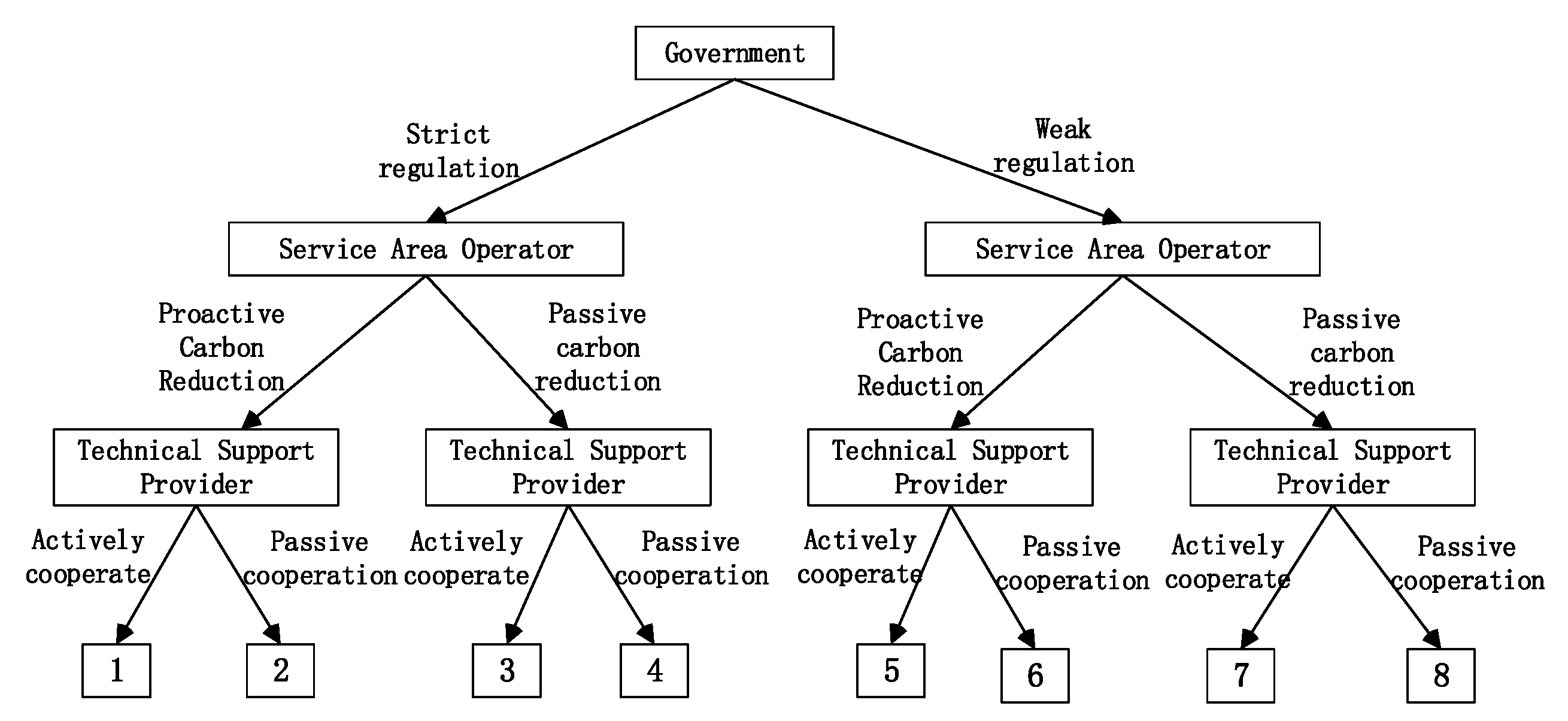
The carbon reduction technical support provider is responsible for the R&D of carbon reduction technologies and economic risk balancing. They address carbon reduction challenges in highway service areas through technological solutions, achieving technical innovations and breakthroughs tailored to Xinjiang, China’s geographical characteristics and environmental particularities, thereby providing technical support for service area carbon reduction. Technical Support Providers may exhibit two behavioral patterns in the game: (1) Active Cooperation: Proactively collaborating with carbon reduction enterprises by providing carbon reduction technologies, including offering low-cost technologies and long-term carbon reduction services for service areas; (2) Passive Cooperation: Engaging in passive collaboration with carbon reduction enterprises, such as offering high-cost technologies and short-term services, without actively promoting carbon reduction progress in service areas. Therefore, the behavioral strategy space for technical support providers is assumed to be S3 = (Active Cooperation, Passive Cooperation), with respective strategy probabilities of z (0 ≤ z ≤ 1) and 1 − z. The corresponding three-party evolutionary game tree model diagram is as Figure 3:

3.1.2. Model Assumptions

Based on key influencing factors for carbon reduction in Xinjiang service areas, this study considers the economic, social, and risk impacts of the three stakeholders. Integrating their interaction mechanisms and dynamic evolutionary logic during carbon reduction, the following assumptions are made, which are grounded in empirical and theoretical foundations:
(1) Bounded Rationality Assumption
Governments, service area operators, and technology providers exhibit bounded rationality that is not uniformly distributed. Governments face limitations in information collection, making it difficult to accurately predict the carbon reduction pathways chosen by service area operators and technology providers, as well as the corresponding effectiveness of carbon reduction technologies. Service area operators face challenges in making optimal decarbonization decisions due to policy directives, market demand pressures, and technology adaptation risks. Technology providers may exhibit uncertainty regarding collaborative proposals and expected returns, constrained by new technology development, technical compatibility, and breakthroughs in key technologies.
(2) Dynamic Strategy Adjustment Assumption
During service area decarbonization, each party dynamically adjusts its strategy based on analysis of the other two parties’ strategy implementation.
(3) Tripartite Benefit and Cost Assumptions
Government benefits encompass economic, social, and environmental gains, while costs include policy formulation, oversight incentives, carbon reduction subsidies, and coordination expenses. Service area operators derive revenue from cost reductions achieved through carbon reduction, with costs comprising technological investment, operational maintenance, management optimization, and compliance expenses. Technology providers gain from technical services, policy incentives, and market expansion opportunities, while costs involve R&D investment, equipment manufacturing/installation, and collaboration risks.
(4) Quantification of Evaluation Values
Throughout the carbon reduction process in service areas, associated costs, benefits, and social impacts are quantifiable, with all exogenous variables exhibiting positive values.

3.2. Establishment of a Tripartite Evolutionary Game Model

The model derivation in this study follows the evolutionary game theory framework proposed by Friedman [41], which integrates classical game theory with dynamic evolutionary processes and is applicable to analyzing the evolutionary group behavior of agents with bounded rationality. The core modeling process comprises: (1) defining agents and strategy spaces; (2) constructing payoff matrices; (3) establishing replicator dynamics equations; and (4) conducting equilibrium stability analysis. This established methodology has been extensively applied in environmental governance and sustainable transition research, providing a robust theoretical foundation for this model’s construction.

3.2.1. Parameter Settings

Combining 15 key influencing factors with the three-party game entities, the parameters are set as detailed in Table 2 below.

3.2.2. Tripartite Evolutionary Game Dynamic Reproduction Equation

The payoff matrix and replicator dynamics equations constructed in this section follow the standard modeling procedures of evolutionary game theory. The payoff matrix is logically derived based on the strategy combinations of the three agents and the model parameters, and its structure represents the standard form for such studies. The replicator dynamics equations for each agent serve as the core analytical tool in evolutionary game theory [42], and thus directly adopt the standard replicator dynamics form from evolutionary game theory. Therefore, the formula represents the specific expression obtained by substituting the particular payoff function defined in this study into this standard equation, rather than a novel formula construction. The innovation of this model lies in applying this standard framework to the specific context of carbon reduction in Xinjiang’s highway service areas and defining a parameter system that reflects the uniqueness of this context.
Based on the model assumptions and parameter settings outlined above, the payoff matrix for the three-party evolutionary game on carbon reduction in Xinjiang’s highway service areas is shown in Table 3.
(1) Let the government’s benefit from adopting strong regulation be Ug1, the benefit from adopting weak regulation be Ug2, and the average expected benefit be Ug. The following formula is derived:
U g 1 = y × z × ( B g C g 3 C g 1 S M ) + y × ( 1 z ) × ( B g C g 3 C g 1 S ) + ( 1 y ) × z × ( B g + F C g 3 C g 1 M ) + ( 1 y ) × ( 1 z ) × ( B g + F C g 3 C g 1 ) = B g C g 3 C g 1 + ( 1 y ) × F y × S z × M
U g 2 = y × z × ( C g 3 C g 2 ) + y × ( 1 z ) × ( C g 3 C g 2 ) + ( 1 y ) × z × ( C g 3 C g 2 ) + ( 1 y ) × ( 1 z ) × ( C g 3 C g 2 ) = C g 3 C g 2
U g = x U g 1 + ( 1 x ) U g 2
The government’s replicating dynamic equation is:
F ( x ) = d x / d t = x × ( U g 1 U g ) = x × ( 1 x ) × [ B g + ( 1 y ) × F C g 1 + C g 2 y × S z × M ]
(2) Let the revenue from proactive carbon reduction measures by the service area operator be denoted as Ue1, and the revenue from reactive carbon reduction measures as Ue2. The average expected revenue is denoted as Ue, yielding the following formula:
U e 1 = x × z × [ k × Re + V + S Ce 4 ( 1 α ) × ( Ce 1 + Ce 3 ) L ] + x × ( 1 z ) × [ k × Re + V + S Ce 4 ( Ce 1 + Ce 3 ) L ] + ( 1 x ) × z × [ k × Re + V Ce 4 ( 1 α ) × ( Ce 1 + Ce 3 ) L ] + ( 1 x ) × ( 1 z ) × [ k × Re + V Ce 4 ( Ce 1 + Ce 3 ) L ] = k × Re + V Ce 4 ( Ce 1 + Ce 3 ) L + x × S + z α × ( Ce 1 + Ce 3 )
U e 2 = x × z × ( C e 4 Ce 2 F L ) + x × ( 1 z ) × ( C e 4 Ce 2 F L ) + ( 1 x ) × z × ( C e 4 Ce 2 L ) + ( 1 x ) × ( 1 z ) × ( C e 4 Ce 2 L ) = C e 4 Ce 2 L x × F
U e = y × U e 1 + ( 1 y ) × U e 2
The replicated dynamic equation for service area operators is:
F ( y ) = d y / d t = y × ( U e 1 U e ) = y × ( 1 y ) × [ k × Re + V + x × ( S + F ) + z × α × ( Ce 1 + Ce 3 ) + Ce 2 ( Ce 1 + Ce 3 ) ]
(3) Let the payoff for the technical support provider choosing active cooperation be Ut1, the payoff for choosing passive cooperation be Ut2, and the average expected payoff be Ut. The following formula is derived:
U t 1 = x × y × ( Q + R t × β + M C t 3 C t 1 ) + x × ( 1 y ) × ( Q + R t + M C t 3 C t 1 ) + ( 1 x ) × y × ( Q + R t × β C t 3 C t 1 ) + ( 1 x ) × ( 1 y ) × ( Q + R t C t 3 C t 1 ) = Q + R t C t 3 C t 1 + y × R t × ( β 1 ) + x × M
U t 2 = x × y × ( Q C t 3 C t 2 ) + x × ( 1 y ) × ( Q C t 3 C t 2 ) + ( 1 x ) × y × ( Q C t 3 C t 2 ) + ( 1 x ) × ( 1 y ) × ( Q C t 3 C t 2 ) = Q C t 3 C t 2
U t = z × ( 1 z ) × [ R t + M C t 1 + C t 2 + y × R t × ( β 1 ) ]
The replication dynamic equation for the technical support provider is:
F ( z ) = d z / d t = z × ( U t 1 U t ) = z × ( 1 z ) × [ y × ( β 1 ) × R t + R t + x × M + C t 2 C t 1 ]

4. Tripartite Evolutionary Game Analysis

4.1. Tripartite Evolutionary Path Analysis

(1) Government Stability Analysis
According to the requirements of the Evolutionarily Stable Strategy (ESS), when F(x) = 0 and F′(x) < 0, the corresponding x represents the government’s evolutionarily stable strategy. The same logic applies to the service area operator and technical support provider, thereby determining the stable strategies for all three parties.
When F(x) = 0, the solutions are x = 0 and x = 1.
z * = ( 1 y ) × F C g 1 + C g 2 y × S M
The derivative of the government’s replicating dynamic equation is as follows:
F ( x ) = ( 1 2 x ) × [ B g + ( 1 y ) × F C g 1 + C g 2 y × S z × M ]
If z = ( 1 y ) × F C g 1 + C g 2 y × S M , then F(x) = 0, and all values of x in this scenario are in an evolutionarily stable state.
If z ( 1 y ) × F C g 1 + C g 2 y × S M , then x = 0 and x = 1 are evolutionary equilibrium points. Let G ( z ) = Bg + ( 1 y ) × F Cg 1 + Cg 2 y × S z × M . Taking the partial derivative of F(x) yields d(F(x))/dx = (1 − 2x)G(z). Since d(G(z))/dz = −M < 0, G(z) is a decreasing function. In this case, the following two situations arise:
Scenario 1: When z   >   ( 1 y ) × F C g 1 + C g 2 y × S M , then G(z) < 0. Simultaneously, for F′(x), F′(1) > 0 and F′(0) < 0. Therefore, x = 0 represents an evolutionarily stable equilibrium point, indicating that when the probability of active cooperation by the technology provider is z   >   ( 1 y ) × F C g 1 + C g 2 y × S M , the government’s regulatory intensity for carbon reduction in the service area tends toward weak regulation.
Scenario 2: When z   <   ( 1 y ) × F C g 1 + C g 2 y × S M , G(z) > 0. Simultaneously, for F′(x), F′(1) < 0 and F′(0) > 0. Therefore, x = 1 represents an evolutionarily stable equilibrium point, indicating that when the probability of active cooperation by the technology provider reaches z   <   ( 1 y ) × F C g 1 + C g 2 y × S M , the government’s regulatory intensity for carbon reduction in the service area tends toward strong regulation.
For the three possible values of z, the corresponding phase diagrams for system stability conditions—that is, the phase diagrams for the evolution of government carbon reduction strategies in Xinjiang highway service areas—are shown in Figure 4 below. Note that the strategy probabilities are dimensionless:
(2) Stability Analysis of Service Area Operator
Similarly, when F(y) = 0 and F′(y) < 0, the corresponding y represents the government’s evolutionarily stable strategy. The same logic applies to the service area operator and technical support provider, thereby determining the stable strategies for all three parties.
When F(y) = 0, the solutions are y = 0 and y = 1.
x * = k × Re V z × α × ( Ce 1 + Ce 3 ) Ce 2 + ( Ce 1 + Ce 3 ) ( S + F )
The derivative of the government’s replicating dynamic equation is as follows:
F ( y ) = ( 1 2 y ) × [ k × Re + V + x × ( S + F ) + z × α × ( Ce 1 + Ce 3 ) + Ce 2 ( Ce 1 + Ce 3 ) ]
If x = k × Re V z × α × ( Ce 1 + Ce 3 ) Ce 2 + ( Ce 1 + Ce 3 ) ( S + F ) , at this point, all y values in this scenario are in an evolutionarily stable state.
If x k × Re V z × α × ( Ce 1 + Ce 3 ) Ce 2 + ( Ce 1 + Ce 3 ) ( S + F ) , then y = 0 and y = 1 are evolutionary equilibrium points. Let H ( x ) = k × Re + V + x × ( S + F ) + z × α × ( Ce 1 + Ce 3 ) + Ce 2 ( Ce 1 + Ce 3 ) , and take the partial derivative of F(y) with respect to y: d(F(y))/dy = (1 − 2y)H(x). Since d(F(x))/dx = S + F > 0 and H(x) is an increasing function, the following two cases arise:
Scenario 1: When x   >   k × Re V z × α × ( Ce 1 + Ce 3 ) Ce 2 + ( Ce 1 + Ce 3 ) ( S + F ) , H(x) > 0. Simultaneously, for F′(y), F′(1) < 0 and F′(0) > 0. Therefore, y = 1 represents an evolutionarily stable equilibrium point, indicating that when the probability of stringent government regulation is x   >   k × Re V z × α × ( Ce 1 + Ce 3 ) Ce 2 + ( Ce 1 + Ce 3 ) ( S + F ) , service area operators will intensify their proactive carbon reduction efforts for highway service areas.
Scenario 2: When x   <   k × Re V z × α × ( Ce 1 + Ce 3 ) Ce 2 + ( Ce 1 + Ce 3 ) ( S + F ) , G(z) is less than 0. Simultaneously, for F′(x), F′(1) > 0 and F′(0) < 0. Therefore, y = 0 represents an evolutionarily stable equilibrium point. This indicates that when the probability of the government imposing stringent regulations on carbon reduction in highway service areas is z < ( 1 y ) × F C g 1 + C g 2 y × S M , the service area operators will increasingly reduce their proactive efforts toward carbon reduction in these areas.
For the three possible values of x, the corresponding phase diagrams of system stability conditions—that is, the phase diagrams of the evolution of operating enterprises’ carbon reduction strategies for Xinjiang highway service areas—are shown in Figure 5 below. The strategy probabilities are dimensionless.
(3) Stability Analysis of the Technical Support Provider
According to the requirements of the Evolutionarily Stable Strategy (ESS), when F(z) = 0 and F′(z) < 0, the corresponding z represents the government’s evolutionarily stable strategy. The same logic applies to the service area operator and the technical support provider, thereby determining the stable strategies for all three parties.
When F(z) = 0, the solutions are z = 0 and z = 1.
y * = R t + x × M + C t 2 C t 1 ( 1 β ) × R t
The derivative of the government’s replicating dynamic equation is as follows:
F ( z ) = ( 1 2 z ) × [ y × ( β 1 ) × R t + R t + x × M + C t 2 C t 1 ]
If y = R t + x × M + C t 2 C t 1 ( 1 β ) × R t , then F(z) = 0, and all values of z in this scenario are in an evolutionarily stable state.
If y R t + x × M + C t 2 C t 1 ( 1 β ) × R t , then z = 0 and z = 1 are evolutionary equilibrium points. Let K ( y ) = y × ( β 1 ) × R t + R t + x × M + C t 2 C t 1 , and take the partial derivative of F(z) with respect to z: d(F(z))/dz = (1 − 2x)K(z). Since d(K(y))/dy = (β − 1)Rt > 0 and K(y) is an increasing function, the following two cases arise:
Scenario 1: When y   >   R t + x × M + C t 2 C t 1 ( 1 β ) × R t , F′(0) > 0. Therefore, z = 1 represents an evolutionarily stable equilibrium point. This indicates that as the probability of service area operators actively reducing carbon emissions increases y > R t + x × M + C t 2 C t 1 ( 1 β ) × R t , the probability of technical support providers cooperating proactively in carbon reduction efforts at highway service areas also increases.
Scenario 2: When y < R t + x × M + C t 2 C t 1 ( 1 β ) × R t , K(y) < 0. Simultaneously, for F′(x), F′(1) > 0 and F′(0) < 0. Therefore, z = 0 represents an evolutionarily stable equilibrium point, indicating that when the probability of service area operators actively reducing carbon emissions is y < R t + x × M + C t 2 C t 1 ( 1 β ) × R t , the probability of technical support providers cooperating proactively in carbon reduction efforts at highway service areas decreases.
For the three scenarios of y values, the corresponding phase diagrams of system stability conditions—that is, the evolution phase diagrams of carbon reduction strategies provided by the technical support team for Xinjiang highway service areas—are shown in Figure 6 below. Note that the strategy probabilities are dimensionless.

4.2. Tripartite Evolutionary Stability Analysis

According to Jacobian matrix theory, setting the replication dynamics equations for all three parties to zero yields eight pure strategy equilibrium points for this three-party evolutionary game: E1 (0,0,0), E2 (0,0,0), E3 (0,0,1), E4 (0,1,1), E5 (1,0,0), E6 (1,1,0), E7 (1,0,1), E8 (1,1,1). To determine the stability of these equilibrium points, the first Lyapunov method is applied [43]. The Jacobian matrix is constructed as follows:
J = a 11 a 12 a 13 a 21 a 22 a 23 a 31 a 32 a 33 = F ( x ) x F ( x ) y F ( x ) z F ( y ) x F ( y ) y F ( y ) z F ( z ) x F ( z ) y F ( z ) z
The values of each element in the matrix are as follows:
a 11 = F ( x ) x = ( 1 2 x ) × [ Bg + ( 1 y ) × F Cg 1 + Cg 2 y × S z × M ] a 12 = F ( x ) y = x × ( 1 x ) × ( F S ) a 13 = F ( x ) z = M × x × ( 1 x ) a 21 = F ( y ) x = y × ( 1 y ) × ( S + F ) a 22 = F ( y ) y = ( 1 2 y ) × [ k × Re + V + x × ( S + F ) + z × α × ( Ce 1 + Ce 3 ) + Ce 2 ( Ce 1 + Ce 3 ) ] a 23 = F ( y ) z = α × y × ( 1 y ) × ( Ce 1 + Ce 3 ) a 31 = F ( z ) x = M × z × ( 1 z ) a 32 = F ( z ) y = z × ( 1 z ) × ( β 1 ) × Rt a 33 = F ( z ) z = ( 1 2 z ) × [ y × ( β 1 ) × Rt + Rt + x × M + Ct 2 Ct 1 ]
If all three eigenvalues of an equilibrium point are negative, it is an evolutionary equilibrium point; if all are positive, it is an unstable point; if one or two are positive, it is a saddle point. Based on the Jacobian matrix, substituting the equilibrium point yields the corresponding eigenvalues and stability conditions shown in Table 4.
As shown in the table above, E7 does not satisfy Lyapunov stability theory. For the remaining seven equilibrium points to become ESS stable points, they must satisfy the corresponding stability conditions listed in the table.

5. Simulation Analysis of Tripartite Evolutionary Games

The ideal stable equilibrium point achievable in the tripartite evolutionary game for carbon reduction in service areas, which holds practical significance, is E8 (1,1,1), i.e., (strong regulation, active carbon reduction, active cooperation). This study employs MATLAB R2020a for numerical simulation analysis. All simulations are conducted based on the aforementioned replicator dynamics equations and baseline parameter set to investigate the influence of various factors on the strategic behaviors of the three parties. The simulation code is detailed in Appendix A. To enhance the scientific rigor and credibility of model parameter assignments, ensuring greater alignment with Xinjiang’s actual conditions, this study employed structured expert interviews to determine baseline values for model parameters. All parameters underwent normalization and were incorporated into the model as relative values for simulation analysis. The core objective was to examine the model’s intrinsic mechanisms and strategic evolution trends rather than conducting precise numerical predictions. Fifteen experts from relevant fields participated in the interviews, forming a well-structured decision-making advisory team: 6 senior-level professionals, 6 associate senior-level professionals, and 3 intermediate-level professionals. Six experts held doctoral degrees, five held master’s degrees, and four held bachelor’s degrees, ensuring a solid theoretical foundation and rich practical experience. Six experts hailed from Xinjiang’s new energy research institutions, six from ecological and geographical research units, and three from energy development organizations. All experts possess long-term dedication to research or practice in the energy, environment, and transportation fields in Xinjiang, demonstrating profound understanding and firsthand experience with the region’s unique context: a vast territory with a sparse population, remote grid peripheries, extreme climates, and abundant clean energy resources yet high curtailment rates.
The interviews employed a combination of semi-structured interviews and the Delphi method. First, the research team provided the expert panel with a detailed introduction to the three-party evolutionary game model developed for this study, explaining the definition and economic implications of each parameter within the game. Subsequently, experts were asked to independently assess reasonable parameter ranges based on their professional judgment and local experience. For parameters with significant divergence, up to two rounds of back-to-back anonymous feedback were conducted until a consensus emerged. The final parameter values are presented in Table 5 below:

5.1. Simulation of the Tripartite Evolutionary Pathway

By combining the simulation parameter values from the previous group with different initial strategies and evolving them over time, the initial evolutionary path diagram shown in Figure 7 was obtained.
As shown in Figure 4, the three-party evolutionary game system possesses a unique evolutionary stable strategy (ESS) = (1,1,1). Although the convergence speeds of the three strategies are inconsistent, they ultimately converge to the Pareto optimal state of ESS = (1,1,1).

5.2. Simulation of the Impact of Initial Value Changes on Evolutionary Outcomes

The three-dimensional and two-dimensional simulation diagrams illustrating the impact of initial value changes in x, y, and z—i.e., the three variables—on the final evolutionary outcome are shown in Figure 8.
It can be observed that over time, x, y, and z all evolve toward 1. Concurrently, the evolution rate of x (the government) exceeds that of y (the service area operator), which in turn exceeds that of z (the technical support provider). This indicates that during the carbon reduction process for service areas, the government’s strategic choices exert the most significant driving force on the system, followed by the service area operator. Meanwhile, the technical support provider tends to adopt a more cautious approach in carbon reduction decisions, requiring a longer observation period to assess benefits and risks before adjusting strategies.
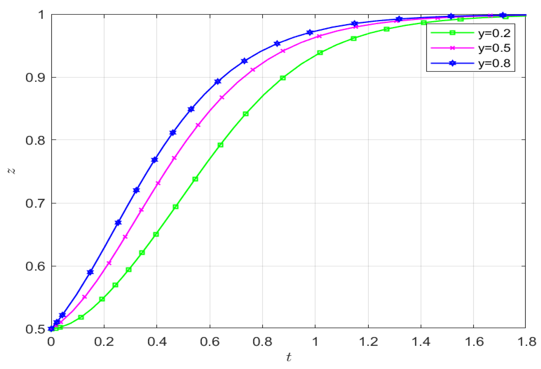
As shown in Figure 9, increasing the initial value of x exerts a positive incentive effect on service area operators to actively reduce carbon emissions. At this point, the system converges more rapidly to an evolutionary stable state, with the final equilibrium time consistently clustering around 1.35.
As shown in Figure 10, increasing the initial value of government regulatory intensity x exerts a positive incentive effect on the active cooperation of carbon reduction technology support providers in service areas. At this point, a shorter time is required to reach an evolutionary stable state, with the final stable time consistently clustering around 1.7.
As shown in Figure 11, increasing the baseline value of the service area operator’s proactive carbon reduction efforts exerts a positive incentive effect on the active cooperation of technical support providers for carbon reduction. This facilitates greater engagement from technical support providers, with the stabilization time ultimately clustering around 1.7.

5.3. Parameter Sensitivity Simulation

(1) Simulation Analysis of Government Regulation Impact on Service Area Carbon Reduction Strategies
(1) Incremental Costs Cg1 Under Strong Government Regulation
Cg1 is set at three distinct levels: low investment (Cg1 = 2.5), medium investment (Cg1 = 5), and high investment (Cg1 = 10). With all other parameters held constant, the simulations are conducted and the results are shown in Figure 12.
As shown in the figure, the smaller the Cg1 value, the earlier the government stabilizes at the equilibrium state ESS (1,1,1). The earliest stabilization time is 0.6, while the latest is 2, representing an extension of 233.3%. For service area operators, stabilization occurs at 1.3 regardless of parameter values, and their willingness to actively reduce carbon emissions decreases as parameter values increase. Technical support providers converge toward stability at 1.7 under all parameter settings, with their willingness to actively cooperate in carbon reduction decreasing as Cg1 increases. Consequently, the government exhibits heightened sensitivity to cost changes under stringent regulation. Higher costs reduce the government’s available subsidy funds, leading to a delayed decision to adopt “strong regulation.”
(2) Environmental governance costs incurred by the government under weak regulation (Cg2)
Cg2 is set at three distinct levels: low investment (Cg2 = 4), medium investment (Cg2 = 8), and high investment (Cg2 = 16). With all other parameters held constant, the simulations are conducted and the results are shown in Figure 13.
As shown in the figure, the larger the value of Cg2, the sooner the government evolves toward equilibrium, with the earliest stabilization occurring at 0.4 and the latest at 1.4. For the operating company, stabilization is achieved at 1.3 regardless of parameter values, and proactive carbon reduction willingness increases as the parameter value grows. For the technology provider, stability is achieved at Cg2 values of 1.7, with increased willingness to cooperate on carbon reduction as the parameter rises. Consequently, the government exhibits high sensitivity to environmental governance costs incurred under weak regulation. Rising environmental costs compel the government to strengthen oversight to avoid long-term environmental burdens, thereby indirectly boosting the willingness of enterprises and technology providers to collaborate on carbon reduction.
(3) Additional subsidy amount S for enterprises’ “proactive carbon reduction” under strong government regulation
Setting S at three distinct levels: low subsidy (S = 1.5), medium subsidy (S = 3), and high subsidy (S = 6), while keeping other parameters constant, numerical simulations were conducted using MATLAB. The results are shown in Figure 14.
As shown in the figure, at different S value levels, the smaller the S value, the sooner the government evolves toward equilibrium, stabilizing as early as 0.5 and as late as 1. Operating enterprises stabilize as early as 0.8 and as late as 1.6, with their willingness to proactively reduce carbon emissions increasing as the value rises. Technical support providers stabilize at S = 1.6 regardless of parameter variations. Consequently, both the government and service area operators exhibit high sensitivity to changes in additional subsidies for “proactive carbon reduction” under stringent government regulation. Excessive subsidies increase fiscal pressure, delaying the stabilization of government strategies. Simultaneously, subsidies directly offset enterprises’ equipment investment costs for carbon reduction, boosting their initiative and thereby increasing demand for collaboration with technical providers.
(4) Additional subsidy M provided by the government under strong regulatory conditions to incentivize technology providers’ active carbon reduction development cooperation
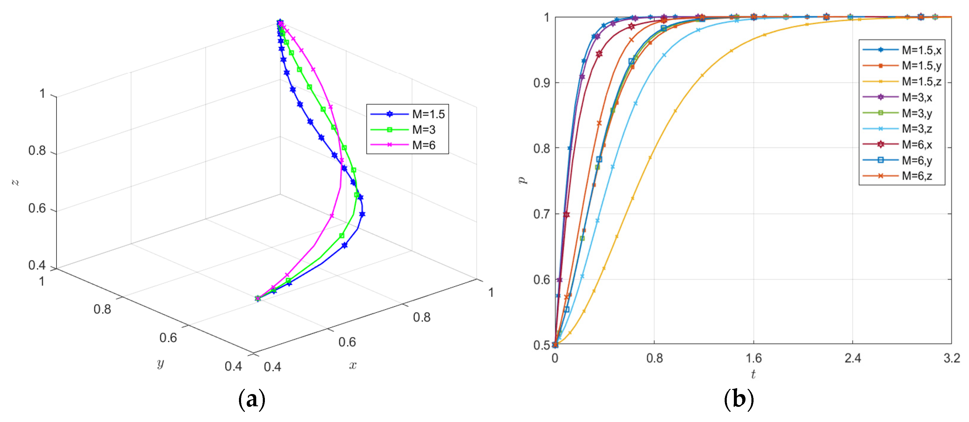
Setting M at three distinct levels: low subsidy (M = 1.5), medium subsidy (M = 3), and high subsidy (M = 6), while keeping other parameters constant, yields the simulation results shown in Figure 15.
As shown in the figure, at different M values, the larger the M value, the slower the government’s evolution toward equilibrium. It stabilizes at 0.6 at the earliest and at 1 at the latest. Service area operators show little variation, all stabilizing at 1.2. Technical support providers stabilize at 1 at the earliest and at 2.8 at the latest, with faster convergence toward stability as M increases. Therefore, technical support providers exhibit greater sensitivity to additional subsidies offered by the government for proactive low-carbon development cooperation under stringent regulatory conditions. These subsidies can be directly applied to R&D for sandstorm resistance, low-temperature tolerance, and energy storage optimization, thereby enhancing market competitiveness and risk resilience. Simultaneously, this increases fiscal pressure on the government and prolongs decision-making timelines.
(5) Positive social benefits (Bg) from government strong regulation
Bg is set at three levels: low benefit (Bg = 5), medium benefit (Bg = 10), and high benefit (Bg = 20). With the other parameters held constant, simulations are conducted and the results are shown in Figure 16.
As shown in the figure, at different Bg values, the larger the value, the earlier the government evolves toward equilibrium with noticeable changes, with the earliest trending toward policy stability at 0.4 and the latest at 1.8. Service area operators tend toward stability at 1.3 for all values, and the higher the parameter value, the greater the willingness to stabilize. Technical support providers stabilize at 1.6, with their willingness to cooperate increasing as Bg rises. Therefore, the government exhibits high sensitivity to Bg—the positive social benefits derived from stringent regulation—which also positively influences the other two parties. For instance, achieving regional carbon reduction targets and enhancing public satisfaction with green transportation strengthen the government’s regulatory motivation, fostering a virtuous cycle of “enhanced regulation → corporate response → technological cooperation.”
(6) Government Strong Regulation on Enterprise “Passive Carbon Reduction” Penalty F
Setting F at three distinct levels: low penalty (F = 1), medium penalty (F = 2), high penalty (F = 4), while keeping the other parameters constant, yields simulation the results shown in Figure 17.
As shown in the figure, at different levels of F, the higher the value, the less significant the changes in government and technical support providers. The decision-making time for service area operators to proactively reduce carbon emissions shortens, stabilizing as early as 1 and as late as 1.6. Therefore, service area operators exhibit high sensitivity to penalty F imposed by stringent government regulation for “passive carbon reduction.” Since penalties directly increase the cost of passive carbon reduction, they compel enterprises to shift toward proactive carbon reduction. However, this has no direct impact on government or technology providers.
(2) Simulation Analysis of Service Area Operators’ Strategy Impacts from Implementing Carbon Reduction Measures
(1) Investment Costs Ce1 for Equipment and Technology in “Proactive Carbon Reduction”
Ce1 was set at three distinct levels: low cost (Ce1 = 2), medium cost (Ce1 = 4), and high cost (Ce1 = 8). With the other parameters held constant, simulations are conducted and the results are shown in Figure 18.
As shown in the figure, at different Ce1 values, the greater the value, the less the government’s response changes. Service area operators stabilize at 1 at the earliest and at 2.2 at the latest, with stabilization slowing as the parameter increases. Technical support providers stabilize at 1.8, and as Ce1 increases, their willingness to actively cooperate on carbon reduction rises without significant variation. Therefore, service area operators exhibit high sensitivity to changes in investment costs for equipment and technology associated with “proactive carbon reduction.” Significant upfront expenditures—such as procurement costs for low-carbon heating systems and new energy charging stations—substantially reduce enterprises’ expectations for cost recovery from carbon reduction efforts, thereby diminishing the demand for customized technologies from technical partners.
(2) Enterprise “Passive Carbon Reduction” Costs Ce2
Ce2 was set at three distinct levels: low cost (Ce2 = 0.5), medium cost (Ce2 = 1), and high cost (Ce2 = 2). With the other parameters held constant, simulations are conducted and the results are shown in Figure 19.
As shown in the figure, at different Ce2 values, the greater the value, the less significant the changes in government and technical support providers. Service area operators tend to stabilize at Ce2 = 1.3, and as Ce2 increases, their willingness to proactively reduce carbon emissions rises. Therefore, changes in the cost of “passive carbon reduction” (Ce2) for enterprises show a positive correlation with the enthusiasm for carbon reduction among operators. However, it has little impact on the time required for final decision stability. Due to the low baseline cost of passive carbon reduction, even when costs increase, the driving effect on corporate strategy selection remains limited.
(3) Subsequent maintenance costs for “proactive carbon reduction” Ce3
Ce3 was set at three distinct levels: low cost (Ce3 = 0.5), medium cost (Ce3 = 1), and high cost (Ce3 = 2). With the other parameters held constant, simulations are conducted and the results are shown in Figure 20.
As shown in the figure, the government and technology support providers exhibit little variation across the different Ce3 levels. Service area operators stabilize at 1.4 when parameters change, and their proactive carbon reduction willingness decreases as Ce3 increases. Therefore, when the subsequent maintenance costs of “proactive carbon reduction” increase, the willingness to reduce emissions decreases, while the stability time of the strategy remains largely unchanged. This is because the baseline costs of passive carbon reduction are low, limiting their driving effect on corporate strategy selection.
(4) Economic savings and benefits from enterprises’ “proactive carbon reduction,” such as energy cost savings and new energy generation revenue, are represented by Re
Re is set at three different levels: low benefit (Re = 0.5), medium benefit (Re = 1), and high benefit (Re = 2). With the other parameters held constant, simulations are conducted and the results are shown in Figure 21.
As shown in the figure, the government and technology support providers exhibit little variation across different Re value levels. Service area operators stabilize at Re = 1.3, and their willingness to proactively reduce carbon emissions increases as the parameter rises. Consequently, while greater economic savings and benefits from voluntary carbon reduction boost corporate enthusiasm, this has limited impact on stabilization time. This is because Xinjiang’s policy framework for surplus electricity grid injection and supply to neighboring regions remains underdeveloped, yielding constrained economic returns.
(5) The elasticity coefficient k of corporate voluntary carbon reduction efforts on returns
k is set to three distinct levels: low elasticity (Re = 0.5), medium elasticity (Re = 1), and high elasticity (Re = 2). With all the other parameters held constant, simulations are conducted and the results are shown in Figure 22.
As shown in the figure, changing the values of k resulted in little change in the behavior of governments and technology providers. Service area operators tend to stabilize at k = 1.4, and their willingness to proactively reduce carbon emissions increases as the parameter grows. This occurs because most service areas in Xinjiang operate as independent energy units, making it difficult for individual enterprises’ voluntary carbon reduction efforts to yield economies of scale. Consequently, the driving effect of k on stabilization time is constrained, explaining why k only influences the intensity of willingness rather than altering the time required for strategy stabilization.
(6) Potential income V derived from brand premiums and other benefits resulting from enterprises’ “proactive carbon reduction”
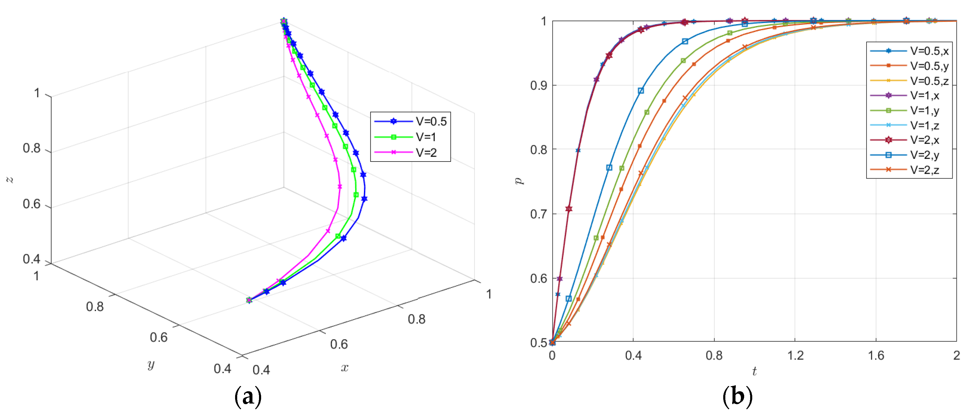
V is set at three distinct levels: low income (V = 0.5), medium income (V = 1), and high income (V = 2). With the other parameters held constant, simulations are conducted and the results are shown in Figure 23.
As shown in the figure, the potential revenue V generated by enterprises’ “proactive carbon reduction” efforts—such as brand premiums—causes minimal changes to government and technology provider stabilization strategies across different parameter values. Service area operators demonstrate increased enthusiasm for proactive carbon reduction as parameters rise, ultimately stabilizing at 1.3. Therefore, as the value of potential income from brand premiums and other benefits derived from “proactive carbon reduction” increases, companies’ willingness to reduce emissions rises. However, this has little impact on the final stabilization time. This is because brand premiums represent indirect benefits, exerting weaker driving effects on companies’ short-term carbon reduction decisions compared to direct economic gains.
(7) Coefficient β of Enterprise “Proactive Carbon Reduction” on Technology Provider Revenue Enhancement
Setting β at three distinct levels: low enhancement coefficient (β = 1.1), medium enhancement coefficient (β = 2), and high enhancement coefficient (β = 4), while the keeping other parameters constant, yields the simulation results shown in Figure 24.
As shown in the figure, the coefficient β representing the increase in benefits for technology providers due to enterprises’ “proactive carbon reduction” remains relatively stable across different parameter values, regardless of government and enterprise strategy. As the parameter value increases, the willingness of technology providers to engage in proactive carbon reduction cooperation rises, with the earliest stabilization time occurring at 1 and the latest at 4.5. Therefore, technology providers exhibit sensitivity to changes in the coefficient β reflecting the enhancement of their benefits from enterprises’ proactive carbon reduction efforts. This reflects the positive impact of such initiatives on technology providers’ returns: a higher coefficient translates to greater benefits for technology providers from the collaboration and stronger cooperation willingness.
(3) Simulation Analysis of Technology Supporters’ Influence on Service Area Carbon Reduction Collaboration Strategies
(1) Additional costs incurred by technology providers for proactive cooperation, including customized R&D, microgrid adaptation, and breakthroughs in energy storage technology development (Ct1)
Ct1 was set at three distinct levels: low cost (Ct1 = 5), medium cost (Ct1 = 10), and high cost (Ct1 = 20). With all the other parameters held constant, simulations are conducted and the results are shown in Figure 25.
The three-dimensional diagram shows that when Ct1 is set to 5 or 10, the three-party evolutionary game ultimately converges toward ESS (1,1,1). When Ct1 increases to 20, the final outcome evolves toward (1,1,0), indicating that the technical support provider becomes less inclined to actively cooperate at this point. The two-dimensional diagram shows that the technology supporter stabilizes at 0.6 under all parameter values. For the service area operator, willingness to proactively reduce carbon emissions decreases as parameter values increase, with the earliest stabilization occurring at 1.2 and the latest at 2. For the technical support provider, when Ct1 is set to 5 and 10, the final equilibrium evolves toward 1, with smaller values indicating greater willingness to actively cooperate. The stabilization times are 0.8 and 1.6, respectively. When Ct1 increases to 20, the high additional costs exceed the benefits of cooperation, leading to a strategic shift by the technical provider. Simultaneously, rising costs prompt the technology provider to increase cooperation bids, thereby reducing enterprises’ willingness to proactively reduce carbon emissions. Consequently, both the technology provider and operating enterprises exhibit high sensitivity to this factor.
(2) Opportunity cost losses, reputational damage, and market risk costs incurred by the technology provider’s passive cooperation (Ct2)
Ct2 was set at three distinct levels: low loss (Ct2 = 2.5), medium loss (Ct2 = 5), and high loss (Ct2 = 10). With the other parameters held constant, simulations are conducted and the results are shown in Figure 26.
As shown in the figure, changing the loss Ct2 resulting from the technical support provider’s passive cooperation causes minimal variation in the stabilization time of government and operator strategies across different parameter values. As the parameter value increases, the technology provider’s willingness to proactively reduce carbon emissions rises, with the earliest stabilization occurring at 1 and the latest at 4.5. Consequently, the technology provider is highly sensitive to changes in the Ct2 loss value resulting from passive cooperation. The escalating losses compel the technology provider to shift toward active cooperation, thereby delivering superior technical support to the enterprise.
(3) Incremental benchmark gains Rt from the technology provider’s “proactive cooperation”
Rt is set at three distinct levels: low increment (Rt = 1.5), medium increment (Rt = 3), and high increment (Rt = 6). With the other parameters held constant, simulations are conducted and the results are shown in Figure 27.
As shown in the figure, changing the benchmark incremental benefit Rt resulting from the technical support provider’s “active cooperation” causes minimal variation in the strategy stabilization time for both the government and the operating enterprise across different value levels. The willingness of the technical support provider to actively cooperate is positively correlated with parameter values, with the earliest strategy stabilization occurring at 1 and the latest at 6. Therefore, the technical support provider is highly sensitive to changes in the incremental baseline benefits resulting from “active cooperation.” These incremental benefits directly enhance the economic viability of cooperation, serving as the core driver for the technical provider’s active participation in carbon reduction efforts.
(4) Cost Reduction Coefficient α of “Active Cooperation” by Technology Supporters
Setting α at three distinct levels—low reduction coefficient (α = 0.25), medium reduction coefficient (α = 0.5), and high reduction coefficient (α = 0.9)—while fixing the other parameters, yields the simulation results shown in Figure 28.
As shown in the figure, changing the coefficient α representing the reduction in corporate costs due to the “active cooperation” of the technical support provider causes minimal variation in the stabilization time of government and technical support strategies across different parameter values. For service area operators, the willingness to pursue voluntary carbon reduction increases with higher parameter values, with the earliest stabilization time occurring at 1 and the latest at 1.6. Therefore, service area operators exhibit heightened sensitivity to the coefficient α representing the cost reduction effect of the technical support provider’s “proactive cooperation.” As the technical provider’s carbon reduction technologies tailored to Xinjiang’s regional conditions yield more significant reductions in equipment investment and operational maintenance costs, they directly offset the cost pressures associated with voluntary carbon reduction. This substantially improves cost recovery expectations, thereby accelerating the shift toward a “proactive carbon reduction” strategy. Although the technical provider’s strategic direction remains unchanged, the strength of their cooperative bond with enterprises is indirectly enhanced.

5.4. Limitations and Generalizability of Models

(1) Model Limitations
The simulation results are based on parameter benchmarks determined through expert interviews, and parameter variations may affect evolutionary trajectories and stabilization times. The model relies on key assumptions such as “bounded rationality,” whereas real-world decision-making may be more complex, influenced by non-economic factors like organizational culture and individual leadership preferences. The current lack of empirical comparison with precise historical data limits the model’s predictive accuracy to some extent.
(2) General Applicability Beyond China
The tripartite game analysis framework—involving government, enterprises, and technology providers—developed in this study possesses universal applicability. As these three core stakeholders are central to green transportation infrastructure transitions globally, the framework serves as a versatile analytical tool. While the framework is universal, simulation outcomes—such as which actor exhibits strongest driving force or which parameters are most sensitive—depend on specific institutional environments and regional characteristics. For instance, in European nations with stringent environmental regulations and mature carbon markets, the cost of government “strong regulation” (Cg1) may be low, while penalties (F) and reputational damage (V) from enterprises’ “passive decarbonization” could be high, potentially making enterprises more proactive drivers.
For regions similar to Xinjiang—sparsely populated, vast in area, rich in wind and solar resources but with weak power grids, such as Australia’s interior or certain Middle Eastern countries—many conclusions from this study hold high reference value. These include leveraging distributed renewable energy and addressing extreme environmental adaptation challenges for technology providers. For developing countries where government subsidies S and M may be limited, the “cost threshold” effect revealed by the model becomes even more critical, necessitating exploration of more market-mechanism-based cooperative models.
Thus, this study’s significance lies in providing a replicable analytical framework and a set of key impact parameters. When applying this model to other regions, researchers must recalibrate its parameters based on local policies, market conditions, and economic-technical circumstances to derive region-specific evolutionary pathways and policy implications.

5.5. Model Validation and Robustness

To assess the validity and reliability of this model, the study employs the following three methods for cross-validation, demonstrating the robustness and interpretability of the model results from multiple dimensions.
(1) Theoretical Consistency Test
The stability analysis in this study strictly adheres to standard methods in evolutionary game theory (Friedman, 1998; Weibull, 1995), mathematically deriving the parameter conditions for achieving stability at different equilibrium points through the Jacobian matrix and the first Lyapunov method. This analytical validation ensures the theoretical rigor of the model dynamics. Furthermore, the sensitivity analysis in Section 4 demonstrates that all parameter variations yield responses consistent with economic intuition and managerial common sense, providing strong evidence for the model’s sound construction and logical coherence.
(2) Parameter Robustness Testing (Sensitivity Validation)
Comprehensive parameter sensitivity analysis serves as a critical robustness test. The results indicate:
Within a reasonable neighborhood of the benchmark parameters, the system consistently converges to the ideal ESS (1,1,1) state, demonstrating equilibrium stability. The model successfully identifies critical parameter threshold ranges influencing system evolution. When parameters exceed these thresholds, the system undergoes logical, nonlinear jumps at stability points, demonstrating the model’s ability to accurately capture critical phenomena in real-world decision-making rather than unconditional convergence.
(3) Reality Consistency Test
As Xinjiang’s highway service area systemic carbon reduction practices remain in their early stages, large-sample historical data for quantitative calibration is lacking. Therefore, we employed a reality consistency test as a quasi-empirical validation method, cross-referencing simulation results with qualitative realities, policy documents, and expert knowledge. The simulation results indicate that government strategies converge fastest and exert the strongest driving force, aligning closely with China’s governance system in ecological conservation—characterized by “government leadership, enterprise responsibility, and public participation”. The simulations reveal that corporate behavior is highly sensitive to initial equipment investment, precisely reflecting the core obstacle to carbon reduction investment among Xinjiang service area operators—namely, “significant upfront investment and long return cycles”—consistent with our preliminary research findings. We presented key simulation evolution pathways and conclusions for feedback and discussion during expert interviews. The 15 invited domain experts generally agreed that the model’s evolutionary trends and the relative paces of various actors’ behaviors align with their understanding and assessments of the local conditions in Xinjiang.
Through cross-validation comparing theoretical consistency, parameter robustness, and real-world alignment, this model’s validity, robustness, and explanatory power are strongly supported. Despite limitations such as a lack of large-sample historical data calibration, the above work ensures the reliability of the model conclusions to a significant degree, thereby providing a solid theoretical basis for subsequent policy recommendations.

6. Conclusions and Policy Implications

6.1. Conclusions

This study constructs a tripartite evolutionary game model involving government, enterprises, and technology providers to reveal the collaborative mechanisms of carbon reduction systems in Xinjiang’s highway service areas. The key findings are as follows:
(1) The government serves as the key navigator in system evolution. Its strategy converges most rapidly, driving the entire system through a triple mechanism of “cost-benefit-incentive.” This aligns with findings in most environmental governance literature [44,45,46], but this study further quantifies its transmission effect, demonstrating that enhanced government regulatory intent significantly shortens the decision-making lag period for enterprises and technology providers.
(2) Enterprise behavior is strictly constrained by the “carbon reduction-cost-benefit” balancing mechanism. High equipment investment (Ce1) for proactive carbon reduction is the core barrier, while economic benefits (Re, k) have limited driving force due to constraints from surplus electricity feed-in policies. This finding complements existing research, which often emphasizes technological gains while underestimating institutional barriers to realizing benefits in “grid periphery” regions.
(3) Technology providers act as “threshold decision-makers” in this coordination. Their behavior is driven by “incremental baseline returns (Rt) + scale-driven return enhancement (β)” and exhibits explicit cost thresholds. This represents a novel insight compared to traditional government-enterprise dual-agent models [47,48]. The dual-subject model fails to capture the “cost threshold effect” and “enabling effect (α)” arising from the technology provider’s endogenous strategy. This three-party interaction is precisely the key to overcoming the challenge of “technology deployment difficulties.”

6.2. Policy Implications

(1) Government Level: Implement zoned smart regulation by grouping adjacent, similar service areas into “unified regulatory zones.” Establish a carbon and energy consumption monitoring platform with standardized accounting criteria, linking carbon reduction performance to subsidies and tax incentives to enhance efficiency and reduce costs. Streamline carbon reduction revenue channels by coordinating with power grids to simplify surplus solar power grid-feeding procedures for service areas. Promote the inclusion of emission reductions into carbon credit systems or trading mechanisms to boost enterprises’ green electricity revenues. Establish a technology adaptation initiative, launching the “Xinjiang Special Environment Transportation Carbon Reduction Technology Breakthrough Program.” Utilize dedicated fiscal funds and green credit interest subsidies to support R&D of technologies adapted to windstorms/extreme cold, reducing technical providers’ costs and risks.
(2) Service Area Operator Level: Prioritize investments in high-return projects like “PV + energy storage” and building energy retrofits. Use initial returns to fund deep carbon reduction efforts, mitigating high upfront costs. Expand “Service Area Plus” business models by integrating Xinjiang’s tourism resources to create themed service areas. Combine carbon reduction facilities with landscapes, local specialties, and science education to generate non-electricity revenue streams. Establish a “Green Procurement Alliance” for bulk purchasing of carbon reduction equipment to reduce costs. Jointly submit demand proposals to technology providers to share R&D expenses.
(3) Technology Support Providers: Innovate “energy cost management” and “energy performance contracting” models to invest in, build, and operate facilities, recouping costs through energy savings to alleviate initial investment concerns. Provide end-to-end “design-build-operate-optimize” services, ensuring stable revenue growth and risk mitigation through intelligent operations. Participate in standard-setting and financial innovation, leading the development of western China’s carbon reduction technology standards while leveraging green bonds and credit financing to reduce costs and expand market reach.

Author Contributions

Data curation, H.B.; Funding acquisition, D.Q.; Methodology, H.B.; Supervision, D.Q.; Writing—original draft, H.B. All authors have read and agreed to the published version of the manuscript.

Funding

This research was supported by the Xinjiang Uygur Autonomous Region Key Talent Cultivation Program for Agriculture, Rural Areas, and Farmers (Project No.: 2024SNGGNT063).

Institutional Review Board Statement

Not applicable.

Informed Consent Statement

Not applicable.

Data Availability Statement

The original contributions presented in this study are included in the article. Further inquiries can be directed to the corresponding author.

Conflicts of Interest

The authors declare no conflicts of interest.

Appendix A. MATLAB Simulation Code and Parameter Table (Full Versions of All Code Are Available from the Authors)

(1) Simulation Code for the Tripartite Evolutionary Pathway
%Main Function
function dydt=fuwuqujiangtan(t,y)
  • Cg1 = 5; Cg2 = 8; S = 3; M = 3; Bg = 10; F = 2; Ce1 = 4; Ce2 = 1; Ce3 = 1; Re = 1; k = 1; V = 1; Ct1 = 10; Ct2 = 5; Rt = 3; arf = 0.5; bta = 2;
  • dydt=zeros(3,1);
  • dydt(1) = −y(1)*(y(1) − 1)*(Bg+(1 − y(2))*F − Cg1+Cg2 − y(2)*S − y(3)*M);
  • dydt(2) = −y(2)*(y(2) − 1)*(Re*k+V+y(1)*(S+F)+y(3)*arf*(Ce1+Ce3)+Ce2 − (Ce1+Ce3));
  • dydt(3) = −y(3)*(y(3) − 1)*(y(2)*(bta − 1)*Rt+Rt+y(1)*M+Ct2 − Ct1);
end
clear;clc;
for i = 0.1:0.2:0.9%x
for j = 0.1:0.2:0.9%y
for k = 0.1:0.2:0.9%z
[t,y] = ode45(‘fuwuqujiangtan’,[0 5],[i j k]);
plot3(y(:,1),y(:,2),y(:,3));
xlabel(‘x’);ylabel(‘y’);zlabel(‘z’);
grid on;
hold on
axis([0 1 0 1 0 1]);
end
(2) Simulation Code for the Impact of Initial Value Changes on Evolutionary Outcomes
function dydt=fuwuqujiangtana(t,y,Cg1,Cg2,S,M,Bg,F,Ce1,Ce2,Ce3,Re,k,V,Ct1,Ct2,Rt,arf,bta)
  • dydt = zeros(3,1);
  • dydt(1) = −y(1)*(y(1) − 1)*(Bg+(1 − y(2))*F − Cg1+Cg2 − y(2)*S − y(3)*M);
  • dydt(2) = −y(2)*(y(2) − 1)*(Re*k+V+y(1)*(S+F)+y(3)*arf*(Ce1+Ce3)+Ce2 − (Ce1+Ce3));
  • dydt(3) = −y(3)*(y(3) − 1)*(y(2)*(bta − 1)*Rt+Rt+y(1)*M+Ct2 − Ct1);
  • clc,clear;
  • Cg1 = 5; Cg2 = 8; S = 3; M = 3; Bg = 10; F = 2; Ce1 = 4; Ce2 = 1; Ce3 = 1; Re = 1; k = 1; V = 1; Ct1 = 10; Ct2 = 5; Rt = 3; arf = 0.5; bta = 2;
[t,y] = ode45(@(t,y) fuwuqujiangtana(t,y,Cg1,Cg2,S,M,Bg,F,Ce1,Ce2,Ce3,Re,k,V,Ct1,Ct2,Rt,arf,bta),[0 10],[0.5 0.5 0.5]);
plot(t,y(:,1),’bh-‘,t,y(:,2),’rs-‘,t,y(:,3),’go-‘,’linewidth’,1,’markersize’,4,’MarkerIndices’,1:2:length(t));
hold on;
grid on
xlabel(‘$t$’,’interpreter’,’latex’,’Rotation’,0);
ylabel(‘$p$’,’interpreter’,’latex’);
set(gca,’XTick’,[0:0.5:2],’YTick’,[0:0.1:1])
axis([0 2 0.5 1 0 1]);
legend(‘x’,’y’,’z’);
% axes(‘position’,[0.2,0.2,0.3,0.3]);
% axis([0.02,0.04,0.7,1])
clc,clear;%%
  • Cg1 = 5; Cg2 = 8; S = 3; M = 3; Bg = 10; F = 2; Ce1 = 4; Ce2 = 1; Ce3 = 1; Re = 1; k = 1; V = 1; Ct1 = 10; Ct2 = 5; Rt = 3; arf = 0.5; bta = 2;
%11111
[t,y] = ode45(@(t,y) fuwuqujiangtana(t,y,Cg1,Cg2,S,M,Bg,F,Ce1,Ce2,Ce3,Re,k,V,Ct1,Ct2,Rt,arf,bta),[0 10],[0.2 0.5 0.5]);
plot3(y(:,1),y(:,2),y(:,3),’bh-‘,’linewidth’,1,’markersize’,4,’MarkerIndices’,1:2:length(t));
hold on;
%2222
[t,y] = ode45(@(t,y) fuwuqujiangtana(t,y,Cg1,Cg2,S,M,Bg,F,Ce1,Ce2,Ce3,Re,k,V,Ct1,Ct2,Rt,arf,bta),[0 10],[0.5 0.5 0.5]);
plot3(y(:,1),y(:,2),y(:,3),’gs-‘,’linewidth’,1,’markersize’,4,’MarkerIndices’,1:2:length(t));
hold on;
%3333
[t,y] = ode45(@(t,y) fuwuqujiangtana(t,y,Cg1,Cg2,S,M,Bg,F,Ce1,Ce2,Ce3,Re,k,V,Ct1,Ct2,Rt,arf,bta),[0 10],[0.8 0.5 0.5]);
plot3(y(:,1),y(:,2),y(:,3),’mx-‘,’linewidth’,1,’markersize’,4,’MarkerIndices’,1:2:length(t));
hold on;
grid on
xlabel(‘$x$’,’interpreter’,’latex’,’Rotation’,0);
ylabel(‘$y$’,’interpreter’,’latex’);
zlabel(‘$z$’,’interpreter’,’latex’);
set(gca,’XTick’,[0:0.2:1],’YTick’,[0:0.2:1],’ZTick’,[0:0.2:1])
axis([0 1 0 1 0 1]);
legend(‘x=0.2’,’x=0.5’,’x=0.8’);
% axes(‘position’,[0.2,0.2,0.3,0.3]);
% axis([0.02,0.04,0.7,1])
(3)Parameter Sensitivity Analysis Code
clc,clear;
  • Cg1 = 5; Cg2 = 8; S = 3; M = 3; Bg = 5; F = 2; Ce1 = 4; Ce2 = 1; Ce3 = 1; Re = 1; k = 1; V = 1; Ct1 = 10; Ct2 = 5; Rt = 3; arf = 0.5; bta = 2;
[t,y] = ode45(@(t,y) fuwuqujiangtana(t,y,Cg1,Cg2,S,M,Bg,F,Ce1,Ce2,Ce3,Re,k,V,Ct1,Ct2,Rt,arf,bta),[0 10],[0.5 0.5 0.5]);
plot3(y(:,1),y(:,2),y(:,3),’bh-‘,’linewidth’,1,’markersize’,4,’MarkerIndices’,1:2:length(t));
hold on;
%%222
  • Cg1 = 5; Cg2 = 8; S = 3; M = 3; Bg = 10; F = 2; Ce1 = 4; Ce2 = 1; Ce3 = 1; Re = 1; k = 1; V = 1; Ct1 = 10; Ct2 = 5; Rt = 3; arf = 0.5; bta = 2;
[t,y] = ode45(@(t,y) fuwuqujiangtana(t,y,Cg1,Cg2,S,M,Bg,F,Ce1,Ce2,Ce3,Re,k,V,Ct1,Ct2,Rt,arf,bta),[0 10],[0.5 0.5 0.5]);
plot3(y(:,1),y(:,2),y(:,3),’gs-‘,’linewidth’,1,’markersize’,4,’MarkerIndices’,1:2:length(t));
hold on;
%%333
  • Cg1 = 5; Cg2 = 8; S = 3; M = 3; Bg = 20; F = 2; Ce1 = 4; Ce2 = 1; Ce3 = 1; Re = 1; k = 1; V = 1; Ct1 = 10; Ct2 = 5; Rt = 3; arf = 0.5; bta = 2;
[t,y] = ode45(@(t,y) fuwuqujiangtana(t,y,Cg1,Cg2,S,M,Bg,F,Ce1,Ce2,Ce3,Re,k,V,Ct1,Ct2,Rt,arf,bta),[0 10],[0.5 0.5 0.5]);
plot3(y(:,1),y(:,2),y(:,3),’mx-‘,’linewidth’,1,’markersize’,4,’MarkerIndices’,1:2:length(t));
hold on;
grid on
xlabel(‘$x$’,’interpreter’,’latex’,’Rotation’,0);
ylabel(‘$y$’,’interpreter’,’latex’);
zlabel(‘$z$’,’interpreter’,’latex’);
legend(‘Bg=5’,’Bg=10’,’Bg=20’);
%axes(‘position’,[0.8,1,0.8,1,0.4,1]);

References

  1. Deng, Z.; Zhu, B.; Davis, S.J.; Ciais, P.; Guan, D.; Gong, P.; Liu, Z. Global Carbon Emissions and Decarbonization in 2024. Nat. Rev. Earth Environ. 2025, 6, 231–233. [Google Scholar] [CrossRef]
  2. Sun, Y.; Liu, M. A Study on the Path Planning and Optimization of Carbon Peaking and Carbon Neutrality in the Highway Service Area. Build. Environ. 2025, 267, 112187. [Google Scholar] [CrossRef]
  3. Qin, J.; Gao, L.; Tu, W.; He, J.; Tang, J.; Ma, S.; Zhao, X.; Zhu, X.; Brindha, K.; Tao, H. Decomposition and Decoupling Analysis of Carbon Emissions in Xinjiang Energy Base, China. Energies 2022, 15, 5526. [Google Scholar] [CrossRef]
  4. Zhou, F.; Wang, R.; Ma, G. Carbon Emission Scenario Analysis of Data Centers in China under the Carbon Neutrality Target. Int. J. Refrig. 2024, 168, 648–661. [Google Scholar] [CrossRef]
  5. Thiam, D.R.; Moll, H.C. The Constraints in Managing a Transition towards Clean Energy Technologies in Developing Nations: Reflections on Energy Governance and Alternative Policy Options. Int. J. Technol. Policy Manag. 2012, 12, 115. [Google Scholar] [CrossRef]
  6. Li, Z.; Lu, H.; He, Q.; Yue, W.; Lin, H.; Chen, C.; Wang, Z. Research on Intelligent Service Area of Urban Green Highway. IOP Conf. Ser. Earth Environ. Sci. 2019, 310, 022010. [Google Scholar] [CrossRef]
  7. Zheng, S.; He, X.; Liang, X.; Yu, L. Research on the Decoupling Relationship and Driving Factors of Carbon Emissions in the Construction Industry of the East China Core Economic Zone. Buildings 2024, 14, 1476. [Google Scholar] [CrossRef]
  8. Ma, Y.; Liu, W.; Zhang, Z.; Song, T.; Lv, Z. A Practical Method of Carbon Emission Reduction Ratio Evaluation for Expressway Service Area Considering Future Infrastructures. Energy Rep. 2023, 9, 1327–1337. [Google Scholar] [CrossRef]
  9. Liu, W.; Ren, D.; Ke, C.; Ying, W. Carbon Emission Influencing Factors and Scenario Prediction for Construction Industry in Beijing–Tianjin–Hebei. Adv. Civ. Eng. 2023, 2023, 2286573. [Google Scholar] [CrossRef]
  10. Neardey, M.; Aminudin, E.; Chung, L.P.; Zin, R.M.; Zakaria, R.; Che Wahid, C.M.F.H.; Hamid, A.R.A.; Noor, Z.Z.N. Simulation on Lighting Energy Consumption Based on Building Information Modelling for Energy Efficiency at Highway Rest and Service Areas Malaysia. IOP Conf. Ser. Mater. Sci. Eng. 2020, 943, 012062. [Google Scholar] [CrossRef]
  11. Zhang, S.; Wang, M.; Zhu, H.; Jiang, H.; Liu, J. Impact Factors and Peaking Simulation of Carbon Emissions in the Building Sector in Shandong Province. J. Build. Eng. 2024, 87, 109141. [Google Scholar] [CrossRef]
  12. Hammam, A.H.; Nayel, M.A.; Mohamed, M.A. Optimal Design of Sizing and Allocations for Highway Electric Vehicle Charging Stations Based on a PV System. Appl. Energy 2024, 376, 124284. [Google Scholar] [CrossRef]
  13. Seo, Y.; Seo, U.-J.; Kim, J.-H. Economic Feasibility of Ground Source Heat Pump System Deployed in Expressway Service Area. Geothermics 2018, 76, 220–230. [Google Scholar] [CrossRef]
  14. Wu, Y.; Wu, C.; Zhou, J.; Zhang, B.; Xu, C.; Yan, Y.; Liu, F. A DEMATEL-TODIM Based Decision Framework for PV Power Generation Project in Expressway Service Area under an Intuitionistic Fuzzy Environment. J. Clean. Prod. 2020, 247, 119099. [Google Scholar] [CrossRef]
  15. Shi, R.; Tang, K.; Lee, K.Y. Optimal Configuration of Self-Consistent Microgrid System with Hydrogen Energy Storage for Highway Service Area. IFAC-PapersOnLine 2023, 56, 7960–7965. [Google Scholar] [CrossRef]
  16. Jiao, L.; Jiao, L.; Ma, D.; Dong, Y. Research on Indoor Thermal Comfort of Expressway Service Building Based on SPMV. Energy Build. 2024, 303, 113830. [Google Scholar] [CrossRef]
  17. Feng, R.; Gao, Q.; Guan, X.; Du, P.; Jiang, H.; Zhang, L.; Wang, X. Analysis of Building Energy Saving Potential in High-Speed Service Area Based on DeST Energy Consumption Simulation. IOP Conf. Ser. Earth Environ. Sci. 2021, 766, 012090. [Google Scholar] [CrossRef]
  18. Bass, B.; New, J.; Copeland, W. Potential Energy, Demand, Emissions, and Cost Savings Distributions for Buildings in a Utility’s Service Area. Energies 2020, 14, 132. [Google Scholar] [CrossRef]
  19. Fang, H.; Li, W.-K.; Dai, P. Parametric Analysis of Passive Ultra-Low Energy Building Envelope Performance in Existing Residential Buildings. Sci. Rep. 2025, 15, 23407. [Google Scholar] [CrossRef]
  20. Chen, Y.; Ren, Z.; Peng, Z.; Yang, J.; Chen, Z.; Deng, Z. Impacts of Climate Change and Building Energy Efficiency Improvement on City-Scale Building Energy Consumption. J. Build. Eng. 2023, 78, 107646. [Google Scholar] [CrossRef]
  21. Chen, H.; Dong, X.; Lei, J.; Zhang, N.; Wang, Q.; Shi, Z.; Yang, J. Life Cycle Assessment of Carbon Capture by an Intelligent Vertical Plant Factory within an Industrial Park. Sustainability 2024, 16, 697. [Google Scholar] [CrossRef]
  22. Jo, H.-K.; Park, H.-M.; Kim, J.-Y. Carbon Offset Service and Design Guideline of Tree Planting for Multifamily Residential Sites in Korea. Sustainability 2019, 11, 3543. [Google Scholar] [CrossRef]
  23. Jo, H. Impacts of Urban Greenspace on Offsetting Carbon Emissions for Middle Korea. J. Environ. Manag. 2002, 64, 115–126. [Google Scholar] [CrossRef]
  24. Ramamohan, H.; Raminaidu, S.; Rao, I.S.; Dinakar, P.; Reddy, B.V. Environmental Impact Assessment of Flora and Its Role in Offsetting Carbon along National Highway-16, India. Environ. Monit. Assess. 2024, 196, 1150. [Google Scholar] [CrossRef]
  25. Duan, K.; Ai, C.; Chen, F. Design and Application of Sewage Treatment Process in Expressway Service Area. IOP Conf. Ser. Earth Environ. Sci. 2019, 304, 022075. [Google Scholar] [CrossRef]
  26. Gao, J.; Pan, J.; Hu, N.; Xie, C. Hydrologic Performance of Bioretention in an Expressway Service Area. Water Sci. Technol. 2018, 77, 1829–1837. [Google Scholar] [CrossRef]
  27. Xing, X.; Yuan, X.; Zhang, Y.; Men, C.; Zhang, Z.; Zheng, X.; Ni, D.; Xi, H.; Zuo, J. Enhanced Denitrification of the AO-MBBR System Used for Expressway Service Area Sewage Treatment: A New Perspective on Decentralized Wastewater Treatment. J. Environ. Manag. 2023, 345, 118763. [Google Scholar] [CrossRef] [PubMed]
  28. Zhang, C.; Zhu, Y.; Li, W.; Zhang, Q. Low-Carbon and High-Ammonia Nitrogen Dispersed Wastewater Treatment: From “Normal-Sludge” to “Low-Sludge” to “No-Sludge” Modes. Environ. Res. 2023, 233, 116498. [Google Scholar] [CrossRef] [PubMed]
  29. Makowska, M.; Mazurkiewicz, J. Treatment of Wastewater from Service Areas at Motorways. Arch. Environ. Prot. 2016, 42, 80–89. [Google Scholar] [CrossRef]
  30. Wang, Q.; Wang, N.; Wang, H.; Xiu, Y. Study on Influencing Factors and Simulation of Watershed Ecological Compensation Based on Evolutionary Game. Sustainability 2022, 14, 3374. [Google Scholar] [CrossRef]
  31. Lu, Y.; Fan, L.; Zhai, L. Evolutionary Game Analysis of Inter-Provincial Diversified Ecological Compensation Collaborative Governance. Water Resour. Manag. 2022, 37, 341–357. [Google Scholar] [CrossRef]
  32. Dong, F.; Shi, M.; Li, W. Research on Ecological Protection Mechanisms in Watersheds Based on Evolutionary Games-Inter-Provincial and Intra-Provincial Perspectives. Water Resour. Manag. 2024, 38, 2377–2397. [Google Scholar] [CrossRef]
  33. Peng, Z.; Pu, H.; Liang, Y. Study on Ecological Compensation of Inter-Basin Water Transfer Based on Evolutionary Game Theory. Water 2022, 14, 3498. [Google Scholar] [CrossRef]
  34. Qin, Y.; Wang, W. Research on Ecological Compensation Mechanism for Energy Economy Sustainable Based on Evolutionary Game Model. Energies 2022, 15, 2895. [Google Scholar] [CrossRef]
  35. Bao, A.-R.-H.; Liu, Y.; Dong, J.; Chen, Z.-P.; Chen, Z.-J.; Wu, C. Evolutionary Game Analysis of Co-Opetition Strategy in Energy Big Data Ecosystem under Government Intervention. Energies 2022, 15, 2066. [Google Scholar] [CrossRef]
  36. O’Sullivan, K.; Golubchikov, O.; Mehmood, A. Uneven Energy Transitions: Understanding Continued Energy Peripheralization in Rural Communities. Energy Policy 2020, 138, 111288. [Google Scholar] [CrossRef]
  37. Maynard, I.; MacKay, D.; Schell, K.R.; Kilpatrick, R.; Abdulla, A. Hydrogen Microgrids to Facilitate the Clean Energy Transition in Remote, Northern Communities. Appl. Energy 2025, 401, 126758. [Google Scholar] [CrossRef]
  38. Holdmann, G.; Pride, D.; Poelzer, G.; Noble, B.; Walker, C. Critical Pathways to Renewable Energy Transitions in Remote Alaska Communities: A Comparative Analysis. Energy Res. Social Sci. 2022, 91, 102712. [Google Scholar] [CrossRef]
  39. Veerasamy, V.; Sampath, L.P.M.I.; Qiu, H.; Huang, H.; Li, Y.; Nguyen, H.D.; Ramachandaramurthy, V.K.; Gooi, H.B. Grid Infrastructure and Renewables Integration for Singapore Energy Transition. Sci. Rep. 2025, 15, 34405. [Google Scholar] [CrossRef]
  40. Clavel, E.R.G.; Stringer, T.; Rivero, J.C.S.; Burelo, M. Subnational Perspectives on Energy Transition Pathways for Mexico’s Electricity Grid. Util. Policy 2024, 90, 101801. [Google Scholar] [CrossRef]
  41. Sugden, R. The Evolutionary Turn in Game Theory. J. Econ. Methodol. 2001, 8, 113–130. [Google Scholar] [CrossRef]
  42. Hopkins, E. Evolving Game Theory. J. Econ. Surv. 1997, 11, 101–106. [Google Scholar] [CrossRef]
  43. Clempner, J.B. On Lyapunov Game Theory Equilibrium: Static and Dynamic Approaches. Int. Game Theory Rev. 2018, 20, 1750033. [Google Scholar] [CrossRef]
  44. Deng, L.; Tan, J.; Dai, J. Analysis of Decision-Making in a Green Supply Chain under Different Carbon Tax Policies. Mathematics 2023, 11, 4631. [Google Scholar] [CrossRef]
  45. Liu, Y.; Chen, L.; Huang, C. A Tripartite Evolutionary Game and Simulation Analysis of Transportation Carbon Emission Reduction across Regions under Government Reward and Punishment Mechanism. Sustainability 2022, 14, 10562. [Google Scholar] [CrossRef]
  46. Zhao, R.; Peng, L.; Zhao, Y.; Feng, Y. Coevolution Mechanisms of Stakeholder Strategies in the Green Building Technologies Innovation Ecosystem: An Evolutionary Game Theory Perspective. Environ. Impact Assess. Rev. 2024, 105, 107418. [Google Scholar] [CrossRef]
  47. Kadeer, A.; Yang, J.; Zhao, S. Complexity Analysis of the Interaction between Government Carbon Quota Mechanism and Manufacturers’ Emission Reduction Strategies under Carbon Cap-and-Trade Mechanism. Sustainability 2024, 16, 7115. [Google Scholar] [CrossRef]
  48. Wang, C.; Wang, W.; Huang, R. Supply Chain Enterprise Operations and Government Carbon Tax Decisions Considering Carbon Emissions. J. Cleaner Prod. 2017, 152, 271–280. [Google Scholar] [CrossRef]
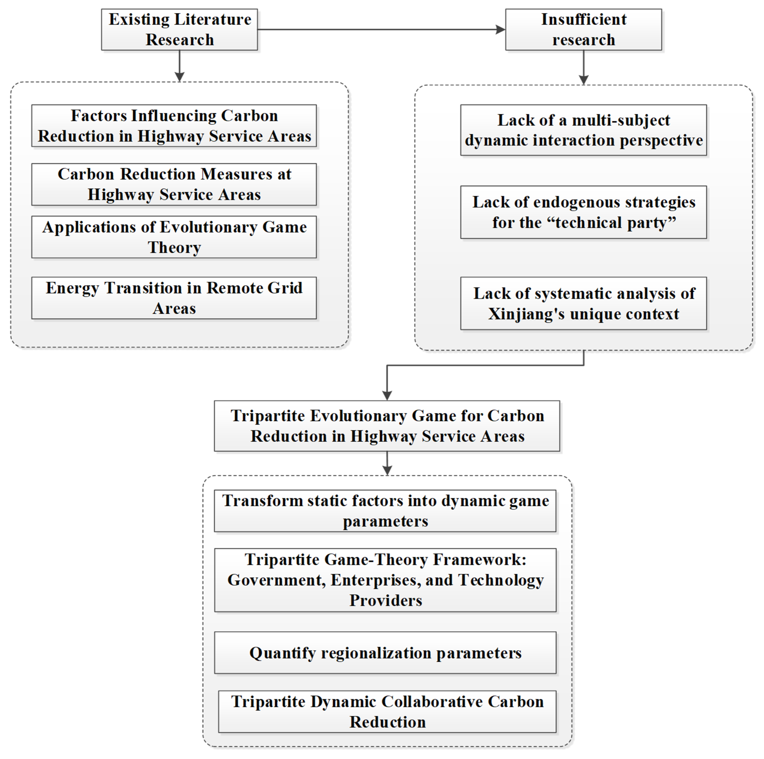
Figure 1. Research Gap in Carbon Reduction at Highway Service Areas and Tripartite Game Theory Framework Correlation Diagram.
Sustainability 17 10145 g001
Figure 2. Technology Roadmap.
Sustainability 17 10145 g002
Figure 3. Tripartite Evolutionary Game Tree Model Diagram.
Sustainability 17 10145 g003
Figure 4. Phase Diagram of the Evolution of Government Carbon Reduction Strategies for Xinjiang Highway Service Areas.
Sustainability 17 10145 g004
Figure 5. Phase Diagram of Carbon Reduction Strategy Evolution of Operating Enterprises for Xinjiang Highway Service Areas.
Sustainability 17 10145 g005
Figure 6. Phase Diagram of Carbon Reduction Strategy Evolution of Technical Support Providers for Xinjiang Highway Service Areas.
Sustainability 17 10145 g006
Figure 7. Tripartite Evolution Pathway Diagram. (a) Front View of the Three-Way Evolution Path Diagram. (b) Side View of the Three-Dimensional Evolution Pathway Diagram.
Sustainability 17 10145 g007
Figure 8. Effect of Initial Values x, y, z on Results (2D and 3D). (a) The Effect of Initial Values x, y, z on Results in a Two-Dimensional Graph. (b) The Effect of Initial Values x, y, z on Results: Three-Dimensional Diagram.
Sustainability 17 10145 g008
Figure 9. Effect of Initial Value x on y.
Sustainability 17 10145 g009
Figure 10. Effect of Initial Value x on z.
Sustainability 17 10145 g010
Figure 11. Effect of Initial Value y on z.
Sustainability 17 10145 g011
Figure 12. Impact of Increased Costs from Government Regulation on Evolutionary Outcomes. (a) Three-Dimensional Diagram of the Effect of Parameter Cg1 Variation on Results. (b) Two-Dimensional Diagram of the Effect of Parameter Cg1 Variation on Results.
Sustainability 17 10145 g012
Figure 13. Impact of Weak Regulatory Environment on Environmental Governance Costs and Evolutionary Outcomes. (a) Three-Dimensional Diagram of the Effect of Parameter Cg2 Variation on Results. (b) Two-Dimensional Diagram of the Effect of Parameter Cg2 Variation on Results.
Sustainability 17 10145 g013
Figure 14. Impact of Additional Subsidies for Corporate “Voluntary Carbon Reduction” Under Government-Mandated Regulation on Evolutionary Outcomes. (a) Three-Dimensional Diagram of the Effect of Parameter S Variation on Results. (b) Two-Dimensional Diagram of the Effect of Parameter S Variation on Results.
Sustainability 17 10145 g014
Figure 15. Impact of Government Subsidies for Active Cooperation by Technology Supporters on Evolutionary Outcomes Under Strong Regulation. (a) Three-Dimensional Diagram of the Effect of Parameter M Variation on Results. (b) Two-Dimensional Diagram of the Effect of Parameter M Variation on Results.
Sustainability 17 10145 g015
Figure 16. Impact of Positive Social Benefits from Strong Government Regulation on Evolutionary Outcomes. (a) Three-Dimensional Diagram of the Effect of Parameter Bg Variation on Results. (b) Two-Dimensional Diagram of the Effect of Parameter Bg Variation on Results.
Sustainability 17 10145 g016
Figure 17. Impact of Government-Imposed Fines for “Passive Carbon Reduction” on Evolutionary Outcomes. (a) Three-Dimensional Diagram of the Effect of Parameter F Variation on Results. (b) Two-Dimensional Diagram of the Effect of Parameter F Variation on Results.
Sustainability 17 10145 g017
Figure 18. Impact of Investment Costs in Equipment and Technology for Corporate “Proactive Carbon Reduction” on Evolutionary Outcomes. (a) Three-Dimensional Diagram of the Effect of Parameter Ce1 Variation on Results. (b) Two-Dimensional Diagram of the Effect of Parameter Ce1 Variation on Results.
Sustainability 17 10145 g018
Figure 19. Impact of the Cost of “Passive Carbon Reduction” on Evolutionary Outcomes. (a) Three-Dimensional Diagram of the Effect of Parameter Ce2 Variation on Results. (b) Two-Dimensional Diagram of the Effect of Parameter Ce2 Variation on Results.
Sustainability 17 10145 g019
Figure 20. Impact of Follow-Up Maintenance Costs for Corporate “Proactive Carbon Reduction” on Evolutionary Outcomes. (a) Three-Dimensional Diagram of the Effect of Parameter Ce3 Variation on Results. (b) Two-Dimensional Diagram of the Effect of Parameter Ce3 Variation on Results.
Sustainability 17 10145 g020
Figure 21. Impact of Economic Savings and Benefits from Corporate “Proactive Carbon Reduction” on Evolutionary Outcomes. (a) Three-Dimensional Diagram of the Effect of Parameter Re Variation on Results. (b) Two-Dimensional Diagram of the Effect of Parameter Re Variation on Results.
Sustainability 17 10145 g021
Figure 22. The Impact of the Elasticity Coefficient of Corporate Voluntary Carbon Reduction Efforts on Evolutionary Outcomes. (a) Three-Dimensional Diagram of the Effect of Parameter k Variation on Results. (b) Two-Dimensional Diagram of the Effect of Parameter k Variation on Results.
Sustainability 17 10145 g022
Figure 23. Impact of Potential Revenue from Brand Premium and Other Benefits of Corporate “Proactive Carbon Reduction” on Evolutionary Outcomes. (a) Three-Dimensional Diagram of the Effect of Parameter V Variation on Results. (b) Two-Dimensional Diagram of the Effect of Parameter V Variation on Results.
Sustainability 17 10145 g023
Figure 24. Impact of the Enhancement Coefficient for Technological Support Providers’ Benefits from Corporate “Proactive Carbon Reduction” on Evolutionary Outcomes. (a) Three-Dimensional Diagram of the Effect of Parameter β Variation on Results. (b) Two-Dimensional Diagram of the Effect of Parameter β Variation on Results.
Sustainability 17 10145 g024
Figure 25. Impact of Additional Costs from Active Cooperation by Technical Support Providers on Evolutionary Outcomes. (a) Three-Dimensional Diagram of the Effect of Parameter Ct1 Variation on Results. (b) Two-Dimensional Diagram of the Effect of Parameter Ct1 Variation on Results.
Sustainability 17 10145 g025
Figure 26. Impact of Losses from Passive Cooperation by Technical Support Providers on Evolutionary Outcomes. (a) Three-Dimensional Diagram of the Effect of Parameter Ct2 Variation on Results. (b) Two-Dimensional Diagram of the Effect of Parameter Ct2 Variation on Results.
Sustainability 17 10145 g026
Figure 27. Impact of Incremental Benchmark Gains from “Active Cooperation” by Technical Support Providers on Evolutionary Outcomes. (a) Three-Dimensional Diagram of the Effect of Parameter Rt Variation on Results. (b) Two-Dimensional Diagram of the Effect of Parameter Rt Variation on Results.
Sustainability 17 10145 g027
Figure 28. Impact of the “Active Cooperation” Factor of Technical Support Providers on Evolutionary Outcomes Regarding Cost Reduction Coefficients for Enterprises. (a) Three-Dimensional Diagram of the Effect of Parameter α Variation on Results. (b) Two-Dimensional Diagram of the Effect of Parameter α Variation on Results.
Sustainability 17 10145 g028
Table 1. Comparison Table of Three-Party and Two-Party Games.
Comparison DimensionTripartite Model (Government-Enterprise-Technology Provider)Government-Enterprise Dual ModelThe Unique Value of the Tripartite Model
Main ComponentsThree endogenous entities, with the technology provider possessing independent decision-making authorityTwo endogenous entities, with technology as an exogenous variableAddressing the core practical challenge of “technical compatibility difficulties”
Interactive MechanismTwo-way feedback (government → technology → enterprise → technology)Unidirectional Incentive (Government Subsidies → Corporate Carbon Reduction)Establish a positive feedback loop of “technology iteration—cost reduction” to avoid the linear dependency inherent in the two-party model.
Characteristics of Evolutionary OutcomesConverges to ESS (1,1,1)Single stable point: Converging toward “strong regulation—proactive carbon reduction”Identify the cost threshold of recognition technology to provide precise basis for policy formulation
Table 2. List of Parameters and Definitions.
Model StakeholderParameterParameter Definition
GovernmentCg1Increased costs resulting from stringent government regulation
Cg2The environmental governance costs incurred by the government’s adoption of weak regulation
Cg3The government’s fixed costs for regulating carbon reduction at highway service areas
SAdditional subsidy amount for enterprises’ voluntary carbon reduction efforts under the government’s stringent regulatory environment
MAdditional policy support subsidies provided by the government’s stringent regulatory environment to encourage proactive carbon reduction development cooperation among technology providers
BgThe positive social benefits resulting from the government’s implementation of stringent regulatory oversight.
FGovernment-imposed fines on companies for “passive carbon reduction” under stringent regulation
Service Area OperatorCe1The investment costs for equipment and technology associated with enterprises’ proactive carbon reduction efforts
Ce2The Cost of “Passive Carbon Reduction” for Enterprises
Ce3Follow-up maintenance costs for enterprises’ proactive carbon reduction efforts
Ce4Baseline Costs for Service Area Carbon Reduction Management in Enterprises
ReEconomic Savings and Benefits from Corporate “Proactive Carbon Reduction”
kRevenue elasticity coefficient (k > 0) indicates the amplification effect of corporate proactive carbon reduction efforts on revenue.
VPotential revenue generated from brand premiums resulting from enterprises’ proactive carbon reduction efforts
LLosses incurred by enterprises due to inadequate adaptation of carbon reduction technologies or impacts from extreme environmental conditions
βThe multiplier effect of corporate “proactive carbon reduction” on the revenue of technology providers
Technical Support ProviderCt1Additional costs incurred from the technical support provider actively cooperating
Ct2Opportunity cost losses, reputational damage, and market risk costs resulting from the passive cooperation of the technical support provider.
Ct3The benchmark cost that the technical support provider charges to provide technical services for carbon reduction in the service area.
RtIncremental benchmark gains resulting from the technical support provider’s “proactive cooperation”
QThe benchmark revenue for the carbon reduction technology service area provided by the technical support provider at the high-speed service area.
αThe coefficient of cost reduction for enterprises through “active cooperation” with the technical support providers
Table 3. Tripartite Evolutionary Game Payoff Matrix.
Government ChoiceSelection of Service Area Operating CompaniesSelection of
Technical Support Provider
Government RevenueRevenue of Service Area Operating EnterprisesRevenue for the Technical
Support Provider
Strict regulation (x)Proactive carbon reduction (y)Active cooperation (z)Bg-Cg3-Cg1-S-MkRe + V + S-Ce4 − (1 − α)(Ce1 + Ce3)-LQ + Rtβ + M-Ct3-Ct1
Passive cooperation (1 − z)Bg-Cg3-Cg1-SkRe + V+S-Ce4-(Ce1 + Ce3)-LQ-Ct3-Ct2
Passive carbon reduction
(1 − y)
Active cooperation (z)Bg + F-Cg3-Cg1-M−Ce4-Ce2-F-LQ + Rt + M-Ct3-Ct1
Passive cooperation (1 − z)Bg + F-Cg3-Cg1−Ce4-Ce2-F-LQ-Ct3-Ct2
Weak regulation (1 − x)Proactive carbon reduction (y)Active cooperation (z)−Cg3-Cg2kRe + V-Ce4-(1 − α)(Ce1 + Ce3)-LQ + Rtβ + M-Ct3-Ct1
Passive cooperation (1 − z)−Cg3-Cg2kRe + V-Ce4-(Ce1 + Ce3)-LQ-Ct3-Ct2
Passive carbon reduction
(1 − y)
Active cooperation (z)−Cg3-Cg2−Ce4-Ce2-LQ + Rt-Ct3-Ct1
Passive cooperation (1 − z)−Cg3-Cg2−Ce4-Ce2-LQ-Ct3-Ct2
Table 4. Eigenvalues and Stability Conditions.
Equilibrium PointEigenvalue 1Eigenvalue 2Eigenvalue 3Stable Condition
Expression+/−Expression+/−Expression+/−
E1 (0,0,0)Bg-Cg1 + Cg2 + FUncertainCe2-Ce1-Ce3 + kRe + VUncertainCt1-Ct2-RtUncertainWhen Bg + Cg2 + F < Cg1 and Ce2 + kRe + V < Ce1 + Ce3 and Ct1 < Ct2 + Rt, ESS
E2 (0,1,0)Bg-Cg1 + Cg2-SUncertainCe1-Ce2 + Ce3-kRe-VUncertainCt2-Ct1 + βRtUncertainWhen Bg + Cg2 < Cg1 + S and Ce1 + Ce3 < Ce2 + Re*k +V and Ct2 + βRt < Ct1, ESS
E3 (0,0,1)Bg-Cg1 + Cg2 + F-MUncertainCe2-Ce1-Ce3 + kRe + V+α(Ce1 + Ce3)UncertainCt1-Ct2-RtUncertainWhen Bg + Cg2 + F < Cg1 + M and Ce2 + kRe + V < (1 − α)(Ce1 + Ce3) and Ct1 < Ct2 + Rt, ESS
E4 (0,1,1)Bg-Cg1 + Cg2-M-SUncertainCe1-Ce2 + Ce3-kRe-V-α(Ce1 + Ce3)UncertainCt1-Ct2-βRtUncertainWhen Bg + Cg2 < Cg1 + M+S and (1 − α)(Ce1 + Ce3) < Ce2 + kRe + V and Ct1 < Ct2 + βRt, ESS
E5 (1,0,0)Cg1-Bg-Cg2-FCe2-Ce1-Ce3 + F+kRe + S+VUncertainCt2-Ct1 + M+RtUncertainWhen Ce2 + F+kRe + S+V < Ce1 + Ce3 and Ct2 + M+Rt < Ct1, ESS
E6 (1,1,0)Cg1-Bg-Cg2 + SUncertainCe1-Ce2 + Ce3-F-kRe-S-VUncertainCt2-Ct1 + M+βRtUncertainWhen Cg1 + S < Bg + Cg2 and Ce1 + Ce3 < Ce2 + F+kRe + S+V and Ct2 + M+βRt < Ct1, ESS
E7 (1,0,1)Cg1-Bg-Cg2-F + MUncertainCe2-Ce1-Ce3 + F+kRe + S+V + α(Ce1 + Ce3)+Ct1-Ct2-M-RtUncertainInstability point or saddle point
E8 (1,1,1)Cg1-Bg-Cg2 + M+SUncertainCe1-Ce2 + Ce3-F-kRe-S-V-α(Ce1 + Ce3)Ct1-Ct2-M-βRtUncertainWhen Cg1 + M+S < Bg + Cg2 and Ct1 < Ct2 + M+βRt, ESS
Table 5. Simulation Parameter Assignments.
Cg1Cg2SMBgFCe1Ce2Ce3RekVCt1Ct2Rtαβ
583310241111110530.52
Disclaimer/Publisher’s Note: The statements, opinions and data contained in all publications are solely those of the individual author(s) and contributor(s) and not of MDPI and/or the editor(s). MDPI and/or the editor(s) disclaim responsibility for any injury to people or property resulting from any ideas, methods, instructions or products referred to in the content.